The Composite Method: A Novel, Continuum-Based Approach to Estimating Age from the Female Pubic Symphysis with Particular Relevance to Mature Adults

Abstract

While a myriad of effective techniques exist to aid in symphyseal age estimation for those 40 years and younger, few offer similar levels of efficacy for those beyond that threshold. Through the application of a novel technique, this study sought to determine whether a closer inspection of degenerative change may help to improve precision in age estimation for post-epiphyseal adults. Results show that the combination of five distinct areas of interest, plus a correction for density, accurately estimated age 87.75% of the time (averaged amongst four observers [spread: 72–100%]) for a subset of 50 living British females. An adjusted R² value of 0.85, an RSME value of 5.62 years, and a PCC value of 0.92 also confirmed the trialed technique to be a good predictor of age for the entirety of the larger female sample (n = 533). Low inaccuracy (3.86 years) and Bias (0.69 years) further indicate that a continuum-based approach, without pre-set phases or ranges, such as was utilized by this research holds the potential to be at least as effective as the currently available methodologies but with the added advantage of allowing for increased variation at the individual level. Age estimation by linear regression, or by simple addition, yielded estimation envelopes (intervals) of 22–23 and 24 years, respectively, which remain narrow enough to be forensically useful while still wide enough to maximize accuracy in mature adults.

1. Introduction

Age estimation from the adult skeleton is often described as a balancing act between accuracy and precision—“when one goes up, the other goes down” [1] (p. 230). Leaning too heavily towards accuracy (whether an estimated age falls within an expected range) often results in prediction envelopes that are unhelpfully broad, while leaning too heavily towards precision (the distance between estimated and actual age) risks loss of applicability. This is especially true for mature adults for whom senescence, a highly individual process influenced by both biology and environment [2,3,4,5,6,7], has replaced development as the primary agent of osteological change [8,9,10,11,12,13].

This is because, while the emergence of dentition and the epiphyseal fusions of youth exhibit clearly defined transitions, skeletal modification during the second half of life presents much more subtly and becomes increasingly fluid in its timing with advancing age. This ambiguity has led to an ongoing debate as to whether post-fusion individuals may be meaningfully aged at all, with recent scholarship [14,15,16,17,18,19,20,21,22,23,24,25,26,27,28,29,30,31,32] failing to supplant more cautious catch-all categories, such as “65+”, “old adult”, or “elderly”. However, with one in six people worldwide (including one in four in Europe and North America) projected to reach 65 years or older by 2050, and the number of those aged 80 years or more expected to triple [33,34], relying on large, multi-decade ranges for older individuals for forensic casework may soon prove to be unsustainable.

This research sought to investigate whether an underlying uniformity of degenerative change—generally thought to be more obstructive than instructive—may, in itself, be as effectively diagnostic in the latter half of life as dental eruption and epiphyseal union are to the first. For this, the pubic symphysis was chosen, due to its sustained popularity amongst practitioners [11,35], its extensive literature base and diversity of analytical approaches [36,37,38,39,40,41,42,43,44,45,46,47,48,49,50,51,52,53,54,55,56,57,58,59,60,61,62,63,64,65,66,67,68,69,70,71,72,73], and its longevity as an articulation exhibiting continuous activity throughout the entirety of adult life. The female symphysis was then prioritized as females have been historically considered to be more irregular in their variation, leading to greater estimation uncertainty at any age [37,38,40,54,55,56,60,74,75,76,77,78,79,80].

Through the development of a novel continuum-based approach, the following three objectives were pursued: (1) the utilization of a large multi-faceted dataset composed of face-to-face interviews, questionnaires, and medical imaging of currently living volunteers, (2) the creation of an age-estimation technique focusing specifically on senescent change at the pubic symphysis, and (3) a review of the trialed technique via statistical analysis to assess its efficacy for age estimation in mature adults.

2. Materials and Methods

The parent sample for this research consisted of 1238 living individuals undergoing routine clinical scanning over the seven-month period between 1 September 2014 and 31 March 2015 at the National Health Service (NHS) Oxford University Hospital System’s (OUHS) Churchill Hospital in Headington, UK. All patients receiving a CT scan in which the pubic symphysis would be captured were invited to participate. The volunteers were asked to complete either a four- (males) or six- (females) page questionnaire detailing their demographic, environmental, lifestyle, and parity information. Each participant was then interviewed “face-to-face” by the author, both to verify the answers given and to follow up where necessary, prior to the individual proceeding to his or her scan. All scans were performed by OUHS Churchill Hospital staff radiographers, each of whom was professionally trained and fully qualified to produce scans at a clinical level of competency.

This study was approved by the UK National Research Ethics Service (NRES) (NRES ID: 119232, Research Ethics Committee [South Central—Hampshire A] ref: 14/SC/0061), Oxford University Hospitals (OUH) National Health Service (NHS) Trust Management (HH/BS/DF/8851), and Oxford University’s Central University Research Ethics Committee (CUREC). Written informed consent was obtained from each participant.

2.1. Sample

Of the 1238 participants, 653 were male and 585 were female. A total of 82 individuals were excluded due to a scan defect, obscuring artifact, or duplication. Of these exclusions, 52 were female, resulting in a final female n of 533. Of those 533, 512 (96%) individuals identified as White, while 21 (4%) individuals identified as either South Asian, East Asian, Black (African or Caribbean), Arab, multiple ethnicity, or other ethnicity (

Table 1. Descriptive statistics: Ancestry by age group (females, n = 533).

Age Group	n =	White	Asian—South	Asian—East	Black (African or Caribbean)	Arab	Multiple Ethnicity *	Other Ethnicity †
18–19	4	3					1
20–29	9	8					1
30–39	29	27	1		1
40–49	42	40				1
50–59	117	109	1		4		1	1
60–69	137	130	1		1		3	2
70–79	149	147			1		1
80–89	42	42
90–99	4	4
Total:	533	512	3	0	7	1	7	3

* Of the “multiple ethnicities” reported, two individuals identified as White/South Asian (Indian), one individual identified as White/East Asian (Indian and Malay), two individuals identified as White/Black (African or Caribbean), one individual identified as White/Black (African or Caribbean) (St. Helena Island), and one individual identified as White/Black (African or Caribbean) (North African, Tunisia). ^† Of the “other” ethnicities reported, two individuals identified as Ashkenazi Jew and one individual identified as Brazilian.

). While imperfect, this terminology was directed by the overseeing research ethics committee in order to mirror existing UK government census categories.

Though constituting a comparatively small percentage of the overall sample, the non-White participants did not present as outliers when actual age and estimated age were compared (n = 21; t = −0.25817, df = 39.987, p-value = 0.7976; RSME: 3.29) and were therefore not excluded from the final analysis. As the subjects were fully anonymized and no chance existed of identification through demographic information (even in small number), this served to both strengthen the dataset and to preserve a more accurate representation of the Oxford population.

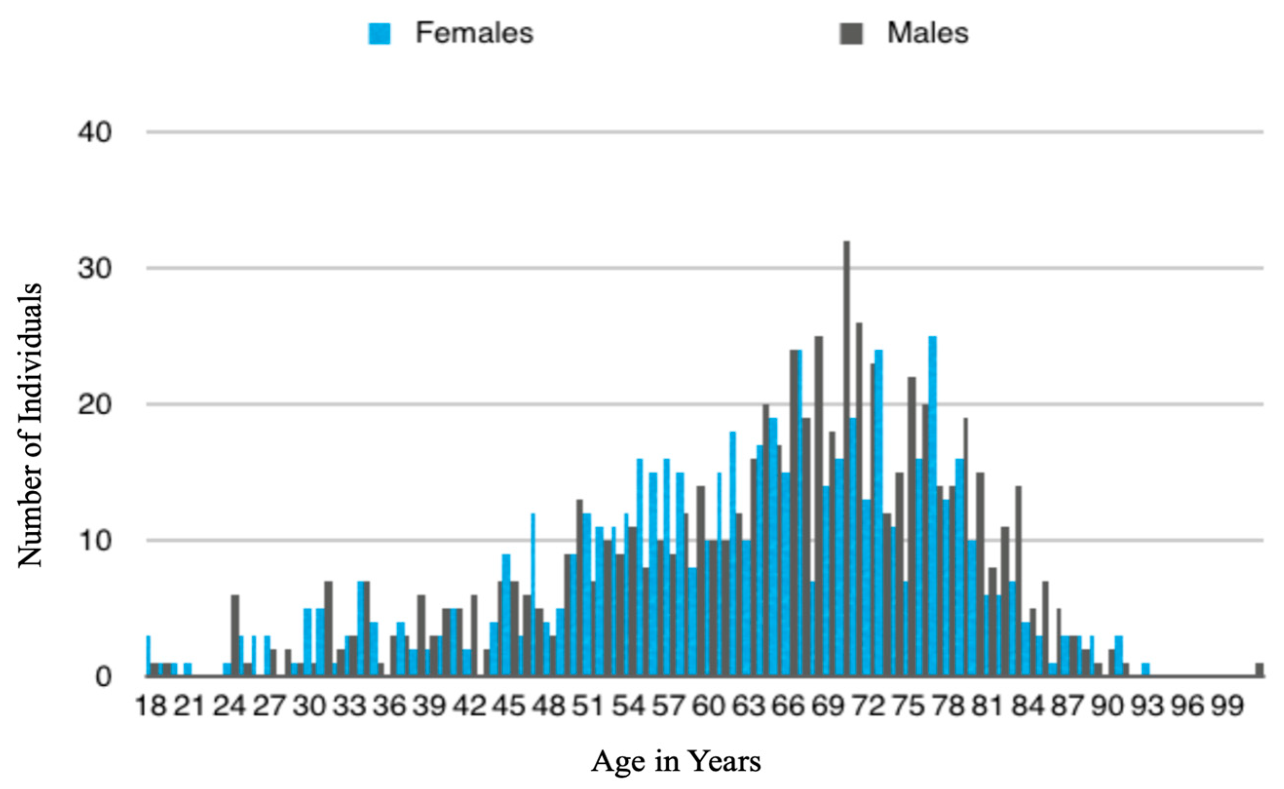
The average age of the females in this sample was 62.65 years, with the majority of participants falling between the ages of 50 and 85 years (Figure 1).

The most commonly reported height was 160–170 cm (5′2”–5′6”). The average weight was 70.3 kg (155 pounds), with 453 (85%) participants reporting that their weight had not fluctuated by more than 10 kg (22 pounds) during the 5 years prior to their scan. A total of 53 (10%) females in this sample reported themselves to be active, 282 (53%) reported themselves to be moderately active, 192 (36%) reported themselves to be lightly active, and 6 (1%) reported themselves to be inactive or immobile. Of the active and moderately active, 53 (10%) participants reported regularly engaging in activities that involved repetitive core twisting and/or pelvic stabilization motions. A total of 309 (58%) participants reported themselves to have a healthy or better-than-average diet, 208 (39%) reported an average diet, and 16 (3%) reported a poor or insufficient diet. A total of 400 (75%) females in this study reported themselves to be non-smokers, while 53 (10%) reported themselves to be current tobacco smokers (most commonly 20 cigarettes, or approximately “1 pack”, per day). A total of 80 (15%) individuals reported themselves to be former smokers who had quit prior to their scan. A total of 341 (64%) females in this study reported themselves to be current alcohol consumers (most commonly 10 units or fewer per week), while 16 (3%) reported themselves to be former consumers who had quit consumption prior to scanning. A total of 3 (0.05%) individuals reported a previous diagnosis of osteitis pubis (treated successfully prior to scanning), 16 (3%) reported a history of chronic or persistent urinary tract infections, 112 (21%) reported diagnoses of osteopenia or osteoporosis, and 288 (54%) reported chronic joint pain and/or arthritis.

The participants were initially separated by parity; however, as the distance between the estimated age for the parous (n = 453; t = −0.5063, df = 883.38, p = 0.613) and nulliparous (n = 80; t = −0.57157, df = 157.91, p = 0.568) groups and actual age was too small to be significant, the two groups were pooled into one larger, more robust dataset. Ordering department was also investigated but was found to have no impact on age estimation in this study (

Table 2. T-test analyses comparing estimated mean age versus actual age by ordering department.

	Entire Sample (n = 1156)				Females Only (n = 533)
		t	df	p		t	df	p
Oncology	n = 380	−1.0313	834.47	0.3027	n = 183	−0.4749	357.16	0.6352
Urology	n = 255	−0.4685	496.13	0.6396	n = 101	−0.4317	199.2	0.6664
Gastroenterology	n = 111	−0.3096	214.79	0.7571	n = 49	0.0954	92.555	0.9242
Pre-Op	n = 104	−0.4868	200.81	0.6269	n = 53	−0.4847	103.28	0.6289
GP/Private Care	n = 90	−1.6255	173.73	0.1059	n = 38	−0.6999	73.159	0.4862
Haematology	n = 44	−0.5710	83.942	0.5695	n = 25	0.0722	46.811	0.9428
Cardio/Pulmonary	n = 11	−0.0570	19.095	0.9551	n = 7	0.0955	11.781	0.9255
Unspecified	n = 127	−0.3340	239.21	0.7387	n = 62	0.1316	121.52	0.8956
Miscellaneous	n = 34	—	—	—	n = 15	—	—	—

).

2.2. Instrumentation

Each of the scans utilized as part of this study were performed with one of two 64-Slice Light Speed Multi-Detector Volumetric Computed Tomography (VCT) machines, manufactured by General Electric Healthcare (program software: 12HW14.6_SP-1-1.V40_H64_G_GTL), located within the OUHS Churchill Hospital radiology department. Each possessed a helical acquisition with a pitch of 0.098, a tube rotation speed of 0.5 s, and a tube output of 120 kVp (peak kilovoltage). The slice thickness for each scan was between 0.6 mm and 0.8 mm. To ensure image accuracy, both machines were subject to daily, weekly, and yearly quality control checks, as legally required by the Ionizing Radiations Regulations of 1999 (IRR99 No. 3232) and the Ionizing Radiation (Medical Exposures) Regulations of 2000 (IRMER No. 1959).

2.3. Rendering and Acquisition

Once scanned, individual DICOM data from each participant were retrieved from the OUHS picture archiving and communication system (PACS) via GE Healthcare’s Advanced Workstation for Diagnostic Imaging (software version 4.5) and were 3D rendered using Volume Viewer (software version 9.5.6), allowing the images to be manually manipulated. Each anonymized scan was then analyzed by isolating the pubic symphysis from its wider context. Once isolated, the two halves were then further separated for individual study. Only the faces without obscuring pathology, defect, or artifact were analyzed. Where both symphyseal faces were available, each side was analyzed separately, followed by an averaging of their results. Where only one side was available, that side was scored unpaired. Inaccuracy and bias comparisons of right versus left versus averaged results are presented as

Table 3. Inaccuracy and bias (years): left face versus right face versus both faces averaged.

	Left			Right			Averaged
Group	n=	Inaccuracy	Bias	n=	Inaccuracy	Bias	n=	Inaccuracy	Bias
Entire Sample	1140	4.261	1.403	1140	4.427	0.396	1156	4.091	0.919
Entire Sample (50+)	964	3.474	0.195	962	3.818	−0.791	977	3.380	−0.269
Females Only	525	3.996	1.124	517	4.400	0.118	533	3.865	0.691
Females (50+)	441	3.644	0.338	436	4.105	−0.771	449	3.531	−0.126

.

3. Technique

The technique developed for this study paid homage to several extant methodologies by incorporating elements of Todd’s (36, 37) and Suchey–Brooks’ (45) visual archetype approach, McKern and Stewart’s (39, 40) component system, Hanihara and Suzuki’s (41), Snow’s (42), and Chen et al.’s (49–51) linear regressions, Berg’s (54) seventh-phase addition, and Hartnett’s (55) incorporation of density. As it represented a combination, or composite, of the prior literature, it was referred to during testing as the “combined” or “composite” method (abbreviated hereafter as “TCM”).

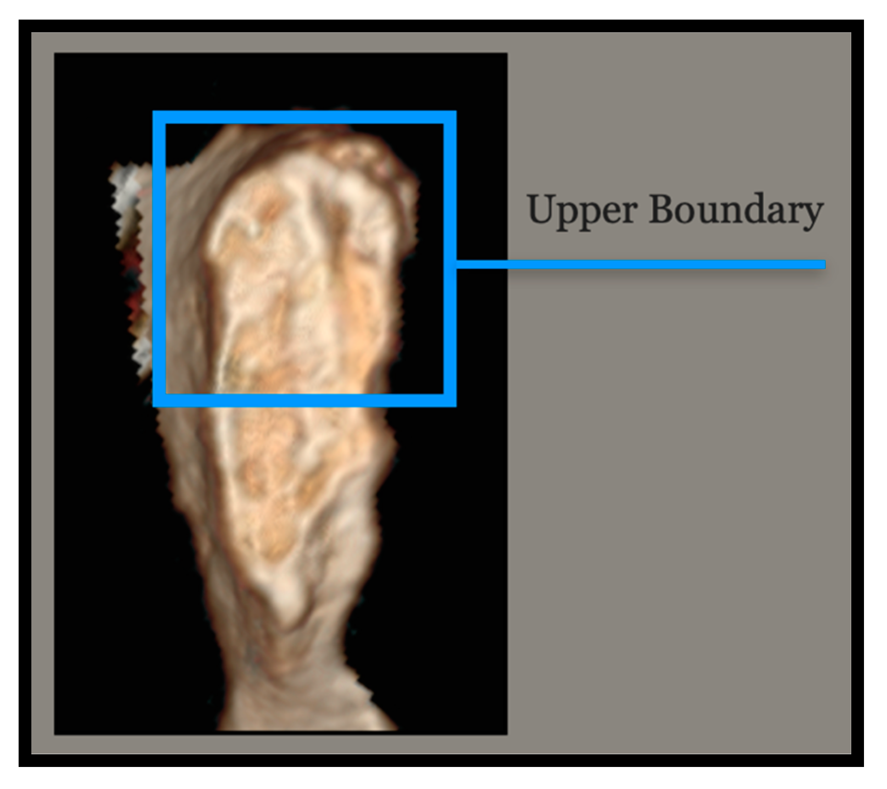
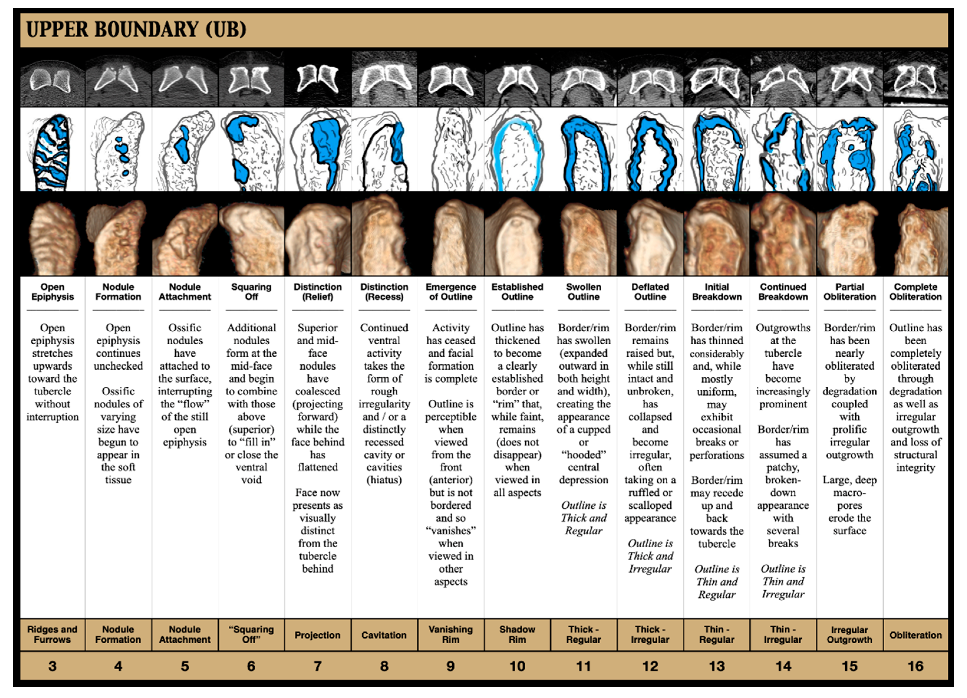
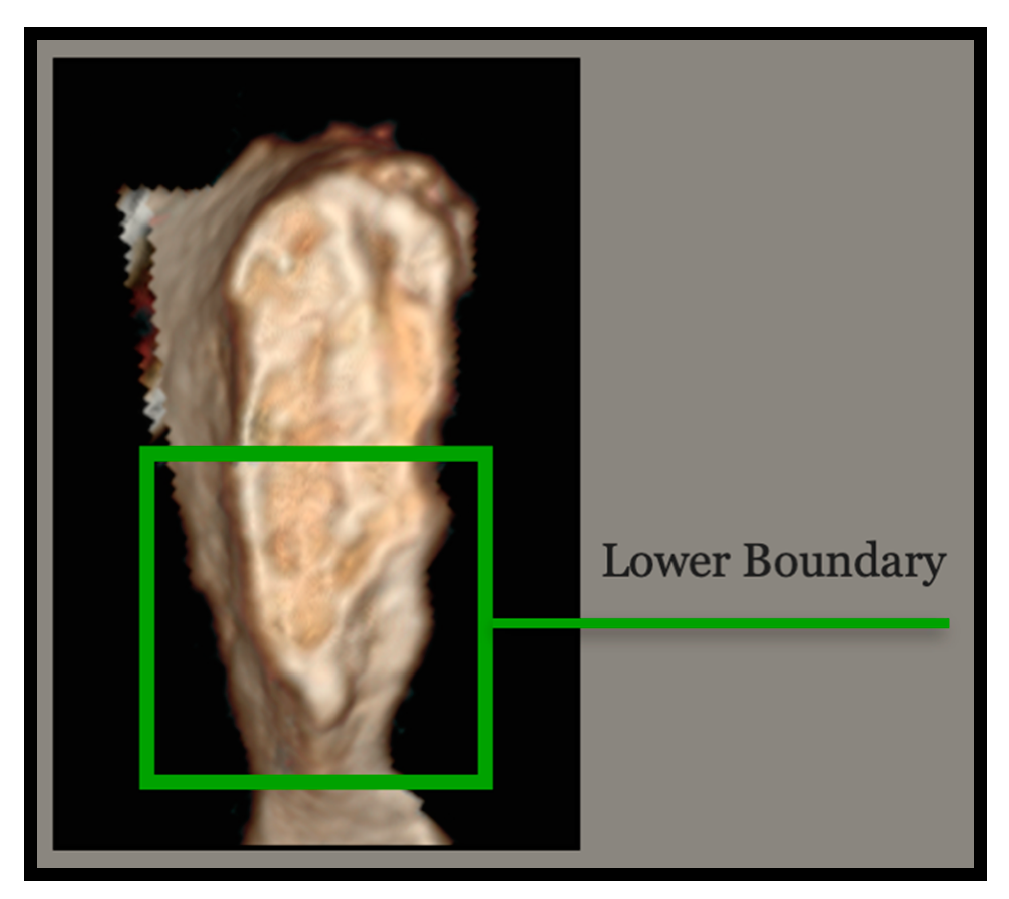
For increased specificity, the symphyseal surface was divided into five areas of interest (“AOI”), which, together, served to quickly and comprehensively document the face in its entirety. The areas that were isolated for this purpose were the upper half of the face (“Upper Boundary”), the lower half of the face (“Lower Boundary”), the overall outline of the face (“Outline”), the texture of the face (“Surface Texture”), and the raked inferior–superior view of the face (“Topography”). Backwards elimination testing showed each to be equally important to the TCM, indicating that none should be eliminated or condensed within the model. Within each of these AOI, a series of screen-captured images depicting the faces’ progression of change were presented with a line of continuous numbers—beginning with three (establishing 15 years as the lowest possible outcome) and ending with 16 (establishing 90 years as the highest possible outcome)—placed below them in order to create a set of 13 discrete columns. Each of these columns then included a stylized illustration emphasizing that “score’s” most diagnostic feature (depicted in blue) along with an explanatory title, a written description, and a key word or phrase.

Detailed descriptions of each of the five AOI are provided below and correspond with Figure 2, Figure 3, Figure 4, Figure 5, Figure 6, Figure 7, Figure 8, Figure 9, Figure 10 and Figure 11. Each AOI exists independently (meaning it is possible to have a score of 3 and a score of 16 within the same face) and may be evaluated in any order.

• Upper Boundary (UB)

The Upper Boundary (Figure 2) consists of the upper half of the face and includes the crest and tubercle behind. In evaluating the Upper Boundary, focus should be placed on activity, shape, and condition. This may include, but is not limited to, whether the epiphysis is open, whether ossific nodules are present, whether the face has flattened, or whether the face is bordered (Figure 3). Axial images were included in the guide for this AOI as they were found to be particularly diagnostic in this area.

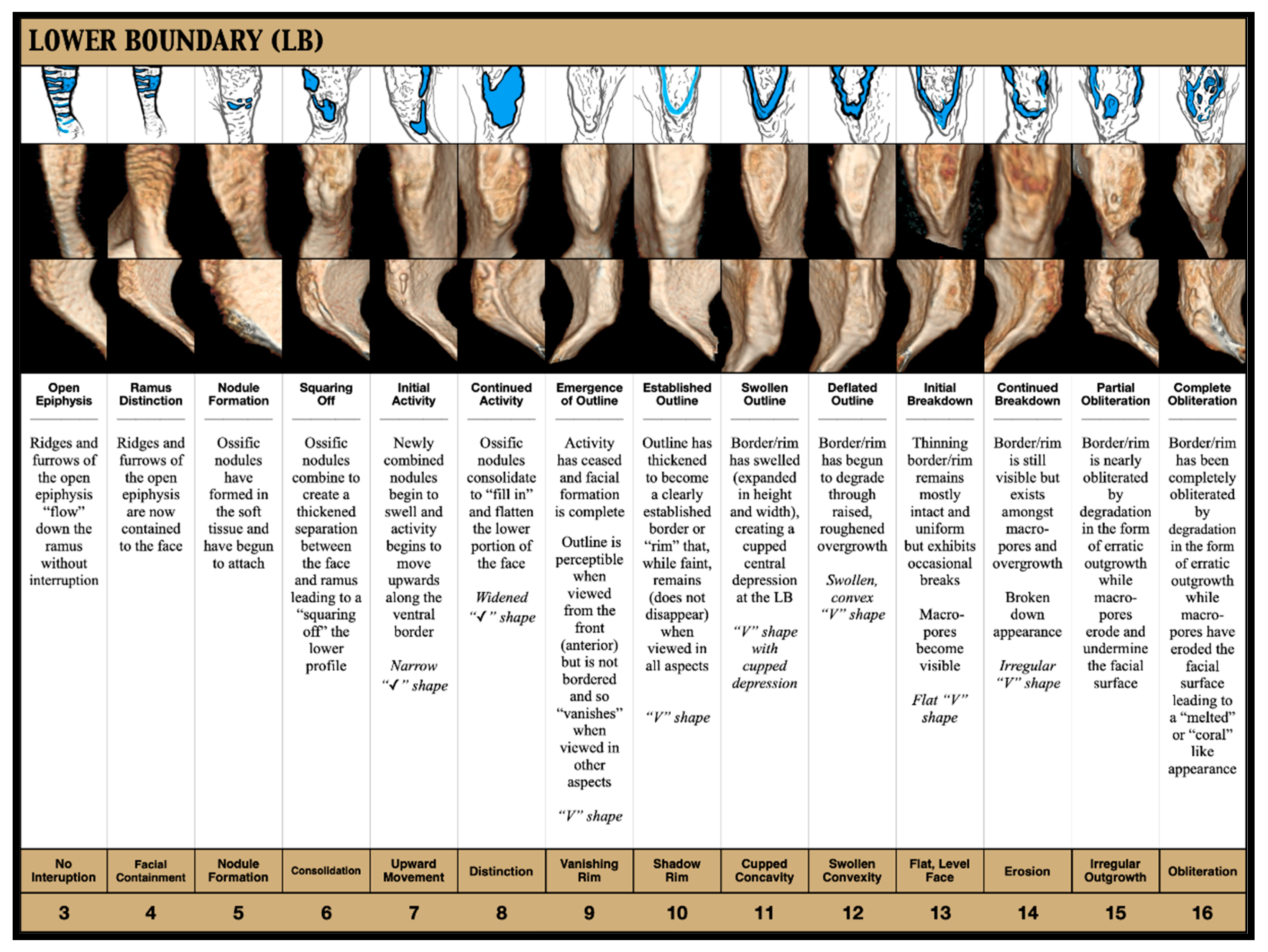
• Lower Boundary (LB)

The Lower Boundary (Figure 4) consists of the lower half of the face and includes the inferior edge and the descending ramus. In evaluating the Lower Boundary, focus should be placed on facial distinction, border shape, and condition. This may include, but is not limited to, whether the epiphysis is open, how far down the ramus activity extends, whether ossific nodules are present, whether the face has flattened, or whether the border is “✓-”, “V-”, or “U-” shaped (Figure 5).

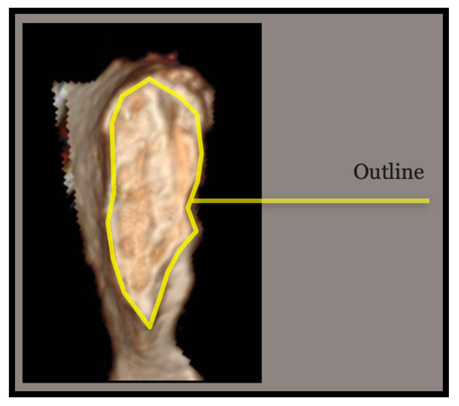
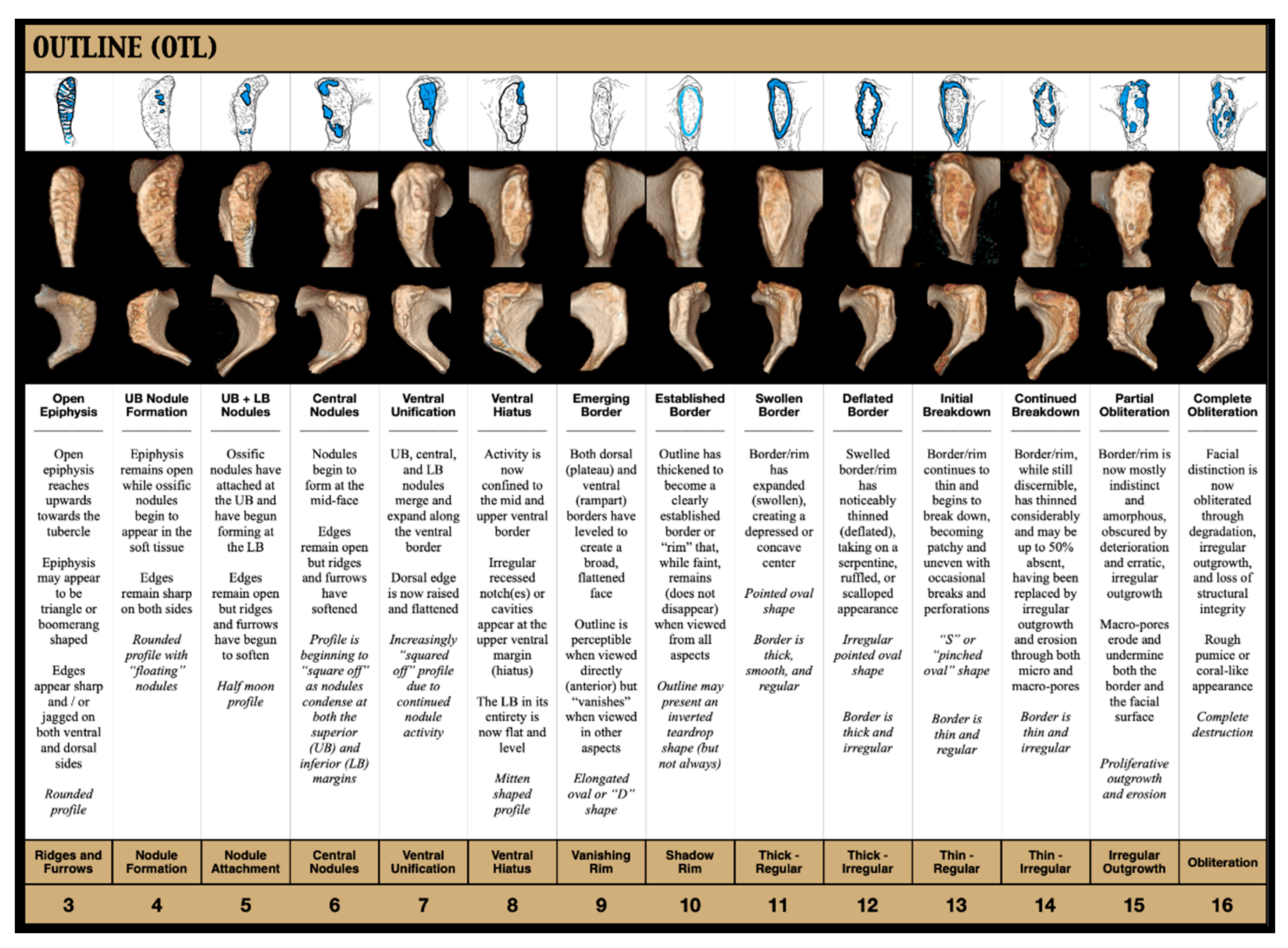
• Outline (OTL)

Unlike the Upper and Lower Boundaries, which isolate one half of the face and then the other, to assess the “Outline” (Figure 6), the practitioner must “zoom out” in order to evaluate the face as a whole. For this, only the border should be considered (Figure 7). More than any other, this AOI charts the progression of the face’s epiphyseal closure, beginning with its early build-up through the formation, the attachment, and the continued activity of the ossific nodules (numbers 3–8, approximate ages 15 to 40), its completion resulting in “squaring off” (numbers 9 and 10, approximate ages 45–50), and its eventual breakdown through erosion and deterioration (numbers 11–16, approximate ages 55 to 80+).

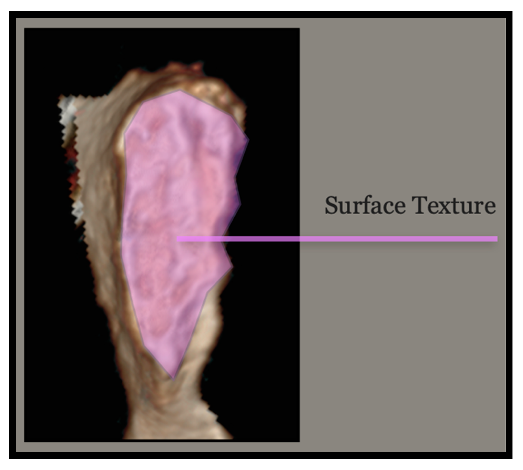
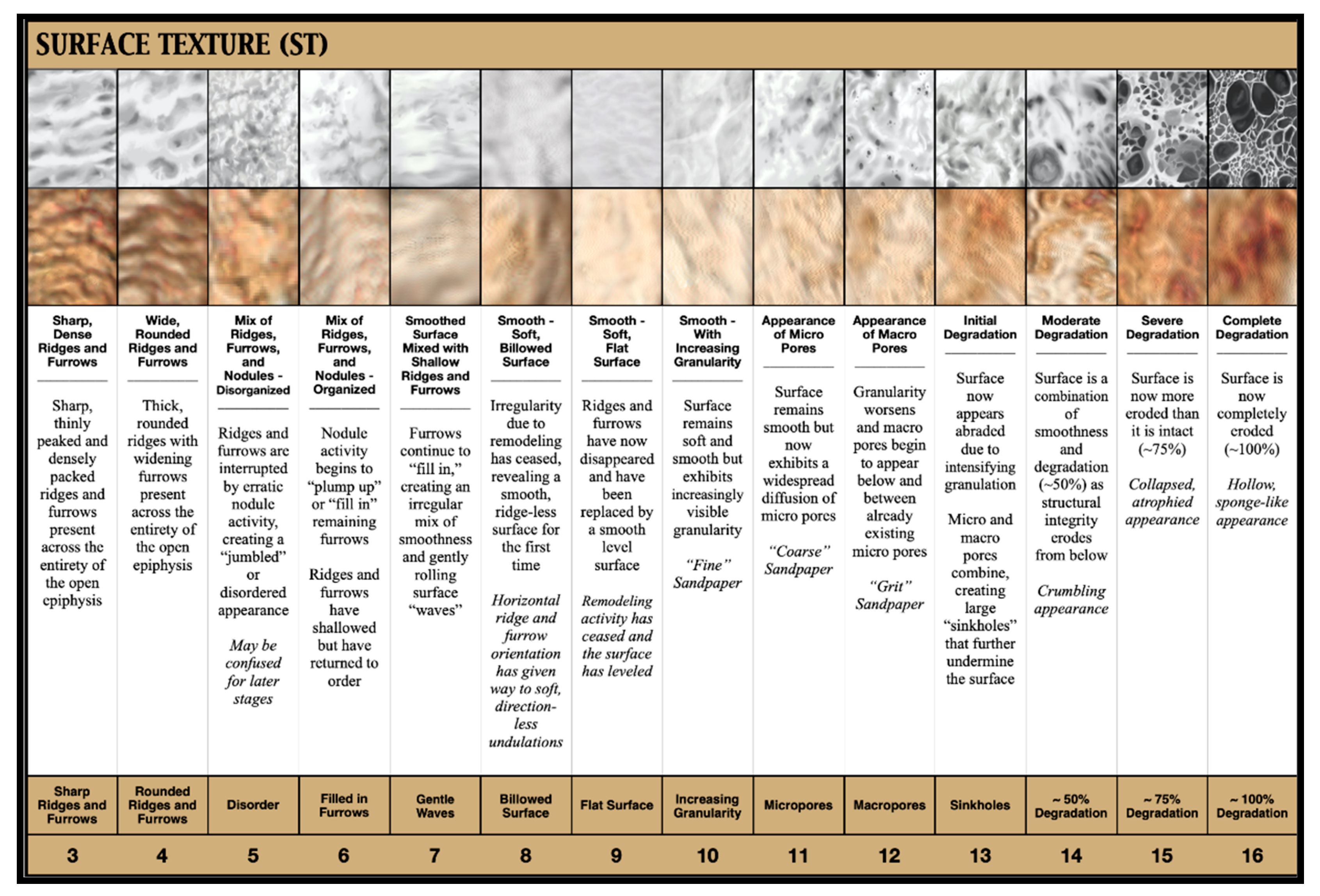
• Surface Texture (ST)

Conversely to the Outline, the “Surface Texture” (Figure 8) focuses exclusively on the texture and the structural integrity of the face itself. In early life, the pubic face is characterized by distinct “ridges and furrows” that fill in and flatten to settle into grainier sandpaper-like textures before finally eroding and “crumbling” from below in the form of first “micro-” and then “macro-” pores (Figure 9). In this study, which relied upon computed tomography and was therefore entirely image based, the tactility that is usually afforded by physical bone was replaced by algorithmically generated “shadow”. The texture was, therefore, inferred from gradations in color (light versus dark) and the ratio thereof across the face.

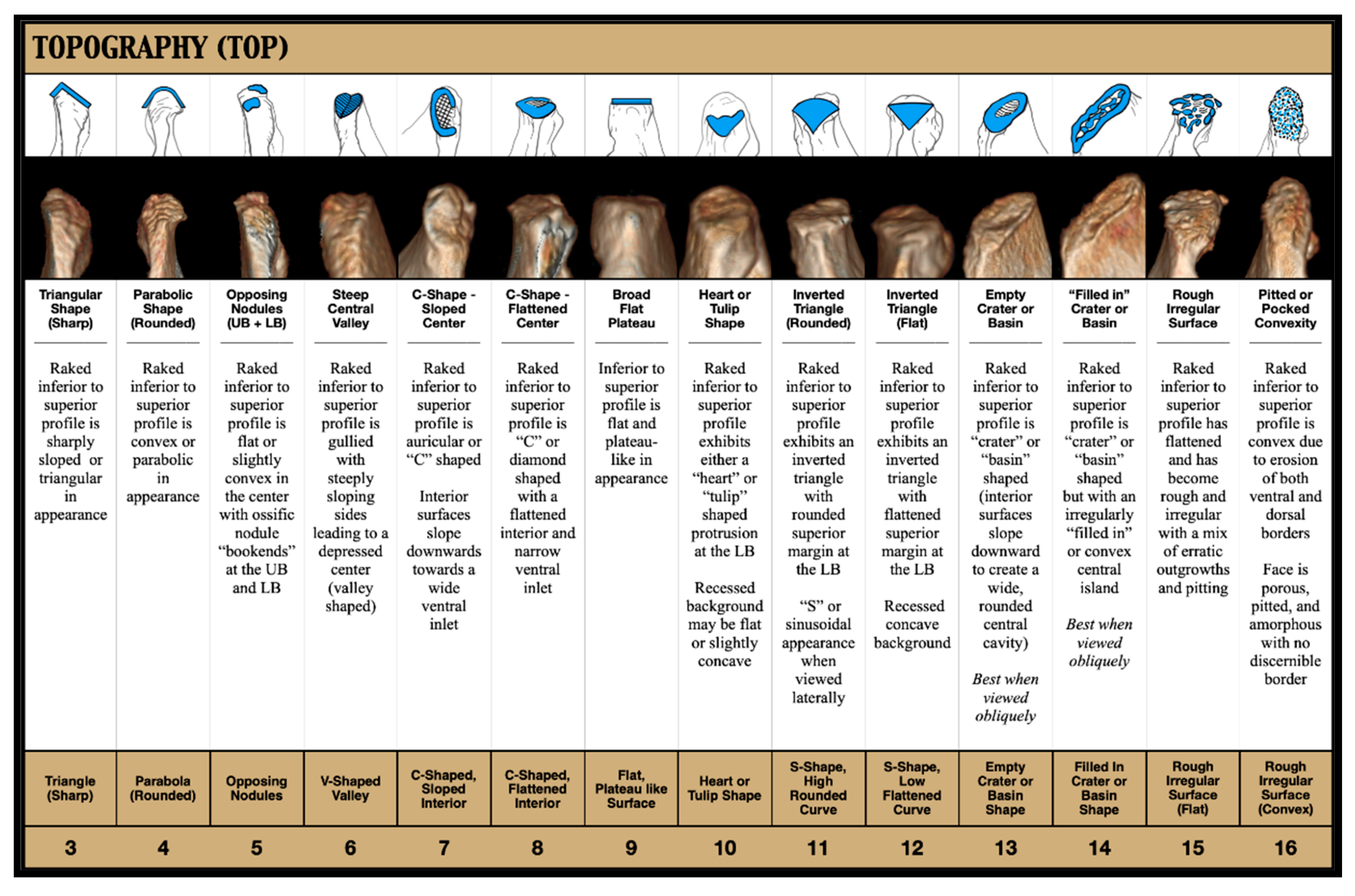
• Topography (TOP)

The final AOI was that of “Topography” (Figure 10). This AOI comes into relief when the symphyseal face is tilted back (generally between 45 and 90 degrees) and viewed from an inferior to superior “raked” angle. When it is positioned in this way, diagnostically significant shapes and contours become visible and may be assessed (Figure 11).

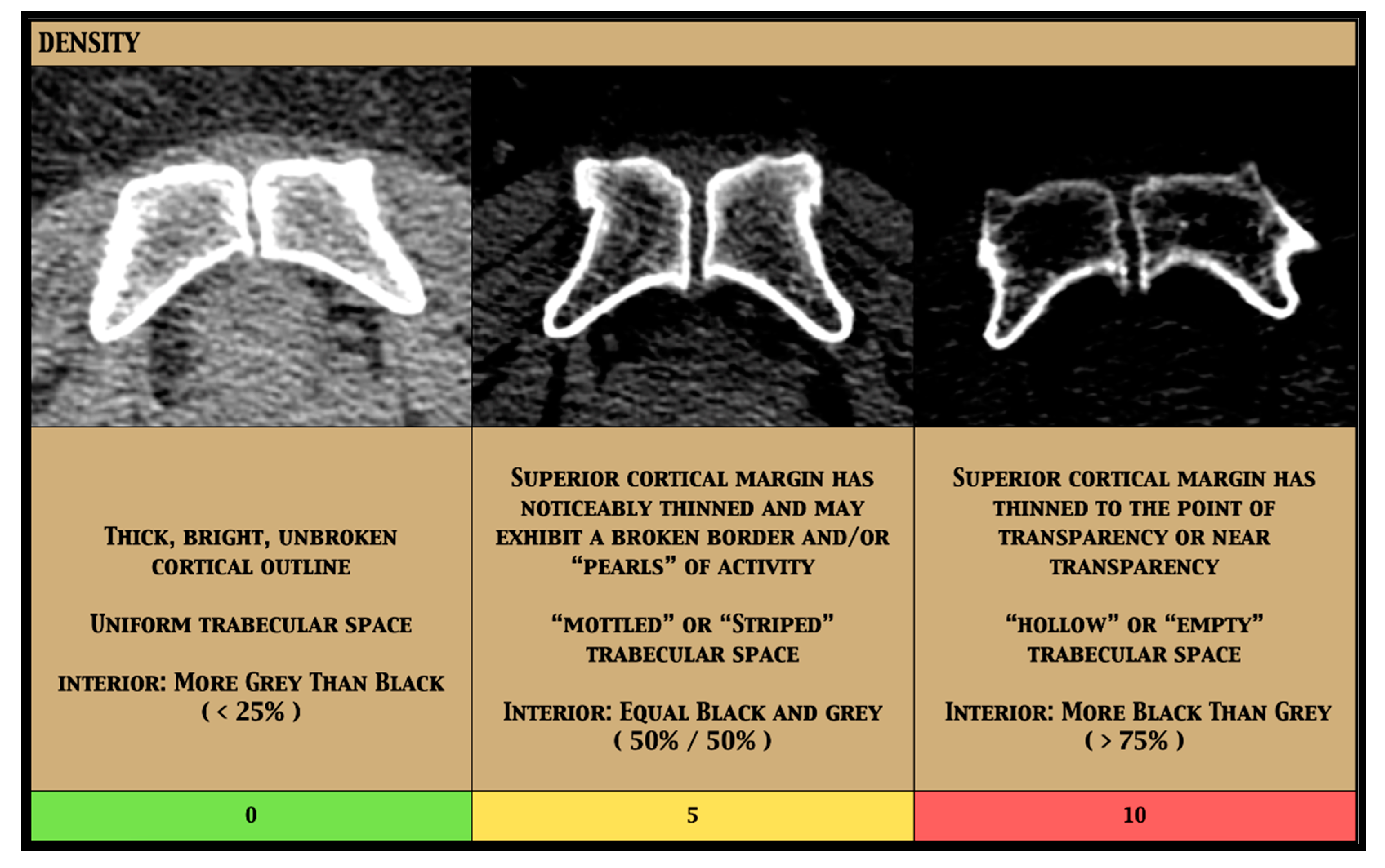
• Density Adjustment

After piloting the technique, it became clear that certain individuals were being consistently, yet predictably, under-aged and that those individuals tended to be the ones exhibiting the greatest loss of density on their axial views. Because of this, it was decided that accommodation should be incorporated as an adjustment to the overall outcome. For the females, this adjustment took the form of the following three categories: high density, which carried a weight of “0”; medium density, which carried a weight of “5”; and low density, which carried a weight of “10” (Figure 12).

3.1. Application

By employing the above AOIs, the TCM may be applied in either one of two ways—linear regression or simple addition—with equal efficacy (

Table 4. T-test and Pearson coefficient analyses comparing estimates derived by regression versus simple addition (females only, n = 533).

	Actual Age v Regression Estimates				Actual Age v Addition Estimates				Regression v Addition Estimates
	t	df	p	PCC	t	df	p	PCC	t	df	p	PCC
All Females (n = 533)	−0.0607	1057.2	0.9516	0.9245	−0.6081	1051.3	0.5433	0.9251	−0.5706	1063.0	0.5684	0.9953

).

3.1.1. Regression Approach

To investigate whether the above AOIs acted as good predictors of age, regression analysis was applied. As would be expected, the standard diagnostic checks for normality revealed that density was the only non-normally distributed variable, requiring its more categorical data to be transformed into something more continuous. In order to perform this, square roots were employed. Taking the square root of each density score, instead of the scores themselves, decreased the awkwardness of the data by narrowing the intervals between each point. This transformation of density by square rooting exhibited a normalizing effect by “bringing things into line” and allowing for easier comparison with the other AOIs. A general linear model was then fit in order to compare the independent TCM variables of “Density” (dens.sqrt), “Upper Boundary” (UB), “Lower Boundary” (LB), “Outline” (OUTL), “Surface Texture” (ST), and “Topography” (TOP) against the dependent variable of “Age”. Through step-wise regression, each of the six variables was found to be significant to the model’s ability to predict age from the os pubis (explaining 85% of the sample’s variation—Adj. R² = 0.85), meaning none could be eliminated or condensed.

For the participants in this study, the TCM was shown to predict age reasonably well (RSME = 5.62 years, R² = 0.85, PCC = 0.92) (

Table 5. TCM model accuracy.

	n=	Error	1 σ	2 σ	Inaccuracy	Bias	Adj R2	Min/Max Accuracy	MAE	RSME	PCC
Entire Sample	1156	−0.01	6.20	12.40	4.09	0.92	0.81	0.93	4.34	6.19	0.87
Females Only	533	0.2	5.66	11.32	3.86	0.69	0.85	0.94	4.00	5.62	0.92

). Mean absolute error (MAE), which does not rely upon square rooting prior to error averaging and is therefore less concerned with the magnitude of error than with the actual error (distance from the regression line), is often considered to be a more “steady” measure of model accuracy. For the females in this sample, this distance—or how close the estimated age was to actual age—translated to an average of four years.

Instructions for the regression application are as follows:

(1)

Find the pubic symphysis for the individual in question, isolate either the left or the right os pubis, and locate its articular surface, or “face”;

(2)

Looking at that face directly, locate the Upper Boundary (Figure 2);

(3)

Consult the descriptions and the images under the “Upper Boundary” heading of the TCM guide (Figure 3) and choose the column that most closely fits the individual in question;

(4)

Note the number, or the “score,” for that column and reserve it for later;

(5)

Continue steps 1–4 for each additional AOI (Figure 4, Figure 5, Figure 6, Figure 7, Figure 8, Figure 9, Figure 10 and Figure 11);

(6)

To assign the density adjustment, find the axial image in which the symphysis is at its widest (dorsoventrally), choose the “Density” column (Figure 12) that best matches the individual in question, and retain that number;

(7)

Input each number into the following equation:

−1.99 + (3.01 × sqrt{Density score}) + (0.92 × Upper Boundary score) + (0.46 × Lower Boundary score) + (1.13 × Outline score) + (1.18 × Surface Texture score) + (1.38 × Topography score) = mean age;

(8)

Add and subtract 11.32 (SD = 5.66 × 2, 95% CI) from that mean age;

(9)

The range that is produced is the estimated age for the individual in question.

3.1.2. Addition Approach

This application adopts a simplified, equally weighted, point-based scale that is designed to mimic the behavior of the regression model through averaging, as follows:

(UB score × number of AOIs) + (LB score × number of AOIs) + (OUTL score × number of AOIs) + (ST score × number of AOIs) + (TOP score × number of AOIs)/AOIs = mean age

Or:

(UB × 5) + (LB × 5) + (OTL × 5) + (ST × 5) + (TOP × 5)/5 = mean age

which becomes:

(11 × 5) + (12 × 5) + (13 × 5) + (14 × 5) + (15 × 5)/5 = mean age

which becomes:

55 + 60 + 65 + 70 + 75 = 325/5 = 65 years

For computational ease, however, this averaging step may be dispensed with and the individual scores may simply be summed directly in order to achieve the same result, as follows:

11 + 12 + 13 + 14 + 15 = 65 years

Instructions for the simple addition application are as follows:

(1)

Find the pubic symphysis for the individual in question, isolate either the left or the right os pubis, and locate its articular surface, or “face”;

(2)

Looking at that face directly, locate the Upper Boundary (Figure 2);

(3)

Consult the descriptions and the images under the “Upper Boundary” heading (Figure 3) and choose the column that most closely fits the individual in question;

(4)

Note the number, or the “score”, below that column and reserve it for later;

(5)

Continue steps 1–4 for each additional area (Figure 4, Figure 5, Figure 6, Figure 7, Figure 8, Figure 9, Figure 10 and Figure 11);

(6)

To assign the density adjustment, find the axial image in which the symphysis is at its widest dorsoventrally, choose the “Density” column (Figure 12) that best matches the axial image of the individual in question, and retain that number;

(7)

Once the numbers for all five of the AOIs, plus the density adjustment, have been assigned, add them together and retain the sum. This sum is the mean age;

(8)

Add and subtract half of a population appropriate prediction envelope to and from either side of that sum, respectively. In this study, that envelope was 24 years (11.32, or two standard deviations of 5.66, rounded up to the nearest whole number—12);

(9)

The range that is produced is the estimated age for the individual in question.

3.2. Statistical Analysis

To investigate the efficacy of this technique, the inaccuracy, the bias, and the root mean square error (RMSE) were calculated for both the left and the right symphyseal surfaces utilizing the following standard formulae:

Bias = ∑(Estimated age − Actual age)/n

Inaccuracy = ∑|Estimated age − Actual age|/n

RMSE = √ [Σ(Pi − Oi)2/n]

Further assessments were made through the use of Welch t-tests, ANOVA, Pearson’s correlation coefficient, chi-squared, and Fleiss’ Kappa analyses. All calculations were performed using the statistical program RStudio Desktop 2022.02.3+492 [81].

4. Results

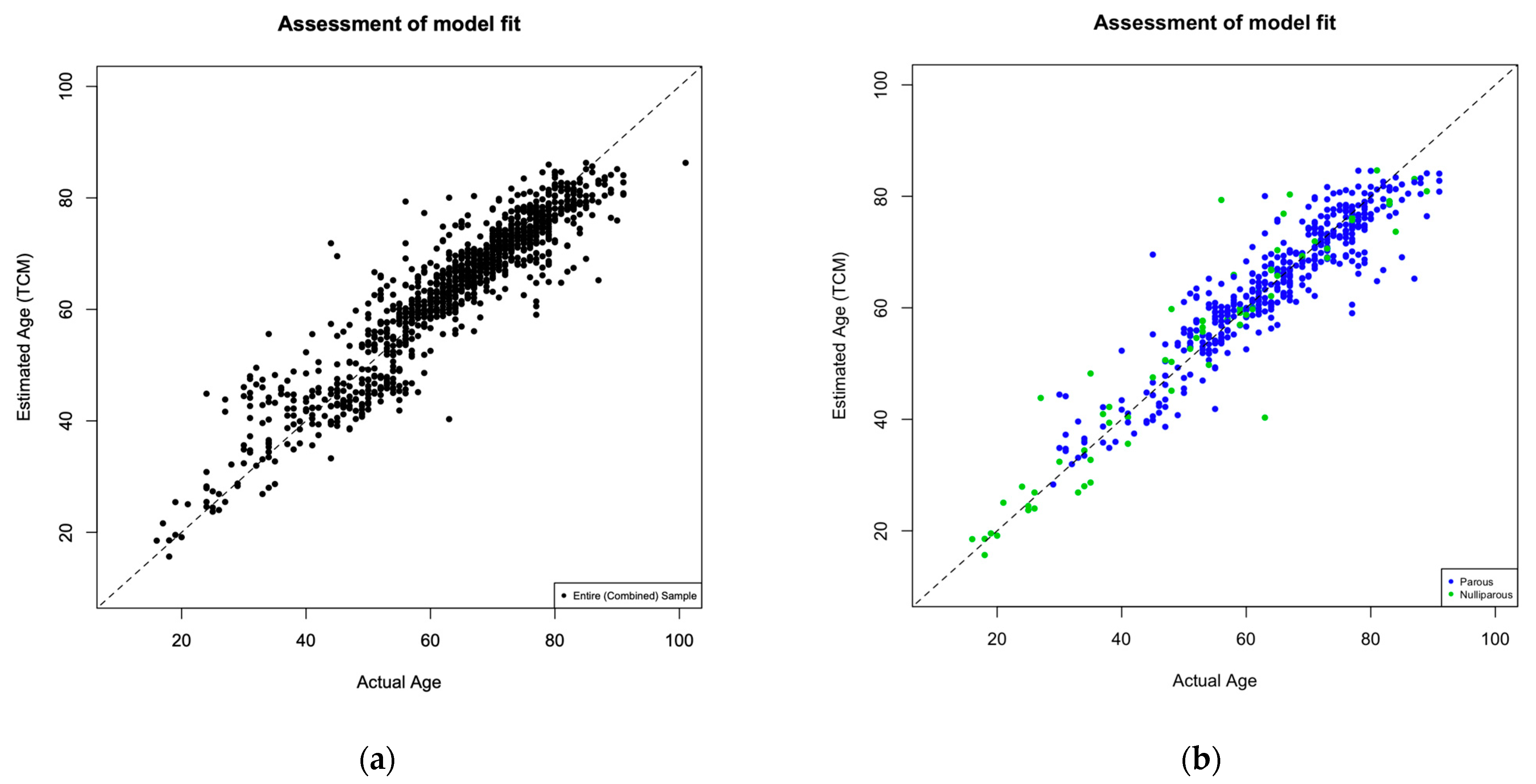
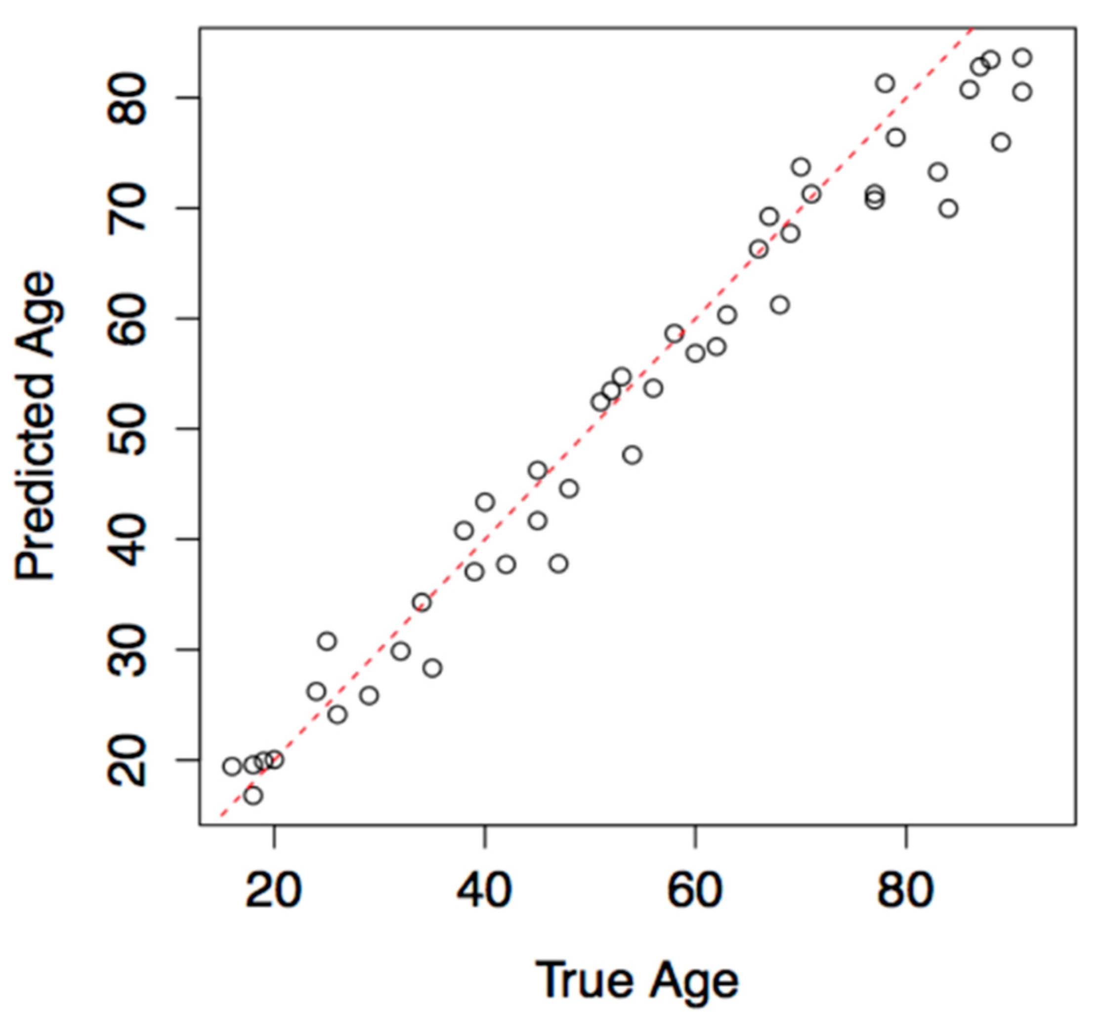
For the 533 female participants in this study, the TCM was shown to predict age reasonably well (RSME = 5.62 years, R² = 0.85, PCC = 0.92), with an overall inaccuracy of 3.86 (years) and bias of 0.69 (years) (Table 5, Figure 13).

Inaccuracy by decade ranged from 2.04 years (18–29 age group) to 7.71 years (30–39 age group). Bias by decade ranged from −0.46 years (60–69 age group) to 7.50 years (30–39 age group). Results by decade are presented in

Table 6. TCM results by decade (females).

Age Group		n =	Error	1 σ	2 σ	Inaccuracy	Bias
18–19	4	13	−0.2	2.9	5.8	2.04	1.04
20–29	9
30–39	29	29	4.3	5.7	11.4	7.71	7.50
40–49	42	42	1.7	7.2	14.4	5.35	4.63
50–59	117	117	0.1	6.3	12.6	3.71	2.32
60–69	137	137	−0.6	5.7	11.4	3.44	−0.46
70–79	149	149	−1.5	5.1	10.2	3.12	−0.84
80–89	42	46	−4.4	5.7	11.4	4.71	-3.05
90–99	4

.

4.1. Observer Subset

In addition to the author’s analysis of the entire sample, three independent observers were asked to apply the Suchey–Brooks method, the Hartnett method, and the TCM to a subset of 50 individuals (

Table 7. Results by observer and method, observer subset (n = 50).

#	Age		Author				Observer 1				Observer 2				Observer 3
			SB *	H †	TCM ‡		SB	H	TCM		SB	H	TCM		SB	H	TCM
					R §	A ((			R	A			R	A			R	A
1	18	N ¶	19.4	19.8	17.86	19	19.4	19.8	18.91	20	19.4	19.8	15.31	16	19.4	19.8	14.29	15
2	88	P **	60	82.54	86.33	87.5	60	82.54	84.32	85	60	72.34	84.32	85	60	82.54	85.13	85
3	47	P	38.2	43.26	41.76	45	48.1	51.47	54.02	52	38.2	43.26	46.64	50	38.2	43.26	53.33	51
4	29	P	25	23.2	29.53	31	25	23.2	36.38	39	30.7	43.26	38.65	41	30.7	31.44	35.69	38
5	77	N	60	72.34	76.47	76	60	82.54	70.30	69	60	72.34	76.44	76	60	82.54	73.97	73
6	93	P	60	82.54	87.24	88	60	82.54	88.94	90	60	72.34	79.21	79	60	82.54	—	—
7	35	N	30.7	31.44	31.74	34.5	25	23.2	33.35	35	30.7	31.44	30	32	25	23.2	30.87	32
8	19	N	19.4	19.8	18.67	19.5	19.4	19.8	19.49	20	19.4	19.8	19.93	21	19.4	19.8	18.91	20
9	56	P	48.1	51.47	50.52	54	48.1	51.47	46.64	50	48.1	51.47	63.70	62	60	72.34	66.18	65
10	68	P	60	72.34	57.80	61.5	60	82.54	72.15	72	60	72.34	50.74	54	60	82.54	54.62	56
11	42	P	38.2	43.26	42.83	45.5	30.7	31.44	49.98	47	38.2	43.26	50.27	48	48.1	51.47	59.47	58
12	24	N	25	23.2	19.32	25.5	30.7	31.44	37.47	34	30.7	31.44	24.55	26	30.7	31.44	27.97	30
13	71	P	60	72.34	71.46	70.5	60	82.54	73.39	73	48.1	72.34	72.05	71	60	82.54	75.20	75
14	58	P	48.1	51.47	54.89	59.5	60	82.54	53.58	51	60	72.34	56.94	55	48.1	51.47	54.89	53
15	51	N	48.1	51.47	50.37	54	60	82.54	78.22	78	48.1	72.34	71.49	71	48.1	51.47	63.07	62
16	83	N	60	82.54	78.78	79.5	60	82.54	88.94	90	60	72.34	79.60	79	60	82.54	82.77	83
17	39	P	30.7	31.44	31.78	36.5	25	23.2	20.53	21	30.7	31.44	44.54	48	25	23.2	27.97	30
18	62	N	60	72.34	58.75	61.5	48.1	51.47	71.24	70	48.1	72.34	66.71	66	48.1	72.34	53.34	51
19	91	P	60	82.54	85.38	86	60	82.54	88.94	90	60	82.54	83.25	84	60	82.54	84.32	85
20	74	N	60	82.54	75.07	75	48.1	51.47	74.21	74	48.1	72.34	67.91	67	60	82.54	—	—
21	18	N	19.4	19.8	14.29	15	19.4	19.8	14.29	15	25	23.2	15.13	16	19.4	19.8	14.73	16
22	48	N	38.2	43.26	41.12	46	30.7	31.44	44.60	42	48.1	72.34	72.42	70	—	—	—	—
23	66	P	60	72.34	62.06	66.5	60	72.34	53.59	52	60	72.34	55.02	52	48.1	72.34	67.80	67
24	26	N	25	23.2	24.06	24	25	23.2	22.26	24	30.7	31.44	30.34	32	25	23.2	24.79	26
25	86	P	60	82.54	82.06	82	60	82.54	88.94	90	60	72.34	84.32	85	60	82.54	87.88	89
26	38	N	38.2	43.26	46.01	41.5	48.1	51.47	56.97	54	48.1	72.34	71.25	73	25	23.2	62.06	62
27	91	P	60	82.54	81.66	84	60	82.54	73.98	73	48.1	72.34	62.71	60	60	82.54	88.94	90
28	53	P	48.1	51.47	48.99	53	38.2	43.26	56.44	54	48.1	72.34	65.39	64	38.2	43.26	54.89	53
29	79	P	60	72.34	76.24	75.5	60	82.54	80.24	80	60	72.34	86.02	87	60	82.54	87.87	89
30	34	N	30.7	31.44	36.78	38	38.2	43.26	32.54	35	38.2	43.26	44.33	47	25	23.2	42.02	45
31	60	P	48.1	51.47	53.11	57.5	60	72.34	66.23	65	60	72.34	79.69	80	48.1	51.47	52.78	56
32	18	N	19.4	19.8	18.47	19	25	23.2	19.93	21	19.4	19.8	19.49	20	19.4	19.8	18.47	19
33	45	P	38.2	43.26	44.76	48.5	30.7	31.44	50.24	48	48.1	72.34	69.79	69	38.2	43.26	58.64	57
34	81	N	60	82.54	71.85	78	48.1	51.47	75.63	75	60	72.34	80.49	81	60	82.54	77.73	78
35	25	N	25	23.2	23.31	24	30.7	31.44	29.72	32	48.1	51.47	25.30	28	25	23.2	23.53	25
36	32	P	30.7	31.44	33.25	36	48.1	51.47	40.77	44	48.1	51.47	60.13	58	38.2	43.26	44.56	48
37	78	P	60	82.54	82.84	83	60	82.54	82.86	84	60	82.54	79.68	80	60	82.54	—	—
38	52	N	48.1	51.47	50.87	54.5	30.7	31.44	74.05	74	48.1	72.34	64.39	64	48.1	72.34	59.70	58
39	87	P	60	82.54	84.32	85	60	82.54	85.38	86	60	82.54	81.30	81	60	82.54	88.94	90
40	20	N	19.4	19.8	19.20	20	19.4	19.8	19.97	21	25	23.2	18.95	20	25	23.2	20.99	22
41	63	P	48.1	51.47	55.75	59.5	48.1	51.47	55.58	52	38.2	43.26	60.01	58	48.1	51.47	54.50	53
42	40	P	38.2	43.26	37.77	40.5	38.2	43.26	34.90	37	48.1	51.47	46.64	50	30.7	31.44	39.76	43
43	89	N	60	82.54	82.23	82.5	60	82.54	84.82	85	60	82.54	82.28	82	60	82.54	89.45	90
44	45	N	48.1	43.26	42.33	45.5	48.1	51.47	50.67	49	48.1	72.34	62.68	60	38.2	43.26	54.64	52
45	69	P	60	72.34	68.53	68	60	82.54	53.37	51	60	72.34	69.23	68	60	72.34	66.18	65
46	54	N	38.2	43.26	55.12	53	30.7	31.44	47.17	50	38.2	43.26	56.68	54	38.2	43.26	38.08	41
47	70	P	60	72.34	75.47	75	60	82.54	78.72	79	60	72.34	79.50	80	48.1	51.47	67.82	66
48	77	N	60	72.34	75.43	75	60	72.34	74.13	74	60	72.34	84.32	85	60	82.54	81.12	81
49	67	P	60	72.34	68.95	68.5	60	82.54	70.09	70	60	72.34	70.51	70	48.1	72.34	77.79	78
50	84	N	60	72.34	76.75	76	60	72.34	76.22	76	60	72.34	76.00	75	—	—	—	—

* SB = Estimations resulting from the utilization of the Suchey–Brooks method. ^† H = Estimations resulting from the utilization of the Hartnett method. ^‡ TCM = Estimations resulting from the utilization of the TCM. ^§ R = Estimations resulting from the utilization of the TCM, regression approach. A ⁽⁽ = Estimations resulting from the utilization of the TCM, addition approach. ^¶ Indicates nulliparous. ** Indicates parous.

). This subset was curated through stratified random sampling in order to ensure that a minimum number of individuals, as well as an equal number of parous and nulliparous participants, were represented in each decade. Each observer performed his or her examinations separately, blindly, and with no prior experience with or exposure to the TCM. Each performed his or her examination on a desktop computer and examined each of the 50 scans in succession with access to multiple views, including axial, coronal, sagittal, and moveable 3D renderings. The author, Observer 1 (Ph.D.), and Observer 2 (Ph.D., Cert FA-I) performed their examinations using General Electric’s (GE) “Centricity” software, while Observer 3 (Ph.D., D-A.B.F.A., Cert FA-I) performed his or her analysis utilizing “Mimics” software by Materialize.

Subjects were placed into appropriate Suchey–Brooks ranges an average of 99% (author included) and 98% (author excluded) of the time; however, only 57% (author included) and 54% (author excluded) of the time was the mean within a decade of the individual’s actual age. Within that, only 32% (author included) and 28% (author excluded) of the time was the estimated age within five years of the actual age. Using the Hartnett method, the subjects were placed into appropriate ranges an average of 80% (author included) and 73% (author excluded) of the time, with means within 10 years of the actual age an estimated 69% (author included) and 60% (author excluded) of the time, and to within 5 years of the actual age 45% (author included) and 37% (author excluded) of the time. When applying the TCM, the subjects were placed into appropriate ranges an average of 86% (author included) and 81% (author excluded) of the time, with means within 10 years of the actual age an average of 84% (author included) and 78% (author excluded) of the time, and within 5 years an average of 65% (author included) and 57% (author excluded) of the time (

Table 8. Estimation accuracy by observer and method, observer subset (A = Author, Obs 1 = Observer 1, Obs 2 = Observer 2, Obs 3 = Observer 3, ✓? = Actual age captured within predicted range).

	Suchey-Brooks				Hartnett				Composite Method (TCM)
	✓?	<5 years	<10 years	>10 years	✓?	<5 years	<10 years	>10 years	✓?	<5 years	<10 years	>10 years
A	50/50 (100%)	20/50 (40%)	10/50 (20%)	20/50 (40%)	48/50 (96%)	35/50 (70%)	12/50 (24%)	3/50 (6%)	50/50 (100%)	46/50 (92%)	4/50 (8%)	0/50 (0%)
Obs 1	49/50 (98%)	12/50 (24%)	12/50 (24%)	26/50 (52%)	34/50 (68%)	16/50 (32%)	13/50 (26%)	21/50 (42%)	44/50 (88%)	28/50 (56%)	13/50 (26%)	9/50 (18%)
Obs 2	50/50 (100%)	17/50 (34%)	11/50 (22%)	22/50 (44%)	33/50 (66%)	20/50 (40%)	8/50 (16%)	22/50 (44%)	36/50 (72%)	24/50 (48%)	12/50 (24%)	14/50 (28%)
Obs 3	48/48 (100%)	11/48 (23%)	11/48 (23%)	26/48 (54%)	38/48 (79%)	21/48 (44%)	15/48 (31%)	12/48 (25%)	41/45 (91%)	25/45 (56%)	11/45 (24%)	9/45 (20%)

).

When compared with Suchey–Brooks, this constitutes a 33% (author included) and 29% (author excluded) increase in precision to within 10 years of actual age and a 27% (author included) and 24% (author excluded) increase in precision to within 5 years of actual age. For the Hartnett method, precision to within 10 years of actual age was increased by 15% (author included) and 19% (author excluded) and to within 5 years by 20% (both with the author included and excluded). When applying the TCM, the estimates of 10 years or more from actual age averaged 22% across all of the observers, as opposed to 32% (author included) and 40% (author excluded) when using the Hartnett method and 43% (author included) and 45% (author excluded) when using the Suchey–Brooks method. With (t-test) p-values of 0.964 (author), 0.836 (Observer 1), 0.429 (Observer 2), and 0.806 (Observer 3), no significant difference was observed between actual and estimated age when applying the TCM (

Table 9. Actual age versus estimated (mean) age by method, observer subset (females, n = 50).

	Actual Age versus Estimated (Mean) Age Using the Suchey-Brooks Method
	t	df	p	PCC	% Error	Inaccuracy	Bias
Author	2.294	75.619	0.025	0.953	−17.501	9.98	−9.49
Observer 1	2.219	76.140	0.029	0.863	−16.993	12.34	−9.22
Observer 2	1.906	70.163	0.061	0.848	−14.052	12.05	−7.60
Observer 3	2.626	74.679	0.011	0.933	−19.914	12.42	−9.78
	Actual Age versus Estimated (Mean) Age Using the Hartnett Method
	t	df	p	PCC	% Error	Inaccuracy	Bias
Author	0.353	87.906	0.725	0.979	−3.139	4.07	−1.70
Observer 1	−0.097	87.679	0.923	0.868	0.903	9.88	0.49
Observer 2	−0.813	86.081	0.418	0.833	6.859	10.54	3.76
Observer 3	0.131	87.805	0.896	0.932	−1.214	7.23	−0.61
	Actual Age versus Estimated (Mean) Age Using The Composite Method
	t	df	p	PCC	% Error	Inaccuracy	Bias
Author	0.075	87.447	0.964	0.989	−0.389	2.66	−0.19
Observer 1	−0.208	87.888	0.836	0.919	1.843	5.98	1.00
Observer 2	−0.793	87.349	0.429	0.876	6.882	8.26	3.73
Observer 3	−0.247	87.971	0.806	0.941	2.212	6.04	1.17

).

Echoing the results of the author’s analysis of the entire sample (Table 4), application preference (regression or addition) again demonstrated no meaningful effect on estimation accuracy or reliability amongst the three observers (

Table 10. T-test and Pearson coefficient analyses comparing estimates derived by regression versus simple addition.

		Actual Age v Regression Estimates				Actual Age v Addition Estimates				Regression v Addition Estimates
	n=	t	df	p	PCC	t	df	p	PCC	t	df	p	PCC
All Females	533	−0.0607	1057.2	0.9516	0.9245	−0.6081	1051.3	0.5433	0.9251	−0.5706	1063.0	0.5684	0.9953
Author	50	0.4918	87.825	0.6241	0.98783	0.1263	87.685	0.8998	0.9934	−0.3778	87.979	0.7065	0.9950
Observer 1	50	−0.2316	87.983	0.8174	0.9179	−0.2214	87.922	0.8253	0.9179	0.0121	87.978	0.9904	0.9968
Observer 2	50	−0.7591	87.761	0.4498	0.8776	−0.8066	87.479	0.4221	0.8731	−0.0396	87.945	0.9685	0.9969
Observer 3	45	−0.2984	88	0.7661	0.9399	−0.3359	87.944	0.7377	0.9399	−0.0338	87.944	0.9731	0.9969

).

4.2. Inter-Observer Error

Inter-observer agreement was mixed with the author—who had extensive previous experience with both the TCM and medical imaging more generally—predictably performing the best. By contrast, none of the three observers had seen the TCM before, having been introduced to it on the day of their first session. Furthermore, none of the observers were familiar with working virtually, having worked only with physical bone in the past. For these reasons, the results have been presented both with and without the author, for additional perspective.

Agreement was measured through two tailed t-tests, Pearson’s coefficient, and chi-squared analysis (

Table 11. Inter-observer comparisons by estimation method, observer subset (females, n = 50).

	Suchey-Brooks					Hartnett					TCM
	t	df	p	PCC	X2 (p)	t	df	p	PCC	X2 (p)	t	df	p	PCC	X2 (p)
Author v Obs 1	−0.086	87.988	0.932	0.903	0.000	−0.439	87.246	0.661	0.878	0.035	−0.262	87.830	0.794	0.932	0.487
Author v Obs 2	−0.622	86.644	0.536	0.896	0.000	−1.207	86.807	0.231	0.857	0.392	−0.874	87.996	0.385	0.892	0.454
Author v Obs 3	0.414	87.960	0.679	0.929	0.005	−0.211	87.446	0.833	0.942	0.229	−0.302	87.669	0.764	0.949	0.644
Obs 1 v Obs 2	−0.526	86.384	0.600	0.894	0.000	−0.681	84.352	0.498	0.831	0.912	−0.592	87.774	0.555	0.907	0.197
Obs 1 v Obs 3	0.498	87.903	0.619	0.854	0.000	0.222	87.984	0.825	0.822	0.925	−0.042	87.973	0.967	0.924	0.017
Obs 2 v Obs 3	1.069	87.058	0.288	0.837	0.015	0.931	84.775	0.355	0.799	0.261	0.544	87.593	0.588	0.906	0.053

). When applying the Suchey–Brooks method, all of the observers’ results (estimated ranges capturing the actual age, in this case) agreed, whereas only the author and Observer 1 agreed when applying the Hartnett method (X² p = 0.035). There was agreement (X² p = 0.017) between Observer 1 and Observer 3 when applying the TCM, with borderline agreement (X² p = 0.053) between Observer 2 and Observer 3.

This overall pattern was echoed by the subset’s Fleiss’ Kappa scores [82,83], by which the Suchey–Brooks method exhibited the highest degree of agreement, the Hartnett method exhibited the lowest degree of agreement, and the TCM exhibited a level of mixed agreement falling between the two (

Table 12. Fleiss’ Kappa comparisons by estimation method, observer subset (females, n = 50).

		Suchey-Brooks	Hartnett	TCM
Including Author		0.75 (95% CI), p = 0	0.12 (95% CI), p = 0.0562	0.16 (95% CI), p = 0.00698
		Moderate Agreement	No Agreement	No Agreement
Excluding Author		0.68 (95% CI), p = 2.44 × 1015	0.16 (95% CI), p = 0.067	0.30 (95% CI), p = 0.000551
		Moderate Agreement	No Agreement	Minimal Agreement

).

4.3. Cross Validation

In order to investigate the validity and the robusticity of the model’s predictive element, the observer’s subset was additionally eliminated from the dataset and the model was re-fitted without it. The TCM regression was then used to predict the ages of the “unknown” subjects. The results were plotted as a graph of “predicted“ (estimated) age versus “true” (actual) age for a visual assessment of how well the model performed (Figure 14).

5. Application Example

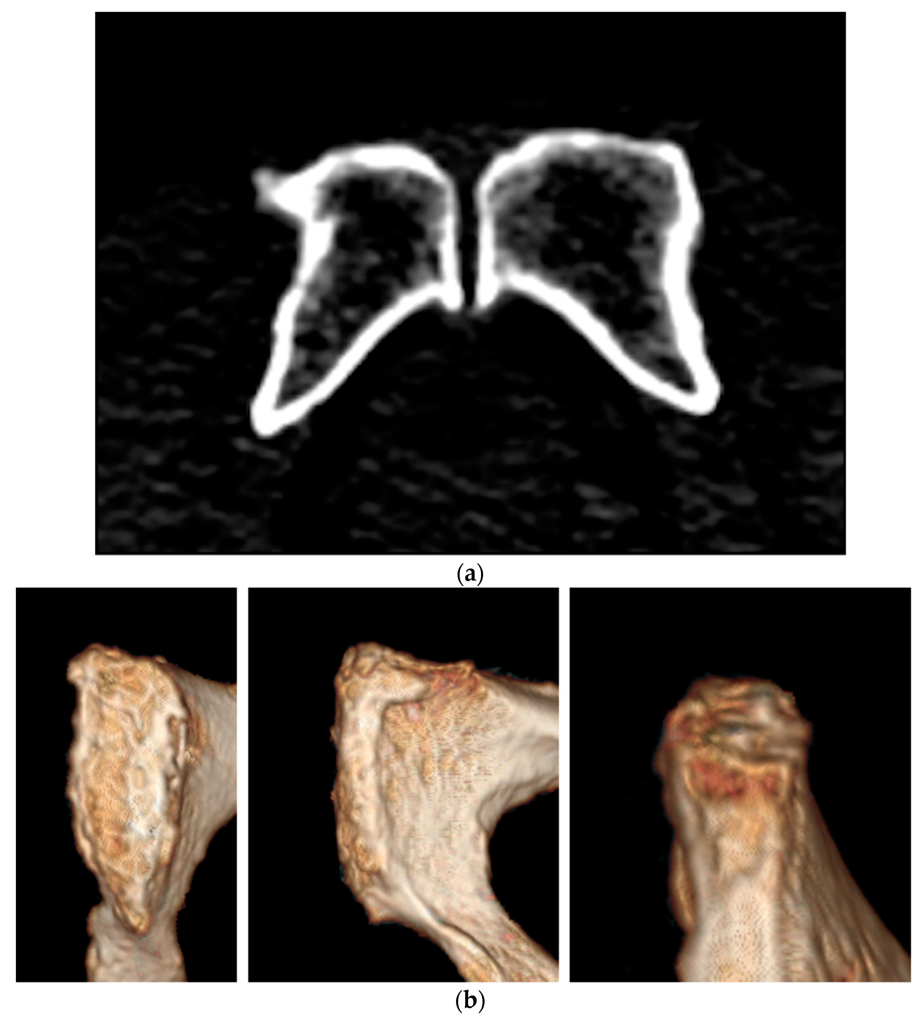
By examining the individual represented in Figure 15a,b, both applications of the TCM may be illustrated.

It is the author’s preference to begin with density, therefore the axial image for this individual will be examined first (Figure 15a). As can be seen, the articulation’s cortical bone appears bright white and uniform, but has noticeably thinned at various points along the ventral margin, creating breaches in the line and the appearance of “islands” or “pearls” of opacity within the broken border. Inside, the trabecular space presents as approximately 50% gray and 50% black. No pathology or artifact is observed. The adjustment for this individual would therefore be medium and a score of five would be noted.

Moving next to the Upper Boundary (Figure 2 and Figure 3), it is apparent from the axial image that the UB has “squared off” (the wide, softly curved “V” shape that once existed in the space between the two faces has closed to create more of a “Y” or “T” shape), reflecting the completion and cessation of epiphyseal activity in that area. This indicates that anything below a score of seven may be immediately discounted.

Next, by comparing the image in question (Figure 15b) to the stylized illustrations and rendered images, it can be seen that a distinct border does exist at the UB and is not swelled or smooth but has instead thinned quite severely, broken in several places, and become irregular. The face and tubercle also exist as two disparate entities and large macro-pores have begun to erode the surface. For the Upper Boundary, therefore, a score of 15 would be appropriate for this individual.

The same process may be applied to the Lower Boundary (Figure 4 and Figure 5), where an eroded convexity exists within a broken, erratic border. A score of 16 would best fit this individual.

Moving through to the Outline (Figure 6 and Figure 7), it may be seen that the border, as a whole, has thinned, broken in several places, and taken on a rough, irregular shape. A score of 15 would again best represent this individual.

Surface Texture (Figure 8 and Figure 9) appears to be a mix of smoothness (white or tan) and degradation (dark brown or red) in the form of macro-pore erosion. Given this, a score of 14 would be most appropriate for this individual.

Lastly, Topography (Figure 10 and Figure 11) exhibits a slightly rounded convexity of the entire surface, but with disorganized, haphazard erosion instead of uniform ridges and furrows. A score of 16 would be the best match.

For this individual, therefore, the summed scores would be 5 (Density), 15 (UB), 16 (LB), 15 (Outline), 14 (Surface Texture), and 16 (Topography). As 5 + 15 + 16 + 15 + 14 + 16 = 81, the estimated age for this individual via the simple addition approach would be 81 years ± 12, or 69 to 93 years.

Following the regression approach, the computation would be as follows:

−1.99 + (3.01 × 2.24) + (0.92 × 15) + (0.46 × 16) + (1.13 × 15) + (1.18 × 14) + (1.38 × 16) =

which becomes:

−1.99 + 6.74 + 13.8 + 7.36 + 16.95 + 16.52 + 22.08 = 81.46

At a 95% confidence interval with a standard deviation of 5.66, the estimated range for this individual would be 81.46 years ± 11.32, or 70.14 to 92.78 years.

At the time of her scan, the age of the individual represented in Figure 15a,b was 79 years.

6. Discussion

Despite renewed scholarship steadily raising range and transition thresholds elsewhere around the body, the long-held belief that “changes on the pubic symphysis are observed up to 40 years of age, after which the pubic symphysis does not show any changes usable for age estimation” [84] (p. 172) remains deeply ingrained. The results from this study did not support this view.

When the data were evaluated as a whole, inaccuracy and bias were consistently lower for those who were aged 50–99 years than for those aged 30–49 years. As would be expected, due to epiphyseal activity, individuals aged 18–29 years presented the lowest inaccuracy (Table 6). The fact that this pattern emerged is unsurprising, given the absence of axiomatic change during the stasis period between build-up (scores 3–8, roughly 15 to 40 years) and breakdown (scores 11–16, roughly 55 to 80 years). That the difference in inaccuracy between the “under 50s” (combined) and the “over 50s” (combined) was negligible (15.1 versus 14.98), however, was surprising as, despite individual genetic expression, life history, and environment having had more time to act upon the older participants [2,3,4,5,6,7,85,86,87,88,89], degenerative change in this study appeared to be no more unreliable or unpredictable than was generative change.

When taken separately, the left pubic face (t(1039) = −0.1865; p = 0.2357 [CI 95%], inaccuracy = 3.996, bias = 1.124) performed slightly better when compared with actual age than did the right (t(1028.8) = −0.96119; p = 0.3367 [CI 95%], inaccuracy = 4.400, bias = 0.118); however, when both were present, an averaging of the two (t(1051.6) = −0.69564; p = 0.4868 [CI 95%], inaccuracy = 3.865, bias = 0.691) outperformed either side individually. While this contradicts the previous literature (52), it is recommended that, when possible, both sides be evaluated and averaged in order to obtain the best results when applying the TCM.

There was also no significant difference between estimated age and actual age when calculating scores by means of linear regression (t(1057.2) = −0.0607; p = 0.9245 [CI 95%]) and simple addition (t(1051.3) = −0.6081; p = 0.9251 [CI 95%]) (Table 3). Whether to input the scores into an equation, or to simply add them for an immediate estimate, therefore, remains a matter of personal need and preference.

This study’s use of a hospital sample should also be addressed. Often, hospital samples are viewed as somewhat suspect and are dismissed as both pathological and self-selecting. While it is true that this sample was broadly self-selecting, the participants were scanned for any number of reasons and neither chronic (cancer management or the monitoring of an abdominal aortic aneurism, for example) nor acute (urinary tract infection, kidney or bladder stones, or pre-surgical planning, for example) conditions were shown to affect age estimation in this cohort (Table 2).

In this sample, stepwise changes in density were not distinct enough to accommodate 14 individual scores, and it was therefore divided into three larger categories (0, 5, and 10) instead. A continuum that was similar to the other AOIs was trialed (allowing for scores of three or eight, for example) but was discontinued in the wake of marginally increased inaccuracy. In placing more distance between the three images, subtle gradations became more pronounced, making them easier to see and identify. This was not the case for the other AOIs, as progressive change did prove discrete enough for a more detailed analysis. Because it was condensed while the other AOIs were not, and because it required additional information that was facilitated by an alternate view (axial images), density was considered to be an adjustment as opposed to a sixth AOI. Due to the time constraints of the thesis upon which this work was based, this could not be further refined. However, while beyond the scope of the project at the time, expanding density to fit the format of the other AOIs and/or quantifying it in a more systematic way, such as by Hounsfield Unit [90,91,92], remains an avenue of future research that could only benefit subsequent estimations.

Additional limitations center around the TCM’s virtual medium. Practitioners who are unfamiliar with 3D visualization may find the elimination of physical tactility more difficult than those who are more experienced with virtual platforms. Likewise, those who are unable to differentiate between the subtle shifts in color hue or intensity may also find visual texture analysis challenging. Solutions to this could include standardizing “depth” through CIELAB coordinates [93] or through the creation of an automated Munsell-like [94] color-comparison scale.

No significant difference has been shown to exist between clinical CT (individuals who were alive at their time of scan) and either post-mortem CT or physical bone, leading to multiple symphysis-specific studies combining and discussing the three mediums interchangeably [95,96,97,98,99]. This method may, likewise, be utilized with equal confidence for both living and post-mortem CT assessments. As this study was undertaken in partnership with living volunteers, however, the limitations that are often associated with estimation from the pubic symphysis were circumvented in that the faces were not affected by missing elements (ossific nodules displaced by soft tissue loss, for example), compromised preservation, or obscuring taphonomy. Therefore, until additional studies can be performed, the TCM cannot be recommended for the assessment of non-fleshed remains (especially those that are believed to be 25 years or younger).

Finally, the Oxford, UK, based sample that was utilized for this study (predominantly Caucasian and predominantly mid to high socio-economic status) yielded an estimation envelope of 22.64 years by regression and 24 years for addition. This may not be the case for other groups. Until further research can be undertaken to either confirm the applicability or to establish new envelopes as needed, caution should be exercised when applying the TCM to populations of differing backgrounds and life history.

7. Conclusions

In this study, the TCM returned lower error rates, lower RSME and MAE values, lower inaccuracy, and lower bias than the more “advanced” methods, but without the need for specialized training, dedicated equipment, or complex software. In 2009, Cunha et al. [9] (p. 3) stated that “sometimes the best methods are not those with the best published standard error” but those “which are suitable for a specific forensic scenario, practical, user-friendly, relatively quick and cheap.” For the individuals in this sample, the TCM proved to be both.

The US Census Bureau projects that, as current “baby boomers” transition into the “oldest-old” age category, nearly one in five Americans will reach 65 or older not by 2050 as posited by the United Nations, but by 2030 [34]. With predictions such as these, it is increasingly important that the field comes to better terms with age estimation in older individuals. The issues of migration and the Rights of the Child have intensified efforts regarding estimation for minors; however, while that focus is much needed, the young are not the only demographic to experience displacement and are not the only ones who are entitled to care based upon age. Many older individuals rely on pensions or dispensations for their healthcare and day to day expenses. When birth certificates or other identifying documentation are lost or unavailable, funds and services become inaccessible at a time of life when they are often needed the most. Older individuals are also more likely to go missing due to age-related ailments such as Alzheimer’s dementia, which affects one in nine seniors and is the sixth leading cause of death in the United States [100]. Equally, natural disasters, such as floods, wildfires, and earthquakes, have been shown to affect older populations disproportionately [101,102,103], while human disasters, such as crashes, collapses, conflict, and acts of terrorism, do not discriminate by age.

Despite excellent recent work undertaken to investigate alterations in pubic bone shape and structure through cutting edge technological advances [46,69,72,84,104,105,106,107], estimation imprecision for those “over 50” remains relatively unchanged. Instead of focusing on morphology, this research concentrated on degenerative change as a distinguishing feature in itself—not as an indiscriminate destructive force, but as the natural continuation of an ongoing process. It is hoped that by better understanding the diagnostic value of the subtleties of senescent change, age estimation in mature adults may be improved.

References

- Milner, G.R.; Boldsen, J.L. Skeletal Age Estimation: Where We Are and Where We Should Go. In A Companion to Forensic Anthropology; Dirkmaat, D.C., Ed.; Wiley Blackwell Publishing: West Sussex, UK, 2012; pp. 224–238. [Google Scholar]
- Kemkes-Grottenthaler, A. Aging Through the Ages: Historical Perspectives on Age Indicator Methods. In Paleodemography: Age Distributions from Skeletal Samples; Hoppa, R., Vaupel, J., Eds.; Cambridge University Press: Cambridge, UK, 2002; pp. 48–72. [Google Scholar]
- Kobyliansky, E.; Karasik, D.; Belkin, V.; Livshits, G. Bone Ageing: Genetics Versus Environment. Ann. Hum. Biol. 2000, 27, 433–451. [Google Scholar] [PubMed]
- Mays, S. The Effect of Factors Other Than Age Upon Skeletal Age Indicators in the Adult. Ann. Hum. Biol. 2015, 42, 332–341. [Google Scholar] [CrossRef] [PubMed]
- Langley, N.R.; Jantz, R.L.; Ousley, S.D. The Effect of Novel Environments on Modern American Skeletons. Hum. Biol. 2016, 88, 5–13. [Google Scholar] [CrossRef] [PubMed]
- Truesdell, J.M. Improving Precision in Age Estimation from the Female Pubic Symphysis: A Novel Technique for CT. Ph.D. Thesis, University of Oxford, Oxford, UK, 2017. [Google Scholar]
- Schmitt, A. Variabilité de la sénescence du squelette humain—Réflexions sur les indicateurs de l’âge au décès: À la recherché d’un outil performant. Ph.D. Thesis, University of Bordeaux, Bordeaux, France, 2001. [Google Scholar]
- Buckberry, J. The (Mis)Use of Adult Age Estimates in Osteology. Ann. Hum. Biol. 2015, 42, 323–331. [Google Scholar] [CrossRef] [Green Version]
- Cunha, E.; Baccino, E.; Martrille, L.; Ramsthaler, F.; Prieto, J.; Schuliar, Y.; Lynnerup, N.; Cattaneo, C. The Problem of Aging Human Remains and Living Individuals: A Review. Forensic Sci. Int. 2009, 193, 1–13. [Google Scholar] [CrossRef]
- Cappella, A.; Cummaudo, M.; Arrigoni, E.; Collini, F.; Cattaneo, C. The Issue of Age Estimation in a Modern Skeletal Population: Are Even the More Modern Current Aging Methods Satisfactory for the Elderly? J. Forensic Sci. 2017, 62, 12–17. [Google Scholar] [CrossRef]
- Falys, C.G.; Lewis, M.E. Proposing a Way Forward: A Review of Standardisation in the Use of Age Categories and Ageing Techniques in Osteological Analysis (2004–2009). Int. J. Osteoarchaeol. 2010, 21, 704–716. [Google Scholar] [CrossRef]
- Merritt, C. Testing the Accuracy of Adult Skeletal Age Estimation Methods: Original Methods Versus Revised and Newer Methods. Vis. Exp. Anthr. 2013, 12, 102–119. [Google Scholar]
- Baccino, E.; Schmitt, A. Determination of Adult Age at Death in the Forensic Context. In Forensic Anthropology and Medicine: Complementary Sciences from Recovery to Cause Death; Schmitt, A., Cunha, E., Pinheiro, J., Eds.; Humana Press Inc.: Totowa, NJ, USA, 2006; pp. 259–280. [Google Scholar]
- Falys, C.G.; Prangle, D. Estimating Age of Mature Adults from the Degeneration of the Sternal End of the Clavicle. Am. J. Phys. Anthr. 2015, 156, 203–214. [Google Scholar] [CrossRef] [Green Version]
- Price, M. Age Estimation Using the Sternal End of the Clavicle: A Test of the Falys and Prangle (2014) Archaeological Method for Forensic Application. Master’s Thesis, Boston University, Boston, MA, USA, 2017. [Google Scholar]
- Blom, A.A.; Inskip, S.A.; Baetsen, W.A.; Hoogland, M.L.P. Testing the Sternal Clavicle Aging Method on a Post-Medieval Dutch Skeletal Collection. Archaeometry 2018, 60, 1391–1402. [Google Scholar] [CrossRef]
- Falys, C. Estimating Age of Mature Adults from the Degeneration of the Ischial Tuberosity. In Proceedings of the 55th Annual Society for the Study of Human Biology Symposium, Oxford, UK, 9–11 December 2014. [Google Scholar]
- DiGangi, E.A.; Bethard, J.D.; Kimmerle, E.H.; Konigsberg, L.W. A New Method for Estimating Age-at-Death from the First Rib. Am. J. Phys. Anthr. 2009, 138, 164–176. [Google Scholar] [CrossRef] [PubMed]
- Sullivan, Z. Use of the First Rib in the Age-at-Death Assessment of Adult Female Skeletal Remains. Master’s Thesis, Western Washington University, Bellingham, WA, USA, 2012. [Google Scholar]
- Hartnett, K. Analysis of Age-at-Death Estimation Using Data from a New, Modern Autopsy Sample--Part II: Sternal End of the Fourth Rib. J. Forensic Sci. 2010, 55, 1152–1156. [Google Scholar] [CrossRef] [PubMed]
- Merritt, C. A Test of Hartnett’s Revisions to the Pubic Symphysis and Fourth Rib Methods on a Modern Sample. J. Forensic Sci. 2014, 59, 703–711. [Google Scholar] [CrossRef] [PubMed]
- Buckberry, J.; Chamberlain, A. Age Estimation from the Auricular Surface of the Ilium: A Revised Method. Am. J. Phys. Anthr. 2002, 119, 231–239. [Google Scholar] [CrossRef]
- Falys, C.; Schutkowski, H.; Weston, D.A. Auricular Surface Aging: Worse than Expected? A Test of the Revised Method on a Documented Historic Skeletal Assemblage. Am. J. Phys. Anthr. 2006, 130, 508–513. [Google Scholar] [CrossRef]
- Hens, S.M.; Godde, K. Auricular Surface Aging: Comparing Two Methods that Assess Morphological Change in the Ilium with Bayesian Analyses. J. Forensic Sci. 2015, 61 (Suppl. S1), 30–38. [Google Scholar] [CrossRef]
- Calce, S. A New Method to Estimate Adult Age-at-Death Using the Acetabulum. Am. J. Phys. Anthr. 2012, 148, 11–23. [Google Scholar] [CrossRef]
- San-Millán, M.; Rissech, C.; Turbón, D. New Approach to Age Estimation of Male and Female Adult Skeletons Based on the Morphological Characteristics of the Acetabulum. Int. J. Leg. Med. 2017, 131, 501–525. [Google Scholar] [CrossRef]
- Baccino, E.; Sinfield, L.; Colomb, S.; Baum, T.P.; Martrille, L. Technical note: The Two Step Procedure (TSP) for the Determination of Age at Death of Adult Human Remains in Forensic Cases. Forensic Sci. Int. 2014, 244, 247–251. [Google Scholar] [CrossRef]
- Brennaman, A.L.; Love, K.R.; Bethard, J.D.; Pokines, J.T. A Bayesian Approach to Age-at-Death Estimation from Osteoarthritis of the Shoulder in Modern North Americans. J. Forensic Sci. 2017, 62, 573–584. [Google Scholar] [CrossRef]
- Harth, S.; Obert, M.; Ramsthaler, F.; Reuß, C.; Traupe, H.; Verhoff, M.A. Ossification Degrees of Cranial Sutures Determined with Flat-Panel Computed Tomography: Narrowing the Age Estimate with Extrema. J. Forensic Sci. 2010, 55, 690–694. [Google Scholar] [CrossRef] [PubMed]
- Watanabe, S.; Terazawa, K. Age Estimation from the Degree of Osteophyte Formation of Vertebral Columns in Japanese. Leg. Med. 2006, 8, 156–160. [Google Scholar] [CrossRef] [PubMed]
- Listi, G.A.; Manhein, M.H. The Use of Vertebral Osteoarthritis and Osteophytosis in Age Estimation. J. Forensic Sci. 2012, 57, 1537–1540. [Google Scholar] [CrossRef] [PubMed]
- Beauthier, J.-P.; Lefevre, P.; Meunier, M.; Orban, R.; Polet, C.; Werquin, J.-P.; Quatrehomme, G. Palatine Sutures as Age Indicator: A Controlled Study in the Elderly. J. Forensic Sci. 2010, 55, 153–158. [Google Scholar] [CrossRef] [PubMed]
- United Nations, Department of Economic and Social Affairs. World Population Prospects 2019: Ten Key Findings; Population Division: New York, NY, USA, 2019; pp. 1–2. [Google Scholar]
- Vincent, G.; Velkoff, V. The Next Four Decades: The Older Population in the United States—2010 to 2050; U.S. Census Bureau: WA, USA, 2010; pp. 25–1138. [Google Scholar]
- Garvin, H.M.; Passalacqua, N.V. Current Practices by Forensic Anthropologists in Adult Skeletal Age Estimation. J. Forensic Sci. 2012, 57, 427–433. [Google Scholar] [CrossRef] [PubMed]
- Todd, T.W. Age Changes in the Pubic Bone. I. The Male White Pubis. Am. J. Phys. Anthr. 1920, 3, 285–339. [Google Scholar] [CrossRef]
- Todd, T. Age Changes in the Pubic Bone, II: Pubis of the Male Negro-White Hybrid, III: Pubis of the White Female, IV: Pubis of the Female Negro-White Hybrid. Am. J. Phys. Anthr. 1921, 4, 1–77. [Google Scholar] [CrossRef] [Green Version]
- Brooks, S.T. Skeletal Age at Death: The Reliability of Cranial and Pubic Age Indicators. Am. J. Phys. Anthr. 1955, 13, 567–597. [Google Scholar] [CrossRef]
- McKern, T.W.; Stewart, T.D. Skeletal Age Changes in Young American Males, Analyzed from the Standpoint of Age Identification. In Headquarters Quartermaster Research and Development Command; Natick, MA, USA, 1957. [Google Scholar]
- Gilbert, B.M.; McKern, T.W. A Method for Aging the Female Os Pubis. Am. J. Phys. Anthr. 1973, 38, 31–38. [Google Scholar] [CrossRef]
- Hanihara, K.; Suzuki, T. Estimation of Age from the Pubic Symphysis by Means of Multiple Regression Analysis. Am. J. Phys. Anthr. 1978, 48, 233–240. [Google Scholar] [CrossRef]
- Snow, C.C. Equations for Estimating Age at Death from the Pubic Symphysis: A Modification of the McKern-Stewart Method. J. Forensic Sci. 1983, 28, 864–870. [Google Scholar] [CrossRef]
- Meindl, R.S.; Lovejoy, C.O.; Mensforth, R.P.; Walker, R.A. A Revised Method of Age Determination Using the Os Pubis with a Review and Tests of Accuracy of Other Current Methods of Pubic Symphyseal Aging. Am. J. Phys. Anthr. 1985, 68, 29–45. [Google Scholar] [CrossRef] [PubMed]
- Jackes, M.K. Pubic Symphysis Age Distributions. Am. J. Phys. Anthr. 1985, 68, 281–299. [Google Scholar] [CrossRef] [PubMed]
- Brooks, S.T.; Suchey, J.M. Skeletal Age Determination Based on the Os Pubis: A Comparison of the Ascaadi-Nemeskeri and Suchey-Brooks Methods. J. Hum. Evol. 1990, 5, 227–238. [Google Scholar] [CrossRef]
- Pasquier, E.; de Saint Martin Pernot, L.; Burdin, V.; Mounayer, C.; Le Rest, C.; Colin, D.; Mottier, D.; Roux, C.; Baccino, E. Determination of Age at Death: Assessment of an Algorithm of Age Prediction Using Numerical Three-Dimensional CT Data from Pubic Bones. Am. J. Phys. Anthr. 1999, 108, 261–268. [Google Scholar] [CrossRef]
- Boldsen, J.L.; Milner, G.R.; Konigsberg, L.W.; Wood, J.W. Transition Analysis: A New Method for Estimate Age from Skeletons. In Paleodemography: Age Distributions from Skeletal Samples; Hoppa, R., Vaupel, J.W., Eds.; Cambridge University Press: Cambridge, UK, 2002; pp. 73–107. [Google Scholar]
- Kimmerle, E.H.; Konigsberg, L.W.; Jantz, R.L.; Baraybar, J.P. Analysis of Age-at-Death Estimation through the Use of Pubic Symphyseal Data. J. Forensic Sci. 2008, 53, 558–568. [Google Scholar] [CrossRef] [PubMed]
- Chen, X.; Zhang, Z.; Zhu, G.; Zhu, G.; Tao, L. Determination of Male Age at Death in Chinese Han Population: Using Quantitative Variables Statistical Analysis from Pubic Bones. Forensic Sci. Int. 2008, 175, 36–43. [Google Scholar] [CrossRef] [PubMed]
- Chen, X.; Zhang, Z.; Zhu, G.; Tao, L. Determination of Female Age at Death in Chinese Han Population: Using Quantitative Variables Statistical Analysis from Pubic Bones. Forensic Sci. Int. 2011, 210, 278.e1–278.e8. [Google Scholar] [CrossRef]
- Fleischman, J.M. A Comparative Assessment of the Chen et al. and Suchey-Brooks Pubic Aging Methods on a North American Sample. J. Forensic Sci. 2013, 58, 311–323. [Google Scholar] [CrossRef]
- Overbury, R.S.; Cabo, L.L.; Dirkmaat, D.C.; Symes, S.A. Asymmetry of the Os Pubis: Implications for the Suchey-Brooks Method. Am. J. Phys. Anthr. 2009, 139, 261–268. [Google Scholar] [CrossRef]
- Lungmus, E.K. An Examination of Error in the Application of Pubic Aging Techniques. Master’s Thesis, University of Montana, Missoula, MT, USA, 2009. [Google Scholar]
- Berg, G.E. Pubic Bone Age Estimation in Adult Women. J. Forensic Sci. 2008, 53, 569–577. [Google Scholar] [CrossRef] [PubMed]
- Hartnett, K.M. Analysis of Age-at-Death Estimation Using Data from a New, Modern Autopsy Sample—Part 1: Pubic Bone. J. Forensic Sci. 2010, 55, 1145–1151. [Google Scholar] [CrossRef] [PubMed]
- Alcaraz, M. Análisis de Imagen Para Determinación de Edad y Sexo en Pubis, en una Muestra de Tomografía Axial Computarizada de Sujetos Adultos Vivos; Universidad de Granada: Granada, Spain, 2012. [Google Scholar]
- Godde, K.; Hens, S.M. Age-at-Death Estimation in an Italian Historical Sample: A Test of the Suchey-Brooks and Transition Analysis Methods. Am. J. Phys. Anthr. 2012, 149, 259–265. [Google Scholar] [CrossRef] [PubMed]
- Lottering, N.; MacGregor, D.M.; Meredith, M.; Alston, C.L.; Gregory, L.S. Evaluation of the Suchey-Brooks Method of Age Estimation in an Australian Subpopulation Using Computed Tomography of the Pubic Symphyseal Surface. Am. J. Phys. Anthr. 2013, 150, 386–399. [Google Scholar] [CrossRef] [Green Version]
- Chiba, F.; Makino, Y.; Motomura, A.; Inokuchi, G.; Torimitsu, S.; Ishii, N.; Kubo, Y.; Abe, H.; Sakuma, A.; Nagasawa, S.; et al. Age Estimation by Quantitative Features of Pubic Symphysis Using Multi-Detector Computed Tomography. Int. J. Leg. Med. 2014, 128, 667–673. [Google Scholar] [CrossRef]
- Sussman, R. A Comparison of Pubic Symphysis Aging Methods to Analyze Elderly Female Individuals in the Lisbon Skeletal Collection; Boston University: Boston, MA, USA, 2015. [Google Scholar]
- Castillo, A.; Galtés, I.; Crespo, S.; Jordana, X. Technical Note: Preliminary Insight into a New Method for Age-at-Death Estimation from the Pubic Symphysis. Int. J. Leg. Med. 2021, 135, 929–937. [Google Scholar] [CrossRef]
- Corsini, M.-M.; Schmitt, A.; Bruzek, J. Aging Process Variability on the Human Skeleton: Artificial Network as an Appropriate Tool for Age at Death Assessment. Forensic Sci. Int. 2005, 148, 163–167. [Google Scholar] [CrossRef]
- Morante, G.B.; Bookstein, F.L.; Fischer, B.; Schaefer, K.; Aguilera, I.A.; López, M.C.B. Correlation of the Human Pubic Symphysis Surface with Age-at-Death: A Novel Quantitative Method Based on a Bandpass Filter. Int. J. Leg. Med. 2021, 60, 835–843. [Google Scholar] [CrossRef]
- Martins, R.; Oliveira, P.E.; Schmitt, A. Estimation of Age at Death from the Pubic Symphysis and the Auricular Surface of the Ilium Using a Smoothing Procedure. Forensic Sci. Int. 2012, 219, 287.e1–287.e7. [Google Scholar] [CrossRef]
- Dudzik, B.; Langley, N. Estimating Age from the Pubic Symphysis: A New Component-Based System. Forensic Sci. Int. 2015, 257, 98–105. [Google Scholar] [CrossRef]
- Schmitt, A. Une Nouvelle Méthode Pour Discriminer les Individus Décédés avant ou Après 40 Ans à Partir de la Symphyse Pubienne. J. Med. Leg. Droit Med. 2008, 51, 15–24. [Google Scholar]
- Merritt, C. Part II-Adult Skeletal Age Estimation Using CT Scans of Cadavers: Revision of the Pubic Symphysis Methods. J. Forensic Radiol. Imaging 2018, 14, 50–57. [Google Scholar] [CrossRef]
- Buk, Z.; Kordik, P.; Bruzek, J.; Schmitt, A.; Snorek, M. The Age at Death Assessment in a Multi-Ethnic Sample of Pelvic Bones Using Nature-Inspired Data Mining Methods. Forensic Sci. Int. 2012, 220, 294.e1–294.e9. [Google Scholar] [CrossRef] [PubMed]
- Stoyanova, D.K.; Algee-Hewitt, B.F.B.; Kim, J.; Slice, D.E. A Computational Framework for Age-at-Death Estimation from the Skeleton: Surface and Outline Analysis of 3D Laser Scans of the Adult Pubic Symphysis. J. Forensic Sci. 2017, 62, 1434–1444. [Google Scholar] [CrossRef]
- Kotěrová, A.; Velemínská, J.; Cunha, E.; Brůžek, J. A Validation Study of the Stoyanova et al. Method (2017) for Age-at-Death Estimation Quantifying the 3D Pubic Symphyseal Surface of Adult Males of European Populations. Int. J. Leg. Med. 2019, 133, 603–612. [Google Scholar] [CrossRef]
- Joubert, L.C.; Briers, N.; Meyer, A. Evaluation of the Enhanced Computational Methods of Estimating Age-at-Death Using the Pubic Symphyses of a White South African Population. J. Forensic Sci. 2020, 65, 37–45. [Google Scholar] [CrossRef] [Green Version]
- Navega, D.; Costa, E.; Cunha, E. Adult Skeletal Age-at-Death Estimation through Deep Random Neural Networks: A New Method and Its Computational Analysis. Biology 2022, 11, 532. [Google Scholar] [CrossRef]
- Zhang, Y.; Wang, Z.; Liao, Y.; Li, T.; Xu, X.; Wu, W.; Zhou, J.; Huang, W.; Luo, S.; Chen, F. A Machine-Learning Approach using Pubic CT based on Radiomics to Estimate Adult Ages. Eur. J. Radiol. 2022, 156, 110516. [Google Scholar] [CrossRef]
- Washburn, S.L. Sex Differences in the Pubic Bone. Am. J. Phys. Anthr. 1948, 6, 199–207. [Google Scholar] [CrossRef]
- Stewart, T.D. Distortion of the Pubic Symphyseal Surface in Females and its Effect on Age Determination. Am. J. Phys. Anthr. 1957, 15, 9–18. [Google Scholar] [CrossRef]
- Brues, A.M.; Krogman, W.M. The Human Skeleton in Forensic Medicine. J. Crim. Law Criminol. Police Sci. 1963, 54, 391. [Google Scholar] [CrossRef]
- Gilbert, B. Misapplication to Females of the Standard for Aging the Male Os Pubis. Am. J. Phys. Anthr. 1973, 38, 39–40. [Google Scholar] [CrossRef]
- Suchey, J.M. Problems in the Aging of Females Using the Os Pubis. Am. J. Phys. Anthr. 1979, 51, 467–470. [Google Scholar] [CrossRef]
- Angel, J.L.; Suchey, J.; Iscan, M.; Zimmerman, M. Age at Death Estimated from the Skeleton and Viscera. In Dating and Age Determination of Biological Materials; Zimmerman, M., Angel, J.L., Eds.; Croom Helm, Ltd.: Dover, NH, USA, 1986. [Google Scholar]
- Bongiovanni, R. Effects of Parturition on Pelvic Age Indicators. J. Forensic Sci. 2016, 61, 1034–1040. [Google Scholar] [CrossRef]
- RStudio Team. The Most Trusted IDE for Open Source Data Science. RStudio: Integrated Development for R; RStudio PBC: Boston, MA, USA, 2022; Available online: https://www.rstudio.com/products/rstudio/ (accessed on 30 January 2023).
- McHugh, M. Inter-rater Reliability: The Kappa Statistic. Biochem. Med. 2012, 22, 276–282. [Google Scholar] [CrossRef]
- Altman, D.G. Practical Statistics for Medical Research; Chapman & Hall/CRC Press: New York, NY, USA, 1999. [Google Scholar]
- Kotěrová, A.; Navega, D.; Štepanovský, M.; Buk, Z.; Brůžek, J.; Cunha, E. Age Estimation of Adult Human Remains from Hip Bones Using Advanced Methods. Forensic Sci. Int. 2018, 287, 163–175. [Google Scholar] [CrossRef] [PubMed]
- Baccino, E.; Ubelaker, D.H.; Hayek, L.-A.C.; Zerilli, A. Evaluation of Seven Methods of Estimating Age at Death from Mature Human Skeletal Remains. J. Forensic Sci. 1999, 44, 931–936. [Google Scholar] [CrossRef] [PubMed]
- Schmitt, A.; Murail, P.; Cunha, E.; Rougé, D. Variability of the Pattern of Aging on the Human Skeleton: Evidence from Bone Indicators and Implications on Age at Death Estimation. J. Forensic Sci. 2002, 47, 1203–1209. [Google Scholar] [CrossRef] [PubMed]
- Milner, G.; Boldsen, J. Estimating Age and Sex from the Skeleton, a Paleopathological Perspective. In A Companion to Paleopathology; Grauer, A., Ed.; John Wiley and Sons Ltd.: Maldon, MA, USA, 2012; pp. 268–284. [Google Scholar]
- Márquez-Grant, N. An Overview of Age Estimation in Forensic Anthropology: Perspectives and Practical Considerations. Ann. Hum. Biol. 2015, 42, 308–322. [Google Scholar] [CrossRef] [PubMed]
- Crews, D.; Ice, G. Aging, Senescence, and Human Variation. In Human Biology: An Evolutionary and Bicultural Perspective, 2nd ed.; Stinson, S., Bogin, B., O’Rourke, D., Eds.; John Wiley & Sons, Inc.: Hoboken, NJ, USA, 2012; pp. 637–692. [Google Scholar]
- Dubourg, O.; Faruch-Bilfeld, M.; Telmon, N.; Maupoint, E.; Saint-Martin, P.; Savall, F. Correlation Between Pubic Bone Mineral Density and Age from a Computed Tomography Sample. Forensic Sci. Int. 2019, 298, 345–350. [Google Scholar] [CrossRef] [PubMed]
- Dubourg, O.; Faruch-Bilfeld, M.; Telmon, N.; Savall, F.; Saint-Martin, P. Technical Note: Age Estimation by Using Pubic Bone Densitometry According to a Twofold Mode of CT Measurement. Int. J. Leg. Med. 2020, 134, 2275–2281. [Google Scholar] [CrossRef] [PubMed]
- Schanandore, J.V.; Ford, J.M.; Decker, S.J. Correlation Between Chronological Age and Computed Tomography Attenuation of Trabecular Bone from the Os Coxae. J. Forensic Radiol. Imaging 2018, 14, 24–31. [Google Scholar] [CrossRef]
- Luo, M.R. (Ed.) Encyclopedia of Color Science and Technology; CIE 1976 L*a*b*; Springer: New York, NY, USA, 2016. [Google Scholar]
- Munsell Color (Firm). Munsell Soil Color Charts with Genuine Munsell Color Chips; Munsell Color: Grand Rapids, MI, USA, 2012. [Google Scholar]
- Telmon, N.; Gaston, A.; Chemla, P.; Blanc, A.; Joffre, F.; Rougé, D. Application of the Suchey-Brooks Method to Three-Dimensional Imaging of the Pubic Symphysis. J. Forensic Sci. 2005, 50, 507–512. [Google Scholar] [CrossRef] [PubMed]
- Villa, C.; Hansen, M.N.; Lynnerup, N.; Buckberry, J.L.; Cattaneo, C. Forensic Age Estimation Based on the Trabecular Bone Changes of the Pelvic Bone using Post-Mortem CT. Forensic Sci. Int. 2013, 233, 393–402. [Google Scholar] [CrossRef] [PubMed] [Green Version]
- Villa, C.; Buckberry, J.; Cattaneo, C.; Lynnerup, N. Technical Note: Reliability of Suchey–Brooks and Buckberry–Chamberlain Methods on 3D Visualizations from CT and Laser Scans. Am. J. Phys. Anthr. 2013, 151, 158–163. [Google Scholar] [CrossRef] [Green Version]
- Savall, F.; Hérin, F.; Peyron, P.-A.; Rougé, D.; Baccino, E.; Saint-Martin, P.; Telmon, N. Age Estimation at Death using Pubic Bone Analysis of a Virtual Reference Sample. Int. J. Leg. Med. 2018, 132, 609–615. [Google Scholar] [CrossRef]
- Hall, F.; Forbes, S.; Rowbotham, S.; Blau, S. Using PMCT of Individuals of Known Age to Test the Suchey-Brooks Methods of Aging in Victorial, Australia. J. Forensic Sci. 2019, 64, 1782–1787. [Google Scholar] [CrossRef]
- Alzheimer’s Association. 2021 Alzheimer’s Disease Facts and Figures. Alzheimers Dement 2021, 17, 1–104. [Google Scholar]
- Cherniack, E.P. The Impact of Natural Disasters on the Elderly. Am. J. Disaster Med. 2008, 3, 133–139. [Google Scholar] [CrossRef]
- Benson, W.; Aldrich, N. CDC’s Disaster Planning Goal: Protect Vulnerable Older Adults; CDC Healthy Aging Program: Atlanta, GA, USA, 2007. [Google Scholar]
- Shih, R.A.; Acosta, J.D.; Chen, E.K.; Carbone, E.; Xenakis, L.; Adamson, D.; Chandra, A. Improving Disaster Resilience Among Older Adults: Insights from Public Health Departments and Aging-in-Place Efforts. Rand Health Q 2018, 8, 3. [Google Scholar]
- Villa, C.; Buckberry, J.; Cattaneo, C.; Frohlich, B.; Lynnerup, N. Quantitative Analysis of the Morphological Changes of the Pubic Symphyseal Face and the Auricular Surface and Implications for Age at Death Estimation. J. Forensic Sci. 2015, 60, 556–565. [Google Scholar] [CrossRef] [PubMed] [Green Version]
- Seidel, A.; Stojanowski, C.; Fulginiti, L.; Hartnett-McCann, K. Topographic Analyses and the Estimation of Age from the Pubic Symphysis. In Proceedings of the American Academy of Forensic Sciences 71st Annual Scientific Meeting, Baltimore, MD, USA, 18–23 February 2019. [Google Scholar]
- Stock, M.; Morse, P.; Villa, C. Quantitative Assessment of Age-Related Topographic Changes in the Pubic Symphysis. In Proceedings of the 86th Annual Meeting of the American Association of Physical Anthropologists, New Orleans, LA, USA, 19–22 April 2017. [Google Scholar]
- Bolton, J.; Beckett, S.; Wessling, R.; Bekvalac, J. Investigation of the Pubic Symphyseal Landscape: Age at Death Estimation for Skeletal Remains Using 3D Topographical Data and Geographical Information Systems. J. Forensic Res. 2014, 5, 104. [Google Scholar]
Figure 1.
Descriptive statistics: Age distribution by sex (n = 1238, 18 to 101 years).
Figure 2.
The Upper Boundary.
Figure 3.
Guide to the Upper Boundary.
Figure 4.
The Lower Boundary.
Figure 5.
Guide to the Lower Boundary.
Figure 6.
The Outline.
Figure 7.
Guide to the Outline.
Figure 8.
Surface Texture.
Figure 9.
Guide to Surface Texture.
Figure 10.
Topography.
Figure 11.
Guide to Topography.