Article

Topology Optimization with Matlab: Geometrically Non-Linear Optimum Solid Structures at Random Force Strengths

Chair of Solid Mechanics, University of Siegen, Paul-Bonatz-Str. 9-11, 57076 Siegen, Germany
*
Author to whom correspondence should be addressed.
Solids 2023, 4(2), 94-115; https://doi.org/10.3390/solids4020007
Submission received: 1 March 2023 / Revised: 22 March 2023 / Accepted: 24 March 2023 / Published: 29 March 2023

Abstract

:
This paper aims to investigate multiple large-strain topology-optimized structures, by interpreting their overlay as a probability density function. Such a strategy is suited to finding an optimum design of silicon electrodes subject to a random contact. Using this method, and prescribing a zero net-force constraint on the global system, the optimum structure is identified with a Schwarz P minimum-surface structure. Then, the optimum structure is subject to chemo-mechanically coupled cycling, in terms of an irreversible thermodynamic process, which shows the interplay between the mechanical and chemical fields. The Matlab-based optimization code is attached.

1. Introduction

More than 60 years ago, Lucien Schmit [1] studied how to combine optimization techniques with the finite element method (FEM), and later, Bensøe and Kikuchi reported their seminal paper [2]. Since then, topology optimization techniques have been typically used in lightweight design [3,4,5,6,7], where only a percentage of a given volume is occupied by material, while meeting similar overall system stiffness requirements as the entire body. Technological advances in additive manufacturing in particular, make it possible to create structures that exceed conventional design [8]. However, optimum designs result predominantly from prescribed static boundary condition problems [9,10], even if the superordinate system is based on dynamic motion, e.g., a bicycle chain [11]. In such a system, a tensile force acts on the individual link of the chain. The optimum shape of a plate shows the positions for the bolted connections, see Figure 1. The resulting structure might be subject to a low volume constraint, so recent optimization algorithms also account for, e.g., buckling [12], fracture [13], or multi-material demands [14]. In addition, the optimum structure might be part of a periodic structure (the chain) [15], and other manufacturing constraints could be implemented by a projection-based approach [16].
However, while it is similar, it is also different from the silicon (Si) electrode particles in batteries, which are exposed to large deformations. According to [17], up to now, only a few structural designs, such as porous, core-shell, yolk-shell, and solid nanostructures, have been proposed for silicon anodes, some of them inspired by nature. However, recently, the topology optimization of electrodes has gained more and more attention [18,19]. For the anode design and the improvement of its electrochemical performance, it is crucial to identify the repeated volume expansions (up to about 300% [20]) and contractions during lithiation and de-lithiation, as the key failure mechanism of Si. Particle swelling leads to structural pulverization, electrical disconnection between the active materials and the current collector, continuous exfoliation, and consumption of the active Si and electrolyte of active Si particles [17,21,22]. All these failures can be assigned to the topology of the anode: (i) the increased consumption of the electrolyte (side reactions) could be related to a high surface area, (ii) a materials-dependent fracture occurrence above a specific particle size, and (iii) electrical conductivity issues due to point-to-point contact. As a result of the swelling, interactions with adjacent particles occur randomly, as shown in Figure 2. Most recently, contact has been added to the optimization, e.g., by [23,24,25,26]. Moreover, it was found that the contact stress is in the range of diffusion-induced stress under the free-expansion state [27].
A topology optimization problem is generally solved when finding the optimum material distribution subject to specific demands such as maximum stiffness, maximum conductivity, or others. The common algorithms rely on the finite element method, filtering methods, and the formulation of an optimality criterion [28]. Although numerous techniques exist in the scientific literature, e.g., evolutionary topology optimization (ETO [29]), smooth-edged material distribution for optimizing topology (SEMDOT [30]), floating projection topology optimization (FPTO [31]), etc., there are two popular methods: the Solid Isotropic Material with Penalization (SIMP) method and the Bidirectional Evolutionary Structural Optimization (BESO) method. The SIMP method is the most widely utilized approach, although the BESO method shows a fast convergence rate, with fewer iterations than the SIMP method [32]. In the literature, mainly the optimization problems of a linear-elastic material model are solved [32,33] and some studies address non-linear problems, e.g., [34,35,36]. Recently, a two-dimensional BESO algorithm for non-linear problems has been reported [32], which claims one can hardly find convenient and compact published code.
In this paper, the aim is to elaborate on the BESO approach, in terms of (i) extending the code to 3D, (ii) making it comparable with the Matlab code reported in the SIMP approach [37], (iii) validating the comparability between both approaches for small deformations, (iv) using the BESO approach for random large force interactions as typical in silicon, and (v) defining an optimum structure at large strains by overlapping the single results. Since we are interested in large deformations, we need to recap in Section 2.1, briefly, some continuum mechanics-based essential equations of non-linear elasticity, cf. [38,39]. Then we proceed in Section 2.2 by solving the non-linear equations using FEM. Density-based methods such as BESO and SIMP, and filtering techniques are briefly sketched in Section 2.3. In Section 2.4, we state the optimization problem at large strains. How the resulting structure must be modified to be used in a chemo-mechanically coupled investigation is sketched in Section 2.5. Finally, we show and discuss the optimum results in Section 3. The 3D non-linear optimization code is provided in Appendix A.

2. Materials and Methods

In the following, we elaborate on the governing equations and the method for solving a non-linear optimization problem. In general, the structure of a software presupposes a certain convention and symbolic expressions, which are declared in the following.

2.1. Continuum Mechanics

Any problem in elasticity is usually based on a strain–displacement relation, a constitutive equation (stress–strain relation), a traction-stress relation, and the formulation of linear and angular balance laws. Since all equations rely on the formulation of the displacement of a material point, we embed it in the environment of continuous media first.

2.1.1. Displacement of Continuous Media

Let X refer to a point of a continuum in its reference (“material”) configuration B 0 R 3 , and a motion moves the point to its actual (“spatial”) position x ( X , t ) at time t, in the current configuration B t R 3 . Then, the corresponding displacement vector u , has the shortest distance between x and X , and is defined by their difference as
u = x X d u = d x d X ( infinitesimal ) d u = u ( X + d X ) u ( X ) ( finite difference ) u ( X + d X ) = u ( X ) + ( u ) d X + ( Taylor Series )
From Equation (1), there follows an expression for the differential line element
d x = [ 1 + u ] d X = F d X
directly, where 1 R 3 × 3 is the identity matrix and F the deformation gradient. As usual, variables are denoted with capital letters when referring to the reference configuration. Moreover, the displacement has, in both configurations, the same values but different arguments, U ( X , t ) = u ( x , t ) .

2.1.2. Green–Lagrangian Strain Tensor

Both of the differential line elements in Equation (2), d x and d X , are associated with a differential arc length, and their squares are coordinate-independent quantities. Thus, the difference between the squares of the differential line elements
d x · d x d X · d X = : d X · [ 2 E d X ]
is considered as a measure of deformation, and defined as the Green–Lagrangian strain tensor. Together with Equation (2), there follows an expression for the Green–Lagrangian strain tensor
E = 1 2 [ u + ( u ) T ] + 1 2 [ u ( u ) T ] = ε + ε N ,
which is based on the gradient of the displacement. As long as u 1 is satisfied, we are in the regime of infinitesimal strain theory, and then the strain tensor composes additively, E ε = 1 2 ( F T + F ) 1 . Otherwise, the strain tensor composes multiplicatively, E = 1 2 ( F T F 1 ) , and measures how much the right Cauchy–Green tensor C = F T F differs from 1 .

2.1.3. Hooke’s Law

In a small strain regime, Hooke’s law for continuous media relates the Cauchy (“true”) stresses σ R 3 × 3 and the strains ε R 3 × 3 by using a fourth-order elasticity tensor C R 3 × 3 × 3 × 3 , σ = C ε . Due to the inherent and material symmetries, and the assumption of isotropic media, the elasticity tensor can be reduced to only two independent Lamé parameters ( λ , μ ) , and then the Cauchy stresses reads
σ = 2 μ ε + λ tr ( ε ) 1 with λ = E ν ( 1 + ν ) ( 1 2 ν ) and μ = E 2 ( 1 + ν )
Alternatively, the Lamé parameters can be expressed by using the Young’s modulus, E, and Poisson number, ν .

2.1.4. Voigt Notation

Due to the symmetry of the Cauchy stress tensor, σ = σ T , it can be condensed to an array with six entries. Then, using a superscript V, to indicate Voigt notation, Hooke’s law is rewritten as
σ = C ε σ V = C V ε V where σ V = [ σ 11 σ 22 σ 33 σ 23 σ 13 σ 12 ] T ε V = [ ε 11 ε 22 ε 33 2 ε 23 2 ε 13 2 ε 12 ] T
Alternative arrangements of the off-diagonal stress-tensor entries are possible, e.g., as used by the authors in [37], or given by the Nye notation which is often adapted due to convention in other software coding. However, the elasticity tensor in Voigt notation is dependent on the elasticity constants ( E , ν ) and partitioned into four 3 × 3 blocks as
C V ( E , ν ) = E ( 1 + ν ) ( 1 2 ν ) A 0 0 ( 1 2 ν ) 2 1 with A = 1 ν ν ν ν 1 ν ν ν ν 1 ν
where 0 = 0 1 is a zero matrix.

2.1.5. Cauchy Traction Vector

Now, the stresses (6) are related to infinitesimal acting forces d f per infinitesimal area of a region d a , with outward normal n to the surface,
σ n = d f d a = : t
both in the spatial configuration, and defined as the Cauchy traction vector t .

2.1.6. Nanson’s Formula

The force-to-area ratio in Equation (8) refers to quantities in the current configuration. Nanson’s formula links the area in the current configuration d a , with its outward normal n , to the same area in the reference configuration d A , with outward normal N , by
n d a = J F T N d A with J = det ( F ) = d v d V
The determinant of the deformation gradient J, is the ratio of the volume elements d v and d V , from the actual and reference configurations.

2.1.7. Static Equilibrium

With Equation (9) at hand, the transformations of the area and volume elements from the actual to the reference configuration are given. Let B t denote a surface within or on the boundary of B t . Then, the total force acting on this surface is given by
f = ( 8 ) B t t d a = ( 8 ) B t σ n d a = ( 9 ) B 0 J σ F T N d A = ( D ) B 0 · P d V
where the Cauchy traction vector (8), the Nanson formula (9), the divergence theorem (D), and the definition for the 1st Piola–Kirchhoff stress tensor
P = J σ F T
have been used. P relates the forces f , in the spatial configuration, with areas in the material configuration. The forces f , can be assigned with a spatial body force density b ,
f = B t b d v = B 0 J b d V where b = d f d v and B ˜ = J b
With Equations (10)–(12), the static equilibrium equation reads in differential form
· P B ˜ = 0 ( quasi - static balance of linear momentum )
with boundary conditions
P N = T ¯ on B T ( Neumann boundary condition )
u = u ¯ on B u ( Dirichlet boundary condition )
where B 0 = B u B T with B u B T = , and the quantities with a bar are prescribed.
Moreover, the 2nd Piola–Kirchhoff stress tensor
S = F 1 P
relates forces in the reference configuration to areas in the reference configuration.

2.1.8. Hyperelastic Material Model

For a hyperelastic material, the stress tensor (5) is derived from a strain energy density function Ψ ,
σ = Ψ ε ε where Ψ ε = 1 2 λ ( tr ( ε ) ) 2 + μ tr ( ε 2 )
However, it is known that σ is variant to pure rotations, while ε is not. Therefore, it is not suited as a constitutive model for large deformations. In the case of finite deformations, instead of σ , often the 2nd Piola–Kirchhoff stress tensor S is used,
S = Ψ E E = 2 Ψ E C where Ψ E = 1 2 λ ( tr ( E ) ) 2 + μ tr ( E 2 ) = Ψ ε + Ψ Δ
In Equation (18), the most straightforward hyperelastic strain energy density is formulated, i.e., the Saint Venant–Kirchhoff model, which is an extension of Equation (17). This gives S = 2 μ E + λ tr ( E ) 1 , which is similar to Equation (5). The limitations of the Saint Venant–Kirchhoff material model in large strain regimes are discussed in [40]. Alternatively, many other strain energy density formulations, such as the Ogden model [41,42], neo-Hookean model, Money–Rivlin model, Simo–Pister model [43], etc., could be adapted to match with a specific material behavior of interest.

2.1.9. Non-Linear Hookes Law

In the case of non-linear strain, the 2nd Piola–Kirchhoff stress tensor in Voigt notation
S V = C E V σ V = C ε V at small strains
has a similar form to Equation (6), and for infinitesimal deformations, the difference between the Cauchy and Piola–Kirchhoff stress tensors is marginal. The strain in Equation (19) has the components
E i j = 1 2 [ i u j + j u i + i u 1 j u 1 + i u 2 j u 2 + i u 3 j u 3 ] E j i
with indices as they are arranged for ε V in Equation (6).

2.2. Finite Element Analysis

Having formulated S in (18), the transformation of S to P in (16), and the equilibrium Equation (13) on the reference domain B 0 , it is now discretized into n el elements within the finite element analysis. In the following, the weak form of the problem (13) is formulated, ansatz functions are declared, and the Newton–Raphson method is used to solve the non-linear problem.

2.2.1. Weak Form of Problem

As usual, the multiplication of Equation (13) with a smooth test function vector λ , and integration over the domain B 0 , gives
B 0 λ · B ˜ d V = ( 13 ) B 0 λ · ( · P ) d V = ( P I ) B 0 ( λ ) : P d V = ( 16 ) B 0 ( F T λ ) : S d V
where ( P I ) denotes partial integration, the Frobenius inner product reads A : B = tr ( A T B ) , the trace of a product tr ( A T B ) = tr ( B A T ) , and the test function vector λ is chosen so that it vanishes at the boundary B u . The integral expression in Equation (21) is called the weak form of the problem.

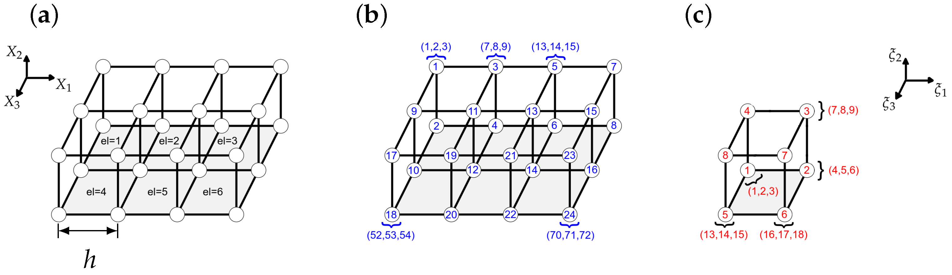
2.2.2. Element ID, Connectivity, and Edof

As in the simplest case, the reference geometry is assumed to be a cuboid to solve Equation (21). This reference cuboid is subdivided into ( n 1 , n 2 , n 3 ) equidistant elements, such that the total number of elements is n el = n 1 n 2 n 3 . The elements are numbered successively along the X 1 , then the X 2 , and lastly the X 3 direction, see Figure 3a.
Each node, which is a corner stone of an element, has three degrees of freedom (dof). Therefore, one element has in total 8 · 3 = 24 dofs and the total number of dofs is n dof = 3 ( n 1 + 1 ) ( n 2 + 1 ) ( n 3 + 1 ) . According to [37], the global node identification is ordered column-wise, with the rule: up-to-bottom, left-to-right, and back-to-front, see Figure 3b. The local node identification of the eight nodes within a single element does not necessarily follow the same convention, and is ordered in counter-clockwise direction instead, see Figure 3c. The global connectivity of each single local element, i.e., the mapping of the blue circled numbers to the red circled numbers, is stored for each element (index “el”) within an array
edof el = [ node 1 x node 1 y node 1 z node 2 x node 8 z ] T N 24
e.g., edof 1 = [ 4 , 5 , 6 , 10 , 11 , 12 , 7 , 8 , 9 , 1 , 2 , 3 , 28 , 29 , 30 , 34 , 35 , 36 , 31 , 32 , 33 , 25 , 26 , 27 ] T . With this at hand, the nodal values of the local displacement vector
u el = u ¯ ( edof el ) R 24 and λ el = λ ¯ ( edof el ) R 24
e . g . , u el = 1 = u ¯ ( edof el = 1 ) = [ u 4 u 5 u 6 u 10 u 26 u 27 ] T
can be extracted for each element from the global displacement vector u ¯ = [ u ¯ 1 u ¯ 2 u ¯ n dof ] . The underbar in the expression ¯ , indicates that a quantity • refers to the ordered nodal values.

2.2.3. Parametric Domain

Now, the solution field inbetween the nodal values must be interpolated. Let a local coordinate vector ξ = ( ξ 1 , ξ 2 , ξ 3 ) T and the parametric domain B ξ = { ξ R 3 | ξ 1 , ξ 2 , ξ 3 [ 1 , 1 ] } be given. As we already performed the mapping from the current to the reference domain, B t B 0 in Equation (10), by using the integration by substitution
B t d v = B 0 J d V
We must map each element to the reference domain B ξ , to perform Gaussian quadrature. In the following case, it is an affine transformation between the reference and the parametric domain,
B 0 d V = el = 1 n el B ξ el J ξ d Ω and J ξ = det X ξ = h 2 3 d V d Ω
where h is the equidistant nodal spacing in the physical domain (see Figure 3a) and 2 is the length of the parametric domain in each direction. Without loss of generality, we set h = 2 in the following.

2.2.4. Ansatz Functions

The ansatz functions for both the displacement and the test function on each element are written in terms of the local coordinate vector ξ , as
u el ( ξ ) = i N i ( ξ ) u el i and λ el ( ξ ) = j N j ( ξ ) λ el j
where it is necessary to note that the entire dependency of u el and λ el on ξ , is carried by the interpolation functions N i only. For computational reasons, often low polynomial degree functions are used, e.g., linear Lagrangian interpolation functions, which read
N i ( ξ ) = 1 2 ( 1 + s 1 i ξ 1 ) 1 2 ( 1 + s 2 i ξ 2 ) 1 2 ( 1 + s 3 i ξ 3 ) where s 1 i = ( 1 ) i s 2 i = sign ( sin ( π 4 ( 1 2 i ) ) s 3 i = sign ( i 4.5 )
and i { 1 , , 8 } . In accordance to the node identification of Section 2.2.2, the sequence of s 1 i is { 1 , 1 , 1 , 1 , 1 , 1 , 1 , 1 } , the sequence of s 2 i is { 1 , 1 , 1 , 1 , 1 , 1 , 1 , 1 } , and the sequence of s 3 i is { 1 , 1 , 1 , 1 , 1 , 1 , 1 , 1 } . In the case of derivatives, one should note that X N i ( X ) = ξ N i ( ξ ) J ξ = ξ N i ( ξ ) 2 h .

2.2.5. Strain–Displacement Matrix

With the ansatz functions at hand, and by using Equation (26), the weak problem (21) reads on each element
B ξ ( ξ N i F el T ) : S el d Ω = B ξ B el T S el V d Ω and S el V = C E el V ( u el )
A quantity called the “non-linear nodal strain–displacement matrix”
B i = F 11 1 N i F 21 1 N i F 31 1 N i F 12 2 N i F 22 2 N i F 32 2 N i F 13 3 N i F 23 3 N i F 33 3 N i F 13 2 N i + F 12 3 N i F 22 3 N i + F 23 2 N i F 32 3 N i + F 33 2 N i F 11 3 N i + F 13 1 N i F 21 3 N i + F 23 1 N i F 33 1 N i + F 31 3 N i F 11 2 N i + F 12 1 N i F 22 1 N i + F 21 2 N i F 31 2 N i + F 32 1 N i
is introduced, where F i j are the entries of the deformation gradient F el , and j ξ j is the derivative in the j th direction. The elemental strain–displacement matrix is composed by the nodal matrices as
B el = [ B i = 1 , , B i = 8 ] R 6 × 24
Alternatively, one can show that the elemental variation in the strain δ E el = B el δ u el relates the non-linear B el -matrix to the variation in the elemental displacements.

2.2.6. Residual of Equilibrium Equation

Now, we can elaborate on the weak form (21) on element basis,
el = 1 n el j = 1 8 λ el j T B ξ B el T S el V d Ω B ξ N j B ˜ el d Ω = el = 1 n el j = 1 8 λ el j T R el = 0
where the term in parentheses is identified as elemental residuum R el , which in turn is given by the difference between internal and external forces on that element,
R el ( u ) = f int f ext R 24
and both, the internal and external elemental forces read
f el int = B ξ B el T S el V d Ω and f el ext = B ξ N j B ˜ el d Ω
Since the nodal values λ i , of the test function are arbitrary, we can find a residual expression
[ λ 1 λ 2 λ n dof ] el = 1 n el j = 1 8 λ el j T λ 1 R el el = 1 n el j = 1 8 λ el j T λ n dof R el = λ ¯ T R ( u ) = 0
Practically, the assembly of the global residual vector R , is given by adding the local values on the corresponding global position as
R ( edof el ) = R ( edof el ) + R el el { 1 , , n el }

2.2.7. Tangential Stiffness Matrix

The tangential stiffness matrix follows from a variation in the residuum,
δ R el ( u ) = B ξ B el T ( δ S el V ) + ( δ B el T ) S el V d Ω = K el δ u el
K el = B ξ B el T C B el + G el T M el G el d Ω R 24 × 24
where G el stores the linear derivatives of the ansatz functions,
G el = [ G k = 1 , , G k = 8 ] R 9 × 24 with G k = 1 N k 1 2 N k 1 3 N k 1 R 9 × 3
and the components of the 1st Piola–Kirchhoff stress tensor S i j are stored in
M el = S 11 1 S 12 1 S 13 1 S 21 1 S 22 1 S 23 1 S 31 1 S 32 1 S 33 1 R 9 × 9
Again, similar to Equation (33), the assembly of the global tangential stiffness matrix reads
K ( edof el , edof el ) = K ( edof el , edof el ) + K el el { 1 , , n el }

2.2.8. Gaussian Quadrature

Equation (38) has polynomial degree d = 3 , so exact integration of some function f, dependent on a polynomial expression of ξ ,
B ξ f ( ξ ) d Ω = gp = 1 n gp f ( ξ gp ) w gp
by summation, is given if the number of Gauss points is n gp = d + 1 2 = 2 , at positions ξ gp = ± 1 3 and weights w gp = 1 .

2.2.9. Newton–Raphson Method

The nodal displacement is found iteratively by using the Newton–Raphson method,
u ¯ i t + 1 = u ¯ i t [ K ( u ¯ i t ) ] 1 R ( u ¯ i t ) = u ¯ it + Δ u ¯ it
where i t is the iteration number. To calculate the displacement update Δ u ¯ it , we use a direct solver until Δ u ¯ it u ¯ it < 0.001 as the termination condition.

2.2.10. Compliance

The compliance of the system is defined in accordance with the strain energy as
c = 1 2 u ¯ T K u ¯ R
with tangential stiffness K , from Equation (41). Sometimes compliance is defined without the factor 1 2  [37]. In terms of an optimization problem, it relates a maximum stiffness demand by means of a minimum compliance.

2.3. Density Based Methods and Filtering Techniques

Although the term density, suggests that the method relies on a quantity extended in space, the density variable x i i { 1 , , n el } , is considered only at the element’s center of mass. It is conceived as an effective quantity during the FEM calculation. The SIMP and BESO methods are based on the formulation that the density interpolates Young’s modulus, see Equation (7). We first review the core idea of the SIMP method, then explain the filtering methods used in the optimization procedure, and show parallels with the BESO method.

2.3.1. SIMP Method

There are many different approaches to keep the binary system, consisting of material and void, from becoming singular in the stiffness tensor, by ascribing either a minimum density x min ,
E i ( x i ) = x i p E 0 x i [ x min , 1 ] i { 1 , , n el }
or a minimum Young’s modulus E min > 0 , to the voids. Within the (modified) SIMP approach the Young’s modulus is given by a convex combination between the solid material ( E 0 ) and the void material ( E min 0 )
E i ( x ˜ ) = E min ( 1 x ˜ i p ) + x ˜ p E 0 x i [ 0 , 1 ] i { 1 , , n el }
which is a function of a (normalized) density x ˜ , with penalization power p > 1 . Here, it is important to distinguish between the (relative) element density x and the filtered (physical) density x ˜ , as described in the following.

2.3.2. Density Filter

According to [44], a basic linear filter density function is defined as
x ˜ i = j w i j x j e . g . , with conical weights w i j = r min dist ( i , j ) j r min dist ( i , j ) , j N i 0 j N i
where the weights should fulfill the partition of unity, j w i j = 1 i , and  r min is an (user) input radius defining the neighborhood N i = ( j : dist ( i , j ) r min ) . In general, the weights influence the resulting structure, and since there is no overall optimum result, they are somehow arbitrary [45]. Other filter types could be defined by Gaussian weights [44], Heaviside filter, dilate and erode filter [46], or filter based on the geometric mean [45]. Nevertheless, what is known for sure, without filtering, the optimum result tends to become a scattered structure, often referred to as a checkerboard, with thin structural parts and/or many tiny holes [45].

2.3.3. Sensitivity Filter

A similar procedure to Equation (47) is applied to the sensitivities, which are the derivatives of the objective function, and reads
c x i ˜ = 1 x i j N i c x j w i j x j i { 1 , , n el }
which is strictly speaking not a density filter because no filtering is conducted regarding the density itself. The sensitivities are used together with the design domain, v ˜ = [ v 1 , , v n ] T and a prescribed volume limit v ¯ , to solve the Karush–Kuhn–Tucker (KKT) condition, which leads to an optimality condition B i = 1 , where
B i = c ( x ˜ ) x i l i v ( x ˜ ) x i 1
should be fulfilled. The value of the Lagrange multiplier l i , satisfying the condition v ( x ˜ ( x n e w ( l i ) ) ) , is the only unknown, and is found by the bisection method. With this, the update reads
x i new = max ( 0 , x i m ) x i B i η max ( 0 , x i m ) min ( 1 , x i + m ) x i B i η min ( 1 , x i m ) x i B i η otherwise
where m is a positive move-limit, and  η is a numerical damping coefficient.

2.3.4. BESO Method

The BESO method relies also on the penalty method of the Young’s modulus, but here, the sensitivity of the objective function is assigned with the total strain energy, α i , of the removed element,
c x i Δ c 1 = α i and α i = 1 2 u i T f i int
Then, the element sensitivity is given by the linear density filter (47), and reads
α ˜ i = w i j α j w i j
To improve the convergence, [32], the sensitivity at the current iteration step (it) is averaged with that from the previous step,
α ˜ j ( it ) α ˜ j ( it ) + α ˜ j ( it - 1 ) 2 , it > 1
Introducing the two threshold constants, α del th for material removal and α add th for material addition, the update reads
x i ( it + 1 ) = x min α i α del th 1 α i > α add th x i ( it ) otherwise
The threshold constants are found by the bisection method. Moreover, the target volume
v ( it ) = max { v ¯ , ( 1 c er v ( it - 1 ) ) }
where c er is the evolutionary ratio determining the percentage of material to be removed. The evolutionary ratio is a number initialized in the previous iteration, and is zero when the target volume is reached. Then, only the topology alters.

2.4. Problem Formulation

Finally, the optimization problem to be solved reads
find x ˜ = [ x 1 , x 2 , . . . , x n el ] T    ( density ) minimize c = 1 2 u ¯ T K u ¯      ( compliance ) subject to v = x ˜ T v ˜ = v ¯    ( volume ) R ( u ¯ ) = f ¯ int f ¯ ext = 0 ¯     ( residuum ) K ( u ¯ ) = δ u ¯ R ( u ¯ ) ( tangential stiffness ) x i { x min , 1 } ( density range )
where in the non-linear case, the displacement u ¯ is found iteratively, by using the Newton–Raphson method. The tilde in the expression ˜ , indicates that a quantity • refers to the ordered elemental values. The optimum structure is found if a termination criterion is fulfilled, e.g., if a certain number of iterations is reached (failure) or the density/compliance difference is marginal between two iteration steps (success), as explained in the following.

2.4.1. Termination Criterion: Density Change

The first termination criterion is density-based, and states that an optimum structure is found if the change between the densities
x ˜ new x ˜ ϵ
according to the L -norm is sufficiently small, ϵ 0.001 . With this at hand, the updated structure would not change in the next iteration step regarding the previous one.

2.4.2. Termination Criterion: Compliance Change

Another termination criterion is based on the change in compliance, defined as a moving average
| i = ( it 9 ) ( it 4 ) c i j = ( it 4 ) ( it ) c j | j = ( it 4 ) ( it ) c j ϵ it > 9
Here, the size of the moving window is somehow arbitrary, and found empirically.

2.5. Chemo-Mechanically Coupled Model

If the optimum structure is found, we need a chemo-mechanically coupled material model to test the particles’ performance. In [47], we formulated a multi-field model for charging and discharging of lithium-ion battery electrodes. Briefly sketched, the model is based on a multiplicative split of the deformation gradient
F = F e F i where F i = J i 2 / 3 1
into an elastic (index e) and purely volumetric inelastic (index i) deformation. The inelastic part should depend on the lithium (Li) concentration c Li , and reads
J i 1 + Ω ¯ ( c Li c 0 )
where Ω ¯ is a normalized partial molar volume and c 0 a reference concentration. With this at hand, the total free energy density of Equation (18) is now, besides the right Cauchy-Green tensor C , dependent on another field variable c Li ,
Ψ = Ψ ela ( C ) + Ψ con ( c Li ) + Ψ int ( c Li )
where Ψ ela ( C ) is the elastic strain energy, e.g.,  Ψ ela ( C ) = Ψ E from (18) but now with concentration dependent elastic moduli, Ψ con ( c Li ) is a double-well potential and Ψ int ( c Li ) accounts for interfacial reactions. Moreover, besides the quasi-static balance of linear momentum, the Cahn–Hilliard equation
c ˙ Li = · ( M δ c Li Ψ )
is an extension of Fickean diffusion, i.e., accounts for the irreversible temporal evolution of the additional concentration field and follows from mass conservation; M , is called a mobility tensor. The Cahn–Hilliard equation is a fourth-order partial differential equation and needs, in the sense of finite element analysis at least, continuous differentiable ansatz functions. Therefore, the obtained optimum structure should be re-meshed by using quadratic B-Splines, and we follow the technique as proposed in [48]. Re-meshing is needed to evaluate the optimum structure in a post-process only, and thus does not affect the mesh during optimization.

3. Results

Here, we first compare the results obtained from linear and non-linear optimization. Then, we elaborate on the force limit, where the results are comparable (within a 3% deviation). With this, we show the simulation results obtained from a single force load. In the next step, we generate structures that result from random force strengths, subject to different constraints on the net force. Finally, all structures’ (normalized) overlays give the most probable shape of a resistant structure to a random contact. This structure is subject to a periodic mechanical motion, and the induced chemo-mechanically coupled change in lithium concentration is studied.

3.1. Reference Parameter Definition

The optimization code listed in Appendix A, relies, according to [32], on the user input ( n x , n y , n z , v ¯ , c er , r min ) and some constants anchored inside the program (see Table 1). If there is no user input, the parameters from the calibration calculation from Section 3.2, are passed automatically. Moreover, the common linear density filter (47) is used in all numerical examples, but can be exchanged by the user if necessary.

3.2. Calibration

For the calibration of the optimization algorithm, we first check that the results obtained from the small strain BESO method are comparable with the small strain SIMP method, in terms of a binarized density at threshold x i = 0.5 i { 1 , , n el } . To this end, we choose the well-known cantilever beam, and set the number of elements to ( 50 , 16 , 4 ) , see Figure 4a. Next, we declare a desired volume of 50% and the normalized force strength to be 10 9 . The convergence plot is shown in Figure 4b and is very similar to the 2D case reported in [32]. The resulting structure from the BESO method is used as input structure for the SIMP optimization calculation, with similar parameters, i.e., we adapted E 0 = 1 , p = 3 , r min = 1.5 , v ¯ = 0.5 , and adjusted E min = 3.1 × 10 2 (see Equations (45) and (46)) and tolx = 0.015 . Since there is almost no difference (two elements change) between the SIMP and the BESO solution at small force strengths, we declare this structure as a reference solution. Then, we increase the force strength and define a deviation D, by element-wise density comparison. Finally, we count only those elements (dark cubes) that do not match the reference solution (see Figure 4c), i.e., the higher D, the more the structure deviates from the reference solution. As expected, the higher the force strength, the higher the deviation.

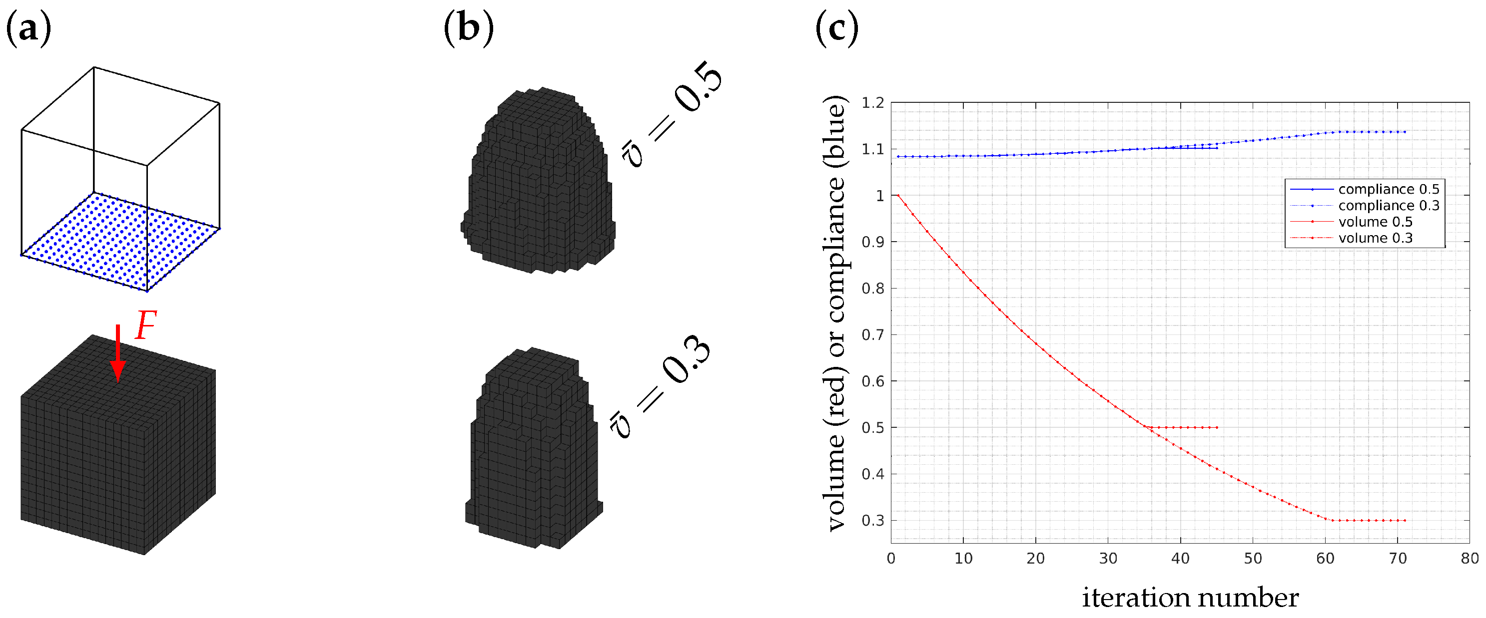
3.3. Central Single Force

Now, the reference geometry is given by a ( 16 , 16 , 16 ) cube, which is subject to a fixture by Dirichlet boundary conditions on the bottom (see blue dots in Figure 5a), a single force acting on top of the surface, and a prescribed volume, of 30% and 50%, respectively. The optimization converges very fast (see Figure 5c) and leads to a conical structure (see Figure 5b), which is almost independent of the force strength applied. Conical structures have already been investigated experimentally in the context of Li-ion battery anodes, by [49], and numerically by [50]. Nevertheless, this kind of structure is resistant to one-sided loadings only, and therefore, we proceed with all-round random contact in the following.

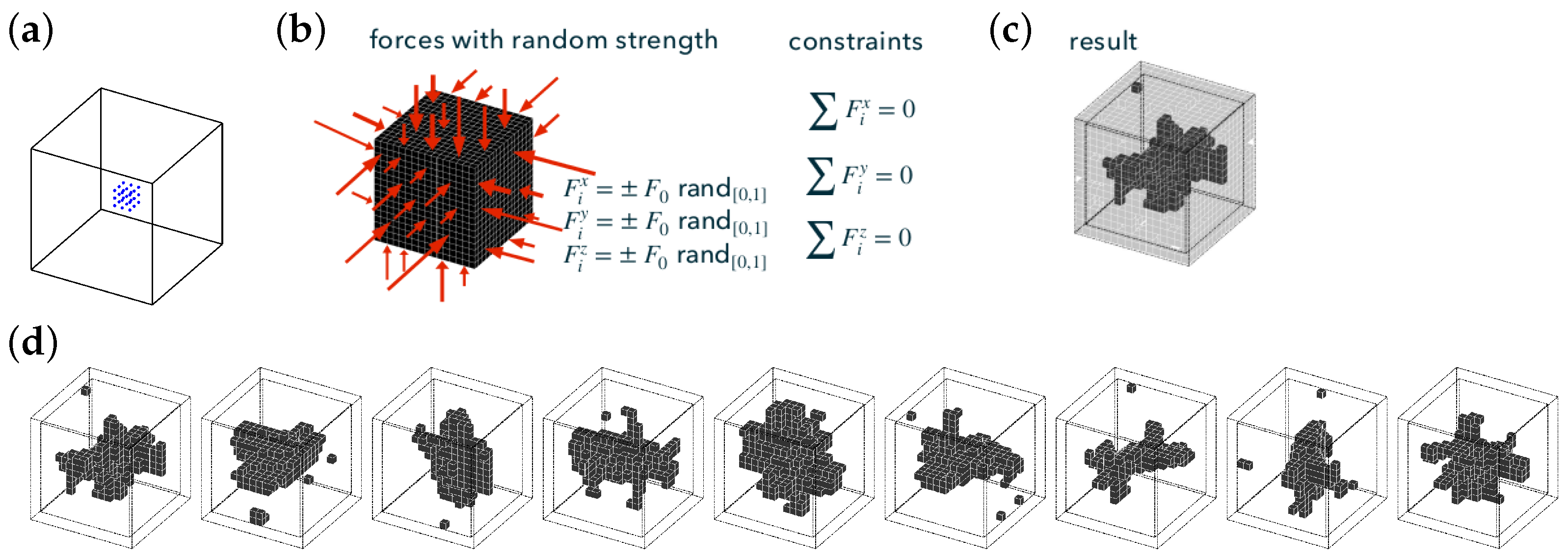
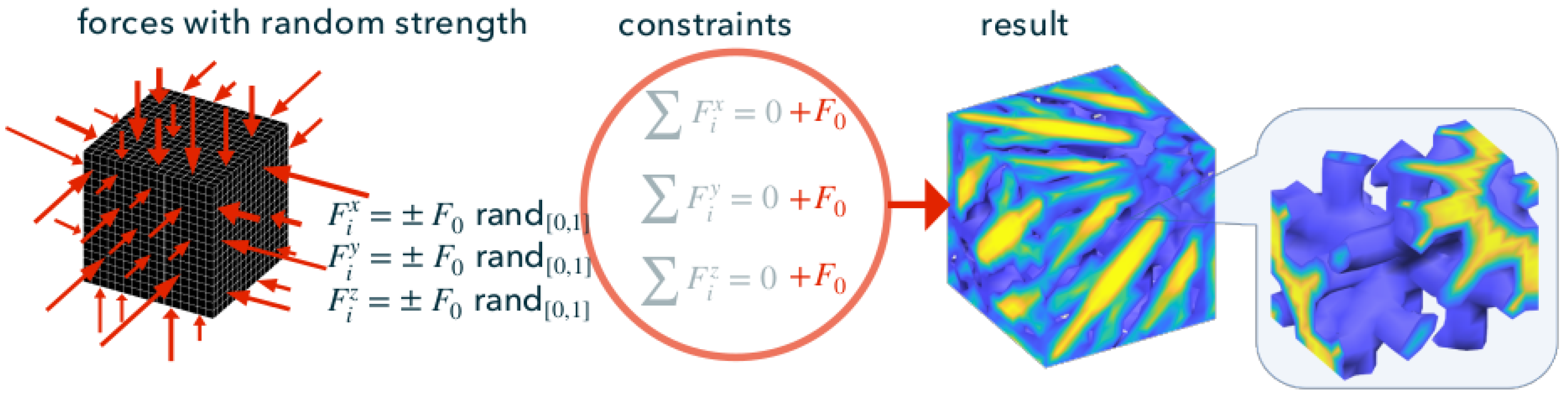
3.4. Forces with Random Strength and Zero Net Strength

Now, we consider again the ( 16 , 16 , 16 ) cube, which is fixed at the center of mass (see blue dots in Figure 6a). We apply forces with random strength, but overall, they are constrained to zero net force (see Figure 6b). Doing so makes the resulting structures look arbitrary (see Figure 6c). The observed island phenomenon is likely due to the applied boundary conditions in the center of the geometry. Due to the randomness of the force strength, the optimum structures are not comparable if repeating the simulation. Especially in Figure 6d, we have omitted the structure’s walls, which were mostly filled with material. Therefore, we must consider a statistical interpretation of the internal structure, as explained in the following subsection.

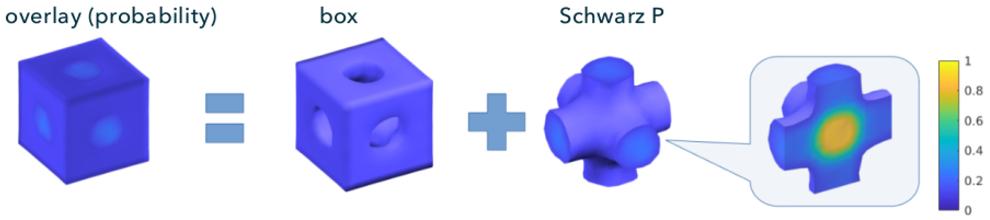
3.5. Probability Density

Since the underlying domain is always kept the same, we can define a probability
P i = s = 1 n sim ( x i ) s n sim i { 1 , , n el }
for each element, which indicates how often the optimized result in the specific domain is provided with material. The cube’s core has the highest probability that it must be filled with solid material, which decreases towards the cube’s corners. Instead of the prescribed volume v ¯ , we can now consult the probability quantile as the superior optimization constraint, which we had to declare for the post-processing. Regarding the color distribution in Figure 7, the most likely structure is a ball (yellow region), very unlikely a fully filled cube (dark blue), and a Schwarz P minimum surface delimits the transition area to an intermediate structure. The Schwarz P surface itself can be described analytically by the function
cos ( X 1 ) + cos ( X 2 ) + cos ( X 3 ) = 0
In the following, we will mesh it as a solid and expose it to chemo-mechanical cycling.

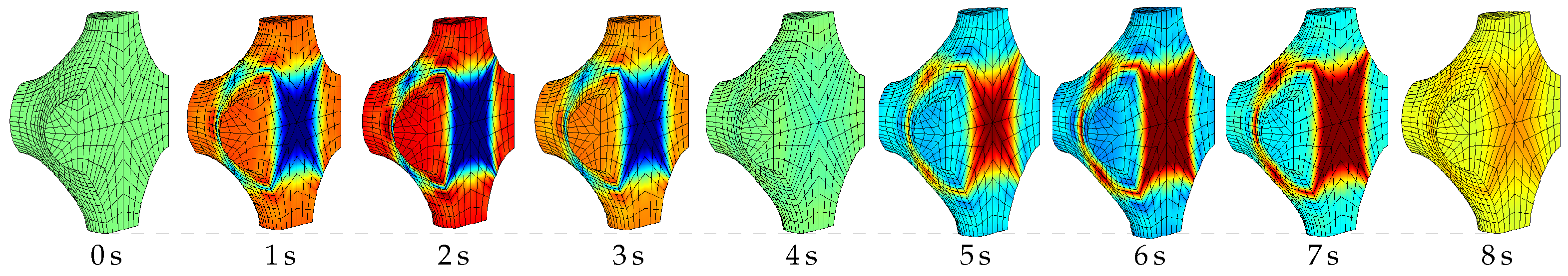
3.6. Periodic Loading of Schwarz P Structure

The topology-optimized structure is now subjected to sinusoidal cyclic loading, and an initial value problem is solved using the chemo-mechanically coupled model. In Figure 8, the concentration distribution is shown, where the concentration is pushed outward in a compressive motion and vice versa. Since the constitutive law follows the thermodynamics of irreversible processes, it can be seen that after the first mechanical cycle, the concentration distribution does not return to the uniformly distributed original state, but an induced pattern persists.

3.7. Forces with Random Strength and Non-Zero Net Strength

Previously we assumed the constraint of a vanishing total force. Now, a net force on the object is prescribed, and then, the optimum topology changes to an eighth of a bee-shaped structure, with spikes in the diagonal corners, see Figure 9.

4. Discussion

The core question of this paper, was related to the optimal geometry of a silicon anode exposed to a random contact. It is known that silicon anodes swell to multiples of their original volume. Thus, depending on the charging behavior, the interaction between the particles is somewhat random, regarding the force strength and the local position of the occurrence. We have developed and provided a compact Matlab code to address the question of an optimal geometry that is as resistant as possible to this type of force action. The code is based on the two papers by [32,37]. The published code of the first reference is known for its particular simplicity of implementation of boundary conditions, and the second reference for its fast convergence rate, whereas the latter code had been published only in 2D. In addition, all studies we have performed using the new code, provide symmetric structures under symmetric loading, which is infrequent in the literature. Then, we subjected a cube to random loading but obtained structures challenging to interpret. However, we considered the normalized overlap as the probability density when overlapping the structures resulting from many simulations. As a result, we obtained the symmetric Schwarz P structure at a specific threshold, which has a minimum surface property. Such results sound promising in the context of electrodes, where structures with minimum surface area are desired. Furthermore, this method also yields what one would intuitively expect, e.g., a structure concentrated along the diagonal in the case of diagonal loading. Finally, the material model is chosen, so that it can be extended in the future by a crack density field, for a crack propagation study.

5. Conclusions

Here, we elaborated on large, geometrically non-linear deformations of battery anodes, intending to find an optimum (maximum stiff) electrode design when subject to random contact, in terms of random forces. The optimization technique relies on the BESO method, where the solution procedure includes non-linear finite element analysis, specific sensitivity filtering, and an improved weighting of the historical information, to ensure fast convergence. The existing 2D Matlab code reported in [32] was extended here to 3D, attached in the appendix, and applied to several design problems. Even at moderate volume fractions, the resulting topologies are hard to compare with each other. Thus, in such cases, the optimum structures are found by performing multiple simulations and interpreting their (normalized) overlap as a probability density.

Author Contributions

Conceptualization, M.W. and S.B.; methodology, M.W. and K.W.; software, M.W.; validation, S.B. and K.W.; formal analysis, M.W. and K.W.; investigation, S.B. and M.W.; resources, M.W.; writing—original draft preparation, M.W.; writing—review and editing, S.B. and K.W.; visualization, M.W. and S.B.; supervision, K.W.; project administration, K.W.; funding acquisition, K.W. All authors have read and agreed to the published version of the manuscript.

Funding

This research was funded by DFG grant number 2525/11-1.

Institutional Review Board Statement

Not applicable.

Informed Consent Statement

Not applicable.

Data Availability Statement

Data can be reproduced by using the Matlab code from Appendix A.

Conflicts of Interest

The authors declare no conflict of interest.

Abbreviations

    The following abbreviations are used in this manuscript:
BESOBi-evolutionary structural optimization
dofDegree of freedom
ESOEvolutionary structural optimization
FEMFinite element method
LiLithium
SiSilicon
SIMPSolid isotropic material with penalization

List of Symbols

The following symbols are used in this manuscript:
el • With respect to element n , N Normal vector
it • With respect to iteration numberpPenalization power
T Transpose of •PProbability density
V Voigt notation of • P 1st Piola–Kirchhoff stress tensor
¯ Prescribed quantity r min Filter radius
¯ Arranged with respect to nodal values R Residual vector
˜ Arranged with respect to elemental values S 2nd Piola–Kirchhoff stress tensor
tr ( ) Sum of diagonal elements (trace)ttime
t , T Cauchy traction vector
0 Zero matrix u , U Displacement vector
1 Identity matrix v , V Volume
v Design domain
a , A AreawWeights
B i Optimality condition x , x min Density variable, minimum density
b , B ˜ Body force density x ˜ Filtered density
B Strain–displacement matrix x , X Point of a continuum
cCompliance
c 0 Ref Lithium ion concentration α i Total strain energy of removed element
c er Evolutionary ratio α th Threshold constant
c Li Lithium ion concentration δ Variational derivative
C Right Cauchy–Green strain tensor ϵ Small number 1
dPolynomial degree ε Small strain tensor
DDeviation η Damping coefficient
edof el edof array for a specific element λ , μ Lamé parameter
EYoung’s modulus λ Test function
E n Total strain energy of removed element ν Poisson number
E Green–Lagrangian strain tensor ξ Local coordinate vector
F 0 Force strength σ Cauchy stress tensor
f Force Ψ Strain energy density function
F Deformation gradient Ω Volume (parametric domain)
G el Linear derivatives matrix Ω ¯ Normalized partial molar volume
hEquidistant nodal spacing
JJacobian B Body (0 reference, t actual, ξ parametric)
K Stiffness matrix B Boundary of body
lLagrange multiplier C Elasticity tensor
mMove limit M Mobility tensor
M el Stress components matrix N Neighborhood
n el Number of elements
n gp Number of Gauss points , Partial derivative
n sim Number of simulationsEmpty set
N i Interpolation function , Union and intersection of sets

Appendix A. Matlab Code

In Listing A1, we show the condensed 3D Matlab source code with sufficient comments. Of course, this code can be accelerated at the expense of readability.
Listing A1.
3D Matlab source code for non-linear topology optimization based on the BESO method.
1
function [x,U]=TopOptBesoNL3D_mdpi(nelx,nely,nelz,volfrac,er,rmin)
2
%-- if no input, then use some default values:
3
if nargin<6; nelx=50; nely=16; nelz=4; volfrac=0.5; er=0.02; rmin=1.5; end
4
%-- force strength (F0)
5
F0=1e-9; E=1; nu=0.3; xmin=3e-5; penal=1; tolx=0.0001; maxloop=500;
6
vol=1; loop=0; change=1; pos=1;
7
x=ones(nely,nelx,nelz); c=zeros(1,maxloop);
8
nele=nelx*nely*nelz; ndof=3*(nelx+1)*(nely+1)*(nelz+1);
9
%-- loads, here: at right end along z-direction
10
[il,jl,kl] = meshgrid(nelx, 0, 0:nelz);
11
loadnid=kl*(nelx+1)*(nely+1)+il*(nely+1)+(nely+1-jl);
12
loaddof=3*loadnid(:)-1;
13
F=sparse(loaddof,1,F0,ndof,1);
14
%-- supports, here: at left end along y- and z-direction
15
[iif,jf,kf]=meshgrid(0,0:nely,0:nelz);
16
fixednid=kf*(nelx+1)*(nely+1)+iif*(nely+1)+(nely+1-jf);
17
fixeddof=[3*fixednid(:); 3*fixednid(:)-1; 3*fixednid(:)-2];
18
%-- get free dofs
19
freedofs=setdiff(1:ndof,fixeddof);
20
%-- edof
21
edofMat=zeros(nele,24); ID=reshape(1:ndof/3,nely+1,nelx+1,nelz+1);
22
for iz=1:nelz
23
for ix=1:nelx
24
for iy=1:nely
25
    edofMat_1=ID([0,1]+iy,[0,1]+ix,[0,1]+iz);
26
    edofMat_1=edofMat_1([2,4,3,1,6,8,7,5]);
27
    edofMat_1=3*(edofMat_1(:)-1)’ + (1:3)’;
28
    edofMat(pos,:)=edofMat_1(:)’;
29
    pos=pos+1;
30
end
31
end
32
end
33
%-- START WITH ITERATION
34
while change>tolx && loop<maxloop
35
loop=loop+1;
36
if loop>1; olddc=dc; vol=max(vol*(1-er),volfrac); end
37
%-- displacement (U), sensitivities (dc) and compliance (c) from FEA
38
[U,dc,c(loop)]=FEA(nele,ndof,edofMat,x,penal,E,nu,F,freedofs);
39
%-- filtering of sensivities
40
dc=reshape(dc,nely,nelx,nelz); dc=check(nelx,nely,nelz,rmin,dc);
41
%-- stabilization of evolutionary process
42
if loop>1; dc=(dc+olddc)/2; end
43
%-- BESO design update
44
if loop>1; x=ADDDEL(nele,vol,dc,x,xmin); end
45
%-- convergence factor (change)
46
if loop>10; change=abs(sum(c(loop-9:loop-5))-sum(c(loop-4:loop)))/sum(c(loop-4:loop)); end
47
%-- print results
48
fprintf(’It.:%4i Obj.:%10.4f Vol.:%6.3f ch.:%6.3f\n’,loop,c(loop)*1e15,sum(x(:))/nele,change);
49
%-- plot densities
50
display_3D(x);
51
end
52
end
53
%-- BESO design update
54
function [x]=ADDDEL(nele,volfrac,dc,x,xmin)
55
l1=min(dc(:)); l2=max(dc(:));
56
while abs((l2-l1)/l2)>1e-5; th=(l1+l2)/2; x=max(xmin,sign(dc-th));
57
if sum(x(:))>volfrac*nele; l1=th; else; l2=th; end
58
end
59
end
60
%-- linear density filter
61
function [dcf]=check(nelx,nely,nelz,rmin,dc)
62
dcf=zeros(nely,nelx,nelz);
63
for k1=1:nelz
64
for i=1:nelx
65
for j=1:nely
66
zum=0;
67
for k2=max(k1-floor(rmin),1):min(k1+floor(rmin),nelz)
68
for k=max(i-floor(rmin),1):min(i+floor(rmin),nelx)
69
for l=max(j-floor(rmin),1):min(j+floor(rmin),nely)
70
    fac=rmin-sqrt((i-k)^2+(j-l)^2+(k1-k2)^2);
71
    zum=zum+max(0,fac);
72
    dcf(j,i,k1)=dcf(j,i,k1)+max(0,fac)*dc(l,k,k2);
73
end
74
end
75
end
76
dcf(j,i,k1)=dcf(j,i,k1)/zum;
77
end
78
end
79
end
80
end
81
%-- FEA
82
function [U,dc,cloop]=FEA(nele,ndof,edofMat,x,penal,E,nu,F,freedofs)
83
%-- initialization of global stiffness matrix (K), residuum (R) and displacement (U)
84
K=sparse(ndof,ndof); R=zeros(ndof,1); dU=R; U=R; dc=zeros(nele,1); del=1; loop=0;
85
%-- Iteratively solve the geometric nonlinear FE balance equation
86
while del>0.001 && loop<4 % or increase for more iterations
87
cloop=0; loop=loop+1;
88
%-- loop over elements
89
for ele=1:nele
90
%-- elemental quantities
91
xe=x(ele); edof=edofMat(ele,:)’; Ue=U(edof);
92
[RE,KE,dce]=solver(E,nu,Ue,xe,penal);
93
%-- assembly
94
K(edof,edof)=K(edof,edof)+KE; R(edof)=R(edof)+RE; dc(ele)=dce;
95
cloop=cloop+0.5*xe^penal*Ue’*KE*Ue;
96
end
97
%-- residual, tangent and displacement
98
R=sparse(R+F); K=sparse((K+K’)/2);
99
%-- direct solver
100
dU(freedofs,:)=K(freedofs,freedofs)\R(freedofs,:); U=U+dU; del=norm(dU,2)/norm(U,2);
101
end
102
end
103
%-- FE solver
104
function [RE,KE,dc]=solver(E,nu,Ue,xele,penal)
105
%-- initialization
106
RE=zeros(24,1); KE=zeros(24,24); dc=0; sq=1/sqrt(3); Y=eye(3); Z=zeros(3);
107
%-- displacements (uij) where i=number, j=direction
108
u11=Ue(1); u21=Ue(4); u31=Ue(7); u41=Ue(10); u51=Ue(13); u61=Ue(16); u71=Ue(19); u81=Ue(22);
109
u12=Ue(2); u22=Ue(5); u32=Ue(8); u42=Ue(11); u52=Ue(14); u62=Ue(17); u72=Ue(20); u82=Ue(23);
110
u13=Ue(3); u23=Ue(6); u33=Ue(9); u43=Ue(12); u53=Ue(15); u63=Ue(18); u73=Ue(21); u83=Ue(24);
111
%-- elasticity tensor (C)
112
C=xele^penal*E/((1+nu)*(1-2*nu))*[(1-2*nu)*Y+nu*(Z+1),Z;Z,(0.5-nu)*Y];
113
%-- Gaussian quadrature over 3^2=8 points and weights=1
114
for gp=1:8
115
%--sign (si) of ansatz functions
116
s1=1-2*mod(gp,2); s2=sign(sin(pi/4*(1-2*gp))); s3=sign(gp-4.5);
117
p1=1+s1*sq; m1=1-s1*sq; p2=1+s2*sq; m2=1-s2*sq; p3=1+s3*sq; m3=1-s3*sq;
118
%-- derivative of ansatz functions Ni wrt j, (dNij) where e.g. dN21=-dN11
119
dN11=-m2*m3/8;dN31= p2*m3/8;dN51=-m2*p3/8;dN71= p2*p3/8;
120
dN12=-m1*m3/8;dN22=-p1*m3/8;dN52=-m1*p3/8;dN62=-p1*p3/8;
121
dN13=-m1*m2/8;dN23=-p1*m1/8;dN33=-p1*p2/8;dN43=-m1*p2/8;
122
dN1=[dN11,-dN11,dN31,-dN31,dN51,-dN51,dN71,-dN71];
123
dN2=[dN12,dN22,-dN22,-dN12,dN52,dN62,-dN62,-dN52];
124
dN3=[dN13,dN23,dN33,dN43,-dN13,-dN23,-dN33,-dN43];
125
%-- components of deformation gradient (Fij)
126
F11=dN11*(u11-u21)+dN31*(u31-u41)+dN51*(u51-u61)+dN71*(u71-u81)+1;
127
F12=dN11*(u12-u22)+dN31*(u32-u42)+dN51*(u52-u62)+dN71*(u72-u82);
128
F13=dN11*(u13-u23)+dN31*(u33-u43)+dN51*(u53-u63)+dN71*(u73-u83);
129
F21=dN12*(u11-u41)+dN22*(u21-u31)+dN52*(u51-u81)+dN62*(u61-u71);
130
F22=dN12*(u12-u42)+dN22*(u22-u32)+dN52*(u52-u82)+dN62*(u62-u72)+1;
131
F23=dN12*(u13-u43)+dN22*(u23-u33)+dN52*(u53-u83)+dN62*(u63-u73);
132
F31=dN13*(u11-u51)+dN23*(u21-u61)+dN33*(u31-u71)+dN43*(u41-u81);
133
F32=dN13*(u12-u52)+dN23*(u22-u62)+dN33*(u32-u72)+dN43*(u42-u82);
134
F33=dN13*(u13-u53)+dN23*(u23-u63)+dN33*(u33-u73)+dN43*(u43-u83)+1;
135
F1=[F11,F21,F31]; F2=[F12,F22,F32]; F3=[F13,F23,F33];
136
%-- strain-displacement matrix (B)
137
B1=repmat([F1;F2;F3],1,8).*reshape(repmat([dN1;dN2;dN3],3,1),3,24);
138
B2=repmat([F3;F1;F2],1,8).*reshape(repmat([dN2;dN3;dN1],3,1),3,24);
139
B3=repmat([F2;F3;F1],1,8).*reshape(repmat([dN3;dN1;dN2],3,1),3,24);
140
B=[B1;B2+B3]; BT=B’; CB=C*B; SV=CB*Ue;
141
%-- elemental residuum (RE), stiffness matrix (KE), and compliance (dc) update
142
Fint=BT*SV; RE=RE-Fint; dc=dc+0.5*Ue’*Fint;
143
G=[dN11*Y,-dN11*Y,dN31*Y,-dN31*Y,dN51*Y,-dN51*Y,dN71*Y,-dN71*Y;
144
   dN12*Y,dN22*Y,-dN22*Y,-dN12*Y,dN52*Y,dN62*Y,-dN62*Y,-dN52*Y;
145
   dN13*Y,dN23*Y,dN33*Y,dN43*Y,-dN13*Y,-dN23*Y,-dN33*Y,-dN43*Y];
146
M=[SV(1)*Y,SV(6)*Y,SV(5)*Y;SV(6)*Y,SV(2)*Y,SV(4)*Y;SV(5)*Y,SV(4)*Y,SV(3)*Y];
147
KE=KE+BT*CB+G’*M*G;
148
end
149
end
150
%--display
151
function display_3D(rho)
152
[nely,nelx,nelz]=size(rho); cla; face = [1 2 3 4; 2 6 7 3; 4 3 7 8; 1 5 8 4; 1 2 6 5; 5 6 7 8];
153
for z=0:(nelz-1)
154
for x=0:(nelx-1)
155
for y=nely:-1:1
156
R = rho(1+nely-y,x+1,z+1);
157
if R>0.5
158
    vert=[x,-z,y;x,-z,y-1;x+1,-z,y-1;x+1,-z,y;x,-z-1,y;x,-z-1,y-1;x+1,-z-1,y-1;x+1,-z-1,y];
159
    patch(’Faces’,face,’Vertices’,vert,’FaceColor’,(0.2+0.8*(1-R))*[1,1,1]); hold on;
160
end
161
end
162
end
163
end
164
axis equal; axis tight; axis off; box onview([30,30]); pause(1e-9);
165
end
166
%-- Disclaimer:
167
%-- The authors reserves all rights for the program.
168
%-- The code may be distributed and used for educational purposes.
169
%-- The authors do not guarantee that the code is free from errors, and
170
%-- they shall not be liable in any event caused by the use of the code.
171
%-- contact: marek.werner@uni-siegen.de

References

  1. Schmit, L.A. Structural design by systematic synthesis. In Proceedings of the 2nd Conference on Electronic Computation, Pittsburgh, PA, USA, 8–10 September 1960; ASCE: New York, NY, USA, 1960; pp. 105–132. [Google Scholar]
  2. Bendsøe, M.P.; Kikuchi, N. Generating optimal topologies in structural design using a homogenization method. Comput. Methods Appl. Mech. Eng. 1988, 71, 197–224. [Google Scholar] [CrossRef]
  3. Ballo, F.M.; Gobbi, M.; Mastinu, G.; Previati, G. Optimal Lightweight Construction Principles, 1st ed.; Springer: Cham, Switzerland, 2021. [Google Scholar] [CrossRef]
  4. Czerwinski, F. Current Trends in Automotive Lightweighting Strategies and Materials. Materials 2021, 14, 6631. [Google Scholar] [CrossRef] [PubMed]
  5. Chen, L.; Zhang, Y.; Chen, Z.; Xu, J.; Wu, J. Topology optimization in lightweight design of a 3D-printed flapping-wing micro aerial vehicle. Chin. J. Aeronaut. 2020, 33, 3206–3219. [Google Scholar] [CrossRef]
  6. Orme, M.; Madera, I.; Gschweitl, M.; Ferrari, M. Topology Optimization for Additive Manufacturing as an Enabler for Light Weight Flight Hardware. Designs 2018, 2, 51. [Google Scholar] [CrossRef] [Green Version]
  7. Liu, S.; Hu, R.; Li, Q.; Zhou, P.; Dong, Z.; Kang, R. Topology optimization-based lightweight primary mirror design of a large-aperture space telescope. Appl. Opt. 2014, 53, 8318–8325. [Google Scholar] [CrossRef]
  8. Zhu, J.; Zhou, H.; Wang, C.; Zhou, L.; Yuan, S.; Zhang, W. A review of topology optimization for additive manufacturing: Status and challenges. Chin. J. Aeronaut. 2021, 34, 91–110. [Google Scholar] [CrossRef]
  9. Ismail, A.Y.; Na, G.; Koo, B. Topology and Response Surface Optimization of a Bicycle Crank Arm with Multiple Load Cases. Appl. Sci. 2020, 10, 2201. [Google Scholar] [CrossRef] [Green Version]
  10. Matsimbi, M.; Nziu, P.K.; Masu, L.M.; Maringa, M. Topology Optimization of Automotive Body Structures: A review. Int. J. Eng. Res. Technol. 2021, 13, 4282–4296. [Google Scholar]
  11. Omar, M.A. Chain Drive Simulation Using Spatial Multibody Dynamics. Adv. Mech. Eng. 2014, 6, 378030. [Google Scholar] [CrossRef] [Green Version]
  12. Jiang, Y.; Zhan, K.; Xia, J.; Zhao, M. Topology Optimization for Minimum Compliance with Material Volume and Buckling Constraints under Design-Dependent Loads. Appl. Sci. 2023, 13, 646. [Google Scholar] [CrossRef]
  13. Kang, Z.; Liu, P.; Li, M. Topology optimization considering fracture mechanics behaviors at specified locations. Struct. Multidiscip. Optim. 2017, 55, 1847–1864. [Google Scholar] [CrossRef]
  14. Li, D.; Kim, I.Y. Multi-material topology optimization for practical lightweight design. Struct. Multidiscip. Optim. 2018, 58, 1081–1094. [Google Scholar] [CrossRef]
  15. Rieser, J.; Zimmermann, M. Topology optimization of periodically arranged components using shared design domains. Struct. Multidiscip. Optim. 2021, 65, 18. [Google Scholar] [CrossRef]
  16. Vatanabe, S.L.; Lippi, T.N.; de Lima, C.R.; Paulino, G.H.; Silva, E.C. Topology optimization with manufacturing constraints: A unified projection-based approach. Adv. Eng. Softw. 2016, 100, 97–112. [Google Scholar] [CrossRef] [Green Version]
  17. Zhang, L.; Al-Mamun, M.; Wang, L.; Dou, Y.; Qu, L.; Dou, S.X.; Liu, H.K.; Zhao, H. The typical structural evolution of silicon anode. Cell Rep. Phys. Sci. 2022, 3, 100811. [Google Scholar] [CrossRef]
  18. Roy, T.; Salazar de Troya, M.A.; Worsley, M.A.; Beck, V.A. Topology optimization for the design of porous electrodes. Struct. Multidiscip. Optim. 2022, 65, 171. [Google Scholar] [CrossRef]
  19. Mitchell, S.L. Topology Optimization of Silicon Anode Structures for Lithium-Ion Battery Applications; California Institute of Technology: Pasadena, CA, USA, 2016. [Google Scholar] [CrossRef]
  20. Bai, X.; Zhang, H.; Lin, J. A three-dimensionally hierarchical interconnected silicon-based composite for long-cycle-life anodes towards advanced Li-ion batteries. J. Alloys Compd. 2022, 925, 166563. [Google Scholar] [CrossRef]
  21. Teki, R.; Datta, M.K.; Krishnan, R.; Parker, T.C.; Lu, T.M.; Kumta, P.N.; Koratkar, N. Nanostructured Silicon Anodes for Lithium Ion Rechargeable Batteries. Small 2009, 5, 2236–2242. [Google Scholar] [CrossRef]
  22. Liang, B.; Liu, Y.; Xu, Y. Silicon-based materials as high capacity anodes for next generation lithium ion batteries. J. Power Sources 2014, 267, 469–490. [Google Scholar] [CrossRef]
  23. Bluhm, G.L.; Sigmund, O.; Poulios, K. Internal contact modeling for finite strain topology optimization. Comput. Mech. 2021, 67, 1099–1114. [Google Scholar] [CrossRef]
  24. Wu, Y.; Guo, Z.S. Concentration Distribution and Stresses in Porous Electrodes with Particle-Particle Contact. J. Electrochem. Soc. 2021, 168, 090507. [Google Scholar] [CrossRef]
  25. Kristiansen, H.; Poulios, K.; Aage, N. Topology optimization for compliance and contact pressure distribution in structural problems with friction. Comput. Methods Appl. Mech. Eng. 2020, 364, 112915. [Google Scholar] [CrossRef]
  26. Niu, C.; Zhang, W.; Gao, T. Topology optimization of elastic contact problems with friction using efficient adjoint sensitivity analysis with load increment reduction. Comput. Struct. 2020, 238, 106296. [Google Scholar] [CrossRef]
  27. Lu, B.; Zhao, Y.; Feng, J.; Song, Y.; Zhang, J. Mechanical contact in composite electrodes of lithium-ion batteries. J. Power Sources 2019, 440, 227115. [Google Scholar] [CrossRef]
  28. Sigmund, O. A 99 line topology optimization code written in Matlab. Struct. Multidiscip. Optim. 2001, 21, 120–127. [Google Scholar] [CrossRef]
  29. Da, D.; Xia, L.; Li, G.; Huang, X. Evolutionary topology optimization of continuum structures with smooth boundary representation. Struct. Multidiscip. Optim. 2018, 57, 2143–2159. [Google Scholar] [CrossRef]
  30. Fu, Y.F.; Rolfe, B.; Chiu, L.; Wang, Y.; Huang, X.; Ghabraie, K. SEMDOT: Smooth-edged material distribution for optimizing topology algorithm. Adv. Eng. Softw. 2020, 150, 102921. [Google Scholar] [CrossRef]
  31. Huang, X.; Li, W. Three-field floating projection topology optimization of continuum structures. Comput. Methods Appl. Mech. Eng. 2022, 399, 115444. [Google Scholar] [CrossRef]
  32. Han, Y.; Xu, B.; Liu, Y. An efficient 137-line MATLAB code for geometrically nonlinear topology optimization using bi-directional evolutionary structural optimization method. Struct. Multidiscip. Optim. 2021, 63, 2571–2588. [Google Scholar] [CrossRef]
  33. Zhu, B.; Zhang, X.; Zhang, H.; Liang, J.; Zang, H.; Li, H.; Wang, R. Design of compliant mechanisms using continuum topology optimization: A review. Mech. Mach. Theory 2020, 143, 103622. [Google Scholar] [CrossRef]
  34. Buhl, T.; Pedersen, C.B.W.; Sigmund, O. Stiffness design of geometrically nonlinear structures using topology optimization. Struct. Multidiscip. Optim. 2000, 19, 93–104. [Google Scholar] [CrossRef]
  35. Wang, F.; Lazarov, B.S.; Sigmund, O.; Jensen, J.S. Interpolation scheme for fictitious domain techniques and topology optimization of finite strain elastic problems. Comput. Methods Appl. Mech. Eng. 2014, 276, 453–472. [Google Scholar] [CrossRef]
  36. Xue, R.; Liu, C.; Zhang, W.; Zhu, Y.; Tang, S.; Du, Z.; Guo, X. Explicit structural topology optimization under finite deformation via Moving Morphable Void (MMV) approach. Comput. Methods Appl. Mech. Eng. 2019, 344, 798–818. [Google Scholar] [CrossRef]
  37. Liu, K.; Tovar, A. An efficient 3D topology optimization code written in Matlab. Struct. Multidiscip. Optim. 2014, 50, 1175–1196. [Google Scholar] [CrossRef] [Green Version]
  38. Holzapfel, G. Nonlinear Solid Mechanics: A Continuum Approach for Engineering; Wiley: Hoboken, NJ, USA, 2000. [Google Scholar] [CrossRef]
  39. de Borst, R.; Crisfield, M.A.; Remmers, J.J.C.; Verhoosel, C.V. Non-linear Finite Element Analysis. In Non-Linear Finite Element Analysis of Solids and Structures; John Wiley & Sons, Ltd.: Hoboken, NJ, USA, 2012; Chapter 2; pp. 31–62. [Google Scholar] [CrossRef] [Green Version]
  40. Sautter, K.B.; Meßmer, M.; Teschemacher, T.; Bletzinger, K.U. Limitations of the St. Venant–Kirchhoff material model in large strain regimes. Int. J. Non-Linear Mech. 2022, 147, 104207. [Google Scholar] [CrossRef]
  41. Ogden, R.W.; Hill, R. Large deformation isotropic elasticity – on the correlation of theory and experiment for incompressible rubberlike solids. Proc. R. Soc. Lond. A. Math. Phys. Sci. 1972, 326, 565–584. [Google Scholar] [CrossRef]
  42. Miehe, C. Aspects of the formulation and finite element implementation of large strain isotropic elasticity. Int. J. Numer. Methods Eng. 1994, 37, 1981–2004. [Google Scholar] [CrossRef]
  43. Hartmann, S. The Class of Simo & Pister-Type Hyperelasticity Relations; Technical Report Series; Clausthal University of Technology: Clausthal-Zellerfeld, Germany, 2010. [Google Scholar]
  44. Bruns, T.E.; Tortorelli, D.A. Topology optimization of non-linear elastic structures and compliant mechanisms. Comput. Methods Appl. Mech. Eng. 2001, 190, 3443–3459. [Google Scholar] [CrossRef]
  45. Svanberg, K.; Svärd, H. Density filters for topology optimization based on the Pythagorean means. Struct. Multidiscip. Optim. 2013, 48, 859–875. [Google Scholar] [CrossRef]
  46. Sigmund, O. Morphology-based black and white filters for topology optimization. Struct. Multidiscip. Optim. 2007, 33, 401–424. [Google Scholar] [CrossRef] [Green Version]
  47. Werner, M.; Pandolfi, A.; Weinberg, K. A multi-field model for charging and discharging of lithium-ion battery electrodes. Contin. Mech. Thermodyn. 2021, 33, 661–685. [Google Scholar] [CrossRef]
  48. Werner, M.; Weinberg, K. B-Spline meshing for high-order finite element analyses of multi-physics problems. Tech.-Mech.-Eur. J. Eng. Mech. 2021, 41, 1–11. [Google Scholar] [CrossRef]
  49. Berla, L.A.; Lee, S.W.; Ryu, I.; Cui, Y.; Nix, W.D. Robustness of amorphous silicon during the initial lithiation/delithiation cycle. J. Power Sources 2014, 258, 253–259. [Google Scholar] [CrossRef]
  50. Werner, M.; Weinberg, K. Towards structural optimization of lithium battery anodes. PAMM 2018, 18, e201800227. [Google Scholar] [CrossRef]
Figure 1. Optimizing a plate subjected to opposite forces at both ends leads to a bicycle chain link. In (a), the initial volume is shown, (b) shows the optimum material distribution, and (c) is the technical application.
Solids 04 00007 g001
Figure 2. Sketch of silicon particle contact during lithiation. The initially cylindrical rods swell over time to balloon-shaped objects, and might touch each other.
Solids 04 00007 g002
Figure 3. (a) Element ID, (b) global connectivity, and (c) local connectivity.
Solids 04 00007 g003
Figure 4. Optimization of a cantilever beam: (a) boundary conditions and reference optimum design, (b) evolutionary histories of the volume fraction and the compliance ( × 10 15 ), and (c) deviation from reference solution dependent on the force strength.
Solids 04 00007 g004
Figure 5. Optimization of a cube subjected to a single force: (a) boundary conditions, (b) optimum structures at prescribed volumes, and (c) evolutionary histories of the volume fraction and the compliance ( × 10 18 ).
Solids 04 00007 g005
Figure 6. Optimization of a cube: (a) boundary conditions for the fixture, (b) random strength, as boundary condition, with a zero net force constraint, (c) optimum structure, and (d) more optimum structures showing different pattern.
Solids 04 00007 g006
Figure 7. Color code overlay of optimization results and their decomposition into a box and a Schwarz P structure (for P > 0.1 ).
Solids 04 00007 g007
Figure 8. Concentration distribution due to compression/tension, dashed line serves for guidance.
Solids 04 00007 g008
Figure 9. Optimization of a cube, subject to forces with random strength and a net force constraint.
Solids 04 00007 g009
Table 1. Variables (top row), their designation inside the Matlab code (middle row), and their reference values (bottom row).
E ν x min p v ¯ r min c er F 0 ϵ
EnuxminpenalvolfracrminerF0tolx
10.3 3 × 10 5 10.51.50.02 10 9 10 4
Disclaimer/Publisher’s Note: The statements, opinions and data contained in all publications are solely those of the individual author(s) and contributor(s) and not of MDPI and/or the editor(s). MDPI and/or the editor(s) disclaim responsibility for any injury to people or property resulting from any ideas, methods, instructions or products referred to in the content.

