
A Comprehensive Study on the Styrene–GTR Radical Graft Polymerization: Combination of an Experimental Approach, on Different Scales, with Machine Learning Modeling

Abstract
:1. Introduction
2. Experimental Section
2.1. Materials
2.2. Small-Sized System
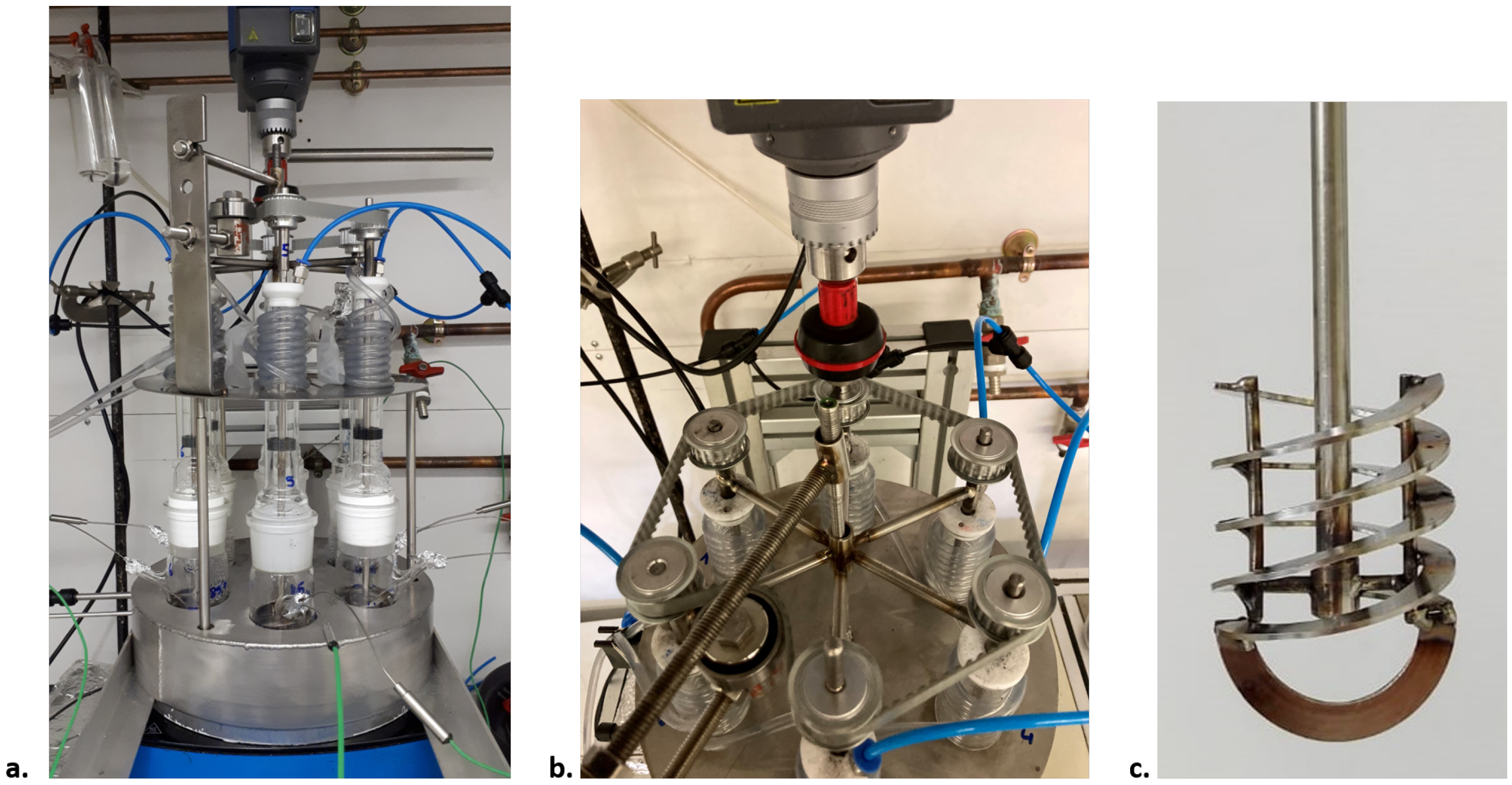
2.3. Medium-Sized System
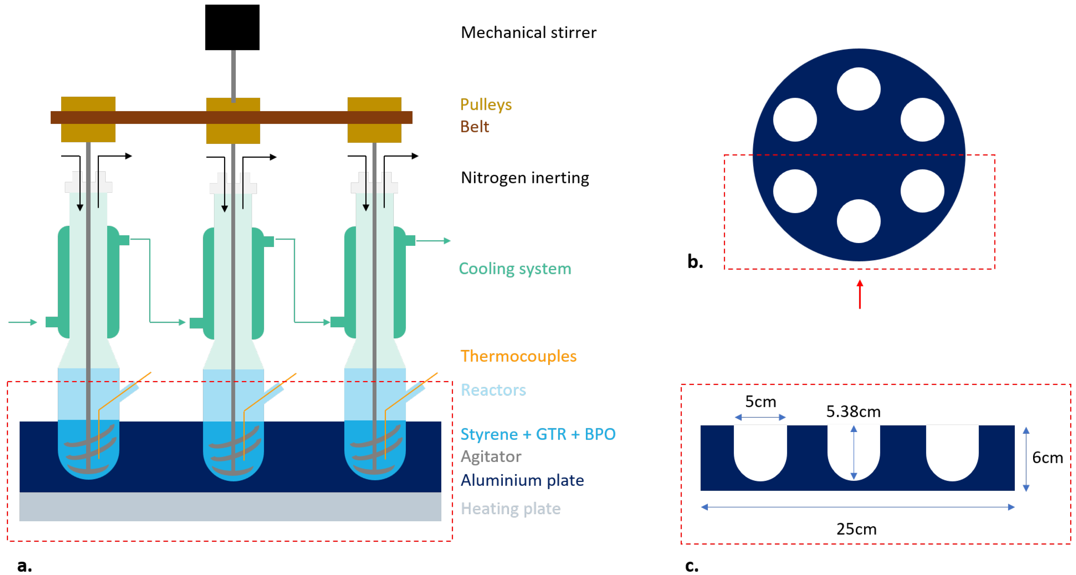
- The reactors were designed with a limited volume (<100 mL) to keep the duration of sample analysis after polymerization reasonable (note that the whole reactor content is analyzed) while enabling reactions with sufficient amounts of GTR. The collars are large enough to facilitate the introduction of the reactants and the recovery of the products, the latter being more or less viscous depending on the operating conditions. The reactor diameter remains constant along the reactor height (except the bottom). This facilitates the introduction and removal of the agitator. The reactor material (glass) facilitates the observation of the mixing conditions. Finally, a lateral orifice enables the punctual introduction of a thermocouple, inside the reactor, for temperature measurement.
- A 6-cm thick aluminum plate, containing 6 drilled reactor holdings, was used for reactor temperature control (Figure 1b,c). This plate was heated via conduction by an electrical heating plate on which it was directly placed. Silicon oil was also added in the holding positions to maximize the heat-transfer between the aluminum plate and the reactors.
- A cooling system was also installed at the upper part of the setup, enabling to cool down the vapors of monomer during the reaction. It was composed of a glass tube, positioned on top of each reactor and wrapped with a transparent hose in which circulated glycerol, at a temperature of to 3.5 °C, from a cooling thermostat bath.
- The mechanical agitator (Figure A1c) was designed with double propellers and an anchor to better scrape the reacting mixture from the walls and bottom of the reactors. In fact, since the mixture of GTR with PS became quite sticky during the polymerization, it was important to make sure that reactor content would remain under mixing throughout the polymerization, without forming an inverse bell shape with the agitator spinning in void in the middle of it. The rotation speed was fixed at 30 rpm. A pulley was fixed on the top of each stirring axe and a belt system made the 6 stirring axes rotate simultaneously (Figure A1b). The system was designed to keep the 6 axes parallel, thus avoiding stirrers from scratching and damaging the reactor walls.
- Nitrogen inerting, before the reactions, was also implemented via specifically designed inlets on the seals of the glass tubes and a dedicated nitrogen feeding network.
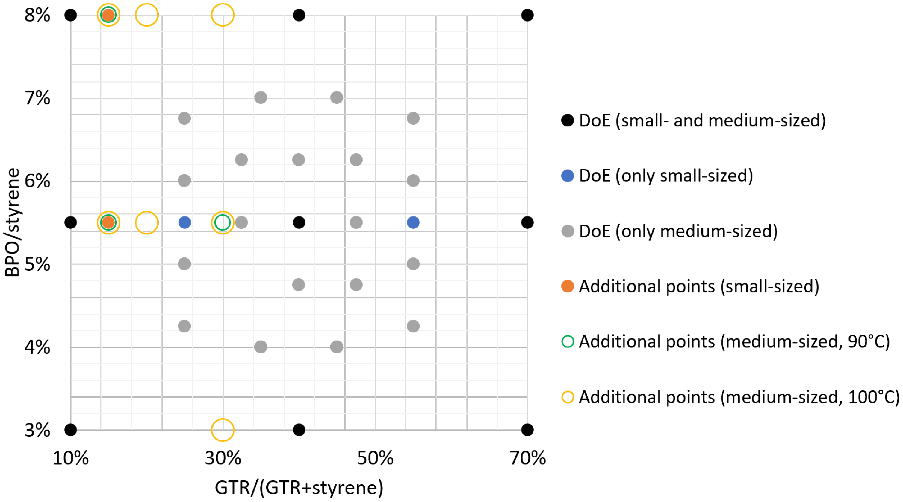
2.4. Design of Experiments
3. ML Modeling
3.1. ML Algorithms
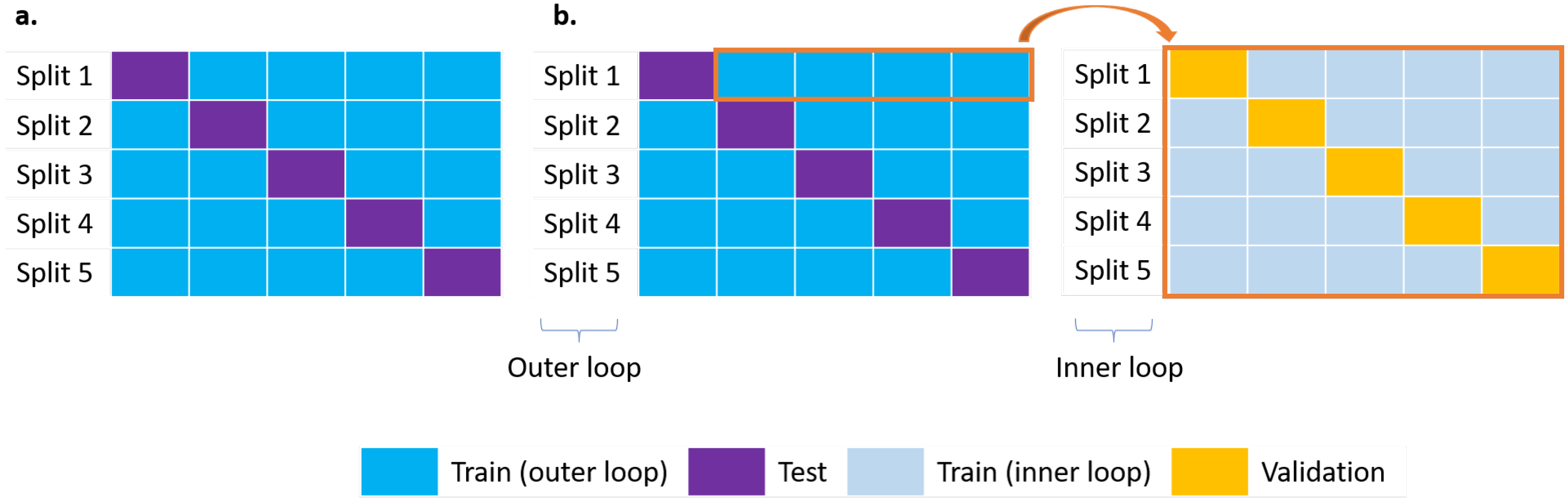
3.2. ML Procedure
4. Results and Discussion
4.1. Experimental Results
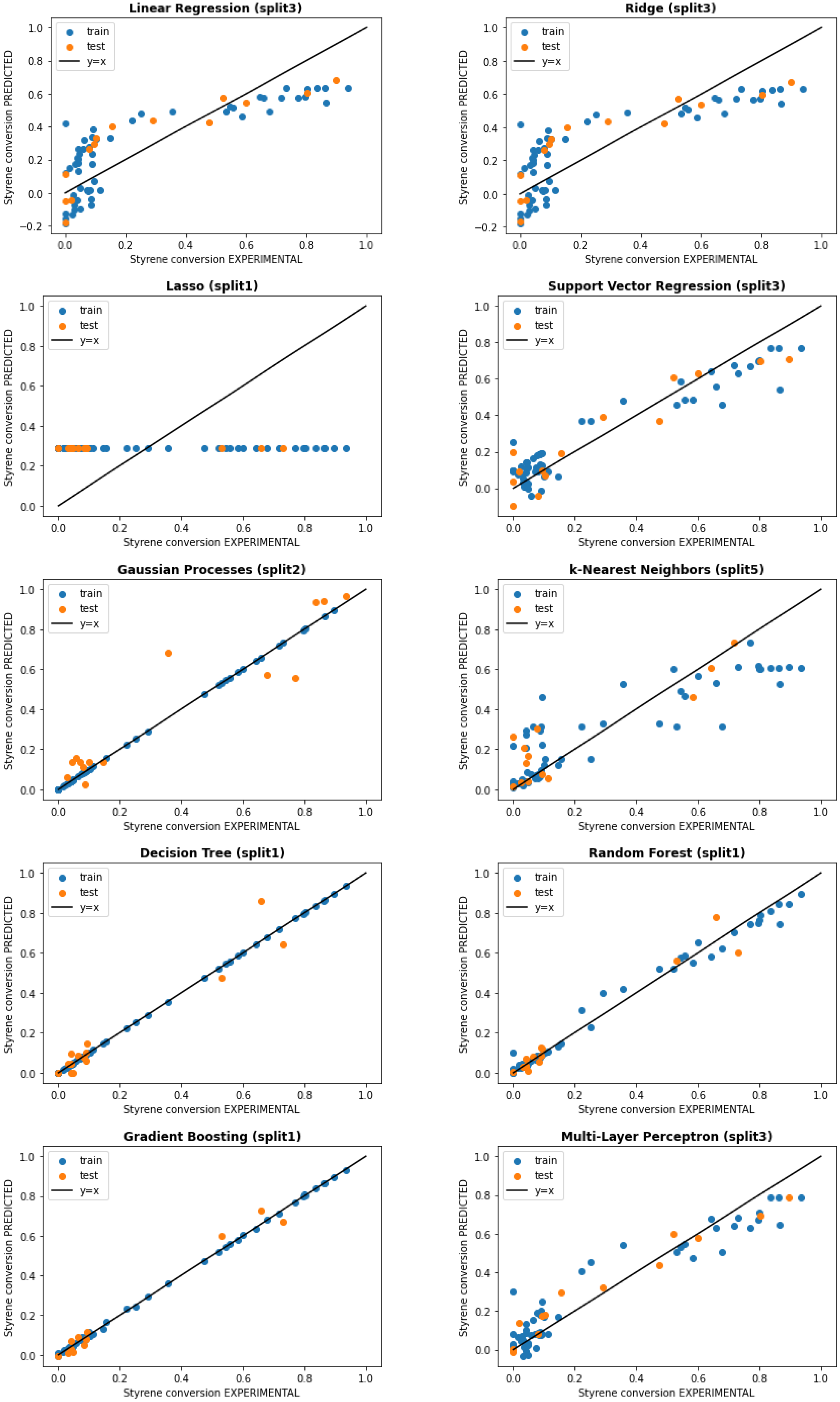
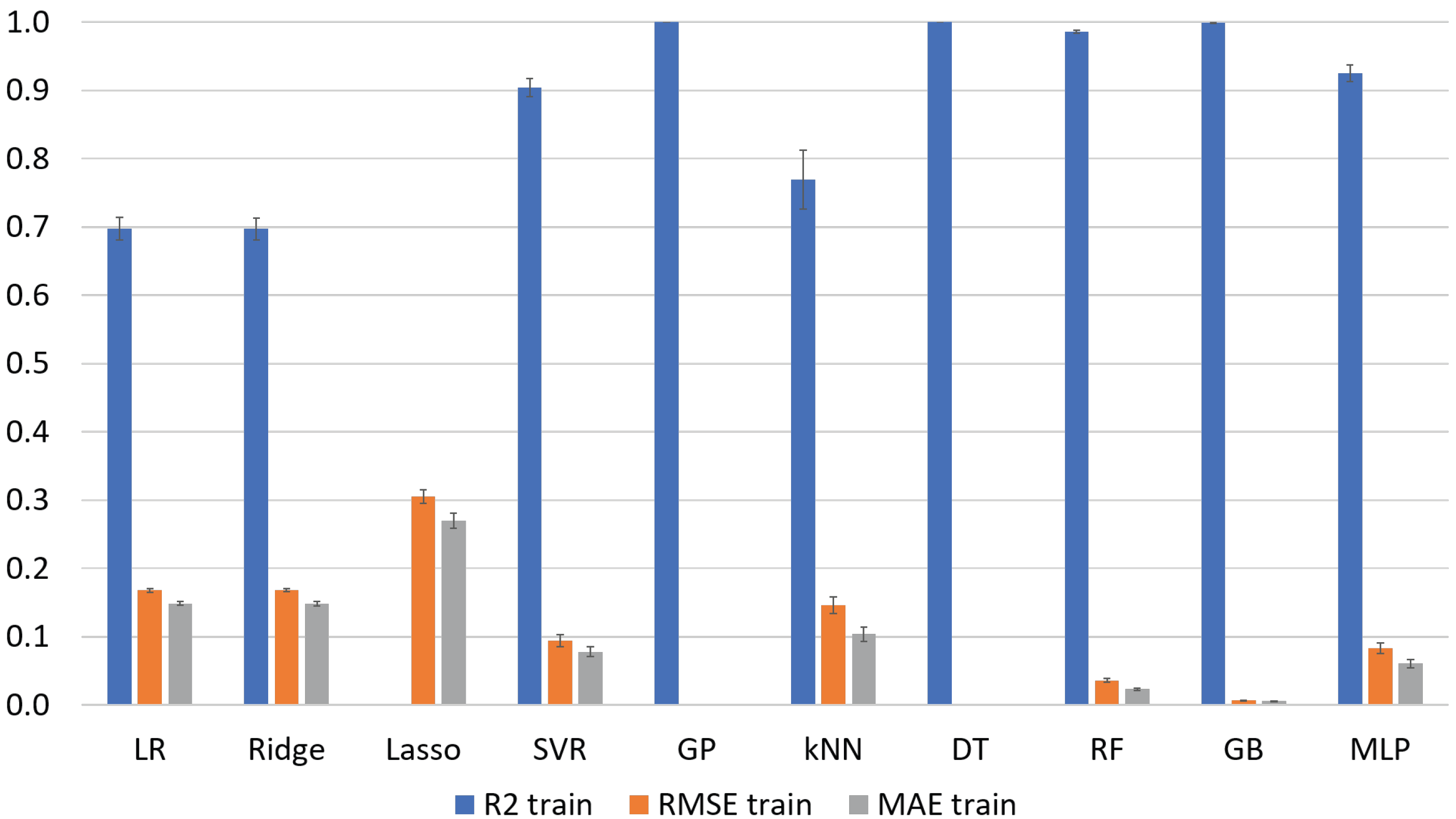
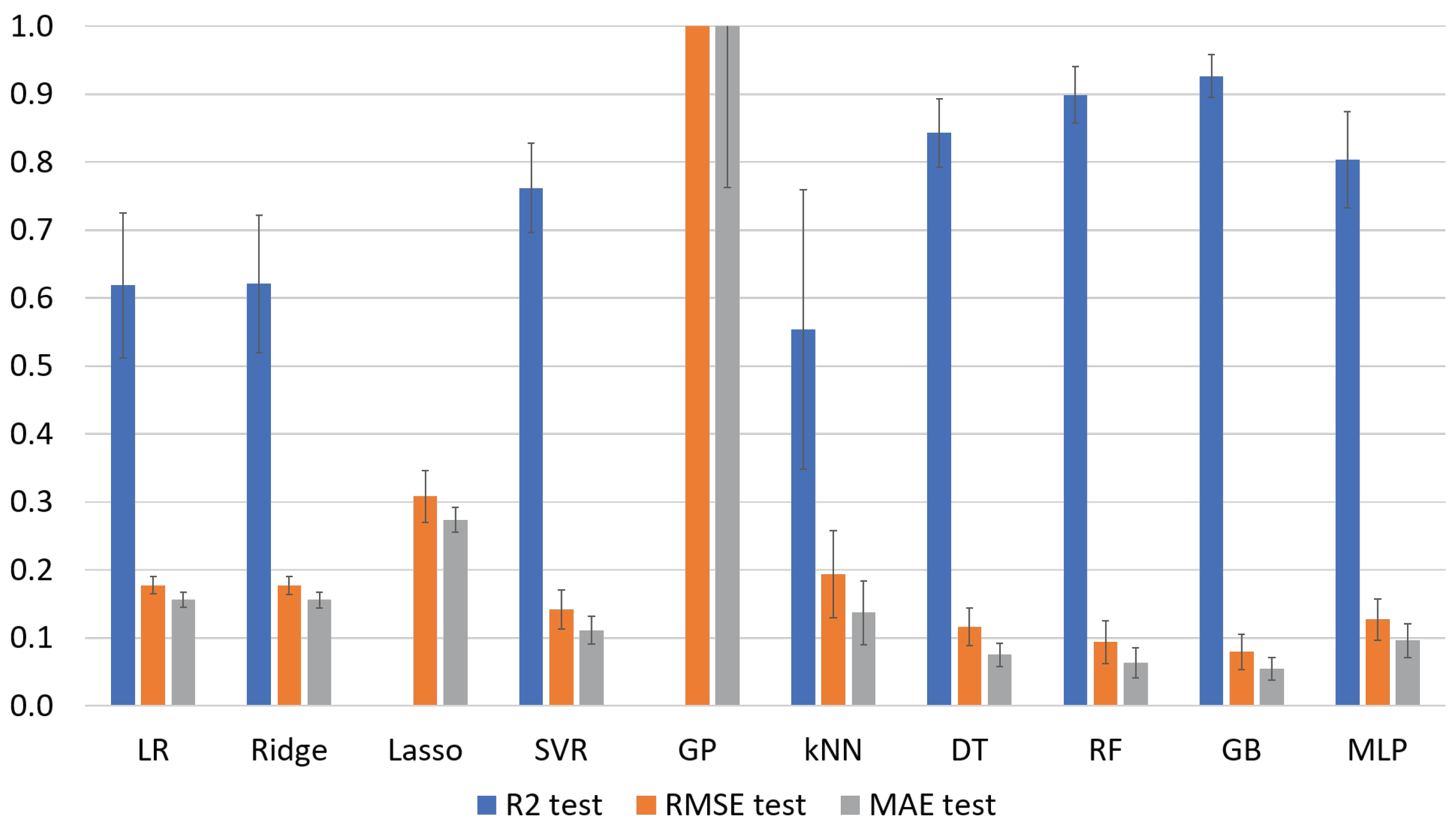
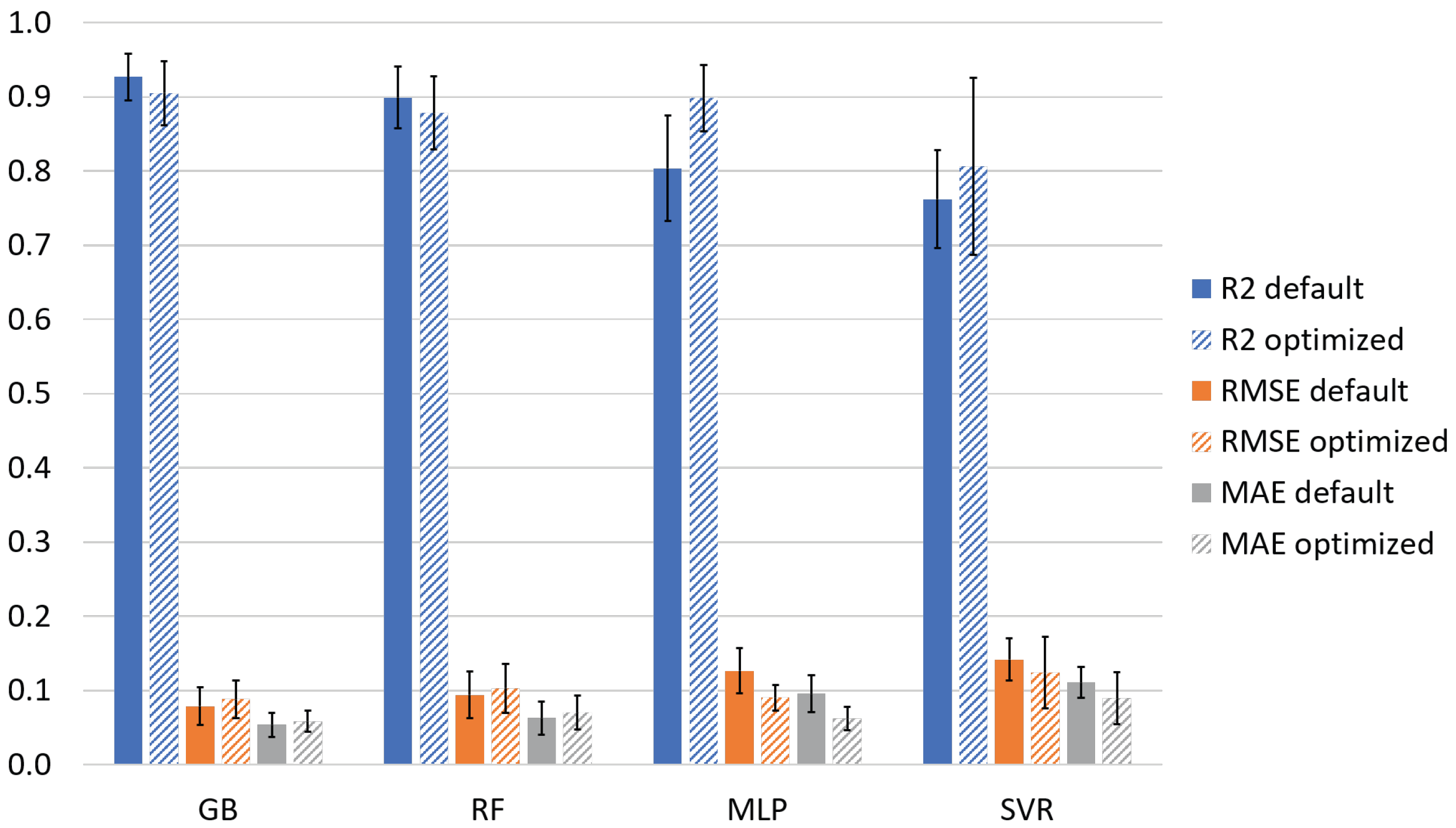
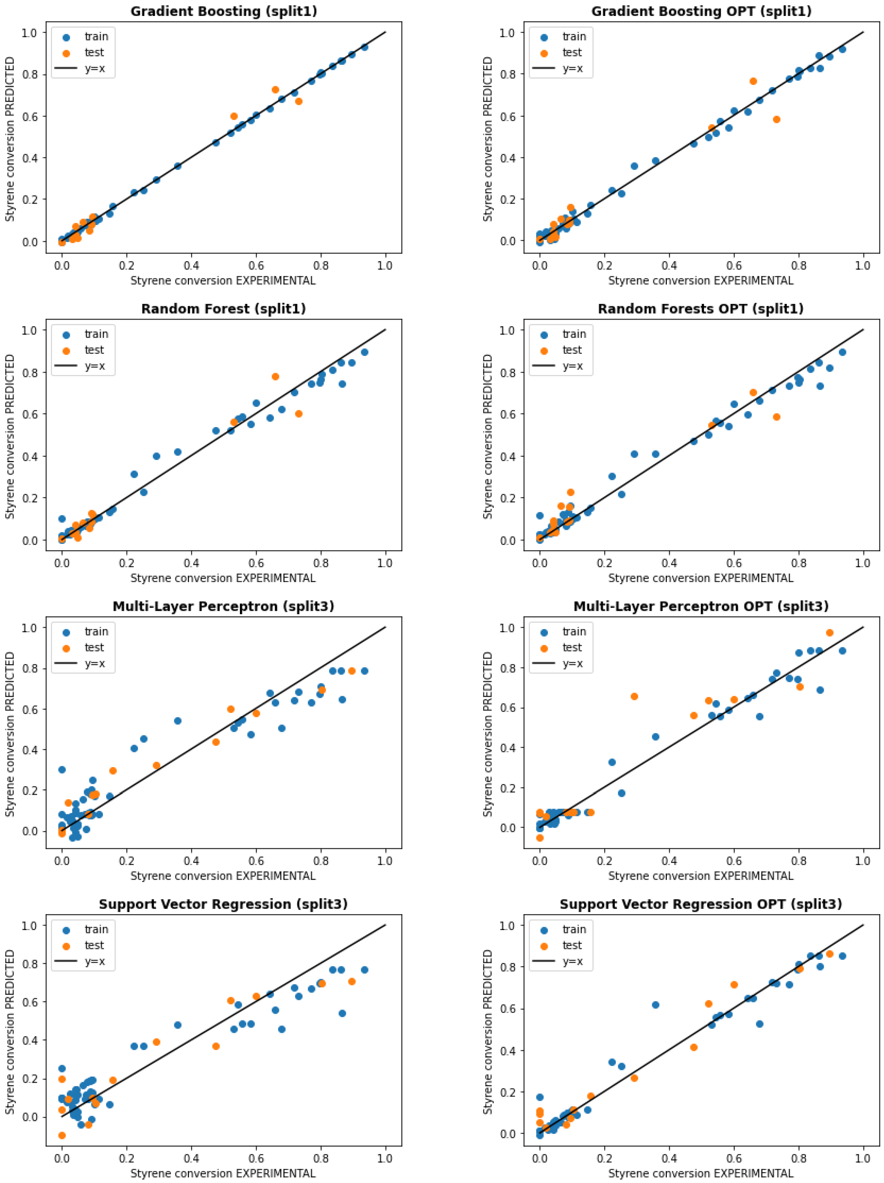
4.2. ML Results
5. Conclusions
Author Contributions
Funding
Data Availability Statement
Acknowledgments
Conflicts of Interest
Abbreviations
| ANN | Artificial neural networks |
| BPO | Benzoyl peroxide |
| DT | Decision trees |
| GB | Gradient boosting |
| GP | Gaussian processes |
| GTR | Ground tire rubber |
| HP | Hyperparameter |
| kNN | k-nearest neighbors |
| LR | Linear regression |
| MAE | Mean absolute error |
| ML | Machine learning |
| MLP | Multilayer perceptrons |
| PS | Polystyrene |
| RF | Random forest |
| RMSE | Root mean squared error |
| SVM | Support vector machines |
| SVR | Support vector regression |
Appendix A. Additional Photos of the Experimental Medium-Sized System

Appendix B. Evaluation of the Experimental Uncertainties
- is the loss of styrene during polymerization reaction due to evaporation;
- is the loss of styrene during the transfer of the reactor content to the gravimetry cup at the end of the polymerization;
- is the styrene remaining in the glass tube at the end of the polymerization reaction.
Appendix C. Detailed Experimental Data for the Small- and Medium-Sized Systems

| N° | Time, h | Temperature theo., °C | Temperature exp., °C | GTR/(GTR + Styrene) theo., %wt | GTR/(GTR + Styrene) exp., %wt | BPO/Styrene theo., %wt | BPO/Styrene exp., %wt | Conversion, %wt | Balance-Related Uncertainty, %wt |
|---|---|---|---|---|---|---|---|---|---|
| 1 | 2 | 90.0 | 89.0 | 10.00% | 10.23% | 5.50% | 5.49% | 47.57% | 0.13% |
| 2 | 2 | 90.0 | 89.0 | 40.00% | 40.35% | 5.50% | 5.49% | 0.00% | 0.13% |
| 3 | 2 | 90.0 | 89.0 | 70.00% | 69.94% | 5.50% | 5.49% | 0.00% | 0.07% |
| 4 | 5 | 90.0 | 89.0 | 10.00% | 9.79% | 5.50% | 5.49% | 58.41% | 0.13% |
| 5 | 5 | 90.0 | 89.0 | 40.00% | 40.06% | 5.50% | 5.49% | 1.49% | 0.11% |
| 6 | 5 | 90.0 | 89.0 | 70.00% | 69.87% | 5.50% | 5.49% | 0.00% | 0.08% |
| 7 | 8 | 90.0 | 89.0 | 10.00% | 9.79% | 3.00% | 2.99% | 28.97% | 0.08% |
| 8 | 8 | 90.0 | 89.0 | 10.00% | 10.28% | 5.50% | 5.55% | 67.84% | 0.10% |
| 9 | 8 | 90.0 | 89.0 | 10.00% | 10.16% | 5.50% | 5.49% | 53.13% | 0.08% |
| 10 | 8 | 90.0 | 89.0 | 10.00% | 10.00% | 8.00% | 8.03% | 86.53% | 0.08% |
| 11 | 8 | 90.0 | 89.0 | 15.00% | 15.03% | 5.50% | 5.49% | 22.05% | 0.08% |
| 12 | 8 | 90.0 | 89.0 | 15.00% | 14.98% | 8.00% | 8.03% | 35.60% | 0.08% |
| 13 | 8 | 90.0 | 89.0 | 25.00% | 24.99% | 5.50% | 5.51% | 8.94% | 0.09% |
| 14 | 8 | 90.0 | 89.0 | 40.00% | 40.01% | 3.00% | 2.99% | 4.36% | 0.15% |
| 15 | 8 | 90.0 | 89.0 | 40.00% | 41.65% | 5.50% | 5.77% | 3.42% | 0.11% |
| 16 | 8 | 90.0 | 89.0 | 40.00% | 40.13% | 5.50% | 5.49% | 4.25% | 0.11% |
| 17 | 8 | 90.0 | 89.0 | 40.00% | 40.11% | 8.00% | 8.00% | 8.81% | 0.11% |
| 18 | 8 | 90.0 | 89.0 | 55.00% | 54.96% | 5.50% | 5.51% | 4.86% | 0.14% |
| 19 | 8 | 90.0 | 89.0 | 70.00% | 69.97% | 3.00% | 2.99% | 0.00% | 0.31% |
| 20 | 8 | 90.0 | 89.0 | 70.00% | 71.68% | 5.50% | 5.94% | 2.45% | 0.13% |
| 21 | 8 | 90.0 | 89.0 | 70.00% | 69.95% | 5.50% | 5.49% | 0.00% | 0.13% |
| 22 | 8 | 90.0 | 89.0 | 70.00% | 69.95% | 8.00% | 8.00% | 8.55% | 0.21% |
| 23 | 2 | 100.0 | 99.3 | 10.00% | 10.42% | 5.50% | 5.75% | 55.66% | 0.21% |
| 24 | 2 | 100.0 | 99.3 | 40.00% | 40.20% | 5.50% | 5.50% | 4.18% | 0.11% |
| 25 | 2 | 100.0 | 99.3 | 70.00% | 70.15% | 5.50% | 5.50% | 3.00% | 0.11% |
| 26 | 5 | 100.0 | 99.3 | 10.00% | 10.02% | 5.50% | 5.50% | 59.96% | 0.21% |
| 27 | 5 | 100.0 | 99.3 | 40.00% | 40.20% | 5.50% | 5.50% | 4.72% | 0.11% |
| 28 | 5 | 100.0 | 99.3 | 70.00% | 70.05% | 5.50% | 5.50% | 3.13% | 0.08% |
| 29 | 8 | 100.0 | 99.3 | 10.00% | 9.98% | 3.00% | 3.01% | 54.50% | 0.29% |
| 30 | 8 | 100.0 | 99.3 | 10.00% | 10.44% | 5.50% | 5.79% | 71.82% | 0.15% |
| 31 | 8 | 100.0 | 99.3 | 10.00% | 9.99% | 5.50% | 5.50% | 77.12% | 0.11% |
| 32 | 8 | 100.0 | 99.3 | 10.00% | 9.98% | 8.00% | 7.99% | 80.12% | 0.13% |
| 33 | 8 | 100.0 | 99.3 | 15.00% | 15.01% | 8.00% | 7.99% | 52.21% | 0.08% |
| 34 | 8 | 100.0 | 99.3 | 25.00% | 25.08% | 5.50% | 5.48% | 0.00% | 0.08% |
| 35 | 8 | 100.0 | 99.3 | 40.00% | 40.05% | 3.00% | 3.01% | 3.99% | 0.08% |
| 36 | 8 | 100.0 | 99.3 | 40.00% | 40.59% | 5.50% | 5.70% | 5.94% | 0.08% |
| 37 | 8 | 100.0 | 99.3 | 40.00% | 40.25% | 5.50% | 5.50% | 7.93% | 0.08% |
| 38 | 8 | 100.0 | 99.3 | 40.00% | 40.08% | 8.00% | 8.01% | 6.35% | 0.13% |
| 39 | 8 | 100.0 | 99.3 | 55.00% | 55.01% | 5.50% | 5.48% | 0.00% | 0.11% |
| 40 | 8 | 100.0 | 99.3 | 70.00% | 70.02% | 3.00% | 3.01% | 4.87% | 0.11% |
| 41 | 8 | 100.0 | 99.3 | 70.00% | 70.41% | 5.50% | 5.75% | 4.15% | 0.13% |
| 42 | 8 | 100.0 | 99.3 | 70.00% | 70.53% | 5.50% | 5.50% | 0.00% | 0.21% |
| 43 | 8 | 100.0 | 99.3 | 70.00% | 69.99% | 8.00% | 8.01% | 7.58% | 0.21% |
| 44 | 2 | 110.0 | 107.0 | 10.00% | 10.06% | 5.50% | 5.50% | 65.74% | 0.21% |
| 45 | 2 | 110.0 | 107.0 | 40.00% | 40.06% | 5.50% | 5.50% | 4.25% | 0.11% |
| 46 | 2 | 110.0 | 107.0 | 70.00% | 69.96% | 5.50% | 5.50% | 1.98% | 0.08% |
| 47 | 5 | 110.0 | 107.0 | 10.00% | 9.96% | 5.50% | 5.50% | 80.32% | 0.21% |
| 48 | 5 | 110.0 | 107.0 | 40.00% | 40.07% | 5.50% | 5.50% | 9.50% | 0.11% |
| 49 | 5 | 110.0 | 107.0 | 70.00% | 70.12% | 5.50% | 5.50% | 2.72% | 0.08% |
| 50 | 8 | 110.0 | 107.0 | 10.00% | 10.33% | 3.00% | 3.00% | 79.60% | 0.29% |
| 51 | 8 | 110.0 | 107.0 | 10.00% | 10.10% | 5.50% | 5.58% | 93.55% | 0.14% |
| 52 | 8 | 110.0 | 107.0 | 10.00% | 10.01% | 5.50% | 5.50% | 86.15% | 0.11% |
| 53 | 8 | 110.0 | 107.0 | 10.00% | 10.02% | 5.50% | 5.49% | 83.63% | 0.21% |
| 54 | 8 | 110.0 | 107.0 | 10.00% | 10.72% | 8.00% | 8.00% | 89.71% | 0.11% |
| 55 | 8 | 110.0 | 107.0 | 15.00% | 15.04% | 5.50% | 5.49% | 64.39% | 0.08% |
| 56 | 8 | 110.0 | 107.0 | 15.00% | 15.07% | 8.00% | 8.00% | 73.23% | 0.08% |
| 57 | 8 | 110.0 | 107.0 | 25.00% | 25.08% | 5.50% | 5.49% | 25.18% | 0.13% |
| 58 | 8 | 110.0 | 107.0 | 32.50% | 32.56% | 5.50% | 5.50% | 15.51% | 0.10% |
| 59 | 8 | 110.0 | 107.0 | 40.00% | 40.01% | 3.00% | 3.00% | 7.86% | 0.08% |
| 60 | 8 | 110.0 | 107.0 | 40.00% | 39.59% | 5.50% | 5.42% | 10.27% | 0.08% |
| 61 | 8 | 110.0 | 107.0 | 40.00% | 40.07% | 5.50% | 5.50% | 14.69% | 0.09% |
| 62 | 8 | 110.0 | 107.0 | 40.00% | 40.07% | 5.50% | 5.49% | 10.11% | 0.09% |
| 63 | 8 | 110.0 | 107.0 | 40.00% | 39.87% | 8.00% | 8.00% | 9.33% | 0.11% |
| 64 | 8 | 110.0 | 107.0 | 55.00% | 55.04% | 5.50% | 5.49% | 8.92% | 0.11% |
| 65 | 8 | 110.0 | 107.0 | 70.00% | 69.96% | 3.00% | 3.00% | 8.62% | 0.11% |
| 66 | 8 | 110.0 | 107.0 | 70.00% | 70.32% | 5.50% | 5.63% | 7.22% | 0.14% |
| 67 | 8 | 110.0 | 107.0 | 70.00% | 69.99% | 5.50% | 5.50% | 11.42% | 0.21% |
| 68 | 8 | 110.0 | 107.0 | 70.00% | 70.00% | 5.50% | 5.49% | 8.12% | 0.21% |
| 69 | 8 | 110.0 | 107.0 | 70.00% | 70.08% | 8.00% | 8.00% | 9.45% | 0.21% |
| N° | Time, h | Temperature theo., °C | Temperature exp., °C | GTR/(GTR + Styrene) theo., %wt | GTR/(GTR + Styrene) exp., %wt | BPO/Styrene theo., %wt | BPO/Styrene exp., %wt | Conversion, %wt | Balance-Related Uncertainty, %wt |
|---|---|---|---|---|---|---|---|---|---|
| 1 | 90 | 94.6 | >98.16 | 10.00% | 10.20% | 3.00% | 3.04% | 18.43% | 0.12% |
| 2 | 90 | 93.4 | >98.45 | 10.00% | 10.15% | 3.00% | 3.01% | 14.40% | 0.12% |
| 3 | 90 | 93.8 | >109.47 | 10.00% | 10.19% | 5.50% | 5.58% | 49.20% | 0.12% |
| 4 | 90 | na | na | 10.00% | 10.66% | 5.50% | 5.89% | 37.88% | 0.14% |
| 5 | 90 | 92.2 | >93 | 10.00% | 10.15% | 5.50% | 5.57% | 49.93% | 0.13% |
| 6 | 90 | 92.9 | >146.30 | 10.00% | 10.19% | 8.00% | 8.08% | 72.52% | 0.12% |
| 7 | 90 | 95.7 | >136.95 | 10.00% | 10.28% | 8.00% | 8.16% | 72.53% | 0.12% |
| 8 | 90 | 91.9 | >94 | 15.00% | 15.24% | 5.50% | 5.54% | 10.40% | 0.13% |
| 9 | 90 | 92.3 | >109.77 | 15.00% | 15.25% | 8.00% | 8.07% | 24.20% | 0.13% |
| 10 | 90 | 96.7 | >115.47 | 25.00% | 25.77% | 4.25% | 4.37% | 6.11% | 0.21% |
| 11 | 90 | 95 | >97.03 | 25.00% | 25.60% | 5.00% | 5.13% | 5.75% | 0.21% |
| 12 | 90 | 93.9 | >95.97 | 25.00% | 25.38% | 6.00% | 6.09% | 5.03% | 0.21% |
| 13 | 90 | 93.9 | >94.72 | 25.00% | 25.35% | 6.75% | 6.83% | 6.23% | 0.21% |
| 14 | 90 | na | na | 30.00% | 30.47% | 5.50% | 5.56% | 2.75% | 0.22% |
| 15 | 90 | 90.5 | >91 | 30.00% | 30.37% | 5.50% | 5.51% | 2.64% | 0.22% |
| 16 | 90 | 92.5 | >93.30 | 40.00% | 40.47% | 5.50% | 5.54% | 3.54% | 0.35% |
| 17 | 90 | 90.7 | >95.85 | 40.00% | 40.73% | 8.00% | 8.16% | 5.39% | 0.35% |
| 18 | 90 | na | na | 70.00% | 72.46% | 5.50% | 5.88% | 6.99% | 1.19% |
| 19 | 90 | 89.2 | >92 | 70.00% | 73.21% | 5.50% | 6.32% | 5.87% | 1.22% |
| 20 | 100 | 103.6 | >105.69 | 10.00% | 10.18% | 3.00% | 3.04% | 45.04% | 0.12% |
| 21 | 100 | 104.4 | >123.65 | 10.00% | 10.20% | 5.50% | 5.56% | 69.92% | 0.12% |
| 22 | 100 | 103.9 | >129.84 | 10.00% | 10.62% | 8.00% | 8.45% | 91.82% | 0.13% |
| 23 | 100 | 102.6 | >143.30 | 10.00% | 10.32% | 8.00% | 8.20% | 78.12% | 0.13% |
| 24 | 100 | 102.2 | >118.83 | 10.00% | 10.16% | 8.00% | 8.08% | 83.37% | 0.13% |
| 25 | 100 | 103 | >104.38 | 15.00% | 15.20% | 5.50% | 5.49% | 19.42% | 0.13% |
| 26 | 100 | na | na | 15.00% | 15.22% | 5.50% | 5.53% | 18.57% | 0.13% |
| 27 | 100 | 101.7 | >109.85 | 15.00% | 15.23% | 8.00% | 8.08% | 36.72% | 0.13% |
| 28 | 100 | na | na | 20.00% | 21.86% | 5.50% | 6.11% | 6.61% | 0.14% |
| 29 | 100 | 104 | >105 | 20.00% | 20.24% | 5.50% | 5.57% | 9.81% | 0.13% |
| 30 | 100 | 102 | >103.96 | 20.00% | 20.28% | 8.00% | 8.07% | 12.43% | 0.14% |
| 31 | 100 | 106 | >106.85 | 25.00% | 25.52% | 4.25% | 4.31% | 16.18% | 0.20% |
| 32 | 100 | 103.7 | >104.90 | 25.00% | 25.12% | 5.00% | 4.99% | 9.70% | 0.21% |
| 33 | 100 | 104.3 | >105.29 | 25.00% | 25.17% | 5.00% | 5.03% | 12.52% | 0.20% |
| 34 | 100 | 100.2 | >106.49 | 25.00% | 25.34% | 6.00% | 6.05% | 6.07% | 0.18% |
| 35 | 100 | 104.5 | >105.65 | 25.00% | 25.36% | 6.00% | 6.06% | 8.68% | 0.18% |
| 36 | 100 | 106.7 | >115.21 | 25.00% | 26.05% | 6.75% | 7.06% | 16.49% | 0.21% |
| 37 | 100 | na | na | 30.00% | 30.05% | 3.00% | 3.01% | 4.13% | 0.20% |
| 38 | 100 | 101.4 | >103 | 30.00% | 30.33% | 3.00% | 3.00% | 3.85% | 0.21% |
| 39 | 100 | na | na | 30.00% | 30.30% | 5.50% | 5.53% | 5.02% | 0.21% |
| 40 | 100 | 101.1 | >103 | 30.00% | 30.40% | 5.50% | 5.56% | 4.58% | 0.21% |
| 41 | 100 | na | na | 30.00% | 30.24% | 8.00% | 8.05% | 4.77% | 0.21% |
| 42 | 100 | 100.4 | >103 | 30.00% | 30.72% | 8.00% | 8.19% | 6.15% | 0.21% |
| 43 | 100 | 103.3 | >105.66 | 32.50% | 33.32% | 5.50% | 5.63% | 6.43% | 0.27% |
| 44 | 100 | 103.3 | >104.14 | 32.50% | 32.73% | 6.25% | 6.25% | 7.49% | 0.26% |
| 45 | 100 | 101.9 | >105.63 | 35.00% | 36.84% | 4.00% | 4.30% | 5.30% | 0.28% |
| 46 | 100 | 103.8 | >105.61 | 35.00% | 35.92% | 7.00% | 7.19% | 7.74% | 0.28% |
| 47 | 100 | 101.6 | >105.65 | 40.00% | 40.43% | 3.00% | 3.03% | 5.48% | 0.35% |
| 48 | 100 | na | na | 40.00% | 40.75% | 5.50% | 5.63% | 4.37% | 0.34% |
| 49 | 100 | 99.6 | >101 | 40.00% | 40.62% | 5.50% | 5.56% | 4.20% | 0.33% |
| 50 | 100 | 104.5 | >106.32 | 40.00% | 41.69% | 6.25% | 6.55% | 8.69% | 0.36% |
| 51 | 100 | 102 | >102.70 | 40.00% | 40.90% | 8.00% | 8.13% | 7.79% | 0.36% |
| 52 | 100 | na | na | 70.00% | 72.44% | 5.50% | 6.05% | 8.07% | 1.14% |
| 53 | 100 | 101.2 | >102 | 70.00% | 72.69% | 5.50% | 6.00% | 8.43% | 1.15% |
| 54 | 100 | 99.4 | >103.70 | 70.00% | 73.56% | 8.00% | 9.16% | 12.16% | 1.30% |
| 55 | 110 | 114.8 | >115.40 | 25.00% | 25.25% | 4.25% | 4.18% | 22.11% | 0.20% |
| 56 | 110 | 112.8 | >113.52 | 25.00% | 25.25% | 5.00% | 5.04% | 18.17% | 0.20% |
| 57 | 110 | 112.9 | >113.60 | 25.00% | 25.17% | 6.75% | 6.78% | 20.68% | 0.20% |
| 58 | 110 | 112.9 | >113.74 | 32.50% | 32.94% | 5.50% | 5.52% | 10.84% | 0.26% |
| 59 | 110 | 113.3 | >114.45 | 32.50% | 33.11% | 6.25% | 6.29% | 11.44% | 0.26% |
| 60 | 110 | 113.7 | >114.96 | 35.00% | 35.91% | 7.00% | 7.16% | 13.46% | 0.33% |
Appendix D. Detailed ML Results
| ML Algorithm | Train | Test | RMSE Train | Test | MAE Train | Test |
|---|---|---|---|---|---|---|
| LR | 0.697 ± 0.016 | 0.619 ± 0.107 | 0.168 ± 0.003 | 0.177 ± 0.013 | 0.148 ± 0.003 | 0.156 ± 0.011 |
| Ridge | 0.697 ± 0.016 | 0.621 ± 0.101 | 0.168 ± 0.003 | 0.177 ± 0.013 | 0.148 ± 0.003 | 0.156 ± 0.012 |
| Lasso | 0.000 ± 0.000 | −0.096 ± 0.069 | 0.306 ± 0.010 | 0.308 ± 0.038 | 0.270 ± 0.011 | 0.273 ± 0.018 |
| SVR | 0.905 ± 0.013 | 0.762 ± 0.066 | 0.094 ± 0.009 | 0.142 ± 0.029 | 0.078 ± 0.007 | 0.111 ± 0.021 |
| GP | 1.000 ± 0.000 | −1736 ± 1572 | 0.000 ± 0.000 | 8.644 ± 6.903 | 0.000 ± 0.000 | 3.592 ± 2.829 |
| kNN | 0.769 ± 0.043 | 0.554 ± 0.206 | 0.146 ± 0.012 | 0.193 ± 0.064 | 0.104 ± 0.011 | 0.137 ± 0.047 |
| DT | 1.000 ± 0.000 | 0.843 ± 0.050 | 0.000 ± 0.000 | 0.116 ± 0.027 | 0.000 ± 0.000 | 0.075 ± 0.017 |
| RF | 0.986 ± 0.002 | 0.899 ± 0.042 | 0.036 ± 0.003 | 0.094 ± 0.031 | 0.023 ± 0.002 | 0.063 ± 0.022 |
| GB | 1.000 ± 0.000 | 0.927 ± 0.032 | 0.007 ± 0.000 | 0.079 ± 0.026 | 0.005 ± 0.000 | 0.054 ± 0.016 |
| MLP | 0.925 ± 0.012 | 0.804 ± 0.071 | 0.083 ± 0.008 | 0.127 ± 0.030 | 0.061 ± 0.006 | 0.096 ± 0.025 |
| SVR | RF | GB | MLP | |
|---|---|---|---|---|
| train | 0.959 ± 0.019 | 0.985 ± 0.002 | 0.996 ± 0.002 | 0.992 ± 0.008 |
| test | 0.806 ± 0.119 | 0.878 ± 0.049 | 0.905 ± 0.043 | 0.898 ± 0.045 |
| RMSE train | 0.061 ± 0.015 | 0.038 ± 0.003 | 0.018 ± 0.005 | 0.025 ± 0.012 |
| RMSE test | 0.124 ± 0.048 | 0.103 ± 0.033 | 0.088 ± 0.025 | 0.090 ± 0.017 |
| MAE train | 0.031 ± 0.007 | 0.025 ± 0.002 | 0.014 ± 0.003 | 0.016 ± 0.009 |
| MAE test | 0.090 ± 0.035 | 0.070 ± 0.023 | 0.059 ± 0.014 | 0.062 ± 0.016 |
Appendix E. Ways of Improvement for the ML Model


References
- Abbas-Abadi, M.S.; Kusenberg, M.; Shirazi, H.M.; Goshayeshi, B.; Van Geem, K.M. Towards full recyclability of end-of-life tires: Challenges and opportunities. J. Clean. Prod. 2022, 374, 134036. [Google Scholar] [CrossRef]
- Hejna, A.; Korol, J.; Przybysz-Romatowska, M.; Zedler, Ł.; Chmielnicki, B.; Formela, K. Waste tire rubber as low-cost and environmentally-friendly modifier in thermoset polymers—A review. Waste Manag. 2020, 108, 106–118. [Google Scholar] [CrossRef] [PubMed]
- Fazli, A.; Rodrigue, D. Recycling waste tires into ground tire rubber (Gtr)/rubber compounds: A review. J. Compos. Sci. 2020, 4, 103. [Google Scholar] [CrossRef]
- Ramarad, S.; Khalid, M.; Ratnam, C.T.; Chuah, A.L.; Rashmi, W. Waste tire rubber in polymer blends: A review on the evolution, properties and future. Prog. Mater. Sci. 2015, 72, 100–140. [Google Scholar] [CrossRef]
- Araujo-Morera, J.; Verdugo-Manzanares, R.; González, S.; Verdejo, R.; Lopez-Manchado, M.A.; Santana, M.H. On the use of mechano-chemically modified ground tire rubber (Gtr) as recycled and sustainable filler in styrene-butadiene rubber (sbr) composites. J. Compos. Sci. 2021, 5, 68. [Google Scholar] [CrossRef]
- Phiri, M.M.; Phiri, M.J.; Formela, K.; Wang, S.; Hlangothi, S.P. Grafting and reactive extrusion technologies for compatibilization of ground tyre rubber composites: Compounding, properties, and applications. J. Clean. Prod. 2022, 369, 133084. [Google Scholar] [CrossRef]
- Colom, X.; Cañavate, J.; Carrillo-Navarrete, F. Towards Circular Economy by the Valorization of Different Waste Subproducts through Their Incorporation in Composite Materials: Ground Tire Rubber and Chicken Feathers. Polymers 2022, 14, 1090. [Google Scholar] [CrossRef]
- He, M.; Gu, K.; Wang, Y.; Li, Z.; Shen, Z.; Liu, S.; Wei, J. Development of high-performance thermoplastic composites based on polyurethane and ground tire rubber by in-situ synthesis. Resour. Conserv. Recycl. 2021, 173, 105713. [Google Scholar] [CrossRef]
- Archibong, F.N.; Sanusi, O.M.; Médéric, P.; Hocine, N.A. An overview on the recycling of waste ground tyre rubbers in thermoplastic matrices: Effect of added fillers. Resour. Conserv. Recycl. 2021, 175, 105894. [Google Scholar] [CrossRef]
- Liu, S.; Peng, Z.; Zhang, Y.; Rodrigue, D.; Wang, S. Compatibilized thermoplastic elastomers based on highly filled polyethylene with ground tire rubber. J. Appl. Polym. Sci. 2022, 139, e52999. [Google Scholar] [CrossRef]
- Fan, P.; Lu, C. Surface Graft Copolymerization of Poly(methyl methacrylate) onto Waste Tire Rubber Powder through Ozonization. J. Appl. Polym. Sci. 2011, 122, 2262–2270. [Google Scholar] [CrossRef]
- Coiai, S.; Passaglia, E.; Ciardelli, F.; Tirelli, D.; Peruzzotti, F.; Resmini, E. Modification of cross-linked rubber particles by free radical polymerization. Macromol. Symp. 2006, 234, 193–202. [Google Scholar] [CrossRef]
- Sulcis, R.; Lotti, L.; Coiai, S.; Ciardelli, F.; Passaglia, E. Novel HDPE/ground tyre rubber composite materials obtained through in-situ polymerization and polymerization filling technique. J. Appl. Polym. Sci. 2014, 131, 1–13. [Google Scholar] [CrossRef]
- Sulcis, R.; Vizza, F.; Oberhauser, W.; Ciardelli, F.; Spiniello, R.; Dintcheva, N.T.; Passaglia, E. Recycling ground tire rubber (GTR) scraps as high-impact filler of in situ produced polyketone matrix. Polym. Adv. Technol. 2014, 25, 1060–1068. [Google Scholar] [CrossRef]
- Tsagkalias, I.S.; Vlachou, A.; Verros, G.D.; Achilias, D.S. Effect of graphene oxide or functionalized graphene oxide on the copolymerization kinetics of Styrene/n-butyl methacrylate. Polymers 2019, 11, 999. [Google Scholar] [CrossRef] [PubMed] [Green Version]
- Potts, J.R.; Lee, S.H.; Alam, T.M.; An, J.; Stoller, M.D.; Piner, R.D.; Ruoff, R.S. Thermomechanical properties of chemically modified graphene/poly(methyl methacrylate) composites made by in situ polymerization. Carbon 2011, 49, 2615–2623. [Google Scholar] [CrossRef]
- Tripathi, S.N.; Saini, P.; Gupta, D.; Choudhary, V. Electrical and mechanical properties of PMMA/reduced graphene oxide nanocomposites prepared via in situ polymerization. J. Mater. Sci. 2013, 48, 6223–6232. [Google Scholar] [CrossRef]
- Wang, J.; Hu, H.; Wang, X.; Xu, C.; Zhang, M.; Shang, X. Preparation and Mechanical and Electrical Properties of Graphene Nanosheets–Poly(methyl methacrylate) Nanocomposites via In Situ Suspension Polymerization Jingchao. J. Appl. Polym. Sci. 2011, 122, 1866–1871. [Google Scholar] [CrossRef]
- Feng, L.; Guan, G.; Li, C.; Zhang, D.; Xiao, Y.; Zheng, L.; Zhu, W. In situ synthesis of poly(methyl methacrylate)/graphene oxide nanocomposites using thermal-initiated and graphene oxide-initiated polymerization. J. Macromol. Sci. Part A Pure Appl. Chem. 2013, 50, 720–727. [Google Scholar] [CrossRef]
- Michailidis, M.; Verros, G.D.; Deliyanni, E.A.; Andriotis, E.G.; Achilias, D.S. An experimental and theoretical study of butyl methacrylate in situ radical polymerization kinetics in the presence of graphene oxide nanoadditive. J. Polym. Sci. Part A Polym. Chem. 2017, 55, 1433–1441. [Google Scholar] [CrossRef]
- Tsagkalias, I.S.; Papadopoulou, S.; Verros, G.D.; Achilias, D.S. Polymerization Kinetics of n-Butyl Methacrylate in the Presence of Graphene Oxide Prepared by Two Different Oxidation Methods with or without Functionalization. Ind. Eng. Chem. Res. 2018, 57, 2449–2460. [Google Scholar] [CrossRef]
- Funck, A.; Kaminsky, W. Polypropylene carbon nanotube composites by in situ polymerization. Compos. Sci. Technol. 2007, 67, 906–915. [Google Scholar] [CrossRef]
- Jiang, X.; Bin, Y.; Matsuo, M. Electrical and mechanical properties of polyimide-carbon nanotubes composites fabricated by in situ polymerization. Polymer 2005, 46, 7418–7424. [Google Scholar] [CrossRef]
- Verros, G.D.; Achilias, D.S. Toward the development of a mathematical model for the bulk in situ radical polymerization of methyl methacrylate in the presence of nano-additives. Can. J. Chem. Eng. 2016, 94, 1783–1791. [Google Scholar] [CrossRef]
- Yeh, J.M.; Liou, S.J.; Lai, M.C.; Chang, Y.W.; Huang, C.Y.; Chen, C.P.; Jaw, J.H.; Tsai, T.Y.; Yu, Y.H. Comparative studies of the properties of poly(methyl methacrylate)-clay nanocomposite materials prepared by in situ emulsion polymerization and solution dispersion. J. Appl. Polym. Sci. 2004, 94, 1936–1946. [Google Scholar] [CrossRef]
- Meng, X.; Wu, H.; Storti, G.; Morbidelli, M. Effect of Dispersed Polymeric Nanoparticles on the Bulk Polymerization of Methyl Methacrylate. Macromolecules 2016, 49, 7758–7766. [Google Scholar] [CrossRef]
- Florez, D.; Hoppe, S.; Hu, G.H.; Meimaroglou, D. Radical bulk polymerization of styrene in the presence of rubber particles from recycled tires: A kinetic study using DSC. J. Therm. Anal. Calorim. 2020, 143, 3073–3084. [Google Scholar] [CrossRef]
- Parra, D.C.F. Effects of the Presence of Recycled Tire Powders on the Kinetics of the Radical Polymerization of Styrene and the Properties of the Resulting Materials. Ph.D. Thesis, Université de Lorraine, Lorraine, France, 2019; pp. 1–197. [Google Scholar]
- Meimaroglou, D.; Florez, D.; Hu, G.H. A kinetic modeling framework for the peroxide-initiated radical polymerization of styrene in the presence of rubber particles from recycled tires. Chem. Eng. Sci. 2022, 248, 117137. [Google Scholar] [CrossRef]
- Cameron, G.G.; Qureshi, M.Y. Free Radical Grafting of Monomers to Polydienes–4. Kinetics and Mechanism of Methyl Methacrylate Grafting to Polybutadiene. J. Polym. Sci. Part A 1 Polym. Chem. 1980, 18, 3149–3161. [Google Scholar] [CrossRef]
- Estenoz, D.A.; Meira, G.R.; Gomez, N.; Oliva, H.M. Mathematical model of a continuous industrial high-impact polystyrene process. AIChE J. 1998, 44, 427–441. [Google Scholar] [CrossRef]
- Meira, G.R.; Luciani, C.V.; Estenoz, D.A. Continuous Bulk Process for the Production of High-Impact Polystyrene: Recent Developments in Modeling and Control. Macromol. React. Eng. 2007, 1, 25–39. [Google Scholar] [CrossRef]
- Zhu, C.X.; Wu, Y.Y.; Figueira, F.L.; Van Steenberge, P.H.; D’hooge, D.R.; Zhou, Y.N.; Luo, Z.H. Sensitivity analysis of isothermal free radical induced grafting through application of the distribution—Numerical fractionation—Method of moments. Chem. Eng. J. 2022, 444, 136595. [Google Scholar] [CrossRef]
- Xu, P.; Chen, H.; Li, M.; Lu, W. New Opportunity: Machine Learning for Polymer Materials Design and Discovery. Adv. Theory Simul. 2022, 5, 2100565. [Google Scholar] [CrossRef]
- Trinh, C.; Meimaroglou, D.; Hoppe, S. Machine learning in chemical product engineering: The state of the art and a guide for newcomers. Processes 2021, 9, 1456. [Google Scholar] [CrossRef]
- Zhang, J.L.; Chen, H.X.; Ke, C.M.; Zhou, Y.; Lu, H.Z.; Wang, D.L. Graft polymerization of styrene onto waste rubber powder and surface characterization of graft copolymer. Polym. Bull. 2012, 68, 789–801. [Google Scholar] [CrossRef]
- Fazli, A.; Rodrigue, D. Effect of ground tire rubber (Gtr) particle size and content on the morphological and mechanical properties of recycled high-density polyethylene (rhdpe)/gtr blends. Recycling 2021, 6, 44. [Google Scholar] [CrossRef]
- Zhang, J.; Chen, H.; Zhou, Y.; Ke, C.; Lu, H. Compatibility of waste rubber powder/polystyrene blends by the addition of styrene grafted styrene butadiene rubber copolymer: Effect on morphology and properties. Polym. Bull. 2013, 70, 2829–2841. [Google Scholar] [CrossRef]
- Aggarwal, P.K.; Karmarkar, A.; Taqui, S.N. Grafting of Styrene Onto Cellulose. Int. Res. J. Eng. Technol. 2018, 2, 1081–1089. [Google Scholar]
- Hejna, A.; Klein, M.; Saeb, M.R.; Formela, K. Towards understanding the role of peroxide initiators on compatibilization efficiency of thermoplastic elastomers highly filled with reclaimed GTR. Polym. Test. 2019, 73, 143–151. [Google Scholar] [CrossRef]
- Liu, H.L.; Wang, X.P.; Jia, D.M. Recycling of waste rubber powder by mechano-chemical modification. J. Clean. Prod. 2020, 245, 118716. [Google Scholar] [CrossRef]
- Fletes, R.C.; López, E.O.; Gudiño, P.O.; Mendizábal, E.; Núñez, R.G.; Rodrigue, D. Ground tire rubber/polyamide 6 thermoplastic elastomers produced by dry blending and compression molding. Prog. Rubber Plast. Recycl. Technol. 2022, 38, 38–55. [Google Scholar] [CrossRef]
- Ku, H. Notes on the use of propagation of error formulas. J. Res. Natl. Bur. Stand. Sect. C Eng. Instrum. 1966, 70C, 263. [Google Scholar] [CrossRef]
- Rodriguez-Galiano, V.; Sanchez-Castillo, M.; Chica-Olmo, M.; Chica-Rivas, M. Machine learning predictive models for mineral prospectivity: An evaluation of neural networks, random forest, regression trees and support vector machines. Ore Geol. Rev. 2015, 71, 804–818. [Google Scholar] [CrossRef]
- Freund, Y.; Schapire, R.E. A Decision-Theoretic Generalization of On-Line Learning and an Application to Boosting. J. Comput. Syst. Sci. 1997, 55, 119–139. [Google Scholar] [CrossRef] [Green Version]
- Friedman, J.H. Greedy Function Approximation: A Gradient Boosting Machine. Ann. Stat. 2001, 29, 1189–1232. [Google Scholar] [CrossRef]
- Friedman, J.H. Stochastic gradient boosting. Comput. Stat. Data Anal. 2002, 38, 367–378. [Google Scholar] [CrossRef]
- Natekin, A.; Knoll, A. Gradient boosting machines, a tutorial. Front. Neurorobotics 2013, 7, 21. [Google Scholar] [CrossRef] [Green Version]
- Bentéjac, C.; Csörgő, A.; Martínez-Muñoz, G. A comparative analysis of gradient boosting algorithms. Artif. Intell. Rev. 2021, 54, 1937–1967. [Google Scholar] [CrossRef]
- Breiman, L. Random Forests. Mach. Learn. 2001, 45, 5–32. [Google Scholar] [CrossRef] [Green Version]
- Liaw, A.; Wiener, M. Classification and Regression by randomForest. R News 2002, 2, 18–22. [Google Scholar]
- Zhang, C.; Ma, Y. Ensemble Machine Learning; Springer: New York, NY, USA, 2012. [Google Scholar] [CrossRef]
- Svetnik, V.; Liaw, A.; Tong, C.; Culberson, J.C.; Sheridan, R.P.; Feuston, B.P. Random Forest: A Classification and Regression Tool for Compound Classification and QSAR Modeling. J. Chem. Inf. Comput. Sci. 2003, 43, 1947–1958. [Google Scholar] [CrossRef] [PubMed]
- Segal, M.R. Machine Learning Benchmarks and Random Forest Regression Publication Date Machine Learning Benchmarks and Random Forest Regression; Center for Bioinformatics and Molecular Biostatistics: San Francisco, CA, USA, 2004; p. 15. [Google Scholar]
- Krogh, A. What are artificial neural networks? Nat. Biotechnol. 2008, 26, 195–197. [Google Scholar] [CrossRef]
- Murtagh, F. Multilayer perceptrons for classification and regression. Neurocomputing 1991, 2, 183–197. [Google Scholar] [CrossRef]
- Bishop, C.M. Neural networks and their applications. Rev. Sci. Instrum. 1998, 65, 1803–1832. [Google Scholar] [CrossRef] [Green Version]
- Gasteiger, J.; Zupan, J. Neural Networks in Chemistry. Angew. Chem. Int. Ed. Engl. 1993, 32, 503–527. [Google Scholar] [CrossRef]
- Gardner, M.W.; Dorling, S.R. Artificial neural networks (the multilayer perceptron)—A review of applications in the atmospheric sciences. Atmos. Environ. 1998, 32, 2627–2636. [Google Scholar] [CrossRef]
- Zhang, Z.; Friedrich, K. Artificial neural networks applied to polymer composites: A review. Compos. Sci. Technol. 2003, 63, 2029–2044. [Google Scholar] [CrossRef]
- Paliwal, M.; Kumar, U.A. Neural networks and statistical techniques: A review of applications. Expert Syst. Appl. 2009, 36, 2–17. [Google Scholar] [CrossRef]
- Abiodun, O.I.; Jantan, A.; Omolara, A.E.; Dada, K.V.; Mohamed, N.A.E.; Arshad, H. State-of-the-art in artificial neural network applications: A survey. Heliyon 2018, 4, e00938. [Google Scholar] [CrossRef] [PubMed] [Green Version]
- Awad, M.; Khanna, R. Efficient Learning Machines; Apress: Berkeley, CA, USA, 2015. [Google Scholar]
- Ge, Z.; Song, Z.; Ding, S.X.; Huang, B. Data Mining and Analytics in the Process Industry: The Role of Machine Learning. IEEE Access 2017, 5, 20590–20616. [Google Scholar] [CrossRef]
- Zendehboudi, S.; Rezaei, N.; Lohi, A. Applications of hybrid models in chemical, petroleum, and energy systems: A systematic review. Appl. Energy 2018, 228, 2539–2566. [Google Scholar] [CrossRef]
- Golkarnarenji, G.; Naebe, M.; Badii, K.; Milani, A.S.; Jazar, R.N.; Khayyam, H. A machine learning case study with limited data for prediction of carbon fiber mechanical properties. Comput. Ind. 2019, 105, 123–132. [Google Scholar] [CrossRef]
- Vapnik, V.N. The Nature of Statistical Learning Theory; Springer: New York, NY, USA, 1995. [Google Scholar]
- Drucker, H.; Surges, C.J.; Kaufman, L.; Smola, A.; Vapnik, V. Support vector regression machines. Adv. Neural Inf. Process. Syst. 1997, 1, 155–161. [Google Scholar]
- Smola, A.J.; Schölkopf, B. A tutorial on support vector regression. Stat. Comput. 2004, 14, 199–222. [Google Scholar] [CrossRef] [Green Version]
- Welling, M. Support Vector Regression. Available online: https://www.academia.edu/326409 (accessed on 1 December 2022).
- Yang, L.; Shami, A. On hyperparameter optimization of machine learning algorithms: Theory and practice. Neurocomputing 2020, 415, 295–316. [Google Scholar] [CrossRef]
- Vabalas, A.; Gowen, E.; Poliakoff, E.; Casson, A.J. Machine learning algorithm validation with a limited sample size. PLoS ONE 2019, 14, e0224365. [Google Scholar] [CrossRef]
- Cawley, G.C.; Talbot, N.L. On over-fitting in model selection and subsequent selection bias in performance evaluation. J. Mach. Learn. Res. 2010, 11, 2079–2107. [Google Scholar]
- Zhang, Y.; Ling, C. A strategy to apply machine learning to small datasets in materials science. npj Comput. Mater. 2018, 4, 28–33. [Google Scholar] [CrossRef] [Green Version]
- Shahvandi, M.K.; Soja, B. Inclusion of data uncertainty in machine learning and its application in geodetic data science, with case studies for the prediction of Earth orientation parameters and GNSS station coordinate time series. Adv. Space Res. 2022, 70, 563–575. [Google Scholar] [CrossRef]
- Czarnecki, W.M.; Podolak, I.T. Machine Learning with Known Input Data Uncertainty Measure. In Proceedings of the 12th IFIP TC 8 International Conference, CISIM 2013, Krakow, Poland, 25–27 September 2013; Volume 8104, pp. 379–388. [Google Scholar] [CrossRef]
- Alizadehsani, R.; Roshanzamir, M.; Hussain, S.; Khosravi, A.; Koohestani, A.; Zangooei, M.H.; Abdar, M.; Beykikhoshk, A.; Shoeibi, A.; Zare, A.; et al. Handling of uncertainty in medical data using machine learning and probability theory techniques: A review of 30 years (1991–2020). Ann. Oper. Res. 2021. [Google Scholar] [CrossRef] [PubMed]
- Psaros, A.F.; Meng, X.; Zou, Z.; Guo, L.; Karniadakis, G.E. Uncertainty Quantification in Scientific Machine Learning: Methods, Metrics, and Comparisons. J. Comput. Phys. 2023, 477, 111902. [Google Scholar] [CrossRef]


| Factors | Min | Max |
|---|---|---|
| Temperature | 90 °C | 110 °C |
| 3% | 8% | |
| 10% | 70% |
| ML Algorithm | HPs | Values |
|---|---|---|
| GB | n_estimators | [50, 100, 150] |
| learning_rate | [0.1] | |
| max_features | [‘sqrt’, ‘log2’] | |
| min_samples_leaf | [1, 5, 10, 15] | |
| subsample | [1/5, 2/5, 3/5, 4/5, 1] | |
| RF | n_estimators | [50, 100, 150] |
| max_features | [‘sqrt’, ‘log2’] | |
| max_samples | [None] (no bootstrap: all train samples) | |
| MLP | activation | [‘relu’] |
| hidden_layer_sizes | 1 hidden layer: [(i)] with i = 25, 50, 75, 100, 125, 150 | |
| 2 hidden layers: [(i, j)] with i, j = 5, 10, 15, 20, 25, 30, 50 | ||
| solver | [‘lbfgs’, ‘adam’] | |
| learning_rate_init | [0.001, 0.005, 0.01, 0.04, 0.07] | |
| max_iter | [800] | |
| SVR | kernel | [‘rbf’] |
| C | [0.5, 1, 1.5, 2, 3, 4, 5, 6, 8, 10] | |
| epsilon | [0.01, 0.05, 0.1] |
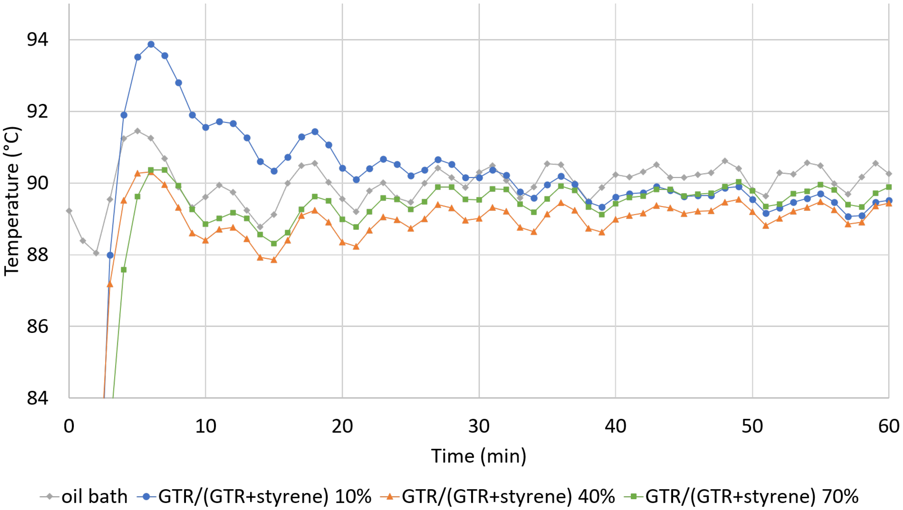
| T: | 90 °C | 100 °C | 110 °C | ||||||
|---|---|---|---|---|---|---|---|---|---|
| GTR/(GTR + Styrene): | 10% | 40% | 70% | 10% | 40% | 70% | 10% | 40% | 70% |
| Mean T after 1 h 30 | 89 | 89 | 89 | 99 | 99 | 100 | 106 | 106 | 109 |
| Min T after 1 h 30 | 88 | 87 | 88 | 98 | 98 | 98 | 104 | 105 | 108 |
| Max T after 1 h 30 | 90 | 90 | 91 | 101 | 101 | 101 | 108 | 108 | 111 |
| t (min) to reach T ± 2 °C | 3 | 3 | 4 | 2 | 3 | 3 | 2 | - | 5 |
| ML Algorithm | HPs | Split 1 | Split 2 | Split 3 | Split 4 | Split 5 | Time (1 Split) |
|---|---|---|---|---|---|---|---|
| GB | n_estimators | 150 | 150 | 150 | 150 | 150 | 3.8 s |
| learning_rate | 0.1 | 0.1 | 0.1 | 0.1 | 0.1 | ||
| max_features | ‘log2’ | ‘log2’ | ‘log2’ | ‘log2’ | ‘log2’ | ||
| min_samples_leaf | 5 | 5 | 5 | 1 | 1 | ||
| subsample | 1 | 1 | 0.8 | 0.6 | 0.4 | ||
| RF | n_estimators | 50 | 150 | 150 | 50 | 50 | 1.2 s |
| max_features | ‘log2’ | ‘log2’ | ‘log2’ | ‘log2’ | ‘log2’ | ||
| max_samples | None | None | None | None | None | ||
| MLP | activation | ‘relu’ | ‘relu’ | ‘relu’ | ‘relu’ | ‘relu’ | 27.5 s |
| hidden_layer_sizes | (15, 10) | (50, 5) | (5, 5) | (5, 15) | (5, 25) | ||
| solver | ‘lbfgs’ | ‘lbfgs’ | ‘lbfgs’ | ‘lbfgs’ | ‘lbfgs’ | ||
| learning_rate_init | 0.001 | 0.001 | 0.001 | 0.001 | 0.001 | ||
| max_iter | 800 | 800 | 800 | 800 | 800 | ||
| SVR | kernel | ‘rbf’ | ‘rbf’ | ‘rbf’ | ‘rbf’ | ‘rbf’ | 0.7 s |
| C | 1 | 4 | 8 | 1 | 2 | ||
| epsilon | 0.01 | 0.01 | 0.01 | 0.01 | 0.01 |
Disclaimer/Publisher’s Note: The statements, opinions and data contained in all publications are solely those of the individual author(s) and contributor(s) and not of MDPI and/or the editor(s). MDPI and/or the editor(s) disclaim responsibility for any injury to people or property resulting from any ideas, methods, instructions or products referred to in the content. |
© 2023 by the authors. Licensee MDPI, Basel, Switzerland. This article is an open access article distributed under the terms and conditions of the Creative Commons Attribution (CC BY) license (https://creativecommons.org/licenses/by/4.0/).
Share and Cite
Trinh, C.; Hoppe, S.; Lainé, R.; Meimaroglou, D. A Comprehensive Study on the Styrene–GTR Radical Graft Polymerization: Combination of an Experimental Approach, on Different Scales, with Machine Learning Modeling. Macromol 2023, 3, 79-107. https://doi.org/10.3390/macromol3010007
Trinh C, Hoppe S, Lainé R, Meimaroglou D. A Comprehensive Study on the Styrene–GTR Radical Graft Polymerization: Combination of an Experimental Approach, on Different Scales, with Machine Learning Modeling. Macromol. 2023; 3(1):79-107. https://doi.org/10.3390/macromol3010007
Chicago/Turabian StyleTrinh, Cindy, Sandrine Hoppe, Richard Lainé, and Dimitrios Meimaroglou. 2023. "A Comprehensive Study on the Styrene–GTR Radical Graft Polymerization: Combination of an Experimental Approach, on Different Scales, with Machine Learning Modeling" Macromol 3, no. 1: 79-107. https://doi.org/10.3390/macromol3010007