
Power Laws Govern the Abundance Distribution of Birds by Rank


1
Department of Economics, Federal University of Santa Catarina, Florianopolis 88049-970, SC, Brazil
2
Department of Statistics, University of Brasilia, Brasilia 70910-900, DF, Brazil
*
Author to whom correspondence should be addressed.
Birds 2023, 4(2), 171-178; https://doi.org/10.3390/birds4020014
Submission received: 28 October 2022
/
Revised: 29 March 2023
/
Accepted: 3 April 2023
/
Published: 7 April 2023
(This article belongs to the Special Issue Feature Papers of Birds 2022–2023)
Abstract
:Simple Summary
There are a lot of only a few kinds of birds. Scientists want to describe this fact with the right statistical distribution. Most of the time, the lognormal distribution is used. A new study, however, finds that the number of bird species is best described by a log left-skewed distribution. For the same set of data, we examine the rank abundance distribution rather than the species abundance distribution. In this case, the number of birds in each rank is based on a power law distribution.
Abstract
Only a few bird species are abundant. Understanding the abundance distribution of bird species is critical for conservation efforts because rare species may be more vulnerable to habitat loss, climate change, and other threats. According to new data, a log left-skewed distribution, rather than a lognormal distribution, better adjusts to the abundance distribution of bird species. We look at the rank abundance distribution rather than the species abundance distribution that use the same data and find three power laws: for the top four species; for the abundant species minus the top four; and for the rare species.
1. Introduction
Ecologists have long been interested in the distribution of the number of species occupying different numbers of sites independent of their abundance [1,2,3,4,5,6,7]. One of the few universal patterns in ecology is the distribution of species abundance [8]. The fact that some species are common but many more are rare is a crucial aspect of life’s diversity [9]. The lognormal distribution is widely accepted in the ecology literature for the distribution of species abundance [10]. A lognormal distribution emerges when the number of individuals or another measure of abundance is plotted on a log scale, usually of base 2.
Callaghan et al. [11] used the most recent influx of citizen science data to estimate the number of individuals (abundance) for 9700 bird species, accounting for roughly 92 percent of all birds. They merged counts from the app eBird (https://ebird.org/home, accessed on 27 October 2022), which allows users to record bird sightings, with data from 724 well-studied species. They then utilized an algorithm to extrapolate sample estimates. As a result, they discovered a large number of species with small populations confined in niche habitats, as well as a limited number of species spread throughout a large area.
Callaghan et al. [11] note that few of the species in their data are extremely abundant, and most have low population estimates. However, they also note that there would be about 200 more bird species than anticipated if the abundance of bird species followed a true lognormal distribution. They, therefore, propose a log left-skewed distribution.
A rank abundance curve (also known as a Whittaker plot) [12,13] is used by ecologists to show the relative abundance of species, which is a component of biodiversity. It can also be used to depict the richness and evenness of species [14]. The number of different species on the chart, or how many species were ranked, is referred to as species richness. The slope of the line that fits the graph indicates the number of species. When there is a steep gradient, the species at the top are more common than those at the bottom [14]. Because the abundances of different species are similar, a shallow gradient indicates high evenness. Estimates of bird species abundance are critical for ecology, evolutionary biology, and conservation, and progress in quantifying abundance is welcome. Rather than the distribution of bird species abundance, we are interested in the distribution of bird rank abundance using the same data as Callaghan et al. [11].
Instead of the lognormal and log left-skewed distributions, we use the Pareto distribution to model the bird rank abundance distribution. For the following reasons [15], the Pareto distribution may be a better choice for modeling than the lognormal and log left-skewed distributions: (1) Because the Pareto distribution has a long tail, it can better capture the presence of rare but abundant bird species. This is meaningful because, in ecological studies, rare species frequently have the greatest impact on the ecosystem; (2) The Pareto distribution has a simple parameterization that requires only two parameters (location and shape), making it easier to estimate and interpret than the lognormal and log left-skewed distributions, which frequently require more parameters; (3) The Pareto distribution is more robust to outliers than the lognormal and log left-skewed distributions, implying that it is less affected by extreme values in the data. This is important because ecological data frequently contains outliers, and the Pareto distribution can handle such situations better; (4) The Pareto distribution has a power-law behavior, which means it can capture the underlying mechanisms that generate bird species abundance patterns in an ecosystem; (5) When focusing on the tail of the data distribution, the Pareto distribution is more appropriate because the Pareto exponent is an index that describes the tail behavior, known as the Pareto tail index.
2. Materials and Methods
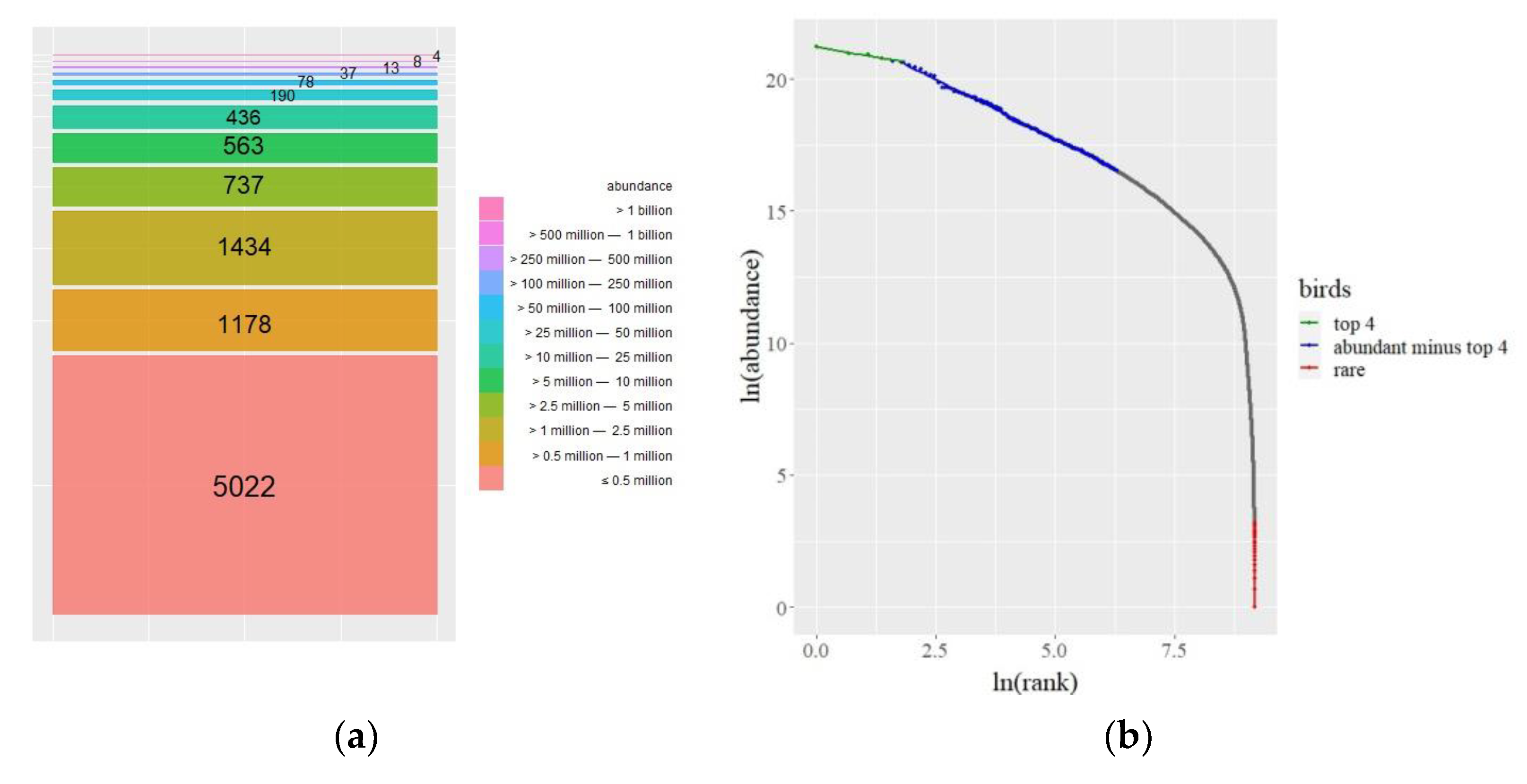
The data are depicted in Figure 1a. There are four undomesticated species with billions of individuals among the 50 billion birds: House Sparrows (Passer domesticus), European Starlings (Sturnus vulgaris), Ring-billed Gulls (Larus delawarensis), and Barn Swallows (Hirundo rustica). In comparison, each of the 5022 species has fewer than 500,000 birds. Figure 1a shows a glimpse of the power-law pattern we discover and immediately draws attention to the group of 1178 species that appear to deviate from the pattern, which we will discuss later.
A power law governs a quantity when the probability of receiving a given value varies inversely with its power [16]. Thus, a power law is a relationship between two quantities in which a change in one causes a proportional change in the other. This holds true regardless of the starting values. In the dynamics of hierarchical systems that arise in physics, economics, and biology, power laws are common. A power law appears geometrically as a straight line in a plot of the log of rank and the log of the quantity at hand. After ranking the bird species from top to bottom, three power laws emerge. Figure 1b is the result of plotting the log of rank against the log of bird abundance. The power laws in Figure 1b can be quantified by calculating their Pareto exponents in relation to the straight-line slopes.
One common approach is to use the survival function, , in a Pareto type I model [17]. Those bird species whose abundance exceeds x—that is, one minus the cumulative distribution function —are given by
where is the lower bound on abundance, and . The Pareto exponent (tail index) is the shape parameter that describes the heaviness of the right tail, with smaller values indicating a heavier tail.
We can estimate the three Pareto exponents associated with the rare and abundant species by ordinary least squares regressions of the log of the survivor function on the log of abundance and a constant term [17]. These result in straight-line intervals of slope (Figure 1b).
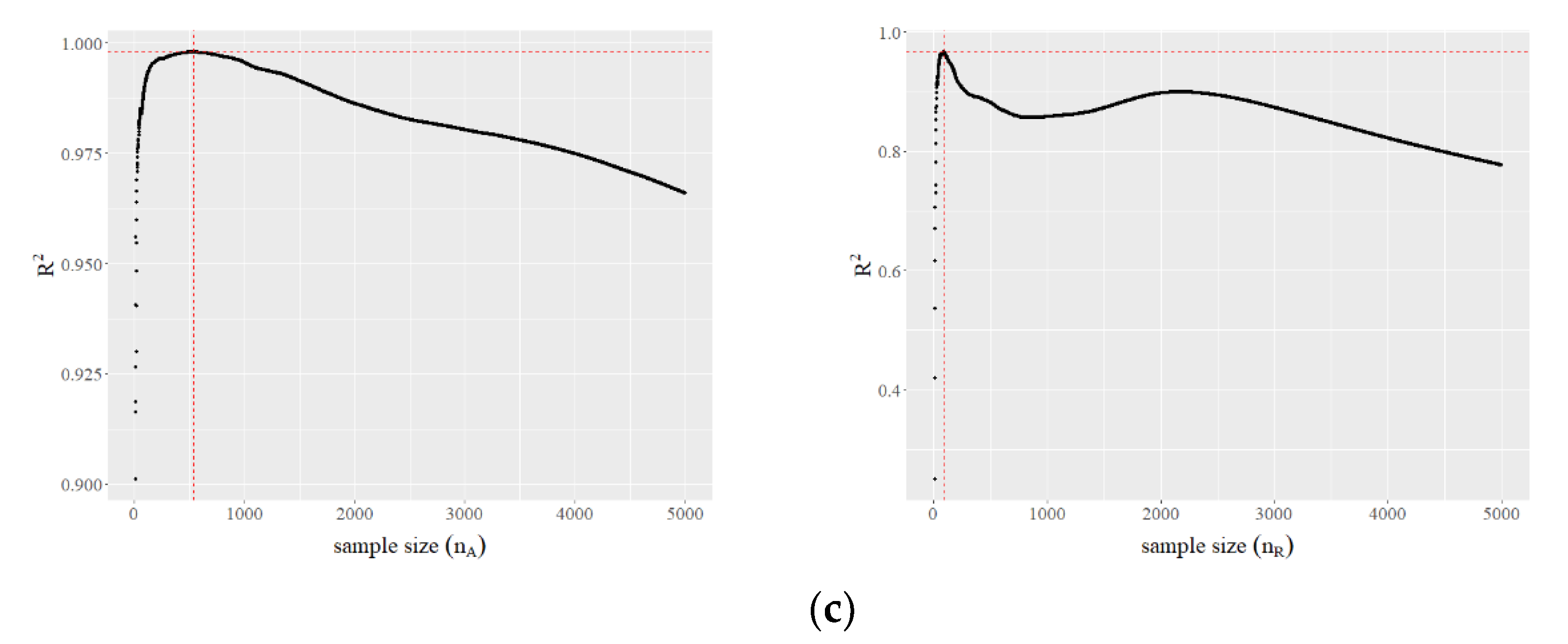
To determine the group of the most abundant species (aside from the top four), we run linear regressions varying from 10 to 5000 and record the corresponding values of the coefficient of determination . Then, we do the same for the rarer species, also ranging from 10 to 5000 (Figure 1c).
Our analysis focuses on the data distribution’s tail. The Pareto distribution is stable to truncations and, thus, is useful for studying tail behavior. To see how the Pareto distribution remains stable after a left truncation, consider a cutoff , such as in Equation (1). We can write the truncated distribution using the conditional distribution definition as
where This indicates that the truncated distribution follows a Pareto with the same index as the non-truncated Pareto.
3. Results and Discussion
For the most abundant species, model (1) fits well for the most abundant species, providing (p < ). As for the rarest species, the best fit presents (p < ) for the rarest species.
We compute the Pareto exponents for the three subsamples (Table 1). The value of is very close to zero for rare species, suggesting a heavier tail. Thus, these species are in a high uncertainty zone because there is no expected value for the number of rare species X. As a result, such species are in a non-equilibrium state, in which they can be on the verge of extinction (X = 0) or becoming increasingly rare. Apart from the top four, the distribution of the most abundant species has an expected value of X for abundance. The distribution, however, lacks a clear variability (as ), implying that this group is still vulnerable to abrupt hierarchical rank adjustments. Finally, the top four have the shortest tails.
The heaviness of the tail in the species rank abundance distribution reflects an ecosystem’s overall ecological stability and health, and can provide valuable insights into the dynamics of species coexistence and interactions [12]. Here are a couple of examples: (1) Endangered species are often scarce and have limited distributions. The heaviness of the tail in the species rank abundance distribution can indicate that many rare species are on the verge of extinction or have already gone extinct; (2) Rare species can have a significant impact on ecosystem functioning and stability. Rare plant species, for example, may have unique adaptations that allow them to survive in specific environmental conditions or provide habitat and food for specific wildlife species. The extinction of such rare species can have a domino effect on the rest of the ecosystem; (3) Rare species conservation is critical for preserving biodiversity and ecosystem resilience. The heaviness of the tail in the species rank abundance distribution may indicate that many rare species are at risk of extinction and require conservation attention; (4) The presence of many rare native species in the species rank abundance distribution may indicate that they are vulnerable to invasion and competition from non-native species.
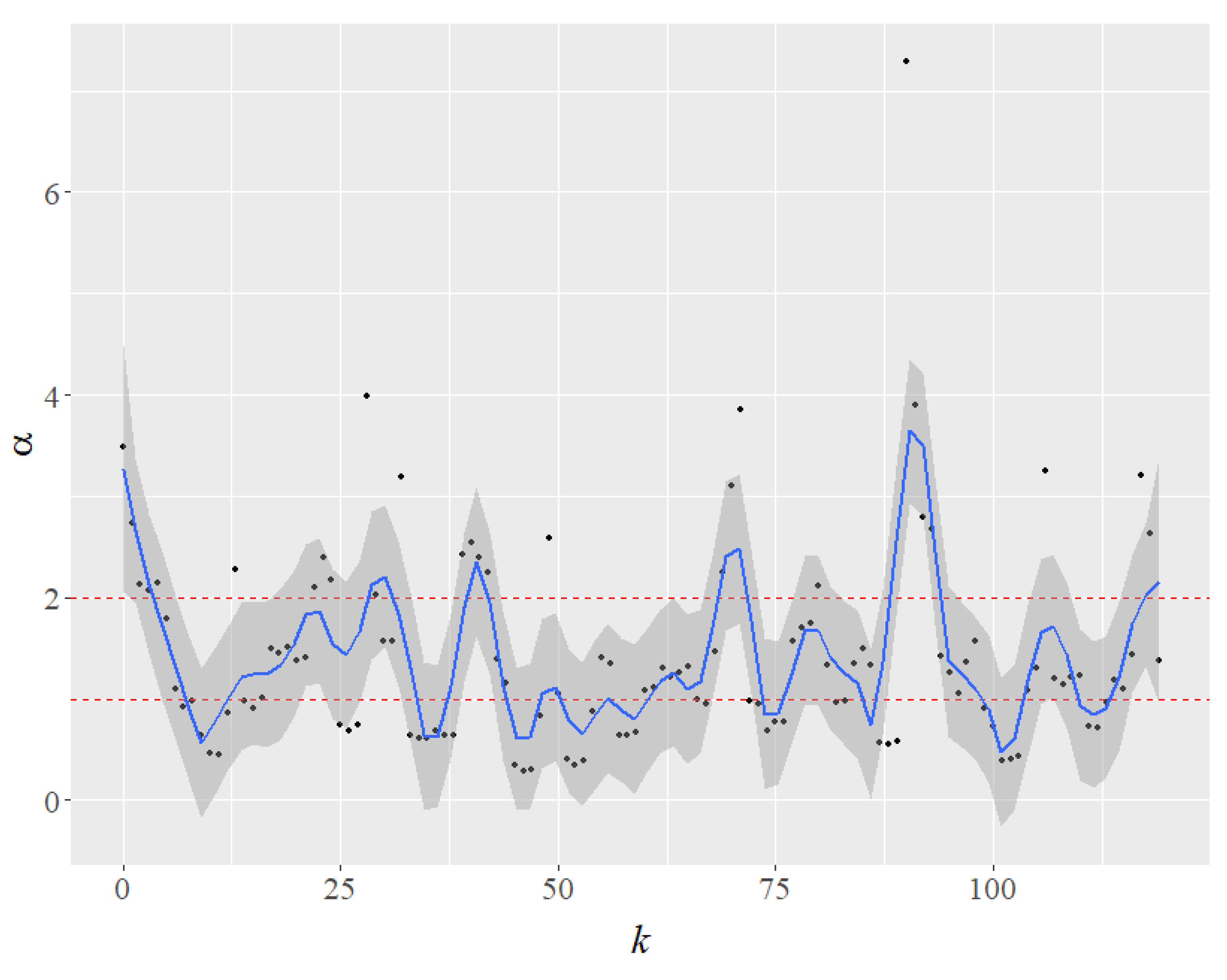
Our results are consistent with the literature, which shows that the risk of extinction varies across the avian phylogeny [18]. Consider a hypothetical evolution of the values of the Pareto exponent for the top four species as the k most abundant species are gradually removed (Figure 2). Because no abundant species are removed in the benchmark of Figure 1b, k = 0. The impact on the value of the Pareto exponent of removing the most abundant species is represented by k = 1, and the impact on the remaining top four is shown in Figure 2. The Pareto exponents are then computed after removing the two most abundant species (k = 2), the three most abundant (k = 3), and so on. In a Loess smooth curve fitting with a blue line (Figure 2), the shaded area represents a 95% confidence interval for . The results of the exercise show a pattern of interest in the impact of extinction on the remaining (top four) species. The Pareto exponents, in particular, become unstable. The alphas oscillate between light-tailed () and heavy-tailed regimes. Of note, when , the Pareto has no variance, and when , it has no mean either. As a result, the extinction of the big four significantly increases the overall uncertainty for the other species.
One could argue that more abundant species are less likely to become extinct than less abundant species. However, there are three major scenarios in which the extinction of the most abundant species is more likely than that of the less abundant species [12,19]: (1) More abundant species have larger ranges and may be more dependent on specific habitats. If their habitats are destroyed or altered, they may be unable to find suitable alternatives, resulting in population declines. The Monarch butterfly, for example, is a common species, but its numbers have declined due to the destruction of milkweed, the only plant on which Monarch caterpillars can feed; (2) More abundant species may be more appealing as hunting or fishing targets. Their populations can rapidly decline if they are overexploited. The Passenger Pigeon, for example, was once the most abundant bird in North America, but overhunting drove it to extinction in the early twentieth century; (3) Climate change can affect species in a variety of ways, but more abundant species are often more vulnerable to its effects. Corals, for example, are abundant in many reefs, but they are vulnerable to warming waters, ocean acidification, and other climate-related stresses, resulting in population and ecosystem declines. For the four most common bird species—House Sparrows, European Starlings, Ring-billed Gulls, and Barn Swallows—our hypothetical example may seem outlandish. The International Union for Conservation of Nature revises the conservation status of species every few years. Taking into account all relevant information, such as climate change, habitat degradation, and human factors, a panel of scientists currently classifies the conservation status of all of them as Least Concern, meaning that they are extremely unlikely to become extinct, barring unforeseen circumstances. Although this is the current consensus, we emphasize that the Pareto distribution’s ability to properly track outliers means that it also accounts for these “unforeseen circumstances”.
The abundance of species is shaped by a variety of ecological processes [20]. Many rarer species may have evolved to colonize a single island, for example, but human activity, such as deforestation, can also explain the pattern deviation in Figure 1a. Some species may be rare as a result of our interference. From the standpoint of conservation initiatives, this issue needs to be looked into further. Human activity, for example, is one of the most important factors explaining species richness in urban environments [21], and increasing urbanization has been shown to have a negative impact on bird species richness [22,23,24,25,26]. However, some species may benefit from urbanization and can be found in almost every town on the planet, while others may suffer, and still, others may neither benefit nor suffer [22]. Globally, urbanization causes taxonomic, functional, and evolutionary homogenization of urban animal and plant communities [27,28,29,30]. Rarer bird species were more often found in land-sparing urban areas than in land-sharing areas across Europe [26]. Because of urbanization, the winter bird community has a structure with few widely distributed sedentary core species and many partially migratory or migratory satellite species with a limited distribution [31].
A word of caution about the data is required here. Because bird enthusiasts tend to record bird sightings primarily in remote or urban areas where they live, the data may be biased. For example, if birders are more likely to observe and record birds in remote areas, urbanization may appear to have little effect on bird populations when, in fact, bird populations in urban areas may be declining. In contrast, if birders are more likely to observe and record birds in cities, urbanization may appear to have a greater impact on bird populations than it actually does.
4. Conclusions
Only a few bird species are abundant. Using new data, Callaghan et al. [11] propose that a log left-skewed distribution, rather than a lognormal distribution, adjusts better to the abundance distribution of bird species. Using the same data, we consider the rank abundance distribution rather than the species abundance distribution. Three different power laws are found: for the top four species; for the abundant species minus the top four; and for the rare species. Because power laws emerge even when data are scarce, our finding is not overly dependent on data quality.
The fact that many species, such as the third-most abundant Ring-billed Gull, have a Nearctic distribution among the top ten most abundant species may be one limitation of Callaghan et al.’s data. Because of this supposed limitation, the eBird database could not reliably estimate the abundance of most species that do not occur widely in the Americas. However, this criticism ignores the expert ornithologist knowledge that went into compiling the dataset, and we cannot know any better.
Our findings have important implications for bird community studies because they provide a more accurate picture of how bird populations are distributed in nature. This information can be used to guide conservation and management efforts. Understanding the power laws that govern the rank distribution of bird species, for example, can aid in forecasting how populations will respond to changes in their environment or management practices.
Author Contributions
Conceptualization, S.D.S. and R.M.; methodology, S.D.S. and R.M.; software, R.M.; validation, S.D.S. and R.M.; formal analysis, R.M.; investigation, S.D.S.; resources, R.M.; data curation, S.D.S.; writing—original draft preparation, S.D.S. and R.M.; writing—review and editing, S.D.S.; visualization, S.D.S. and R.M.; supervision, R.M.; project administration, S.D.S.; funding acquisition, S.D.S. and R.M. All authors have read and agreed to the published version of the manuscript.
Funding
This work is supported by the CNPq [Grant number: PQ 2 301523/2019 3]; Capes. [Grant number: PPG 001]: and FAP DF [Grant number: 1229/2016].
Institutional Review Board Statement
Not applicable.
Data Availability Statement
The data are available at https://www.ncbi.nlm.nih.gov/pmc/articles/PMC8166167/bin/pnas.2023170118.sd01.xlsx (Accessed on 27 October 2022).
Conflicts of Interest
The authors declare no conflict of interest. The funders had no role in the design of the study, in the collection, analyses, or interpretation of data, in the writing of the manuscript, or in the decision to publish the results.
References
- Hanski, I. Dynamics of regional distribution: The core and satellite species hypothesis. Oikos 1982, 38, 210–221. [Google Scholar] [CrossRef]
- Brown, J.H. On the relationship between abundance and distribution of species. Am. Nat. 1984, 124, 255–279. [Google Scholar] [CrossRef]
- Collins, S.L.; Glenn, S.M. Importance of spatial and temporal dynamics in species regional abundance and distribution. Ecology 1991, 72, 654–664. [Google Scholar] [CrossRef]
- Gilpin, M.E.; Hanski, I.A. Metapopulation Dynamics: Empirical and Theoretical Investigations; Academic Press: London, UK, 1991. [Google Scholar]
- McGeoch, M.A.; Gaston, K.J. Occupancy frequency distributions: Patterns, artefacts and mechanisms. Biol. Rev. 2002, 77, 311–331. [Google Scholar] [CrossRef]
- Jenkins, D.G. Ranked species occupancy curves reveal common patterns among diverse metacommunities. Glob. Ecol. Biogeogr. 2011, 20, 486–497. [Google Scholar] [CrossRef]
- Jokimaki, J.; Suhonen, J.; Kaisanlahti-Jokimäki, M.L. Urbanization and species occupancy frequency distribution patterns in core zone areas of European towns. Eur. J. Ecol. 2016, 2, 23–43. [Google Scholar] [CrossRef] [Green Version]
- Morlon, H.; White, E.P.; Etienne, R.S.; Green, J.L.; Ostling, A.; Alonso, D.; Enquist, B.J.; He, F.; Hurlbert, A.; Magurran, A.E.; et al. Taking species abundance distributions beyond individuals. Ecol. Lett. 2009, 12, 488–501. [Google Scholar] [CrossRef] [Green Version]
- Enquist, B.J.; Feng, X.; Boyle, B.; Maitner, B.; Newman, E.A.; Jorgensen, P.M.; Roehrdanz, P.R.; Thiers, B.M.; Burger, J.R.; Corlett, R.T.; et al. The commonness of rarity: Global and future distribution of rarity across land plants. Sci. Adv. 2019, 5, eaaz0414. [Google Scholar] [CrossRef] [Green Version]
- Chisholm, R.A. Sampling species abundance distributions: Resolving the veil-line debate. J. Theor. Biol. 2007, 247, 600–607. [Google Scholar] [CrossRef]
- Callaghan, C.T.; Nakagawa, S.; Cornwell, W.K. Global abundance estimates for 9700 bird species. Proc. Natl. Acad. Sci. USA 2021, 118, e2023170118. [Google Scholar] [CrossRef]
- Magurran, A.E. Measuring Biological Diversity; Blackwell: Oxford, UK, 2004. [Google Scholar]
- Whittaker, R.H. Dominance and diversity in land plant communities: Numerical relations of species express the importance of competition in community function and evolution. Science 1965, 147, 250–260. [Google Scholar] [CrossRef]
- Zhang, W.; Li, J.; Zhai, D.; Chen, Y.; Li, X.; Xu, H. A new method for measuring evenness of community composition. Ecol. Indic. 2019, 104, 509–516. [Google Scholar]
- Clauset, A.; Shalizi, C.R.; Newman, M.E. Power-law distributions in empirical data. SIAM Rev. 2009, 51, 661–703. [Google Scholar] [CrossRef] [Green Version]
- Newman, M.E. Power laws, Pareto distributions and Zipf’s law. Contemp. Phys. 2005, 46, 323–351. [Google Scholar] [CrossRef] [Green Version]
- Jenkins, S.P. Pareto models, top incomes and recent trends in UK income inequality. Economica 2017, 84, 261–289. [Google Scholar] [CrossRef] [Green Version]
- Purvis, A. Phylogenetic approaches to the study of extinction. Annu. Rev. Ecol. Evol. Syst. 2008, 39, 301–319. [Google Scholar] [CrossRef]
- Solow, A.R. Inferring extinction from sighting data. Ecology 1993, 74, 962–964. [Google Scholar] [CrossRef]
- McGill, B.J.; Etienne, R.S.; Gray, J.S.; Alonso, D.; Anderson, M.J.; Benecha, H.K.; Dornelas, M.; Enquist, B.J.; Green, J.L.; He, F.; et al. Species abundance distributions: Moving beyond single prediction theories to integration within an ecological framework. Ecol. Lett. 2007, 10, 995–1015. [Google Scholar] [CrossRef]
- Schlesinger, M.D.; Manley, P.N.; Holyoak, M. Distinguishing stressors acting on land bird communities in an urbanizing environment. Ecology 2008, 89, 2302–2314. [Google Scholar] [CrossRef]
- Blair, R.B. Land use and avian species diversity along an urban gradient. Ecol. Appl. 1996, 6, 506–519. [Google Scholar] [CrossRef]
- Marzluff, J.M. Worldwide urbanization and its effects on birds. In Avian Ecology and Conservation is an Urbanizing World; Marzluff, J.M., Bowman, J.M., Donell, M., Eds.; Kluwer Academic Press: Boston, MA, USA, 2001; pp. 1–17. [Google Scholar]
- Chace, J.F.; Walsh, J.J. Urban effects on native avifauna: A review. Landsc. Urban Plan. 2006, 7, 46–69. [Google Scholar] [CrossRef]
- Ortega-Álvarez, R.; McGregor-Fors, I. Living in the big city: Effects of urban land-use on bird community structure, diversity, and composition. Landsc. Urban Plan. 2009, 90, 189–195. [Google Scholar] [CrossRef]
- Suhonen, J.; Jokimäki, J.; Kaisanlahti-Jokimäki, M.L.; Morelli, F.; Benedetti, Y.; Rubio, E.; Pérez-Contreras, T.; Sprau, P.; Tryjanowski, P.; Møller, A.P.; et al. Occupancy-frequency distribution of birds in land-sharing and -sparing urban landscapes in Europe. Landsc. Urban Plan. 2022, 226, 104463. [Google Scholar] [CrossRef]
- Devictor, V.; Julliard, R.; Couvet, D.; Lee, A.; Jiguet, F. Functional homogenization effect of urbanization on bird communities. Conserv. Biol. 2007, 21, 741–751. [Google Scholar] [CrossRef]
- Ibanez-Alamo, J.; Rubio, E.; Benedetti, Y.; Morelli, F. Global loss of avian evolutionary uniqueness in urban areas. Glob. Chang. Biol. 2017, 23, 2990–2998. [Google Scholar] [CrossRef] [Green Version]
- McKinney, M.L. Urbanization as a major cause of biotic homogenization. Biol. Conserv. 2006, 127, 247–260. [Google Scholar] [CrossRef]
- Morelli, F.; Benedetti, Y.; Ibanez-Alamo, J.D.; Jokimäki, J.; Mand, R.; Tryjanowski, P.; Møller, A.P. Evidence of evolutionary homogenization of bird communities in urban environments across Europe. Glob. Ecol. Biogeogr. 2016, 25, 1284–1293. [Google Scholar] [CrossRef]
- Suhonen, J.; Jokimäki, J. Temporally stable species occupancy frequency distribution and abundance-occupancy relationship patterns in urban wintering bird assemblages. Front. Ecol. Evol. 2019, 7, 129. [Google Scholar] [CrossRef] [Green Version]
Figure 1.
(a) Only a few bird species are abundant (the numbers inside the bars represent the number of species). (b) Three power laws emerge when we take ln(rank) versus ln(abundance). (c) values versus sample size for the most abundant species (apart from the top four). The crossing of the dotted lines indicates the optimal sample size that provides a maximum (left). values versus sample size for the rarer species; the optimal sample size is with a maximum (right).


Figure 2.
Changes in the value of the Pareto exponent () as we simulate the impact of the extinction of the most abundant species (as k increases) on the other remaining four large species. The shaded area represents a 95% confidence interval for . When , the red dot lines represent light-tailed regimes; when , the Pareto distribution has no mean.


Table 1.
Finding the Pareto exponents.
| Group | Number of Species | Pareto Exponent | ||
|---|---|---|---|---|
| Top four | 4 | 0.972 | 3.485 (±0.422) ‡ | 73.90 (±8.85) ‡ |
| Abundant minus top four | 546 | 0.998 | 1.107 (±0.002) † | 24.62 (±0.04) † |
| Rare | 89 | 0.966 | 0.0027 (±0.00005) † | 9.18 (±0.0001) † |
† p-value < ; ‡ p-value <
Disclaimer/Publisher’s Note: The statements, opinions and data contained in all publications are solely those of the individual author(s) and contributor(s) and not of MDPI and/or the editor(s). MDPI and/or the editor(s) disclaim responsibility for any injury to people or property resulting from any ideas, methods, instructions or products referred to in the content. |
© 2023 by the authors. Licensee MDPI, Basel, Switzerland. This article is an open access article distributed under the terms and conditions of the Creative Commons Attribution (CC BY) license (https://creativecommons.org/licenses/by/4.0/).
Share and Cite
MDPI and ACS Style
Da Silva, S.; Matsushita, R. Power Laws Govern the Abundance Distribution of Birds by Rank. Birds 2023, 4, 171-178. https://doi.org/10.3390/birds4020014
AMA Style
Da Silva S, Matsushita R. Power Laws Govern the Abundance Distribution of Birds by Rank. Birds. 2023; 4(2):171-178. https://doi.org/10.3390/birds4020014
Chicago/Turabian StyleDa Silva, Sergio, and Raul Matsushita. 2023. "Power Laws Govern the Abundance Distribution of Birds by Rank" Birds 4, no. 2: 171-178. https://doi.org/10.3390/birds4020014