An Investigation into the Volumetric Flow Rate Requirement of Hydrogen Transportation in Existing Natural Gas Pipelines and Its Safety Implications

Abstract

As an alternative to the construction of new infrastructure, repurposing existing natural gas pipelines for hydrogen transportation has been identified as a low-cost strategy for substituting natural gas with hydrogen in the wake of the energy transition. In line with that, a 342 km, 36″ natural gas pipeline was used in this study to simulate some technical implications of delivering the same amount of energy with different blends of natural gas and hydrogen, and with 100% hydrogen. Preliminary findings from the study confirmed that a three-fold increase in volumetric flow rate would be required of hydrogen to deliver an equivalent amount of energy as natural gas. The effects of flowing hydrogen at this rate in an existing natural gas pipeline on two flow parameters (the compressibility factor and the velocity gradient) which are crucial to the safety of the pipeline were investigated. The compressibility factor behaviour revealed the presence of a wide range of values as the proportions of hydrogen and natural gas in the blends changed, signifying disparate flow behaviours and consequent varying flow challenges. The velocity profiles showed that hydrogen can be transported in natural gas pipelines via blending with natural gas by up to 40% of hydrogen in the blend without exceeding the erosional velocity limits of the pipeline. However, when the proportion of hydrogen reached 60%, the erosional velocity limit was reached at 290 km, so that beyond this distance, the pipeline would be subject to internal erosion. The use of compressor stations was shown to be effective in remedying this challenge. This study provides more insights into the volumetric and safety considerations of adopting existing natural gas pipelines for the transportation of hydrogen and blends of hydrogen and natural gas.

1. Introduction

The role of hydrogen in the transition to a low carbon economy has continued to surface among stakeholders in the scientific and industrial communities. One of the major benefits of hydrogen fuel is its nearly zero-carbon footprint at the point of utilization [1]. It can, therefore, serve in lowering carbon emissions. Despite this benefit, the development and implementation of the transportation infrastructure have been identified as one of the main challenges in the pursuit of a low carbon economy, where hydrogen replaces natural gas [2]. Consequently, as part of their strategy to use hydrogen, stakeholders plan to gradually change the composition of their existing gas infrastructure by blending hydrogen and natural gas. For instance, the UK is targeting 20 to 30% blends of hydrogen and natural gas in the short term. In the mid and long term, up to 100% hydrogen is planned for transportation along high-pressure pipelines [3]. This has been considered the most economically viable option for long-distance hydrogen transportation [4]. There are, however, many challenges that have to be addressed in the quest to transport hydrogen through existing natural gas pipelines. This includes the satisfaction of end-users since hydrogen possesses a lower heating value than natural gas. In addition to that, hydrogen is more susceptible to leakage from gas pipelines and the pipes are more vulnerable to embrittlement when transporting hydrogen than they are with natural gas [4]. Nonetheless, one benefit of hydrogen is its higher compressibility characteristics. Relative to natural gas, this attribute could enable hydrogen delivery at lower pressures, hence, reducing the potential risk of embrittlement that is associated with high-pressure (HP) flow in pipes [5].

Therefore, in addition to the determination of the amount of hydrogen gas that would deliver equivalent energy contents as natural gas, accurate investigation of the effect of fluid and flow properties such as the compressibility factor, and velocity on the safe and efficient transportation of hydrogen and hydrogen blends is important as they influence gas flow in the pipelines [6]. Additionally important are the choice and design of compressor stations [4] and the quality of the gas delivered [7].

Table 1. Properties of natural gas and hydrogen at 100 bar and 303 K.

Property	Methane	Hydrogen
Molecular weight (g/mol)	$16.0425$	$2.0159$
Density (kg/m3)	$74.6208$	$8\times {10}^{-3}$
Specific gravity	$5.539\times {10}^{-1}$	$6.96\times {10}^{-2}$
Dynamic viscosity (Pa·s)	$1.3955\times {10}^{-5}$	$9.168\times {10}^{-6}$
Kinematic viscosity (m2/s)	$1.8702\times {10}^{-7}$	$1.15\times {10}^{-3}$
Gross heating value (MJ/m3)	$37.6315$	$12.0793$
Thermal conductivity(W/(m·K))	$4.48\times {10}^{-2}$	$1.561\times {10}^{-1}$

provides the physical properties of both methane and hydrogen, which are essential in understanding their transportation in HP gas pipelines.

Although it is common knowledge that the energy content of natural gas is roughly three times that of hydrogen, the implications of tripling the gas volumetric flow rate for the flow of hydrogen in existing natural gas infrastructure to achieve the same energy value as natural gas is yet to be well understood. Furthermore, the safety of the process requires more critical analysis because of the wide discrepancies in flow properties that the flow of the two fluids will have under the same flow conditions due to their differences in physical and chemical properties. Therefore, the decision to transport hydrogen in natural gas pipelines will require answers to questions such as (i) how do the lower density and higher compressibility characteristics of hydrogen, relative to natural gas, affect its flow and what changes would be required for the flow of natural gas and hydrogen blends and the flow of 100% hydrogen in infrastructures originally designed for natural gas flow? and (ii) what modifications would be required to prevent hydrogen embrittlement and seepage for hydrogen flow in gas pipelines?

This work attempts to answer some of these and similar questions through process simulation of the transportation of hydrogen in natural gas pipelines by (i) estimating the volumetric flow rate equivalent of hydrogen that will deliver the same amount of energy as natural gas; (ii) providing an understanding of the effect of blending hydrogen with natural gas for transportation in existing natural gas infrastructure on flow parameters like the compressibility and velocity; and (iii) highlighting the implications of accelerating the volumetric flow rate of hydrogen in natural gas pipelines to provide an equivalent amount of energy as natural gas.

2. Theory

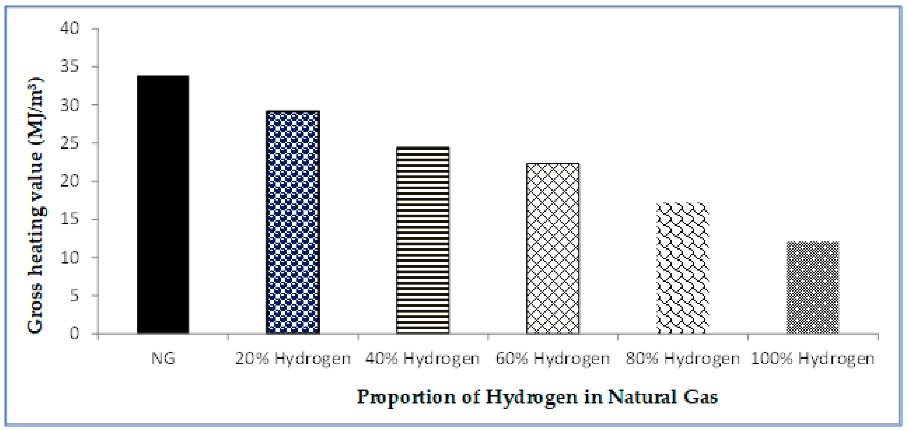
2.1. Energy Contents of Natural Gas and Hydrogen Blends

The energy or heating value of natural gas is reduced when it is blended with hydrogen. This property of natural gas-hydrogen blends has been attributed to the very low energy density of hydrogen [8]. In addition to the alteration in the energy value, blending natural gas with hydrogen significantly alters other combustion properties such as flame velocity, burning velocity, and greenhouse emissions [8,9,10]. Figure 1 shows the heating potential of various blends of methane/hydrogen mixtures.

2.2. Pipeline Transportation of Gases

Most of the industrial hydrogen is obtained from fossil fuels through steam reforming of natural gas and partial oxidation of methane. Natural gas is produced as associated gas from the gas cap of saturated oil reservoirs or solutions of undersaturated oil reservoirs and as non-associated gas from dry gas reservoirs [11,12]. These fossil fuels are rarely consumed or processed into finished products at their point of extraction.

While crude oil produced from land rigs can be stored on-site (in storage tanks) and later moved by land via tankers, rail, or transported through pipelines to refineries or sales terminals, crude oil from offshore platforms is seldom stocked on-site due to space constraints, but are usually transported through pipelines, for shallow waters, and through FPSO (Floating, Production, Storage, and Offloading) vessels for deep seas. Produced natural gas/methane, on the other hand, is transported almost immediately after they are produced and processed into pipeline quality gas through HP transmission pipelines or as LNG (liquefied natural gas), where pipeline transmission is geographically impossible or uneconomical [13]. Like natural gas, hydrogen gas often requires transportation from where it is manufactured to the locations of final consumption.

In the development of a hydrogen economy, the connection between locations where hydrogen is produced and where they are desired for use is a topic of great concern [14]. This has been adjudged by stakeholders to be less problematic and worrisome over short to medium distances, but challenging in long-distance pipelines [15]. Nonetheless, hydrogen has been transported safely with pipelines since the 1930s [14,16] and as of 2016, an estimated 4542 km of pipeline networks for hydrogen transportation existed globally with over 50% of them spread across the U.S. [17].

2.3. Hydrogen Pipelines: A Case for Adopting Existing Natural Gas Pipelines

Hydrogen has been adjudged to be a low-carbon fuel and acclaimed to possess the potential of being a major player in the energy transition toward global decarbonisation as a replacement for natural gas [18,19,20]. This presents the challenge of transporting it from the point of production to the location of end-users like most energy resources [15]. In the U.S. alone, for instance, existing natural gas infrastructure stretches up to three million miles of pipeline networks “including mainline and other pipes transport linking production and storage facilities with customers” [18]. Going by the American Petroleum Institute’s estimate of $5.34 million per mile for the cost of the average U.S. gas pipeline, using 30 inches for an average pipeline size [21], the cost of the three million miles of U.S. pipeline networks will amount to $16.02 trillion. To estimate an equivalent cost of hydrogen infrastructure, a multiplicative factor of 1.875 has been advised to account for the extra labour cost of the specialised sealing of pipe fittings (for hydrogen leakage prevention) and the cost of additional materials for the prevention of hydrogen embrittlement [22]. Therefore, an estimated $30.0375 trillion will be required to construct hydrogen infrastructure that will traverse the distance of today’s U.S. natural gas infrastructure. As an alternative to constructing new ones, adapting existing natural gas pipelines for hydrogen transportation could significantly reduce this cost.

The use of existing natural gas pipelines for hydrogen gas transportation has been given wide considerations in the past: pipeline transmission of hydrogen and natural gas blends has been rated as the most economical means of transporting large quantities of hydrogen over great distances [23]. Studies have also shown that if the hydrogen content of a hydrogen-natural gas mixture does not exceed one-fifth of the flow stream volume, it can be transported in existing natural gas pipeline networks with little or no modifications to the networks [15,24,25]. It has also been shown that 100% hydrogen can be transmitted at an approximately equal cost of 100% natural gas for a given distance of 500 km and an energy delivery rate of 1.0 GW if its production pressure is increased from atmospheric to a level of 6.5 bar, suggesting that long-distance transmission of hydrogen and hydrogen-methane blends may not be as economically viable as stakeholders posit [24]. In addition to these cost and technical implications, the introduction of hydrogen gas in existing natural gas infrastructure has more “energetic, material, and operational implications” that should be taken into cognisance, along with the effect of such practices on the performance of end-user equipment [25].

Some of the so-called “energetic” implications are the significant decrease in the volumetric flow rate (and total mass flow rates), the reduction in compressor power output, and increased energy consumption per compression stage per unit amount of delivered energy value and for a given set of operating conditions and pipeline dimensions that result when hydrogen is blended with natural gas and transported through pipelines because of the lower calorific value of hydrogen relative to natural gas or methane [15,23,25]; implying that the amount of energy delivered by the same pipeline will be a lot less with hydrogen and hydrogen-methane blends than it would be if it were to deliver only natural gas (methane) [26]. Quintino et al. [24] estimated that this loss could amount to about 10% in transport energy for a 100% shift toward a grid with 100% hydrogen.

The majority of concerns regarding the material implications of using an existing natural gas pipeline for hydrogen gas transportation centre on the safety implications such as the ability of hydrogen gas to embrittle materials, escape easily from containment, ignite under low amount of energy, its wide flammability range, and its extremely low density. It has been proven that the durability of some metal pipes can degrade when they are exposed to hydrogen over long periods, particularly with hydrogen in high concentrations and at high pressures [27]. To avoid embrittlement, it is advised that distribution lines, joints, and special parts are manufactured using steel containing a low percentage of carbon or tempered steels with tensile strength, $R_m<9500 \mathrm{bar}$, without superficial defects [15].

It is noteworthy, however, that studies on the “size of hazardous zones around pipelines transporting a mixture of natural gas and hydrogen indicate that, compared to pipelines transporting natural gas with the same parameters, the range of the zones is smaller” [23]. An estimate was also made of the drop in steel fracture toughness due to the impact of hydrogen. “The drop involves a rise in the probability of the pipeline damage. In the case of a gas mixture transport, the risk understood as the product of the probability of the gas pipeline failure and the effects thereof may be higher” [23].

In a nutshell, hydrogen gas transportation costs, like most commodities, are directly proportional to the distances to be covered whether they are transported with existing natural gas pipelines or not. Although additional expenditure would result from the modifications required to prevent hydrogen seepages and hydrogen embrittlement, as earlier mentioned, and also, an extra cost for the additional compression energy requirements per unit energy value, hydrogen transportation with the existing natural gas pipeline is a cheaper alternative to the creation of new hydrogen pipeline networks for the same purpose [23]. However, the cost of extracting hydrogen from the hydrogen and natural gas blend should be factored into the economic analysis of hydrogen transportation through existing gas infrastructure via blending with natural gas.

2.4. Flow Parameters in Hydrogen Pipelines

For minimum wall resistance to flow, even distribution of internal pressure, and minimal stagnation of the flow stream, gas transmission and distribution pipelines are cylindrical. Gas flow in circular pipes is governed by gas properties, operating conditions, pipeline properties, flow equations/gas laws/theories, and phenomena. Gas properties that are significant to gas flow in porous media and circular conduits like pipelines include gas composition, gas quality, apparent molecular weight ($M_a$), specific gravity (${\gamma }_g$), gas compressibility factor ($z$), gas density (${\rho }_g$), specific volume ($v$), isothermal gas compressibility coefficient ($c_g$), gas formation volume factor ($B_g$), gas expansion factor ($E_g$), and viscosity—dynamic, apparent, and kinematic [28,29]. Crucial operating conditions include pressure ($p$), temperature ($T$), Reynold’s number, flow rate, or velocity ($u$), etc. Pipeline properties relevant to gas flow include friction factor ($f$), pipe length ($L$), pipe diameter ($D$), etc., while the governing laws for gas flow in circular pipes include equations of state (EOS) like the General Gas law, Peng Robinson EOS, Pan Handle A. EOS, Virial EOS, etc., and the boundary layer theory [28,29]. The introduction of hydrogen into existing natural gas pipelines or blending of hydrogen with natural gas for transportation in existing gas networks will have effects on the above-mentioned flow behaviours, fluid properties, governing equations and laws. Such effects underscore the differences between hydrogen and natural gas transportation [30].

2.4.1. Hydrogen Blending Effect on Flow Parameters during Hydrogen Transportation in Existing Pipelines

Typical examples of the modifications to the properties and behaviour of the flow stream in existing gas pipelines that blending with hydrogen causes were observed in a recent study of the effects of hydrogen blending on the Joule–Thompson (J–T) coefficient of the flow stream when natural gas and hydrogen blends travel in pipelines [30]. In the work, the theoretical formulas for calculating the J–T coefficient of the natural gas-hydrogen mixture using the Soave–Redlich–Kwong (SRK) equation of state (EOS), Peng–Robinson EOS (PR–EOS), and Benedict–Webb–Rubin–Starling EOS (BWRS–EOS) were first derived and verified with empirical data. Then, the J–T coefficients of the flow stream at six different hydrogen blending ratios and thermodynamic conditions were calculated and analysed using the derived theoretical formulas and an already established empirical formula for calculating the J–T coefficient. It was discovered that the J–T coefficient of the natural gas-hydrogen mixture decreased approximately linearly with the increase in the hydrogen blending ratio such that when the hydrogen blending ratio reached 30% (mole fraction), the J–T coefficient of the natural gas-hydrogen mixture decreased by 40–50% compared to that of natural gas. This is significant because the J–T effect induces significant temperature changes, which can create extreme thermodynamic changes in the transportation network. For instance, its cooling effect can create conducive conditions for gas hydrate formation and consequent blockages in valves or gas pipelines and condensate banking/water drop out in the wellbore during wet gas, associated gas or condensate production. For the flow of hydrogen and natural gas blends, the J–T coefficient by the SRK–EOS, ${\mu }_{SRK}$, is expressed as shown in Equation (1) [30]:

$${\mu }_{SRK}=\frac{1}{c_p}\left[\frac{T}{{\rho }^2}{\left(\frac{\partial p}{\partial T}\right)}_{\rho ,PR}/{\left(\frac{\partial p}{\partial \rho }\right)}_{T,PR}-\frac{1}{\rho }\right]$$

(1)

where${\left(\frac{\partial p}{\partial T}\right)}_{\rho ,PR}=\frac{\rho R}{1-\rho b}-\frac{{\rho }^2\frac{da}{dT}}{1+\rho b}$; ${\left(\frac{\partial p}{\partial \rho }\right)}_{T,PR}=\frac{RT}{{\left(1-\rho b\right)}^2}-\frac{\left(2+\rho b\right)a}{{\left(1+\rho b\right)}^2}$; $\frac{da}{dT}=0.5{\displaystyle \sum }_{i=1}^C{\displaystyle \sum }_{j=1}^C{x}_i{x}_j\left(\frac{d{a}_i}{dT}{a}_i{}^{-0.5}{a}_j{}^{0.5}+a_i{}^{-0.5}{a}_j{}^{0.5}\frac{d{a}_j}{dT}\right)·\left(1-k_{ij}\right)$; $\rho =\frac{1}{v}$is the molar density in $\mathrm{kmol}/{\mathrm{m}}^3$; $a$ and $b$ are obtained from the SRK–EOS given in Equation (2) by mixing the corresponding coefficients of the components in the hydrogen and natural gas blend using the mixing rule given in Equation (3),

$$p=\frac{RT}{\left(v-b\right)}-\frac{a}{v\left(v+b\right)}$$

(2)

where $p$ is the system pressure, kPa; $T$ is the system temperature, K; $v$ is the molar volume${ \mathrm{m}}^3/\mathrm{kmol}$; $R$ is the universal gas constant, $R$ = 8.3145 $\mathrm{kJ}/\left(\mathrm{kmol}·\mathrm{K}\right)$; the attraction parameter $a=a\left(T_c\right)\alpha ,$ where $a\left(T_c\right)=\frac{0.42748R{T}_c^2}{P_c}$ and $\alpha ={\left[1+K\left(1-\sqrt{T_r }\right)\right]}^2$; $b=b\left(T_c\right)=\frac{0.008664R{T}_c}{P_c}$; $T_c$ and $P_c$ are critical temperature and critical pressure, respectively; $T_r$ is the reduced temperature, $T_r=\frac{T}{T_c}$; and κ = $0.48508+0.55171\mathsf{\omega } -0.15613{\mathsf{\omega }}^2$, where $\omega$is the acentric factor. The mixing rule used is:

$$a={\displaystyle \sum }_{i-1}^C{\displaystyle \sum }_{j=1}^C{y}_i{y}_j{\left(a_i{a}_j\right)}^{0.5}\left(1-k_{ij-SRK}\right), b={\displaystyle \sum }_{i=1}^C{y}_i{b}_i$$

(3)

where $C$is the total number of components; $y_i$is the mole fraction of component$i$; and $k_{ij-SRK}$ is the binary interaction coefficient between components$i$ and $j$ for the SRK–EOS, $k_{ij-SRK}=k_{ji-SRK}$, and$k_{ii-SRK}=0$.

Using the PR–EOS, the J–T coefficient for the flow of hydrogen and natural gas blends is expressed as shown in Equation (4) [30]:

$${\mu }_{PR}=\frac{1}{c_p}\left[\frac{T}{{\rho }^2}{\left(\frac{\partial p}{\partial T}\right)}_{\rho ,PR}/{\left(\frac{\partial p}{\partial \rho }\right)}_{T,PR}-\frac{1}{\rho }\right]$$

(4)

where ${\left(\frac{\partial p}{\partial T}\right)}_{\rho ,PR}=\frac{\rho R}{1-\rho b}-\frac{{\rho }^2\frac{da}{dT}}{1+2\rho b-{\rho }^2{b}^2}$; ${\left(\frac{\partial p}{\partial \rho }\right)}_{T,PR}=\frac{RT}{{\left(1-\rho b\right)}^2}-\frac{2\rho \left(1+\rho b\right)a}{{\left(1+2\rho b-{\rho }^2{b}^2\right)}^2}$; $\frac{da}{dT}=0.5{\displaystyle \sum }_{i=1}^C{\displaystyle \sum }_{j=1}^C{x}_i{x}_j\left(\frac{d{a}_i}{dT}{a}_i{}^{-0.5}{a}_j{}^{0.5}+a_i{}^{-0.5}{a}_j{}^{0.5}\frac{d{a}_j}{dT}\right)·\left(1-k_{ij}\right)$; $\rho =\frac{1}{v}$is the molar density in $\mathrm{kmol}/{\mathrm{m}}^3$; $a$ (the attraction parameter) and $b$ are obtained from the PR–EOS given in Equation (5) below by mixing the corresponding coefficients of the components in the hydrogen and natural gas blend using the mixing rule given in Equation (6),

$$p=\frac{RT}{\left(v-b\right)}-\frac{a}{v\left(v+b\right)+b\left(v-b\right)}$$

(5)

where$p$ is the system pressure, kPa; $T$ is the system temperature, K; $v$ is the molar volume${ \mathrm{m}}^3/\mathrm{kmol}$; $R$ is the universal gas constant, $R$ = 8.3145 $\mathrm{kJ}/\left(\mathrm{kmol}·\mathrm{K}\right)$; the attraction parameter $a=a\left(T_c\right)\alpha ,$ where $a\left(T_c\right)=\frac{0.457248R^2{T}_c^2}{P_c}$ and $\alpha ={\left[1+K\left(1-\sqrt{T_r }\right)\right]}^2$; $b=b\left(T_c\right)=\frac{0.00778T_c}{P_c}$; $T_c$ and $P_c$ are critical temperature and critical pressure, respectively; $T_r$ is the reduced temperature, $T_r=\frac{T}{T_c}$; and κ = $0.37464+1.54226\omega -0.26992{\omega }^2$, where $\omega ,$ the acentric factor is given by $w=\frac{3}{7}\left[\frac{{\log }_{10}\left(\raisebox{1ex}{$p_c$}\!\left/ \!\raisebox{-1ex}{$p_{atm}$}\right.\right)}{\raisebox{1ex}{$T_c$}\!\left/ \!\raisebox{-1ex}{$T_b-1$}\right.}\right]-1$; $T_b$ is the boiling temperature. The mixing rule used is:

$$a={\displaystyle \sum }_{i-1}^C{\displaystyle \sum }_{j=1}^C{y}_i{y}_j{\left(a_i{a}_j\right)}^{0.5}\left(1-k_{ij-PR}\right), b={\displaystyle \sum }_{i=1}^C{y}_i{b}_i$$

(6)

where $C$is the total number of components; $y_i$is the mole fraction of component $i$; and $k_{ij-PR}$ is the binary interaction coefficient between components$i$ and $j$ for the PR–EOS.

Similarly, the BWRS–EOS, the J–T coefficient for the flow of hydrogen and natural gas blends is expressed in Equation (7) [30] and like ${\mu }_{\mathit{SRK}}$ and ${\mu }_{\mathit{PR}}$, the values of ${\mu }_{BWRS}$, and its consequent cooling and/or heating effect on the flow of natural gas and hydrogen blends, will vary based on the proportions of hydrogen and natural gas in the blend.

$${\mu }_{BWRS}=\frac{1}{c_p}\left[\frac{T}{{\rho }^2}{\left(\frac{\partial p}{\partial T}\right)}_{\rho ,BWRS}/{\left(\frac{\partial p}{\partial \rho }\right)}_{T,BWRS}-\frac{1}{\rho }\right]$$

(7)

2.4.2. Gas Compressibility and Compressibility Factor Effects on Hydrogen Transport in Existing Gas Pipelines

Like the J–T coefficient discussed in the previous section, the gas compressibility factor is an important parameter in the flow of gases through pipes and porous media and its value will change significantly, relative to the value for the flow of natural gas, when blends of natural gas and hydrogen are being transported [10]. The compressibility factor is a measure of how much the behaviour of real gases deviates from the ideal gas law. The deviation exists because the ideal gas law (Equation (8)) was derived under the assumption that molecular volumes are not significant and that individual molecules do not possess attractive or repulsive forces between them; neither of which is true for real gases [28], especially at high pressures and low-temperature conditions. In other words, the compressibility factor tells us how much the thermodynamic properties of a real gas change from those expected from an ideal gas. It is determined by the gas composition [31] and can be expressed as the ratio of the actual volume of a real gas to the volume predicted by the ideal gas at the same temperature and pressure as the actual volume [32]. Therefore, the value of the compressibility factor for an ideal gas is unity (since there is no deviation in volume). “Air is very nearly an ideal gas where$z=1.0$. Methane and CO₂ exhibit distinctly nonlinear (and often nontrivial) response to applied force” [31]. The ideal gas law is defined as given in Equation (8):

$$pV=nRT$$

(8)

While the real gas law corrected for non-ideality is given by Equation (9):

$$pV=znRT$$

(9)

where $p$ = absolute pressure, $\mathrm{Pa}$; $V$ = volume, ${\mathrm{m}}^3$; $z$ = gas compressibility factor, $dimensionless$; $n$ = number of moles of the gas, $mole$; $R$ = universal gas constant, $8.314 \mathrm{J}/\mathrm{mol}·K$; $T$ = absolute temperature, $K$.

To reiterate the significance of the gas compressibility factor, it is worth mentioning that the negligence of the deviation from ideal gas behaviour is a leading cause of engineering failures in the oil and gas industry [31]. In addition, the compressibility factor is directly related to the density of a gas stream (Equation (9)), hence its flow rate and isothermal compressibility [29,31]. It is also an important tool for direct and indirect determination of many reservoir fluid properties in the oil and gas industry and a very essential variable for the quick estimation of the initial gas in place [12]. It is also an important factor to rely on when dealing with gas metering as the volume flow of gas obtained from the orifice meter depends on the accuracy of the z-factor [29]. Natural gas compressibility factor (z) is also a key factor in the gas industry for natural gas production and transportation [32,33] and can characterize the formation and behaviour of hydrates. Due to the aforementioned, several attempts have been made at estimating accurate values of the compressibility factor of gases and at understanding how they affect gas flow.

An early study undertaken to investigate the flow of gases in pipelines under scenarios of a constant gas compressibility factor throughout transient conditions and variable gas compressibility factors at a constant temperature defined by the pressure encountered during the transient flow revealed that compressibility factors change rapidly with varying pressure values [33]. This study, however, is limited by assumptions of negligible pipeline elevation changes, isothermal and single-phase flow, constant gas composition per experimental run, constant friction factors for a given pipe diameter, constant pipeline cross-sectional area, and the restriction of boundary conditions to only the inlet and outlet of the pipeline. Amongst others, the constant gas composition assumption precludes the findings of this work for use in the analysis of the compressibility behaviour of different proportions of natural gas and hydrogen blends.

Most recent works on the estimation of gas compressibility factors employed data science and artificial intelligence methodologies such as artificial neural networks and machine learning, which does not require the composition of the gas stream but properties such as the gas density, temperature, pressure and Joule–Thompson coefficients as input variables to study natural gas compressibility behaviours [34,35]. The results of such studies are, unfortunately, only as accurate as the number of data points used. Too few data points lead to model underfitting, while model overfitting and computational-intensiveness characterise too many data points. In addition, hydrogen transportation via existing natural gas pipelines has neither matured nor existed long enough to provide sufficient data points—say 30,000 [34]—for building machine learning models for the study of the compressibility behaviours of blends of natural gas and hydrogen in pipelines.

Empirical approaches have also been employed in the estimation of the compressibility factor and determination of gas compressibility behaviour. In another recent study, a high pressure (HP) pressure-volume-temperature (PVT) apparatus was used to determine the compressibility factors of samples of dry and wet natural gases from high temperature (HT) and ultra-high pressure oilfields in north-western China [36]. The authors discovered that the compressibility factors of these gas samples were considerably higher than those of conventional natural gases and a positive correlation was observed between the compressibility factor and the pressure within the high-pressure range investigated. Although the results of this work were found to be more accurate than estimates from five other established correlations for calculating the compressibility factor of natural gas, the study is grossly limited in the scope of applicability because the findings and methodology were not only confined to HT and ultra-HP gas wells but also streamlined to the range of experimental values. While the study could prove to be invaluable in the development of HP and HT gas wells, it provides little or no insight into the compressibility behaviour of blends of natural gas and hydrogen when they flow in pipelines.

2.4.3. Embrittlement Concerns and How They Can Be Avoided in Hydrogen Pipelines

Hydrogen embrittlement of metallic pipelines has been tagged a “chief technical concern” in the pipeline transportation of hydrogen gas [37]. In particular, pipeline welds are susceptible to embrittlement due to the microstructure changes that can occur during the welding process [37]. Hydrogen embrittlement of metals has been described as a hydrogen-assisted degradation process, which occurs when a combination of metal hydrogenation (that occur simultaneously with corrosion) and working stresses facilitate the development of in-bulk damage at nanoscales and microscales [38]. Conventional approaches to the prevention of embrittlement in hydrogen pipelines, therefore, work by impeding steel hydrogenation or limiting hydrogen diffusion into the lattice of the pipeline material [17,39,40,41]. For instance, because steel pipelines become very susceptible to hydrogen embrittlement for hydrogen concentrations above 30%, it has been advised that distribution network sections that are made of cast iron and steel are replaced with polyethylene [23].

2.4.4. Hydrogen Blending Effect on Pressure Behaviour in Gas Pipeline Transport of Hydrogen

Pressure is the energy that causes and drives the flow of fluids in conduits. It is defined as the force per unit area and expressed in SI unit of Pascal (Pa) or Newton per square metres (N/m²). The pressure drops of gas flowing in a pipeline is a function of the rate of gas flow, internal pipe diameter, pipe length, gas temperature, gas properties, properties of the pipe wall, and initial properties of the gas as defined in Equation (9) [28]. Figure 2 shows that the highest flow rate, $Q$, is indicated by curve (d) which has the highest pressure drop. This is followed by curve (c), then (b), and subsequently, curve (a), which has no flow.

The presence of hydrogen in natural gas increases the pressure losses over the pipeline [42] and hydrogen requires about four times more energy to travel in pipelines relative to natural gas [5], necessitating hydrogen to be transmitted in pipelines at higher pressures than natural gas [26]. This implies that natural gas transmission networks that are desired for use in high-pressure hydrogen gas transmission will require a significant upgrade in their pressure ratings, especially when the hydrogen-methane ratio in the blend exceeds the 20% limit earlier acclaimed to warrant no modifications to the gas network.

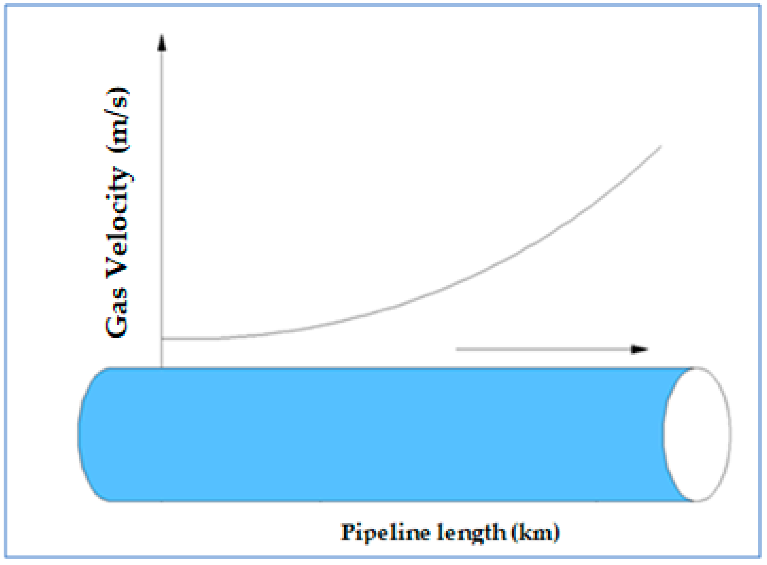
2.4.5. Hydrogen Blending Effect on Velocity during Hydrogen Transportation in Existing Gas Pipelines

The velocity of a flowing fluid stream is related to the volumetric flow rate$, Q\left(m^3/h\right)$, as shown in Equation (10).

$$Q=A\overline{v}$$

(10)

where $A$ is the cross-sectional area of flow, $m^2$ and $\overline{v}$ = velocity, $\raisebox{1ex}{$m$}\!\left/ \!\raisebox{-1ex}{$h$}\right.$.

The gas velocity in any transmission or distribution main can be mathematically expressed as given in Equation (11) and the maximum speed at which any gas can travel is limited to the speed at which sound can travel in the same gas [29]. However, natural gas cannot attain the speed of sound in methane (396 $\mathrm{m}/\mathrm{s}$) because natural gas typically flows at less than 20 $\mathrm{m}/\mathrm{s}$. This is considered the erosional velocity limit [29]. The behaviour of gas velocity profiles in natural gas pipelines is shown in Figure 3. The reason for this rise in velocity with increasing pipe length is explained in the next section.

Lighter components increase the velocity of a gas mixture in a horizontal pipe. However, the impact of density can overshadow the effect of the velocity of the mixture and result in increased pressure losses, even in inclined pipelines [42].

$$u=353.68p_s{\left[\frac{d}{d^5{p}_1{}^2-6211.1Q^{2}fSL}\right]}^{0.5}$$

(11)

where $u$ is the gas velocity, $m/h$; $p_s$ is the pressure at standard conditions, $Pa$; $p_1$ is the inlet pressure, $Pa$; $d$ is the pipe diameter, $m$; $Q$ is the volumetric flow rate, $m^3/h$; $f$ is the Fanning friction factor, $dimensionless$; $S$ is the specific gravity of gas, $dimensionless$; and $L$ is the pipe length, $m$.

2.4.6. The Concept of Erosional Velocity Limit

The fundamental principle of gas transportation as described by the boundary layer theory is that the collision of gas molecules with pipeline walls causes pressure losses due to friction, hence, gases continue to expand as the pressure drops across the length of the pipeline, causing an increase in the gas velocity. The huge difference in the density of natural gas versus hydrogen implies that hydrogen moves faster than natural gas in most cases along gas pipelines. Such an increase in velocity does not cause any safety concerns unless it reaches the erosional limit, above which its contact with the pipeline internal walls increases the pipe’s vulnerability to internal erosion and subsequent failure. For natural gas transmission pipelines, this limit is defined by Equations (11) or (12) [29,43,44].

$$v_e=N\frac{c}{\sqrt{\rho }}$$

(12)

where $v_e$is the erosional velocity ($\mathrm{m}/\mathrm{s}$); $N$is a constant that has a value of $1.22$ for converting Equation (12) from field units to metric units; the empirical constant, $c,$ranges in value from 100 to 250; and $\rho$ is the gas density ($\mathrm{kg}/{\mathrm{m}}^3$).

There is no theoretical velocity limit for gas flow in pipelines, however, a limit of 20 m/s is recommended to avoid internal erosion, which is aggravated by the presence of dust, which is a common occurrence, in gas pipelines [44].

2.5. Gas Network Modelling

Modelling and simulation of natural gas networks have enjoyed wide usage in recent times with many studies aiming to optimise different parameters ranging from a single objective such as the operating cost [45] to multiple operational objectives [46]. The inclusion of natural gas network models in power systems reliability studies has also been suggested by Munoz et al. [47] who explains that the methodology became expedient in the wake of increasing construction of combined-cycle power plants in which the gas and electricity systems are linked together for power generation in Spain and other countries. Like most of the cases reviewed below, the methodology employed in these gas network modelling studies are adequate and appropriate for the respective objectives of the studies, however, they have limitations such as constant gas composition assumptions (that limit them from being used in the modelling of hydrogen blending) and isothermal flow assumptions in the model development, which is rarely the case in real-life pipeline transportation of gases due to heat transfer between the gas stream and its environment and several temperature-altering thermodynamic changes that occur as the gas is transported, especially along long-distance transmission pipelines [48].

In the first case, Dorin and Leonida [49] developed a mathematical model for the modelling and simulation of natural gas flow in pipelines and analysed the necessary discretization processes needed for numeric integration of flow parameters such as pressure, temperature, and fluid properties. Furthermore, using an implicitly numeric integration method, more case studies of some flow processes through pipelines in distinct situations were developed. Results from the work were tested for their accuracy against the results of established empirical studies and deployed on the case studies. Despite the impressive performance of the model developed, as reported by the authors, it is limited by the assumption of isothermal conditions in the pipeline. Furthermore, the effect of the frictional loss during the pipeline transportation of natural gas was completely omitted from the model and elevation changes were either omitted or considered to be constant. These conditions are far from those of realistic natural gas transmission pipelines.

In a later, similar study, a more robust numerical model was developed that featured detailed representations of compressor stations for the simulation of pressure and other flow parameters of natural gas transmission pipeline networks of different configurations [50]. The flow parameters (or solutions of the model) were estimated using a visual C++ code developed based on the Newton–Raphson technique [51,52,53]. The model proposed in the study outperformed existing models for transmission pipeline network simulation in the estimation of the energy consumption for different configurations of natural gas transmission pipeline networks as model solutions (or flow parameters) were calculated with less than 10 iterations of the Newton–Raphson technique-based visual C++ code, thereby providing a tool for quick decision making and planning of natural gas transmission pipeline systems. In addition to the fundamental limitations of the Newton–Raphson solution techniques such as the low speed of convergence and the limited number of iterations [54,55], the model proposed in the study does not contain any constraint that restricts the estimated flow rate values to an erosional velocity limit (or alert operators when it is been approached) following the stipulation of API RP 14E [56]. Negligence for this safety concern could lead to internal erosions in the pipelines and consequent system failures.

Modelling of natural gas pipelines is not limited to long-distant pipeline transmission such as the scenarios discussed above. Studies of gas distribution network modelling and simulation have also been done and reported: in a study focusing on gas flow dynamics across gas ducts, two simplified models derived from the set of partial differential equations governing the dynamics of gas flow through ducts were presented [57]. The authors who recognised gas ducts as the main component in such kinds of networks accounted for pipeline inclination in the models, which were solved using two solution approaches that were implemented using the MATLAB-Simulink^® tool.

In a more recent gas distribution network modelling study that is more suitable for large-scale deployment, an integrated study was undertaken and outcomes of it were advised for use in assessing different strategies to improve the daily operation of the network. The study features a steady-state gas network model, a gas consumption model, sensor placement, leak detection, and leak minimization [58]. The gas network model was developed using the steady-state Weymouth equation. The recommendations of the work, though appropriately suited for natural gas distribution systems, are not suitable for use in the long-distance pipeline transmission of natural gas or natural gas and hydrogen blends as those were not in the scope of the study.

2.5.1. Capturing Individual Particle Interaction in Modelling of Gas and Hydrogen Blend Flow

In this work, it is crucial to understand the effects of the interactions of the molecules of the individual phases (natural gas and hydrogen) on the flow properties of the blends. Therefore, conscious efforts were made not to assume or utilise constant properties for our estimations where appropriate. For instance, although the SRK–EOS (Equation (2)) and PR–EOS (Equation (5)) are famous among petroleum and gas engineers for fluid flow and processes modelling, they are not ideal for the objectives of this study. This is because both of them assume a fixed value of the critical compressibility factor ($Z_c)$ “for all substances” including natural gas (“0.307 and 0.333 by PR and SRK respectively, whereas $Z_c$ varies within a range of 0.2 to 0.3 for hydrocarbons”) [59]. Therefore, a different and more appropriate model, the Esmaeilzadeh–Roshanfekr (ER–EOS) was used in this work. The ER–EOS [60] is a components–dependent cubic EOS that models the interactions between molecules using the principles of the generalized Van der Walls theory. The ER–EOS is presented in Equation (13):

$$P=\frac{RT}{v-b}-\frac{a\left(T\right)}{v\left(v+c\right)+c\left(v-c\right)}$$

(13)

where$\upsilon$ is the molar volume${ \mathrm{m}}^3/\mathrm{kmol}$; $R$ is the universal gas constant, $R$ = 8.3145 $\mathrm{kJ}/\left(\mathrm{kmol}·\mathrm{K}\right)$; $“a”$ is a function of temperature; and $“b”$ and$“c”$ are constants described as $\mathrm{a}\left(T_c\right)={\Omega }_a\frac{{\left(R{T}_c\right)}^2}{P_c}·\alpha \left(T_r\right);$ $b={\Omega }_b\frac{\left(R{T}_c\right)}{P_c}$ and; $c={\Omega }_c\frac{\left(R{T}_c\right)}{P_c}$. ${\Omega }_a=3{\varsigma }_c+{\Omega }_c{}^2++2{\Omega }_b{\Omega }_c+2{\Omega }_c$; ${\Omega }_b=2{\Omega }_c-1+3{\varsigma }_c$ and; ${\Omega }_c{}^3+\left(3{\varsigma }_c-\frac{5}{8}\right)·{\Omega }_c{}^2+\left(3{\varsigma }_c{}^2-\frac{3}{4}{\varsigma }_c\right)·{\Omega }_c+{\varsigma }_c{}^3-\frac{3}{8}{\varsigma }_c{}^2$; $\alpha \left(T_r\right)$ is obtainable from $\alpha ={\left[m_1+m_2\left(1-T_r^{0.5}\right)\right]}^2$, where$m_1$,$m_2$, and ${\varsigma }_c$ are three substance-dependent parameters that make the ER–EOS equation more suitable for modelling component interaction at the molecular level. It has also been rated as the most accurate for modelling the properties of light hydrocarbon phases such as gas condensates in pipe conduits relative to PR and EOS, which are more reliable for liquid hydrocarbons such as oil [60,61].

2.5.2. Pressure Gradient and Pressure Losses Modelling

A generic form of the pressure gradient for the flow of gas, liquid, or both phases in a pipe was presented by Beggs and Brill, as shown in Equation (4) [62]. This robust model, derived from laboratory data, applies to vertical, horizontal, uphill-inclined, and downhill-inclined flow of gas. It has therefore enjoyed wide application for pressure gradient modelling in petroleum and gas engineering processes. However, like most empirically derived models, the Beggs and Brill model was developed based on accurately and reliably measured flow parameters under laboratory conditions, so that it can only work best on the proposed data range [63].

$$\frac{-dp}{dZ}=\frac{\frac{g}{g_c}\sin \theta \left[{\rho }_L+{\rho }_g\left(1-H_L\right)\right]+\frac{f_{tp}{G}_m{v}_m}{2g_{c}d}}{1-\frac{\left[{\rho }_L{H}_L+{\rho }_g\left(1-H_L\right)\right]v_m{v}_{sg}}{g_{c}p}}$$

(14)

A major cause of pressure losses in pipes is the frictional drag exerted by the pipe walls on the moving fluid stream. This pressure loss, due to the wall friction, is expressed in terms of the friction factor of the fluid flow. It is related to the Reynolds number and relative roughness of the flow and pipe, respectively, as given by Colebrook and White [64] in Equation (5).

$$\frac{1}{\sqrt{f}}=-2{\log }_{10}\left(\frac{\epsilon }{3.7D}+\frac{2.51}{R_e\sqrt{f}}\right)$$

(15)

where $f$ stands for Darcy’s friction factor; $R_e$ is the Reynolds number; and $\epsilon /D$ is the relative roughness of the pipe. The variables $f$, $R_e$ and $\epsilon /D$ are all dimensionless.

3. Study Methodology

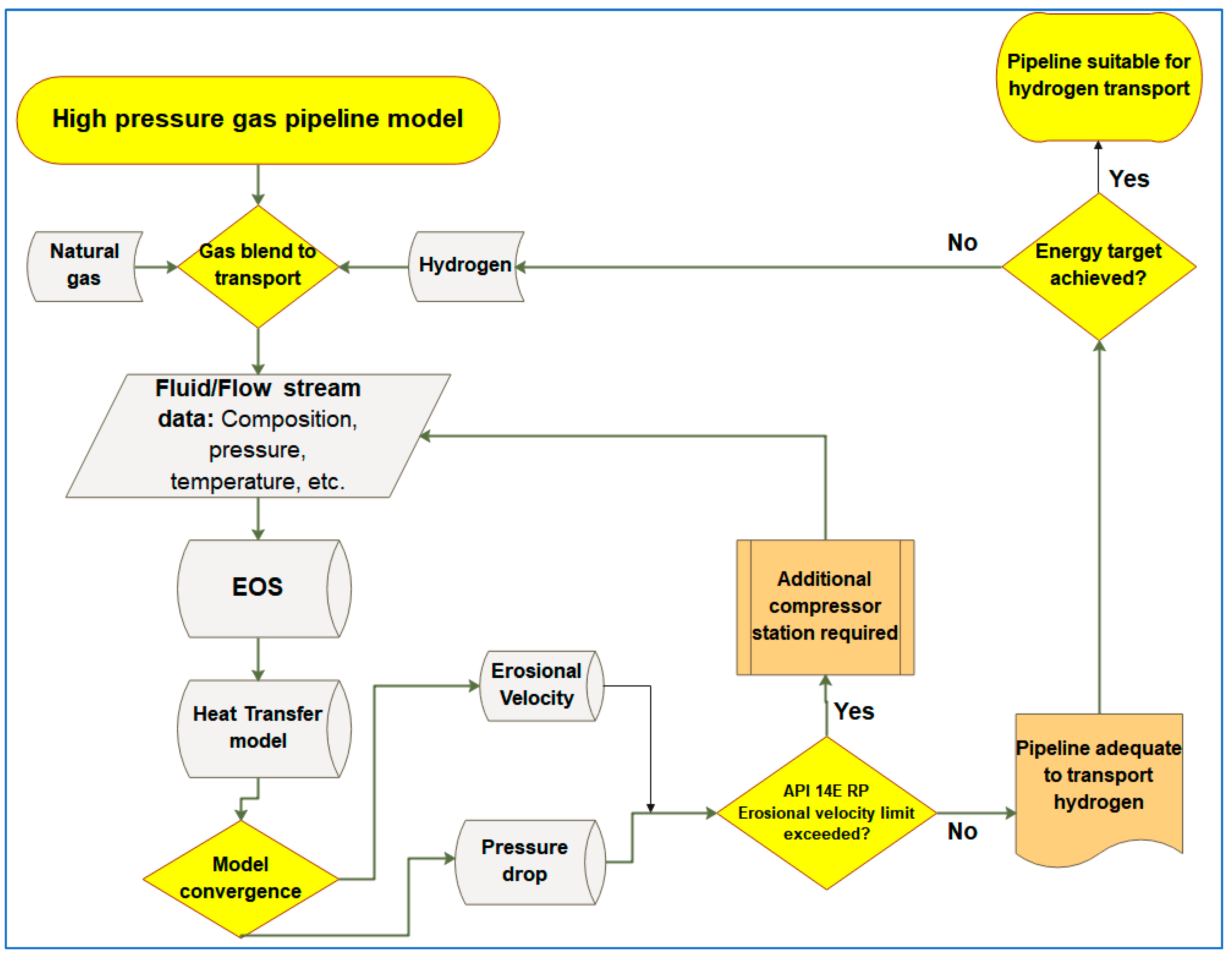
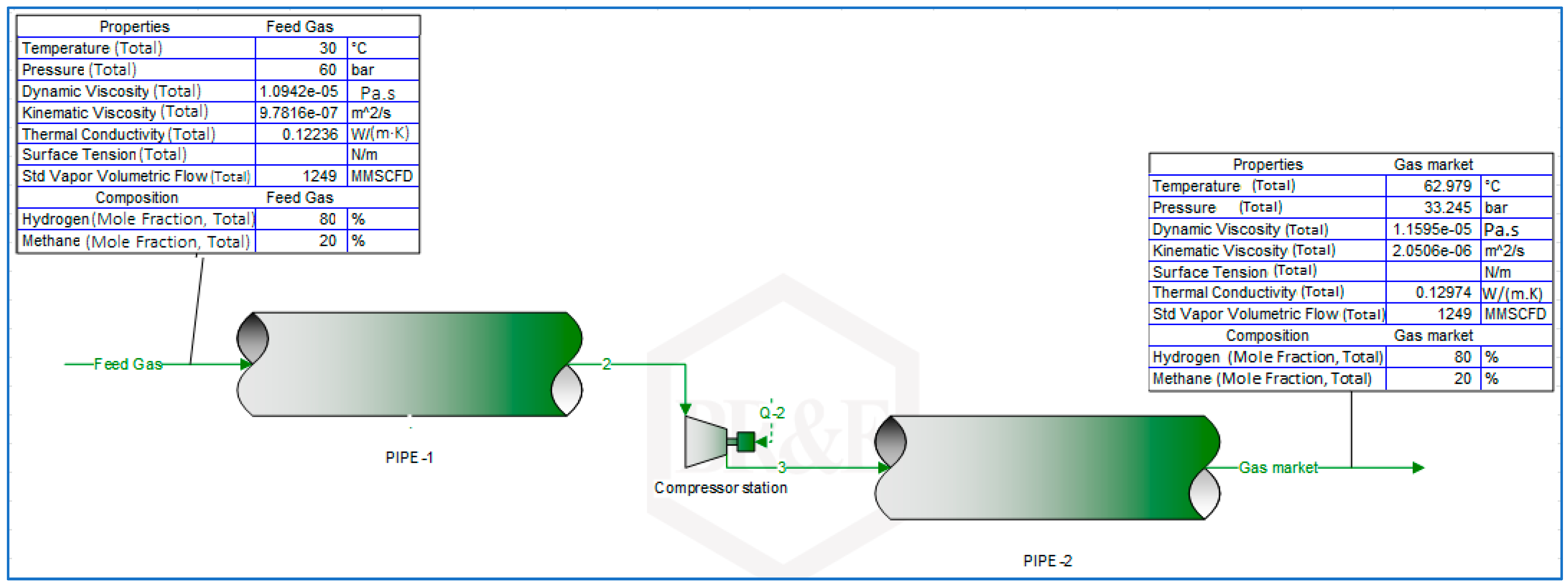
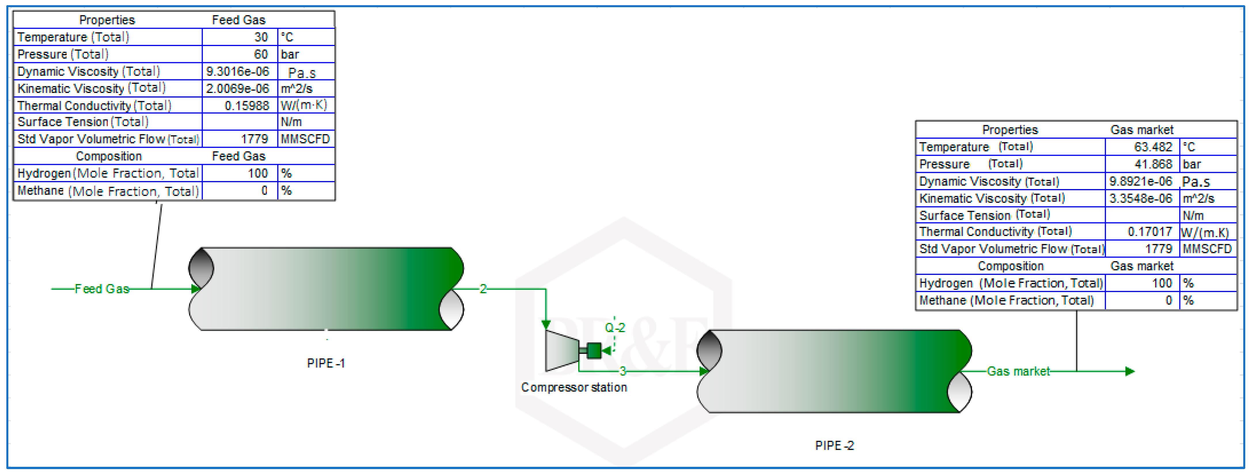
3.1. Simulation Workflow for the Transportation of Hydrogen and Natural Gas Blends in Existing Gas Pipelines

In this study, a generic high-pressure pipeline model of 60 bar inlet pressure, delivering to a power plant 342 km away was developed using a pipe diameter of 36″. The natural gas phase used throughout this work has the compositions specified in

Table 2. Components of the natural gas phase.

Component	Mole Fraction (%)
Methane	93.76
Ethane	3.14
Propane	0.62
Butane	0.2
Pentane	0.07
Nitrogen	2.03
Carbon Dioxide	0.18

and the gas network analysis tool used was the Promax^® Process Simulator. The generic experimental workflow is presented in Figure 4.

The Esmaeilzadeh–Roshanfekr Equation of States (ER–EOS) (Equation (13)) was utilized for the P–V–T–z (pressure–volume–temperature–composition) modelling in all the experiments. In addition to its suitability for modelling lighter hydrocarbons relative to the PR–EOS and the SRK–EOS [60,61], the choice of the ER–EOS is motivated by the objective of accurately capturing the individual property interactions of the two phases in the natural gas and hydrogen blends as opposed to modelling the flow stream as a single component.

The Beggs and Brill multiphase flow model [62] was used for the pressure gradient modelling throughout the study for its versatility and suitability for gas modelling.

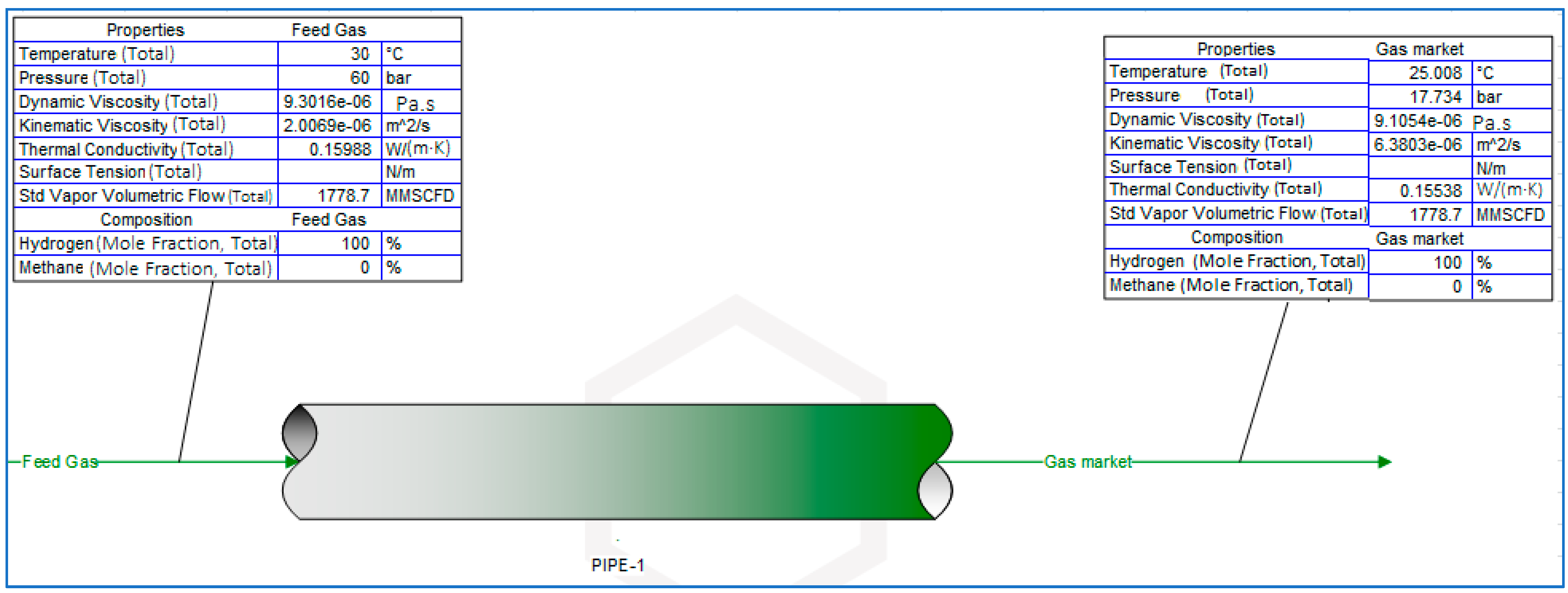
3.2. Determination of Volumetric Flowrate Requirements for Constant Energy Delivery by Hydrogen and Natural Gas Blends through Natural Gas Pipelines (Free-Flow Modelling)

To find the equivalent volumetric flow rate of hydrogen that will deliver the same amount of energy as a unit volumetric flow rate of natural gas, the pipeline model in Figure 5 was used. In addition to the inlet and outlet parameters and the flow stream compositions indicated in Figure 5 for 100% hydrogen, more attributes of the pipeline are presented in

Table 3. Additional model parameters for high-pressure flow of hydrogen in natural gas pipelines.

Input Variable	Value	Unit
Pipe length	342	km
Nominal pipe size, NPS	36	inch
Pipe wall thickness	0.25	inch
Maximum allowable operating pressure, MAOP (inlet)	70	bar (g)
Outlet pressure	17.34	bar (g)
Gas specific heat ratio	1.4	NA
Standard temperature	15.5	°C
Atmospheric pressure	1.01325	bar
Number of length of pipe increment	200	NA
The material of pipe construction	Carbon steel	NA
Inclination angle	0	degrees
Inlet pressure	60	bar (g)

and Intermediate blends with 20, 40, 60, and 80% hydrogen proportions were also investigated.

The simulation approach is shown in Figure 4 (without the use of compressor stations). The desired energy requirement was set at 6440 MW, while the fluid properties and pressure gradient calculations were obtained as described in Section 3.1. Results of the experiment are presented in Section 4.1.

3.3. Investigating Safety Concerns of Hydrogen Transportation in Gas Pipelines

Regarding concerns for the reliability of existing pipeline infrastructure in transporting hydrogen, another key issue that has attracted significant concern is the safety of the pipelines [65]. This section explores some safety concerns that can arise from adopting existing natural gas pipelines for hydrogen transportation via hydrogen and natural gas blending. Specifically, the effects of blending on compressibility and the velocity profile of the flow in the pipeline were explored.

3.3.1. Investigating Hydrogen Blending Effects on Compressibility Factor in HP Pipelines

The gas compressibility factor was shown in Section 2.4.2 to be both significantly dependent on other flow parameters such as temperature and composition and capable of influencing other crucial physical flow parameters such as the pressure—a prominent factor in high-pressure pipelines [36].

Considering that negligence of the deviation from ideal gas behaviour (or the compressibility factor) is a leading cause of engineering failures in the oil and gas industry [31], this section investigates the effect of blending on the compressibility factor of the flow stream in a gas pipeline. To do this, the HP gas pipeline model was built with the parameters in Table 3. Additionally, the fluid and multiphase flow correlations used for the free-flow modelling (Section 3.2) were retained. However, the proportions of hydrogen and natural gas were varied in increments of 10 from 100% natural gas flow stream to 100% hydrogen flow stream. Different flow scenarios were investigated by varying the pipeline pressure from 0 to 100 bar in increments of 20 bar. The flow pipeline velocity profile was monitored throughout the experiment to ensure compliance with the limits stipulated in international standard API 14E RP [56]. The compressibility factors exhibited the behaviour described in Section 4.2.1.

3.3.2. Investigating Hydrogen Blending Effect on Flow Velocity in HP Gas Pipelines

The concept of maximum erosional velocity and the significance of monitoring the velocity profile of the flow stream in a gas pipeline are elaborated in Section 2.4.6. In essence, the mixture velocity should be kept below the erosional velocity value obtained from Equation (12) or the recommended 20 m/s for natural gas pipelines [44]. In this section, the effect of hydrogen blending on the behaviour of the velocity of the flow stream was studied. To do this, the model and experimental procedure described above (Section 3.3.1) was used, but at a constant pressure of 60 bar and temperature of 303.15 K, and the flow velocity profile along the length of the pipeline was monitored and recorded (See Section 4.2.2).

3.4. Keeping Pipeline Velocity Profiles within Recommended Limits with the Use of Compressor Stations

In

Table 4. Erosional velocity range for pipeline flow of natural gas at 60 bar, 303.15 K.

$c$	100	125	150	175	200	225	250
$v_e$ (m/s)	18.149	22.687	27.224	31.761	36.299	40.836	45.374

, the erosional velocity values for different values of the constant,$c$, were estimated from Equation (12) for the flow of natural gas at 60 bar inlet pressure and 303.15 K. At these conditions, the mass density of the natural gas mixture used in this study was estimated (with the composition provided in Table 3) to be $45.185 \mathrm{kg}/{\mathrm{m}}^3$. The velocity profiles estimated from Section 3.3.2 for the flow of different blends of hydrogen were subsequently benchmarked against the estimates in Table 4 to assess the safety of transporting hydrogen and blends of hydrogen and natural gas in the natural gas pipeline. For some proportions of hydrogen in the blend, the pipeline velocity rose above both the recommended erosional limit of 20 m/s and even above the worst-case scenario of 45.374 m/s, as shown in Table 4 (Section 4.2.2). To ensure that the velocities in the pipeline remain below the erosional velocity limit throughout the network, a compressor station was utilized midway along the 342 km pipeline (Section 3.3.2). The modified model thus consists of two 171 km pipelines and a compressor station (as shown in Figure 6 and Figure 7) and was modelled for the flow conditions of 80% hydrogen/20% natural gas blend and 100% hydrogen, respectively.

The compressor defined in the model has a power of 27.507 MW, with a polytropic efficiency of 75%, and pressure change across the compressor station was set at 16 bar. The results of the experiments—the velocity profiles in the pipelines for different proportions of hydrogen and natural gas blends—are presented in Section 4.3.

4. Results Presentation and Analysis

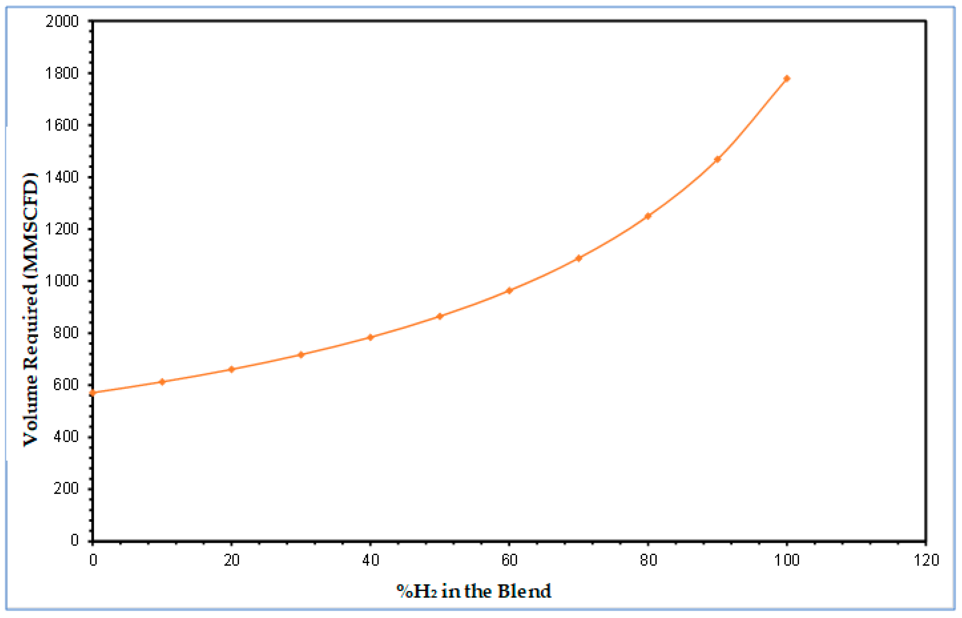
4.1. Constant Energy Delivery Volumetry Requirements of Transitioning from Natural Gas to Hydrogen

The current energy delivery dilemma around switching from natural gas to hydrogen is the volumetric inequalities imposed by the differences between natural gas and hydrogen. With hydrogen having lower energy contents (12 MJ/m³) compared to natural gas (36 MJ/m³), it is essential to understand that an equal volume of hydrogen transported in natural gas pipelines will only deliver about one-third of the total energy required. The energy content gap can be bridged using additional hydrogen injected into the pipeline, depending on the blend’s composition required. In this study, the equivalent volumetric flow rate required for the same volume of natural gas and different proportions of hydrogen and natural gas blends to deliver 6440 MW of energy were estimated and are shown in Figure 8.

From Figure 8, the equivalent volume of 100% hydrogen that would deliver the same 6440 MW supplied by 570 MMSCFD of natural gas is 1779 MMCSFD. Therefore, while discussions around smooth energy transition to hydrogen advocate for the adoption of existing pipeline infrastructure, it is noteworthy that to meet the volumetric equivalence of hydrogen in natural gas pipelines, the gas flow rate would need to be tripled for 100% hydrogen transport. Increasing the capacity of the pipeline by such a factor could trigger flow characteristics such as compressibility, velocity, and pressure drop to exceed the allowable safe limits stipulated by industry standards such as the API RP 14E, ASME B31.8, and BS 8010. In the subsequent sections, the effect of this volumetric constraint is investigated by exploring the relationship between the pressure, compressibility factor, velocity, and density of the blends under different flow conditions and compositions.

4.2. Investigating Safety Concerns in Transporting Hydrogen with Natural Gas Pipelines

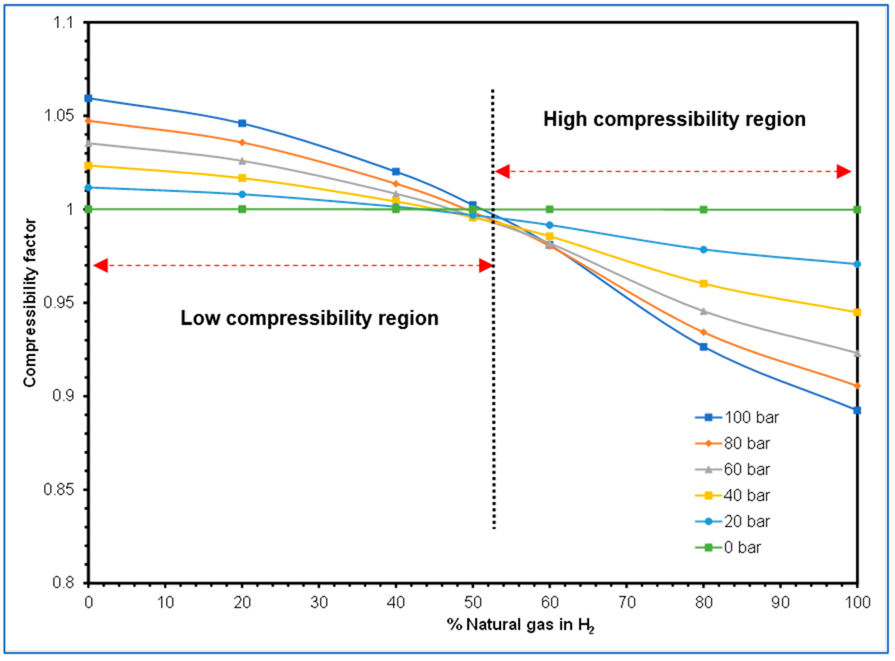
4.2.1. Hydrogen Blending Effect on Compressibility Factor along the High-Pressure Pipeline

The compressibility behaviour when the flow stream is a blend of natural gas and hydrogen revealed two signeted regions: one of low compressibility associated with high hydrogen content in the blend (up to 50–100%), and the region of high compressibility associated with high natural gas (principally, methane), as shown in Figure 9. An interesting observation in the behaviour of the compressibility factor is the wide range of values that can be exhibited by the flow stream. For instance, the 100 bar curve (Figure 9) showed extreme high and low compressibility values, which tended to flatten with a decrease in pressure. This is a significant indication that hydrogen transportation through pressure pipelines could be challenging due to the dynamic nature of the flow stream compressibility at HP conditions.

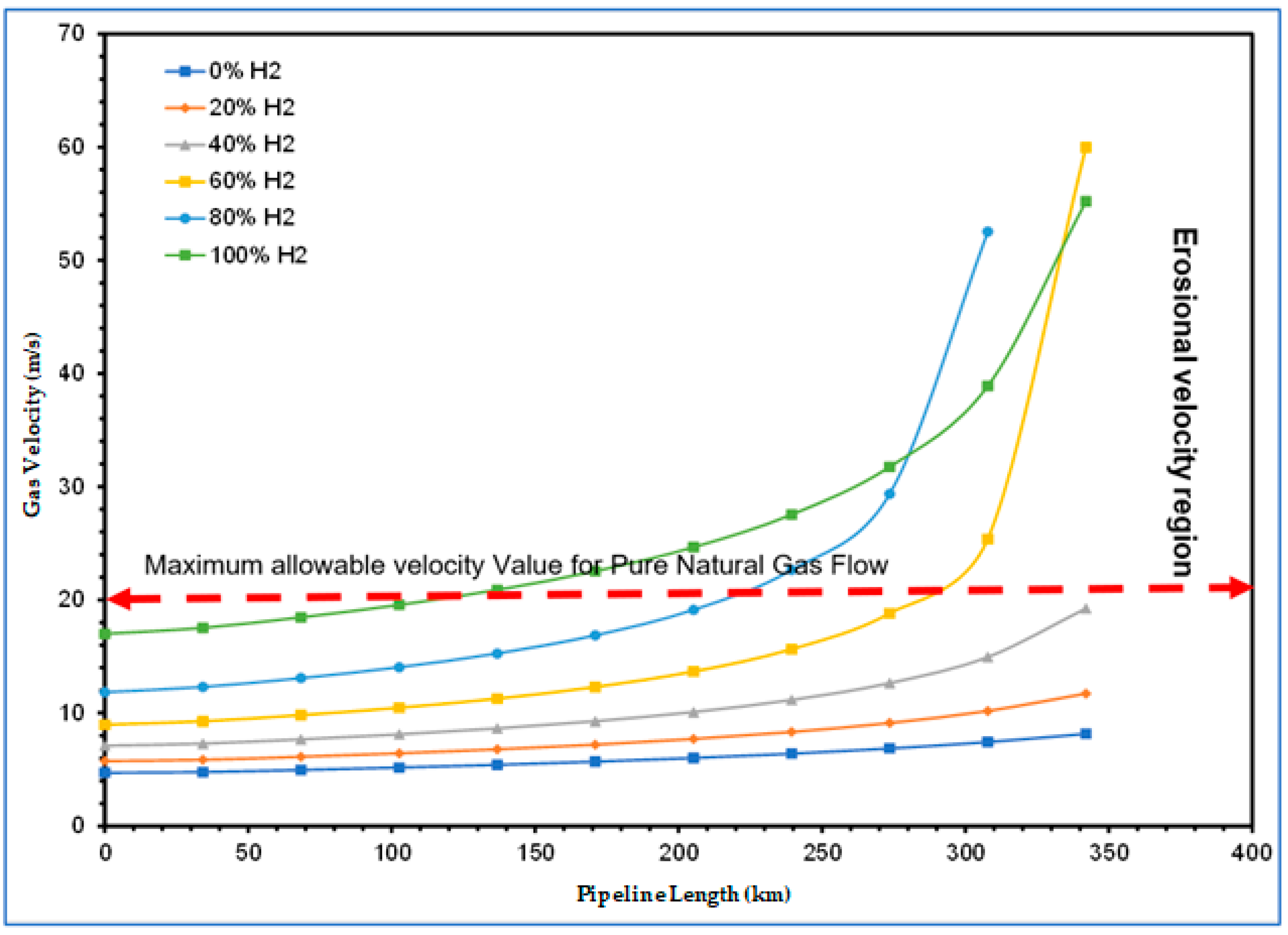
4.2.2. Hydrogen Blending Effect on Flow Velocity along High-pressure Gas Pipelines

As described in Section 3.2, velocity constraints were not imposed on the experiment for the free-flow stage. According to Figure 10, due to increasing pressure losses and consequent density reduction, the velocity recorded increased above the erosional velocity limit of 20 m/s for hydrogen contents greater or equal to 60% in the flow blend. This behaviour indicates that the pipeline could fail due to erosion. Two technical solutions to that are the use of compressor stations and pipeline looping. The result of adding a compressor station is presented in Section 4.3.

Once hydrogen is injected into the natural gas stream, even at 20% proportion, a gradual increase in velocity was observed due to the decrease in the density of the combined mixture. This trend continued for blends up to 40%, with the maximum velocity still within the allowable velocity limits for the entire 342 km pipe length. On the other hand, 60% hydrogen blends with natural gas will move the velocity–length graph into the region of erosional velocity limit for a pipe length as short as 290 km, as shown in Figure 10. This makes it necessary for compression or looping at that distance, which comes with additional cost to the energy transition scheme.

To better understand the nature of the hydrogen blends vis-à-vis the high-velocity profiles that pose safety concerns in the pipeline beyond the acceptable erosional limit, the nature of the density changes for each blend provides better insights. This is shown in Figure 11, where each arrow-headed dashed line shows the range of change in density for the curve with the same colour.

4.3. Velocity Profiles Behaviour with Compressor Stations in Existing Gas Pipeline Networks for Flow of Hydrogen and Hydrogen and Natural Gas Blends

Figure 12 shows that the pipeline velocity can be kept below the recommended 20 m/s natural gas pipeline erosional velocity limit for different proportions of hydrogen and natural gas blends (up to 80% of hydrogen concentration for the range of parameter utilized in this study) with the use of a single compressor station. It also shows that, for pure hydrogen flow, more than one compressor station would be required with the first compressor station positioned at 120 km length of the pipeline rather than 171 km, as the erosional velocity limit was exceeded before the latter.

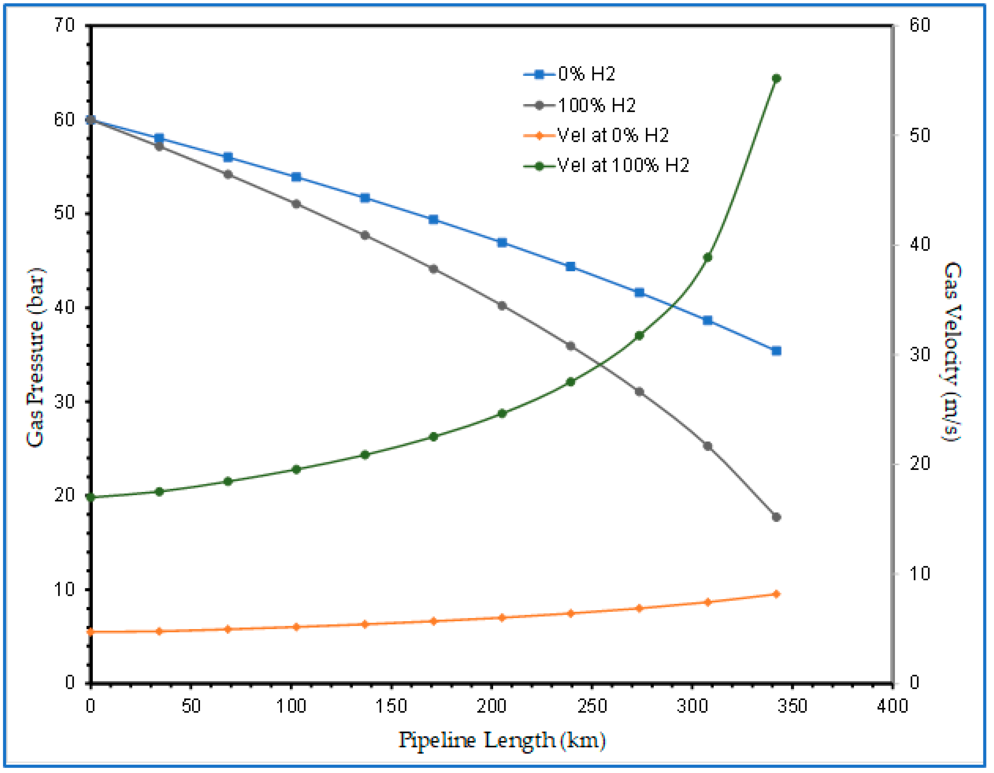
4.4. Downstream Pressure versus Velocity Trade-Off

Because of frictional losses along gas pipelines, introducing hydrogen with significantly lower molecular weight into a natural gas stream will increase the pressure loss and subsequently cause acceleration of the gas molecules under a constant energy delivery scenario. The free-flow scenario (Section 4.1) indicated an increase of up to three-fold volumetric flowrate requirement in the same pipeline, thereby creating higher frictional losses. The implication of this is that the hydrogen velocity increased up to ten-fold (from 6 m/s to 66 m/s), which is far beyond the maximum allowable velocity estimated as per API RP 14E. The trade-off of pressure versus velocities is indicated in Figure 13.

The trade-off behaviour between the pressure loss and velocity increase can be managed with the use of lower blends of hydrogen in natural gas.

5. Discussion

A key parameter in constant energy delivery when natural gas is to be substituted with hydrogen is the volume of hydrogen that will be required to deliver an equivalent amount of energy for a given volume of natural gas. For the parameters examined in this work, 570 MMSCFD of natural gas could be replaced by 1779 MMCSFD of hydrogen to deliver the same amount of energy—6440 MW. In other words, a given volume of natural gas would need to be tripled if the same amount of energy it generates is to be supplied by 100% hydrogen. This is attributable to the lower energy content of hydrogen (12 MJ/m³) compared to the energy content of natural gas (36 MJ/m³). Intermediate blends with 20, 40, 60, and 80% hydrogen proportions were also investigated.

In addition to concerns of volumetric requirements, safety is also a major deciding factor that deserves due cognisance in the transition from natural gas to hydrogen. The safety of a gas pipeline is hugely dependent on the flow behaviour of the gas stream, amongst other factors. For instance, the flow behaviour of gases in a constant diameter pipeline is expected to show increased pressure drop with higher pipeline capacity and increase in pipe length due to frictional drag along the walls of the pipeline [66,67]. As a result, density reduction, and consequent increase in gas velocity, is experienced in gas pipelines with increasing pipe length (or distance of travel of the gas) [28]; this is evident in Figure 10. Additionally worthy of note in Figure 10 is the hike in the rate of increase in the velocity profile for the curves signifying 60 and 80% hydrogen contents in the blend. This behaviour is attributable to the gross volumetric increase and the consequent density reduction, which occurs as the proportion of the lighter hydrogen phase exceeds that of natural gas in the blend. The extent to which this phenomenon can cause flow parameters (like the gas velocity) to deviate from the safe limits specified by international standards such as the API RP14E [56] has only been sparsely investigated, especially with regard to hydrogen transportation in natural gas pipelines.

Therefore, in this study, due attention was paid to the compressibility behaviour and the maximum velocity constraints for each simulation. The high-pressure losses and consequent high gas velocities noticed at the regions with ≥60% hydrogen in the results of the investigation of the velocity profile (Figure 10) revealed the potential of pipeline erosion at ≥60% hydrogen proportion in the blends; indicating that, within the range of parameters investigated in this study, hydrogen can be transported in natural gas pipelines by blending with natural gas by up to 40% without exceeding the erosional velocity limits of the pipeline. However, when the proportion of hydrogen reached 60%, the erosional velocity limit was reached at 290 km; so that, beyond this distance in the 342 km pipeline, the system would be subject to internal erosion.

To avoid this, an alternative to the use of a single, long pipeline would be to invest in additional compressor station(s) or pipeline looping for the transportation of such blends (the former option was used in this study to keep the velocity profile below the recommended erosional velocity limit of natural gas flow in pipelines for up to 80% hydrogen concentration in the natural gas blend). This is expedient because, in addition to the length of travel and pipe capacity, the introduction of hydrogen escalates the reduction in the density of the blends (see Figure 11). Therefore, attention should be paid to the maximum allowable flow velocity, with increasing hydrogen content, when designing for hydrogen transportation through blending with natural gas in existing gas pipeline infrastructure.

6. Conclusions

• This study explored the adoption of the existing natural gas pipelines for hydrogen delivery. A single pipeline flow was modelled to estimate the required volume of hydrogen needed to deliver the same amount of energy for a given volume of natural gas. Preliminary results from the study confirmed that a given volume of pure hydrogen gas would need to be tripled to deliver the same amount of energy as the same volume of natural gas, indicating the accuracy and validity of the model predictions.
• The second stage of the study also confirmed that an existing gas pipeline can accommodate hydrogen and natural gas blends with up to 40% hydrogen without the need for additional changes or investment in the pipeline infrastructure to mitigate internal erosion because the velocity profile was within the acceptable limits prescribed by API RP 14E. However, as the proportion of hydrogen in the blends was increased up to and beyond 60%, excessive pressure losses became eminent. This was characterised by the rising velocity, which eventually exceeded the erosional velocity limits before the gas reached the discharge point. This is a cause for concern because the pipeline could fail earlier than it is designed to last. To remedy this, technical solutions of using compressor stations or pipeline looping are recommended.
• A third objective of the study that investigated the effect of hydrogen blending on the behaviour of the compressibility factor also revealed that the compressibility factor could possess a wide range of values as the proportions of hydrogen and natural gas in the blends change. Consequently, disparate flow behaviours and resultant varying flow challenges would be faced when transporting hydrogen blends within existing pipelines.
• In a nutshell, this study has shown that increasing the capacity of a hydrogen pipeline by up to three-folds of a given capacity of an existing natural gas pipeline will result in the delivery of the same amount of energy but present peculiar flow behaviours and challenges that are different from those observed in conventional natural gas pipelines. This work, therefore, provides insights into the volumetric and safety considerations of designing hydrogen transportation through pipelines by blending with natural gas as the global community considers the replacement of natural gas with hydrogen in the energy transition and decarbonisation campaigns.

References

1. Staffel, I.; Scamman, D.; Abdad, A.V.; Balcombe, P.; Dodds, P.E.; Ekins, P.; Shahd, N.; Ward, R.K. The role of hydrogen and fuel cells in the global energy system. Energy Environ. Sci. 2019, 12, 463. [Google Scholar] [CrossRef] [Green Version]
2. Bossel, U. Does a Hydrogen Economy Make Sense? Proc. IEEE 2006, 94, 1826–1836. [Google Scholar] [CrossRef]
3. Jones, D.R.; Al-Masry, W.A.; Dunnill, C.W. Hydrogen-enriched natural gas as a domestic fuel: An analysis based on flash-back and blow-off limits for domestic natural gas appliances within the UK. Sustain. Energy Fuels 2018, 2, 710–723. [Google Scholar] [CrossRef] [Green Version]
4. Witkowski, A.; Rusin, A.; Majkut, M.; Stolecka, K. Comprehensive analysis of hydrogen compression and pipeline transportation from thermodynamics and safety aspects. Energy 2017, 141, 2508–2518. [Google Scholar] [CrossRef]
5. Bainier, F.; Kurz, R.; Bass, P. Managing the pressure to increase the H2 capacity through a natural gas transmission network. Proc. ASME Turbo Expo 2020, 9, 1–9. [Google Scholar]
6. André, J.; Auray, S.; De Wolf, D.; Memmah, M.M.; Simonnet, A. Time development of new hydrogen transmission pipeline networks for France. Int. J. Hydrogen Energy 2014, 39, 10323–10337. [Google Scholar] [CrossRef] [Green Version]
7. Guandalini, G.; Colbertaldo, P.; Campanari, S. Dynamic modeling of natural gas quality within transport pipelines in presence of hydrogen injections. Appl. Energy 2017, 185, 1712–1723. [Google Scholar] [CrossRef]
8. Xu, J.; Zhang, X.; Liu, J.; Fan, L. Experimental study of a single-cylinder engine fueled with natural gas-hydrogen mixtures. Int. J. Hydrogen Energy 2010, 35, 2909–2914. [Google Scholar] [CrossRef]
9. Di Lullo, G.; Oni, A.O.; Kumar, A. Blending blue hydrogen with natural gas for direct consumption: Examining the effect of hydrogen concentration on transportation and well-to-combustion greenhouse gas emissions. Int. J. Hydrogen Energy 2021, 46, 19202–19216. [Google Scholar] [CrossRef]
10. Çeper, B.A. Use of Hydrogen-Methane Blends in Internal Combustion Engines. In Hydrogen Energy—Challenges and Perspectives; IntechOpen: London, UK, 2012; pp. 175–200. [Google Scholar]
11. Economides, M.J.; Hill, A.D.; Ehlig-Economides, C. Petroleum Production Systems; Prentice Hall Petroleum Engineering Series; Sun, B., Trentacoste, C., Intindola, K., Eds.; Pearson: London, UK, 1994; ISBN 0-13-658683-X. [Google Scholar]
12. Ahmed, T. Reservoir Engineering Handbook, 2nd ed.; Gulf Professional Publishing: Houston, TX, USA, 2001; ISBN 0884157709. [Google Scholar]
13. Folga, S.M. Natural Gas Pipeline Technology Overview; Argonne National Laboratory: Argonne, IL, USA, 2007. [Google Scholar]
14. Gerboni, R. Introduction to hydrogen transportation. In Compendium of Hydrogen Energy; Elsevier: Amsterdam, The Netherlands, 2016; pp. 283–298. [Google Scholar]
15. Seymour, E.H.; Murray, L.; Fernandes, R. Key Challenges to the introduction of hydrogen-European stakeholder views. Int. J. Hydrogen Energy 2008, 33, 3015–3020. [Google Scholar] [CrossRef]
16. Gillette, J.; Kolpa, R. Overview of Interstate Hydrogen Pipeline Systems; Argonne National Laboratory: Argonne, IL, USA, 2007; p. 52. [Google Scholar]
17. Hydrogen Pipeline Length by Country|Statista. 2016. Available online: https://www.statista.com/statistics/1147797/hydrogen-pipeline-length-by-country/ (accessed on 17 August 2021).
18. Department of Energy US. Enabling A Low-Carbon Economy; Department of Energy US: Washington, DC, USA, 2020; p. 24. Available online: https://www.energy.gov/sites/prod/files/2020/07/f76/USDOE_FE_Hydrogen_Strategy_July2020.pdf (accessed on 15 September 2021).
19. IRENA Hydrogen: A Renewable Energy Perspective; International Renewable Energy Agency: Abu Dhabi, United Arab Emirates, 2019; ISBN 9789292601515.
20. Field, R.A.; Derwent, R.G. Global warming consequences of replacing natural gas with hydrogen in the domestic energy sectors of future low-carbon economies in the United Kingdom and the United States of America. Int. J. Hydrogen Energy 2021, 46, 30190–30203. [Google Scholar] [CrossRef]
21. Petak, K.; Vidas, H.; Manik, J.; Palagummi, S.; Ciatto, A.; Griffith, A. Infrastructure Investment an Engine for Economic Growth; American Petroleum Institute (API): Washington, DC, USA, 2017. [Google Scholar]
22. Parker, N. Using Natural Gas Transmission Pipeline Costs to Estimate Hydrogen Pipeline Costs; Institute of Transportation Studies, University of California: Davis, CA, USA, 2015; p. 27. [Google Scholar]
23. Witkowski, A.; Rusin, A.; Majkut, M.; Stolecka, K. Analysis of compression and transport of the methane/hydrogen mixture in existing natural gas pipelines. Int. J. Press. Vessel. Pip. 2018, 166, 24–34. [Google Scholar] [CrossRef]
24. Oney, F.; Veziro~lut, T.N.; Dulger, Z. Evaluation of pipeline transportation of hydrogen and natural gas mixtures. Int. J. Hydrogen Energy 1994, 19, 813–822. [Google Scholar] [CrossRef]
25. Quintino, F.M.; Nascimento, N.; Fernandes, E.C. Aspects of Hydrogen and Biomethane Introduction in Natural Gas Infrastructure and Equipment. Hydrogen 2021, 2, 301–318. [Google Scholar] [CrossRef]
26. Chen, T.P. Hydrogen Delivery Infrastructure Options Analysis; DOE Award Number: DE-FG36-05GO15032; Nexant, Inc.: San Francisco, CA, USA, 2008. [Google Scholar]
27. Melaina, M.W.; Antonia, O.; Penev, M. Blending Hydrogen into Natural Gas Pipeline Networks: A Review of Key Issues; Technical Report NREL/TP-5600-51995; National Renewable Energy Laboratory: Golden, CO, USA, 2013; Volume 303, pp. 275–3000. Available online: http://www.osti.gov/servlets/purl/1068610/ (accessed on 6 September 2021).
28. Ahmed, T. Reservoir Engineering Handbook, 4th ed.; Gulf Professional Publishing: Oxford, UK, 2010; Volume 27. [Google Scholar]
29. Nasir, G.G. Gas Flow and Network Analysis. In Gas Flow in Circular Pipes; Department of Gas Engineering and Management, University of Salford, Manchester: Manchester, UK, 2002; Volume 1, pp. 1–6. [Google Scholar]
30. Li, J.; Su, Y.; Yu, B.; Wang, P.; Sun, D. Influences of Hydrogen Blending on the Joule-Thomson Coefficient of Natural Gas. ACS Omega 2021, 6, 16722–16735. [Google Scholar] [CrossRef]
31. Simpson, D.A. Practical Onshore Gas Field Engineering; Gulf Professional Publishing: Oxford, UK, 2017; ISBN 9780128130223. [Google Scholar]
32. Guo, B.; Ghalambor, A. Properties of Natural Gas. In Natural Gas Engineering Handbook; Elsevier: Amsterdam, The Netherlands, 2005; Volume 97, pp. 13–33. [Google Scholar]
33. Mouser, G.F.; Govier, J.P. Compressibility Effects on Transient Gas Pipe Flow. Soc. Pet. Eng. J. 1972, 12, 315–320. [Google Scholar] [CrossRef]
34. Farzaneh-Gord, M.; Rahbari, H.R.; Mohseni-Gharesafa, B.; Toikka, A.; Zvereva, I. Accurate determination of natural gas compressibility factor by measuring temperature, pressure and Joule-Thomson coefficient: Artificial neural network approach. J. Pet. Sci. Eng. 2021, 202, 108427. [Google Scholar] [CrossRef]
35. Khosravi, A.; Machado, L.; Nunes, R.O. Estimation of density and compressibility factor of natural gas using artificial intelligence approach. J. Pet. Sci. Eng. 2018, 168, 201–216. [Google Scholar] [CrossRef]
36. Liu, H.; Wu, Y.; Guo, P.; Liu, Z.; Wang, Z.; Chen, S.; Wang, B.; Huang, Z. Compressibility factor measurement and simulation of five high-temperature ultra-high-pressure dry and wet gases. Fluid Phase Equilib. 2019, 500, 112256. [Google Scholar] [CrossRef]
37. USDrive. Hydrogen Delivery Technical Team Roadmap. 2013. Available online: www.uscar.org (accessed on 18 August 2021).
38. Nykyforchyn, H.; Tsyrulnyk, O.; Zvirko, O. Laboratory method for simulating hydrogen assisted degradation of gas pipeline steels. Procedia Struct. Integr. 2019, 17, 568–575. [Google Scholar] [CrossRef]
39. Dwivedi, S.K.; Vishwakarma, M. Hydrogen embrittlement in different materials: A review. Int. J. Hydrogen Energy 2018, 43, 21603–21616. [Google Scholar] [CrossRef]
40. Wasim, M.; Djukic, M.B.; Ngo, T.D. Influence of hydrogen-enhanced plasticity and decohesion mechanisms of hydrogen embrittlement on the fracture resistance of steel. Eng. Fail. Anal. 2021, 123, 105312. [Google Scholar] [CrossRef]
41. Ogden, J.M. Prospects for building a hydrogen energy infrastructure. Annu. Rev. Energy Environ. 1999, 24, 227–279. [Google Scholar] [CrossRef]
42. Abd, A.A.; Naji, S.Z.; Thian, T.C.; Othman, M.R. Evaluation of hydrogen concentration effect on the natural gas properties and flow performance. Int. J. Hydrogen Energy 2021, 46, 974–983. [Google Scholar] [CrossRef]
43. American Petroleum Institute. Recommended Practice for Design and Installation of Offshore Production Platform Piping Systems, 5th ed.; American Petroleum Institute: Washington, DC, USA, 2012; pp. 23–26. [Google Scholar]
44. Nasr, G.G.; Connor, N.E. Natural Gas Engineering and Safety Challenges: Downstream Process, Analysis, Utilization and Safety; Springer: Berlin/Heidelberg, Germany, 2014; ISBN 9783319089485. [Google Scholar]
45. Andrade-Mahecha, J.F.; Massy-Sanchez, G.I. Simulation of the operation of a natural gas transport system based on a criterion of minimum operating cost. DYNA 2019, 86, 308–316. [Google Scholar] [CrossRef] [Green Version]
46. Osiadacz, A.J.; Isoli, N. Multi-Objective Optimization of Gas Pipeline Networks. Energies 2020, 13, 5141. [Google Scholar] [CrossRef]
47. Munoz, J.; Jimenez-Redondo, N.; Perez-Ruiz, J.; Barquin, J. Natural gas network modeling for power systems reliability studies. In Proceedings of the 2003 IEEE Bologna Power Tech Conference, Bologna, Italy, 23–26 June 2003; Volume 4, pp. 20–27. [Google Scholar]
48. Tabkhi, F. Optimization of Gas Transmission Networks; National Polytechnique Institute of Toulouse: Toulouse, France, 2007. [Google Scholar]
49. Dorin, B.C.; Leonida, D.T. On Modelling and Simulating Natural Gas Transmission Systems (Part 1). J. Control Eng. Appl. Inform. 2008, 10, 27–36. Available online: https://www.researchgate.net/publication/228661898%0AOn (accessed on 8 September 2021).
50. Woldeyohannes, A.D.; Majid, M.A.A. Simulation model for natural gas transmission pipeline network system. Simul. Model. Pract. Theory 2011, 19, 196–212. [Google Scholar] [CrossRef]
51. Stoecker, W.F. Design of Thermal System; McGraw-Hill Book Company: New York, NY, USA, 1989; ISBN 0070616205. [Google Scholar]
52. Abbaspour, M.; Chapman, K.S.; Glasgow, L.A. Transient modeling of non-isothermal, dispersed two-phase flow in natural gas pipelines. Appl. Math. Model. 2010, 34, 495–507. [Google Scholar] [CrossRef]
53. Kessal, M. Simplified numerical simulation of transients in gas networks. Chem. Eng. Res. Des. 2000, 78, 925–931. [Google Scholar] [CrossRef] [Green Version]
54. Badr, E.; Almotairi, S.; Ghamry, A. El A comparative study among new hybrid root finding algorithms and traditional methods. Mathematics 2021, 9, 1306. [Google Scholar] [CrossRef]
55. Ehiwario, J.C.; Aghamie, S.O. Comparative Study of Bisection, Newton-Raphson and Secant Methods of Root-Finding Problems. IOSR J. Eng. 2014, 4, 1–7. [Google Scholar]
56. Recommended Practice for Design and Installation of Offshore Production Platform Piping Systems; API-RP-14E; American Petroleum Institute Production: Washington, DC, USA, 1991; p. 11.
57. Herrán-González, A.; De La Cruz, J.M.; De Andrés-Toro, B.; Risco-Martín, J.L. Modeling and simulation of a gas distribution pipeline network. Appl. Math. Model. 2009, 33, 1584–1600. [Google Scholar] [CrossRef]
58. Alliander, W. Gas Distribution Network Modelling and Optimization—New Methods for Smarter Observation and Operation of Large Scale Gas Networks; Delft University of Technology (TUDelft): Delft, The Netherlands, 2016. [Google Scholar]
59. Ashour, I.; Al-Rawahi, N.; Fatemi, A.; Vakili-Nezh, G. Applications of Equations of State in the Oil and Gas Industry. In Thermodynamics—Kinetics of Dynamic Systems; IntechOpen: London, UK, 2011. [Google Scholar] [CrossRef] [Green Version]
60. Esmaeilzadeh, F.; Roshanfekr, M. A new cubic equation of state for reservoir fluids. Fluid Phase Equilib. 2006, 239, 83–90. [Google Scholar] [CrossRef]
61. Bonyadi, M.; Rahimpour, M.R.; Esmaeilzadeh, F. A new fast technique for calculation of gas condensate well productivity by using pseudopressure method. J. Nat. Gas Sci. Eng. 2012, 4, 35–43. [Google Scholar] [CrossRef]
62. Beggs, H.D.; Brill, J.R. A Study of Two-Phase Flow in Inclined Pipes. J. Pet. Technol. 1973, 25, 607–617. [Google Scholar] [CrossRef]
63. Ahmed, M.M.; Ayoub, M.A. A Comprehensive Study on the Current Pressure Drop Calculation in Multiphase Vertical Wells; Current Trends and Future Prospective. J. Appl. Sci. 2014, 14, 3162–3171. [Google Scholar] [CrossRef] [Green Version]
64. Colebrook, C.F.; White, C.M. The Reduction of Carrying Capacity of Pipes with Age. J. Inst. Civ. Eng. 1937, 7, 99–118. [Google Scholar] [CrossRef]
65. Abohamzeh, E.; Salehi, F.; Sheikholeslami, M.; Abbassi, R.; Khan, F. Review of hydrogen safety during storage, transmission, and applications processes. J. Loss Prev. Process Ind. 2021, 72, 104569. [Google Scholar] [CrossRef]
66. Sani, F.M.; Nesic, S. Review of the API RP 14E Erosional Velocity Equation: Origin, Applications, Mis-uses and Limitations. In Proceedings of the NACE International Corrosion Conference and Expo 2019, Nashville, TN, USA, 24–28 March 2019; Volume 148, pp. 148–162. [Google Scholar]
67. Yang, Z.; Fahmi, A.; Drescher, M.; Teberikler, L.; Merat, C.; Langsholt, M.; Liu, L. Improved understanding of flow assurance for CO2 transport and injection. In Proceedings of the 15th Greenhouse Gas Control Technologies Conference, Online, 15–18 March 2021; pp. 1–2. [Google Scholar]
Figure 1. Energy contents of natural gas (NG) and hydrogen (H2) blends.
Gases 01 00013 g001
Figure 2. Gas pressure versus length ( Q ( a ) < Q ( b ) < Q ( c ) < Q D ).
Gases 01 00013 g002
Figure 3. Typical velocity profile behaviour in gas pipelines.
Gases 01 00013 g003
Figure 4. Simulation flow chart for pipeline transportation of hydrogen and natural gas blends.
Gases 01 00013 g004
Figure 5. Free-flow pipeline model.
Gases 01 00013 g005
Figure 6. Compressor station option model for 80% hydrogen and 20% natural gas blend.
Gases 01 00013 g006
Figure 7. Compressor station option model for 100% hydrogen.
Gases 01 00013 g007
Figure 8. Volumetric requirements of natural gas and hydrogen for a constant supply of 6440 MW energy value (the intercept of the curve on the vertical axis indicates 100% natural gas).
Gases 01 00013 g008
Figure 9. Compressibility behaviour of hydrogen blends.
Gases 01 00013 g009
Figure 10. Velocity profile for gas pipeline flow of hydrogen blends (60 bar, 303.15 K).
Gases 01 00013 g010
Figure 11. Gas density trends along the pipeline (arrow-headed dashed lines show the range of change in density for the curves with the same colour).
Gases 01 00013 g011
Figure 12. Velocity profiles of hydrogen and hydrogen blends in gas pipelines with a single compressor station (60 bar, 303.15 K).
Gases 01 00013 g012
Figure 13. Trade-off of pressure versus velocities in the hydrogen blend pipeline
Gases 01 00013 g013