
Impact of Managed-Lane Pricing Strategies on Vehicle-Sourced NOx and HC Emissions


Abstract
:
1. Motivation and Related Works
2. Methodology
2.1. Data Collection
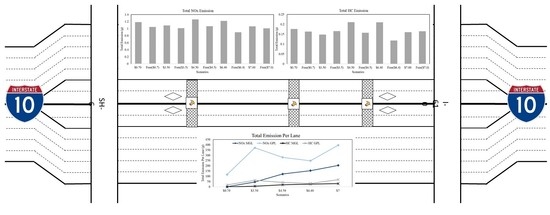
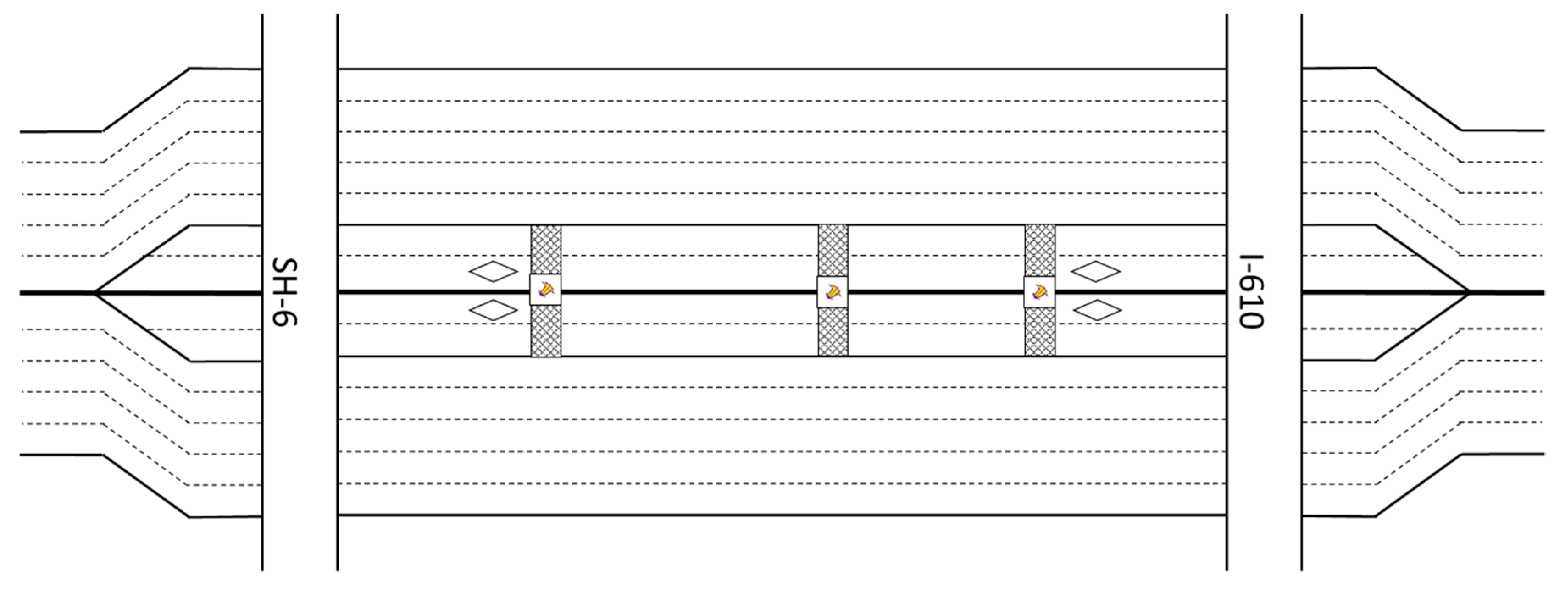
2.1.1. Test Route Information
- 3.5 USD for weekdays 9:00–10:00 a.m. Eastbound;
- 4.5 USD for weekdays 6:00–7:00 a.m. Eastbound and 3:00–4:00 p.m., 6:00–7:00 p.m. Westbound;
- 6.4 USD for weekdays 8:00–9:00 a.m. Eastbound;
- 7 USD for weekdays 7:00–8:00 a.m. Eastbound and 4:00–6:00 p.m. Westbound; and
- 0.7 USD for all other times.
2.1.2. Test Plan
2.2. Vehicle Emission Calculation
3. Case Study Data Analysis
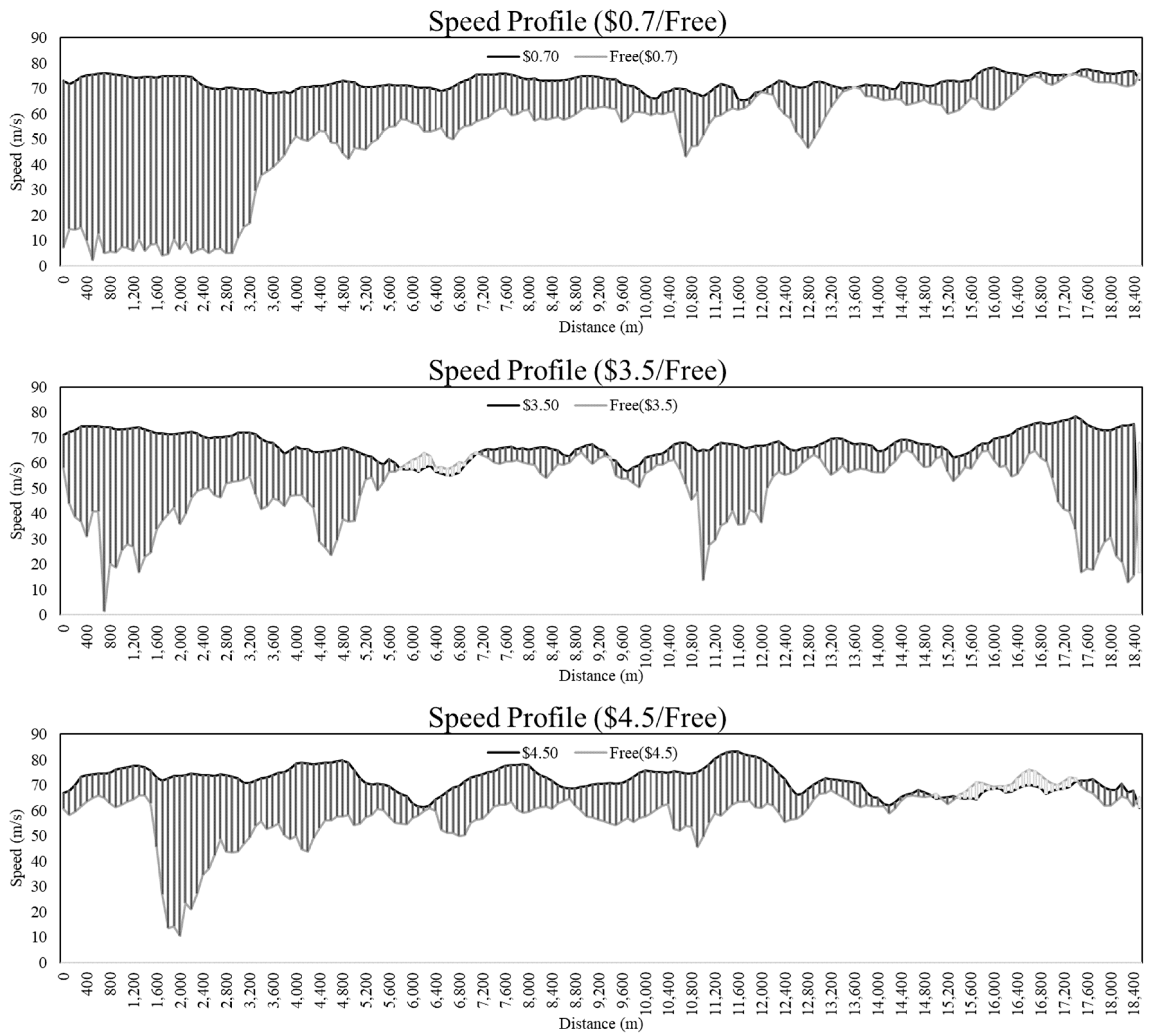
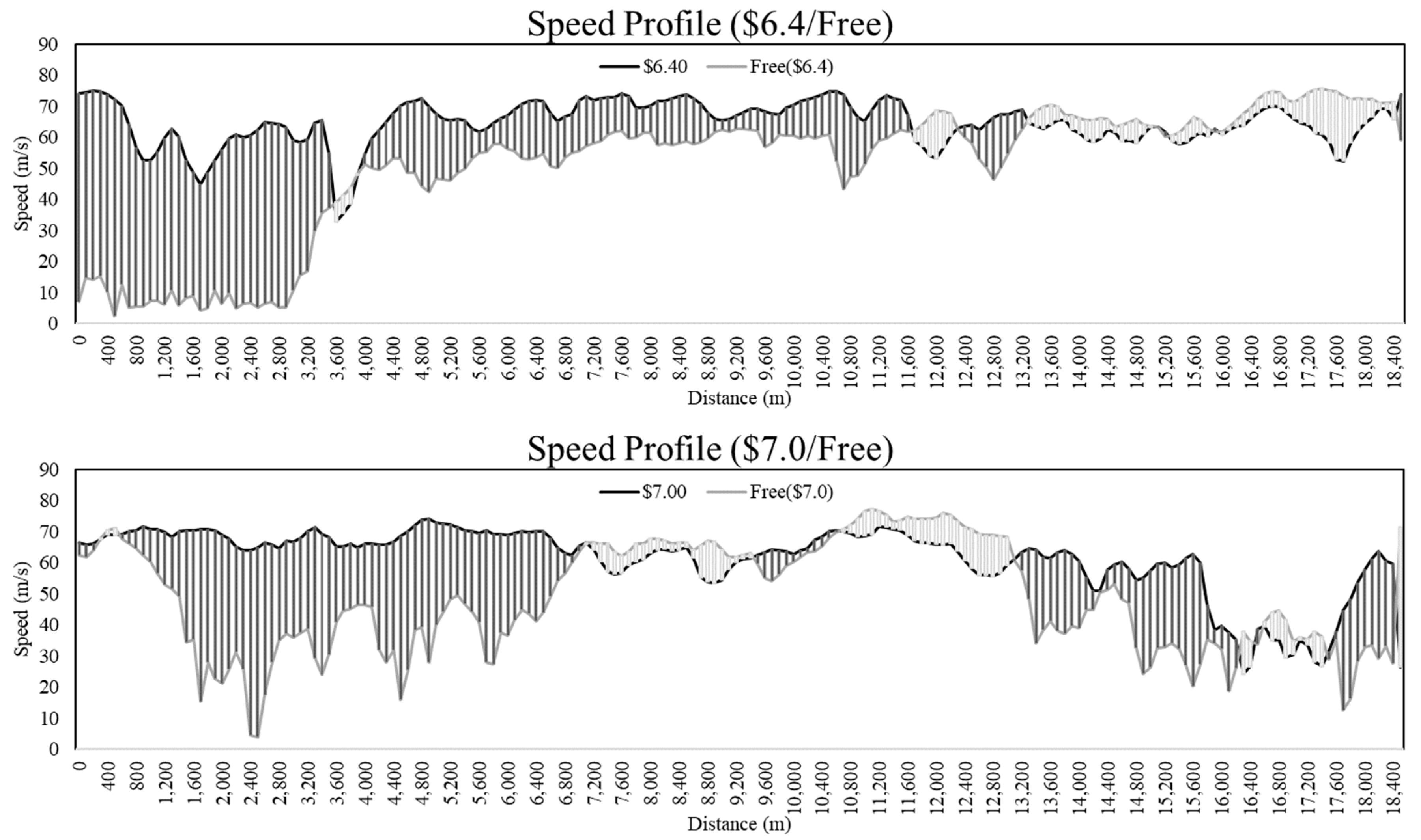
3.1. Speed Profile Analysis
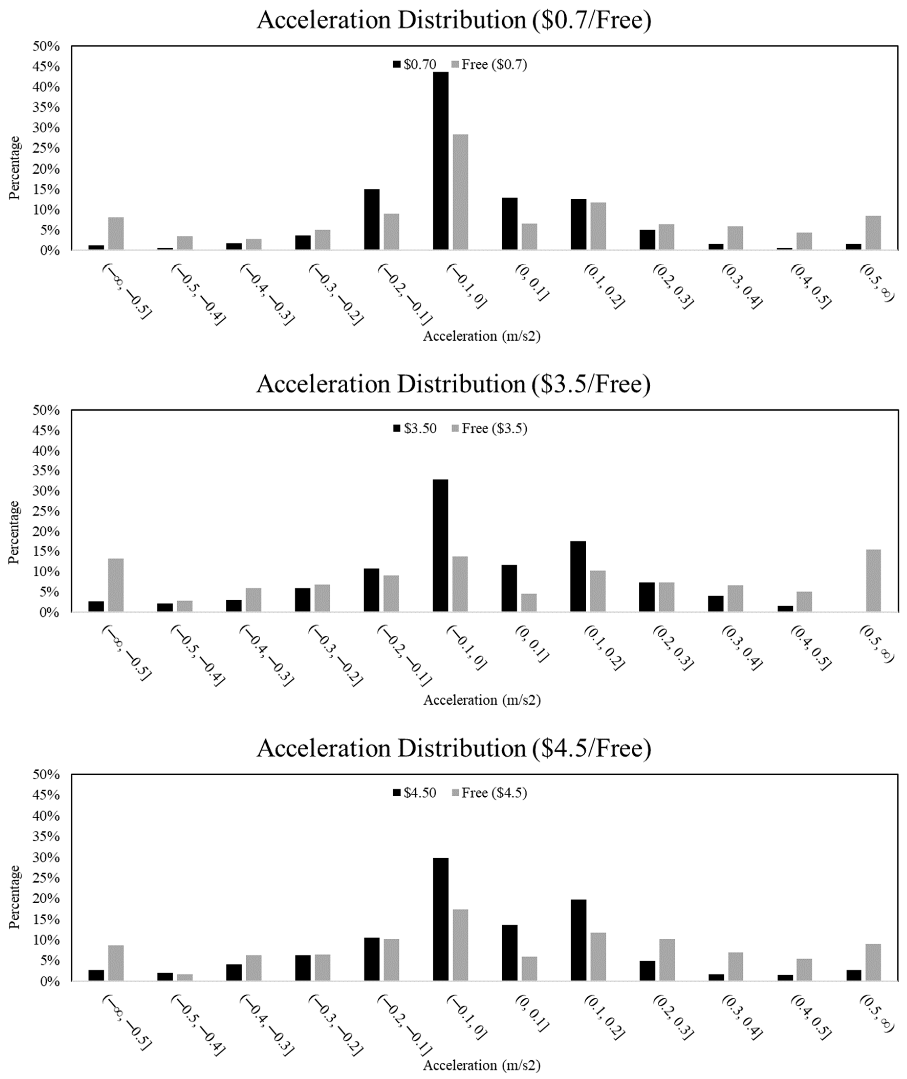
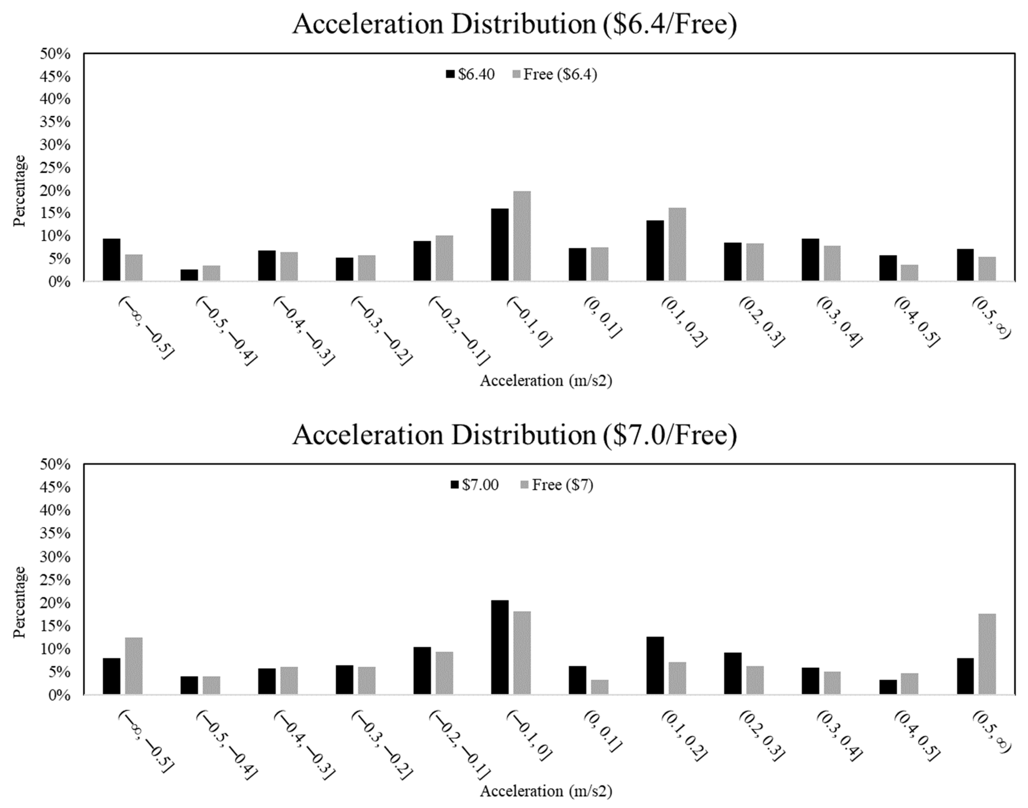
3.2. Acceleration Profile Analysis
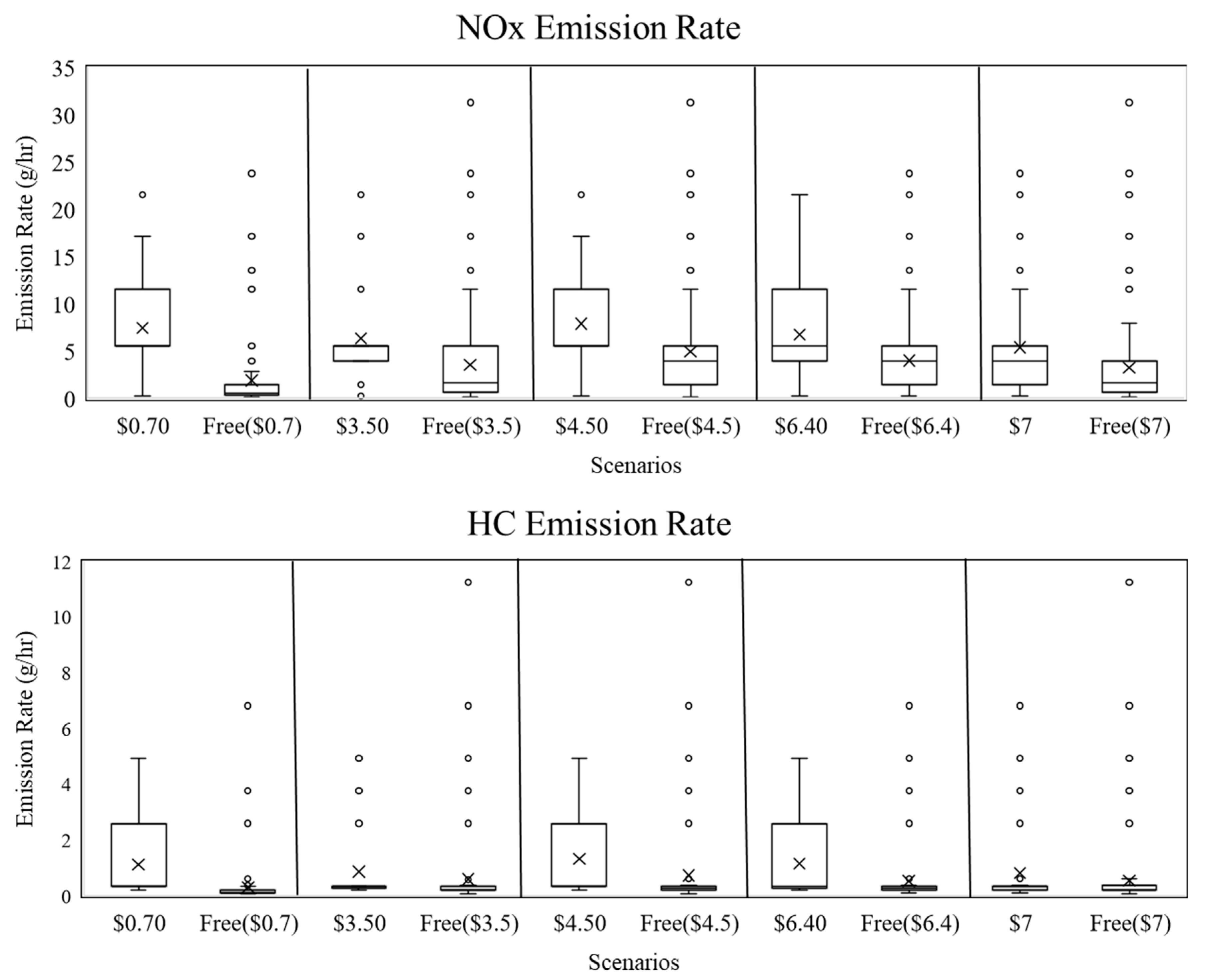
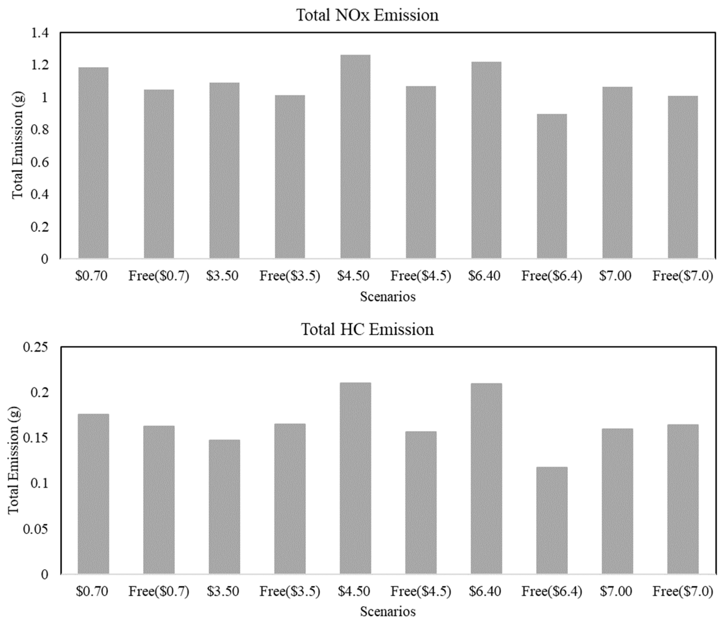
3.3. Emission Analysis
4. Conclusions
Author Contributions
Funding
Acknowledgments
Conflicts of Interest
References
- Schlink, U.; Herbarth, O.; Richter, M.; Dorling, S.; Nunnari, G.; Cawley, G.; Pelikan, E. Statistical models to assess the health effects and to forecast ground-level ozone. Environ. Model. Softw. 2006, 21, 547–558. [Google Scholar] [CrossRef]
- Shao, M.; Zhang, Y.; Zeng, L.; Tang, X.; Zhang, J.; Zhong, L.; Wang, B. Ground-level ozone in the Pearl River Delta and the roles of VOC and NOx in its production. J. Environ. Manag. 2009, 90, 512–518. [Google Scholar] [CrossRef]
- Guttorp, P.; Meiring, W.; Sampson, P.D. A space-time analysis of ground-level ozone data. Environmetrics 1994, 5, 241–254. [Google Scholar] [CrossRef]
- Du, J.; Qiao, F.; Yu, L. Temporal characteristics and forecasting of PM2.5 concentration based on historical data in Houston, USA. Resour. Conserv. Recycl. 2019, 147, 145–156. [Google Scholar] [CrossRef]
- Lippmann, M. Health effects of ozone. A Critical Review. JAPCA 1989, 39, 672–695. [Google Scholar] [CrossRef] [Green Version]
- Bell, M.L.; McDermott, A.; Zeger, S.L.; Samet, J.M.; Dominici, F. Ozone and short-term mortality in 95 US urban communities. 1987–2000. JAMA 2004, 292, 2372–2378. [Google Scholar] [CrossRef] [PubMed] [Green Version]
- Lake, G.J. Ozone Cracking and Protection of Rubber. Rubber Chem. Technol. 1970, 43, 1230–1254. [Google Scholar] [CrossRef]
- Shindell, E.T.; Rind, D.; Lonergan, P. Increased polar stratospheric ozone losses and delayed eventual recovery owing to increasing greenhouse-gas concentrations. Nat. Cell Biol. 1998, 392, 589–592. [Google Scholar] [CrossRef]
- Cardelino, C.; Chameides, W. An Observation-Based Model for Analyzing Ozone Precursor Relationships in the Urban Atmosphere. J. Air Waste Manag. Assoc. 1995, 45, 161–180. [Google Scholar] [CrossRef] [PubMed]
- Abdul-Wahab, S.A.; Bakheit, C.S.; Al-Alawi, S.M. Principal component and multiple regression analysis in modelling of ground-level ozone and factors affecting its concentrations. Environ. Model. Softw. 2005, 20, 1263–1271. [Google Scholar] [CrossRef]
- FHWA. Annual Vehicle Distance Traveled in Miles and Related Data—2016 by Highway Category and Vehicle Type; F.H. Administration: Washington, DC, USA, 2017.
- Carlson, R.C.; Papamichail, I.; Papageorgiou, M.; Messmer, A. Optimal motorway traffic flow control involving variable speed limits and ramp metering. Transp. Sci. 2010, 44, 238–253. [Google Scholar] [CrossRef]
- Guo, X.; Peng, Y.; Ashraf, S.; Burris, M.W. Performance Analyses of Information-Based Managed Lane Choice Decisions in a Connected Vehicle Environment. Transp. Res. Rec. J. Transp. Res. Board 2020, 2674, 120–133. [Google Scholar] [CrossRef]
- Zhong, Z.; Lee, J. The effectiveness of managed lane strategies for the near-term deployment of cooperative adaptive cruise control. Transp. Res. Part A Policy Pract. 2019, 129, 257–270. [Google Scholar] [CrossRef] [Green Version]
- Kim, J.; Park, S.; Na, S.; Lee, S. Sustainable Highway Operations: High Occupancy Lane and Movable Lane. Int. J. Transp. 2015, 3, 1–10. [Google Scholar] [CrossRef]
- Yin, Y.; Lou, Y. Dynamic Tolling Strategies for Managed Lanes. J. Transp. Eng. 2009, 135, 45–52. [Google Scholar] [CrossRef]
- Ungemah, D.; Goodin, G.; Dusza, C.; Burris, M. Examining incentives and preferential treatment of carpools on managed lane facilities. J. Public Transp. 2007, 10, 8. [Google Scholar] [CrossRef] [Green Version]
- Bai, X.; Zhou, Z.; Chin, K.-S.; Huang, B. Evaluating lane reservation problems by carbon emission approach. Transp. Res. Part D Transp. Environ. 2017, 53, 178–192. [Google Scholar] [CrossRef]
- Bigazzi, A.Y.; Rouleau, M. Can traffic management strategies improve urban air quality? A review of the evidence. J. Transp. Health 2017, 7, 111–124. [Google Scholar] [CrossRef]
- Du, J.; Li, Q.; Yu, F.Q.L. Vehicle Emission Estimation On Mainline Freeway Under Isolated And Integrated Ramp Metering Strategies. Environ. Eng. Manag. J. 2018, 17, 1237–1248. [Google Scholar] [CrossRef]
- EPA. Air Emissions Sources; EPA: Washington, DC, USA, 2019.
- Shinar, D. Traffic Safety and Human Behavior; Emerald Publishing Limited: Bingley, UK, 2017. [Google Scholar]
- Council, N.R. Ozone-Forming Potential of Reformulated Gasoline; National Academies Press: Washington, DC, USA, 1999. [Google Scholar]
- Curran, M.A. Life Cycle Assessment Handbook: A Guide for Environmentally Sustainable Products; John Wiley & Sons: Hoboken, NJ, USA, 2012. [Google Scholar]
- Manes, F.; Incerti, G.; Salvatori, E.; Vitale, M.; Ricotta, C.; Costanza, R. Urban ecosystem services: Tree diversity and stability of tropospheric ozone removal. Ecol. Appl. 2012, 22, 349–360. [Google Scholar] [CrossRef] [PubMed]
- Taylor, C.E.; Benedick, R.E. Ozone Diplomacy; Harvard University Press: Cambridge, MA, USA, 1998. [Google Scholar]
- Jiang, W.; Boltze, M.; Groer, S.; Scheuvens, D. Impacts of low emission zones in Germany on air pollution levels. Transp. Res. Procedia 2017, 25, 3370–3382. [Google Scholar] [CrossRef]
- Barnes, J.H.; Chatterton, T.J.; Longhurst, J.W. Emissions vs exposure: Increasing injustice from road traffic-related air pollution in the United Kingdom. Transp. Res. Part D Transp. Environ. 2019, 73, 56–66. [Google Scholar] [CrossRef]
- Collier, T.; Goodin, G.D. Developing a Managed Lanes Position Paper for a Policy-Maker Audience; The National Academies of Sciences, Engineering, and Medicine: Washington, DC, USA, 2002. [Google Scholar]
- Avelar, R.; Fitzpatrick, K.; Dixon, K.; Lindheimer, T. The Influence of General Purpose Lane Traffic on Managed Lane Speeds: An Operational Study in Houston, Texas. Transp. Res. Procedia 2016, 15, 548–560. [Google Scholar] [CrossRef] [Green Version]
- Pandey, V.; Boyles, S.D. Dynamic pricing for managed lanes with multiple entrances and exits. Transp. Res. Part C Emerg. Technol. 2018, 96, 304–320. [Google Scholar] [CrossRef]
- Perez, B.G.; Fuhs, C.; Gants, C.; Giordano, R.; Ungemah, D.H.; Berman, W. Priced Managed Lane Guide; Federal Highway Administration: Washington, DC, USA, 2012. [Google Scholar]
- Perez, B.G.; Sciara, G.-C.; Parsons, B. A Guide for HOT Lane Development; Federal Highway Administration: Washington, DC, USA, 2002. [Google Scholar]
- Sinprasertkool, A. A New Paradigm in User Equilibrium—Application in Managed Lane Pricing. Ph.D. Thesis, University of Texas Arlington, Arlington, TX, USA, 2010. [Google Scholar]
- Stuart, A.; Lin, P.S.; Lee, C.; Yu, H.; Chen, H. Assessing Air Quality Impacts of Managed Lanes. In Proceedings of the 17th ITS World Congress ITS Japan ITS America ERTICO, Busan, Korea, 25–29 October 2010. [Google Scholar]
- Bigazzi, A.Y.; Figliozzi, M.A. Study of Emissions Benefits of Commercial Vehicle Lane Management Strategies. Transp. Res. Rec. J. Transp. Res. Board 2013, 2341, 43–52. [Google Scholar] [CrossRef] [Green Version]
- Stuart, A. Assessing Air Quality Impacts of Managed Lanes; University of South Florida Libraries: Tampa, FL, USA, 2010. [Google Scholar]
- Xu, Y.; Liu, H.; Rodgers, M.O.; Guin, A.; Hunter, M.; Sheikh, A.; Guensler, R. Understanding the emission impacts of high-occupancy vehicle (HOV) to high-occupancy toll (HOT) lane conversions: Experience from Atlanta, Georgia. J. Air Waste Manag. Assoc. 2017, 67, 910–922. [Google Scholar] [CrossRef] [PubMed]
- Haman, C.; Couzo, E.; Flynn, J.H.; Vizuete, W.; Heffron, B.; Lefer, B.L. Relationship between boundary layer heights and growth rates with ground-level ozone in Houston, Texas. J. Geophys. Res. Atmos. 2014, 119, 6230–6245. [Google Scholar] [CrossRef]
- USDOT. High-Occupancy Vehicle Lanes; USDOT: Washington, DC, USA, 2019.
- Frey, C.H.; Liu, B. Development and Evaluation of a Simplified Version of MOVES for Coupling with a Traffic Simulation Model. In Proceedings of the 105th Annual Meeting of the Air & Waste Management Association, San Antonio, TX, USA, 20 June 2012. [Google Scholar]
- Goodin, G.; Benz, R.; Burris, M.; Brewer, M.; Wood, N.; Geiselbrecht, T. Katy Freeway: An Evaluation of a Secoand-Generation Managed Lanes Project; T.D.o. Transportation: Austin, TX, USA, 2013. [Google Scholar]


| Eldridge Tolling Plaza | Eastbound | 6:00 a.m. Mon–Fri | 2.1 USD | Other periods: 0.4 USD |
| 7:00 a.m. Mon–Fri | 3.2 USD | |||
| 8:00 a.m. Mon–Fri | 2.6 USD | |||
| 9:00 a.m. Mon–Fri | 1.5 USD | |||
| Westbound | 3:00 p.m. Mon–Fri | 2.1 USD | ||
| 4:00 p.m. Mon–Fri | 3.2 USD | |||
| 5:00 p.m. Mon–Fri | 3.2 USD | |||
| 6:00 p.m. Mon–Fri | 2.1 USD | |||
| Wilcrest and Wirt Tolling Plazas | Eastbound | 6:00 a.m. Mon–Fri | 1.2 USD | Other periods: 0.3 USD |
| 7:00 a.m. Mon–Fri | 1.9 USD | |||
| 8:00 a.m. Mon–Fri | 1.9 USD | |||
| 9:00 a.m. Mon–Fri | 1.0 USD | |||
| Westbound | 3:00 p.m. Mon–Fri | 1.2 | ||
| 4:00 p.m. Mon–Fri | 1.9 | |||
| 5:00 p.m. Mon–Fri | 1.9 | |||
| 6:00 p.m. Mon–Fri | 1.2 |
| Scenario Number | Scene Class | Lane | Toll Rate |
|---|---|---|---|
| 1 | Test scene | HOV/HOT lane | 0.7 USD |
| Control scene | Parallel general-purpose lanes | Free | |
| 2 | Test scene | HOV/HOT lane | 3.5 USD |
| Control scene | Parallel general-purpose lanes | Free | |
| 3 | Test scene | HOV/HOT lane | 4.5 USD |
| Control scene | Parallel general-purpose lanes | Free | |
| 4 | Test scene | HOV/HOT lane | 6.4 USD |
| Control scene | Parallel general-purpose lanes | Free | |
| 5 | Test scene | HOV/HOT lane | 7 USD |
| Control scene | Parallel general-purpose lanes | Free |
| Operational Mode ID | Operation Mode Description ( in mi/h/s and in mph) | Average Emission Rate (g/hr) | ||
|---|---|---|---|---|
| NOx | HC | |||
| 0 | Braking/Deceleration | −2.0 OR ( < −1.0 AND < −1.0 AND < −1.0) | 0.23 | 0.19 |
| 1 | Idling | −1.0 < 1.0 | 0.10 | 0.05 |
| 11 | VSP<0 | 1 ≤ < 25 | 0.34 | 0.13 |
| 12 | 0 ≤ VSP < 3 | 0.52 | 0.10 | |
| 13 | 3 ≤ VSP < 6 | 1.22 | 0.19 | |
| 14 | 6 ≤ VSP < 9 | 2.15 | 0.26 | |
| 15 | 9 ≤ VSP < 12 | 3.81 | 0.36 | |
| 16 | 12 ≤ VSP | 7.94 | 0.58 | |
| 21 | VSP < 0 | 25 ≤ < 50 | 0.67 | 0.20 |
| 22 | 0 ≤ VSP < 3 | 1.09 | 0.18 | |
| 23 | 3 ≤ VSP < 6 | 1.65 | 0.20 | |
| 24 | 6 ≤ VSP < 9 | 2.79 | 0.38 | |
| 25 | 9 ≤ VSP < 12 | 3.91 | 0.37 | |
| 27 | 12 ≤ VSP < 18 | 6.16 | 0.59 | |
| 28 | 18 ≤ VSP < 24 | 13.54 | 3.84 | |
| 29 | 24 ≤ VSP < 30 | 23.78 | 6.81 | |
| 30 | 30 ≤ VSP | 31.29 | 11.25 | |
| 33 | VSP < 6 | 50 ≤ | 1.44 | 0.19 |
| 35 | 6 ≤ VSP < 12 | 3.96 | 0.27 | |
| 37 | 12 ≤ VSP < 18 | 5.54 | 0.34 | |
| 38 | 18 ≤ VSP < 24 | 11.50 | 2.59 | |
| 39 | 24 ≤ VSP < 30 | 17.12 | 3.76 | |
| 40 | 30 ≤ VSP | 21.56 | 4.92 | |
| Rush Hour Periods | |||||||||
|---|---|---|---|---|---|---|---|---|---|
| EB | WB | Non-Rush Hours | |||||||
| 6:00–7:00 a.m. | 7:00–8:00 a.m. | 8:00–9:00 a.m. | 9:00–10:00 a.m. | 3:00–4:00 p.m. | 4:00–5:00 p.m. | 5:00–6:00 p.m. | 6:00–7:00 p.m. | ||
| ML (vph) | 1985 | 2105 | 1350 | 480 | 540 | 1750 | 1805 | 860 | 15 |
| GPL (vph) | 5950 | 5465 | 5860 | 6155 | 6140 | 6285 | 5530 | 5635 | 915 |
| Scenarios | 1 | 2 | 3 | 4 | 5 | |||||
|---|---|---|---|---|---|---|---|---|---|---|
| Scene | Test Scene | Control Scene | Test Scene | Control Scene | Test Scene | Control Scene | Test Scene | Control Scene | Test Scene | Control Scene |
| Toll Rate | $0.7 | Free | $3.5 | Free | $4.5 | Free | $6.4 | Free | $7 | Free |
| ANOVA p-value | 6.77 × 10⁻³⁵ | 8.857 × 10−48 | 1.107 × 10−43 | 2.55 × 10⁻³³ | 1.037 × 10⁻¹⁶ | |||||
| NOx Emission | ||||||||||
| Scenarios | 1 | 2 | 3 | 4 | 5 | |||||
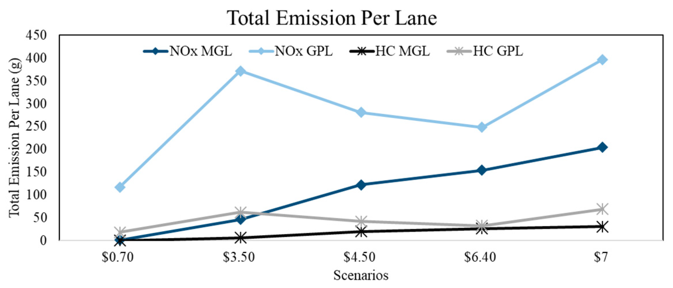
| 0.7 USD | Free (0.7 USD) | 3.5 USD | Free (3.5 USD) | 4.5 USD | Free (4.5 USD) | 6.4 USD | Free (6.4 USD) | 7 USD | Free (7.0 USD) | |
| Total Emission (g) | 2.35 | 586.9 | 935 | 1859 | 245 | 1405 | 309 | 1243 | 409.1 | 1985 |
| Emission Per Lane (g) | 1.18 | 117.4 | 46.62 | 371.9 | 122.5 | 280.9 | 154.5 | 248.7 | 204.6 | 397.1 |
| HC Emission | ||||||||||
| Scenarios | 1 | 2 | 3 | 4 | 5 | |||||
| 0.7 USD | Free (0.7 USD) | 3.5 USD | Free (3.5 USD) | 4.5 USD | 0.7 USD | Free (0.7 USD) | 3.5 USD | Free (3.5 USD) | 4.5 USD | |
| Total Emission (g) | 0.34 | 91.7 | 12.72 | 311.9 | 40.97 | 209.6 | 53.33 | 163.9 | 61.55 | 345.3 |
| Emission Per Lane (g) | 0.17 | 18.34 | 6.36 | 62.39 | 20.48 | 41.92 | 26.67 | 32.78 | 30.77 | 69.06 |
| Lane Specification | Rush Hour Periods | ||||||||||
|---|---|---|---|---|---|---|---|---|---|---|---|
| 6:00–7:00 a.m. EB | 7:00–8:00 a.m. EB | 8:00–9:00 a.m. EB | 9:00–10:00 a.m. EB | 3:00–4:00 p.m. WB | 4:00–5:00 p.m. WB | 5:00–6:00 p.m. WB | 6:00–7:00 p.m. WB | Non-Rush Hours | Daily Total EB | Daily Total WB | |
| ML Total NOx (grams/Lane) | 1287 | 1110 | 817.9 | 260.2 | 350.0 | 922.6 | 951.6 | 557.4 | 8.820 | 3651 (42% of GPL) | 2958 (32.7% of GPL) |
| GPL Total NOx (grams/Lane) | 1254 | 1164 | 1058 | 1244 | 1294 | 1339 | 1178 | 1188 | 202.3 | 8765 | 9044 |
| ML Total HC (grams/Lane) | 215.1 | 166.9 | 141.2 | 35.50 | 58.53 | 138.8 | 143.2 | 93.21 | 1.270 | 584.2 (42.6% of GPL ) | 459.1 (31.9% of GPL ) |
| GPL Total HC (grams/Lane) | 187.1 | 202.5 | 139.4 | 208.7 | 193.1 | 232.9 | 204.9 | 177.2 | 31.60 | 1370 | 1440 |
Publisher’s Note: MDPI stays neutral with regard to jurisdictional claims in published maps and institutional affiliations. |
© 2021 by the authors. Licensee MDPI, Basel, Switzerland. This article is an open access article distributed under the terms and conditions of the Creative Commons Attribution (CC BY) license (https://creativecommons.org/licenses/by/4.0/).
Share and Cite
Du, J.; Qiao, F.; Yu, L.; Lv, Y. Impact of Managed-Lane Pricing Strategies on Vehicle-Sourced NOx and HC Emissions. Gases 2021, 1, 117-132. https://doi.org/10.3390/gases1020010
Du J, Qiao F, Yu L, Lv Y. Impact of Managed-Lane Pricing Strategies on Vehicle-Sourced NOx and HC Emissions. Gases. 2021; 1(2):117-132. https://doi.org/10.3390/gases1020010
Chicago/Turabian StyleDu, Jianbang, Fengxiang Qiao, Lei Yu, and Ying Lv. 2021. "Impact of Managed-Lane Pricing Strategies on Vehicle-Sourced NOx and HC Emissions" Gases 1, no. 2: 117-132. https://doi.org/10.3390/gases1020010