Impact of Climate Variability on Rainfall Characteristics in the Semi-Arid Shashe Catchment (Botswana) from 1981–2050

Abstract

Futuristic rainfall projections are used in scale and various climate impact assessments. However, the influence of climate variability on spatial distribution patterns and characteristics of rainfall at the local level, especially in semi-arid catchments that are highly variable and are not well explored. In this study, we explore the influence of climate variability on the spatial distribution and rainfall characteristics at a local scale in the semi-arid Shashe catchment, Northeastern Botswana. The LARS-WG, Long Ashton Research Station Weather Generator downscaling method, three representative scenarios (RCP 2.6, RCP 4.5, and RCP 4.5), three trend detection methods (Mann-Kendall, Sen’s slope, and innovative trend analysis) and L-moment method were used to assess climate change impacts on rainfall. Two data sets were used; one with 40 years of observed data from 1981–2020 and the other with 70 years from 1981–2050 (40 years of observed and 30 years of projected data from 2021–2050). Generally, the study found trend inconsistencies for all the trend detection methods. In most cases, Sen’s Slope has a high estimate of observed and RCP 2.6, while ITA overestimates rainfall totals under RCP 4.5 and RCP 8.5. The trend is increasing for annual total rainfall in most gauging stations while decreasing for annual maximum rainfall. The catchment is homogeneous, and Generalized Logistic distribution is the dataset’s best-fit distribution. Spatial coverage of a 100-year rainfall between 151–180 mm will be 81% based on observed data and 87% based on projected data under RCP 2.6 scenario when it happens. A 200-year rainfall between 196–240 mm under RCP 4.5 and 8.5 has high spatial areal coverage, at least 90% of the total catchment. The outcomes of this study will provide insightful information for water resource management and flood risk assessment under climate change. There is a need, however, to assess the transferability of this approach to other catchments in the country and assess the performance of other advanced modelling systems, such as machine learning, in this region.

1. Introduction

Climate variability due to climate change worldwide has primarily been responsible for generating extreme weather conditions leading to floods and droughts. The current anthropogenic global warming of 1.5 °C compared to pre-industrial levels has increased the intensity, frequency, and magnitude of precipitation events [1,2,3]. Future projected warming beyond 2 °C will intensify precipitation events increasing the risk of flooding in some regions [4,5]. These, in turn, impact safe and adequate amounts of water availability [6,7,8], food production and security, soil erosion [9,10,11], the spread of wildfires [12,13,14], worsen the current efforts to climate resilience adaptation, damage to property and infrastructure [15]. Hydrometeorological disasters in Sub-Saharan Africa are fast changing. Despite much research on various aspects of floods, the world still witnesses severe floods [16,17,18,19,20,21]. Vulnerability and exposure to these disasters are driven by climate variability and land use changes due to rapid population growth and economic expansion. Infrastructural development and national disaster management strategies have not kept pace with the effects of changing land use/land cover patterns and climate variability on extreme rainfall events leading to floods. Floods are expected to intensify, threatening future generations due to changing climate and climate variations (15). Given the above, an improved understanding of the flooding problems is needed to develop adaptation measures and attain sustainable development.

According to the University of Notre Dame Global Adaptation Initiative (ND-GAIN), which ranks the country’s vulnerability to climate change, Botswana is considered a high-risk country, ranked 119 out of 181 countries [22,23,24,25]. Studies indicate that regions in the semi-arid zones are highly vulnerable and likely to be hit hard by hydro-metrological disasters by the middle of this century [26]. The rainfall in these regions is highly irregular, with high interannual variability. In addition, the Intergovernmental Panel on Climate Change (IPCC) has indicated that mid-latitude and semi-arid regions such as Botswana are more likely to experience extreme, intense, and frequent precipitation events [27,28]. Flood disasters affect 0.24% of the population every year in Botswana [29]. A study by [15] further indicates that the population of Botswana exposed to floods is likely to increase by 100% if the temperature increases by 3 °C. Therefore, Botswana is a climate risk country and located in the semi-arid region has been experiencing a rise in the number of high-intensity extraordinary rainfall events leading to floods in the recent past. The country has been subjected to major repetitive floods from 1972 to 2018, affecting over 178,000 individuals leaving 34,000 homeless, causing 43 fatalities and total damage amounting to over US$5 m (EM-DAT, https://www.emdat.be, accessed on 27 March 2023). Typically, between 2015–2019 over 7000 individuals have been affected by heavy storms and floods, causing five fatalities [30]. The 1999/2000 and 2001 yielded flood disasters amounting to over US$ 700,000 in economic damage. Even though the intensity and magnitude of flood events in Botswana are increasing, systematic historical records on disaster damage and loss that inform flood risk assessment and modeling are insufficient. Therefore, it is necessary to develop decision support tools that inform flood risk assessment and aid in developing cost-effective adaptive strategies to reduce the impacts of hazardous floods. These decision support tools include trend detection and the development of rainfall quantile maps which will inform the current and futuristic impact of climate variability in catchments, hence this study.

Trend detection, identification and evaluation are necessary for hydro-meteorological datasets for determining inconsistencies and fluctuations in hydrometeorological series [31]. This information gives insight into the behavior of hydro-climatological systems and is valuable in climate research [32], water resource planning, management, and decision-making. Trend analysis is commonly applied in stationarity and nonstationary detection of hydro metrological variables. Increasing and decreasing trends are warning indicators of a shifting system (climate change) [33]. To understand and explore the system dynamics, these trends must be quantified. Statistical and hydro-climatological models are essential for trend and variability detection [34]. Various trend detection techniques are available in the literature. However, Mann–Kendall (MK), Spearman Rho, and Sen’s Slope are the most frequently used. These trend detection and quantification using different methods have been studied and applied at global and regional scales in hydro-climatological variables time series [34,35], such as rainfall and temperature [36] in Northern Togo, [37] in Udaipur district of Rajasthan state (India), [38] in the Northeastern United States, [39] at a river basin of Orissa near the coastal region, [40] in Iraq, [41] at Konya Closed Basin in Turkey, [42] in the arid region of Pakistan, drought analysis in Botswana [43], streamflow [34], groundwater and water quality. Studies revealed that Mann–Kendall produces results similar to Spearman Rho [41].

A recent innovative trend analysis (ITA) method by [44,45,46] has been gaining popularity in hydro metrological studies. Unlike Mann–Kendall (MK), the ITA method has no restrictive assumptions such as serial correlations, normality and sample data. It also gives a more detailed interpretation by identifying trends in low, medium, and high values [47]. The method has been applied by [48] alongside Sen’s Slope and Mann–Kendall (MMK) methodologies to identify trends in precipitation in the Assam region of India. It has been applied in streamflow analysis with Mann Kendall (MK) and Sen’s method [49], trends detection for annual, autumn, winter, spring, and summer season rains in England [50], for annual and seasonal precipitation in Ningxia, China [51], and assessment of meteorological drought in Northwest of Algeria [52]. The ITA method also has limitations and has been criticized by [53] for its inconsistencies in mathematical formulation and contradicting basic principles of statistical inferences, making it equivalent to classical trend analysis methods once the inconsistencies are addressed.

Given the complexity of semi-arid catchments, the convective nature and high rainfall variability in semi-arid regions make it difficult for these catchments to be adequately represented by course resolution climate and hydro-climatological models [3]. These regions have been considered climate uncertainty hotspots, therefore, need special attention. However, detecting future trends, integrating climate projections in regional frequency analysis, and mapping the rate of change in rainfall distribution under different climate scenarios is not yet fully exploited in the literature.

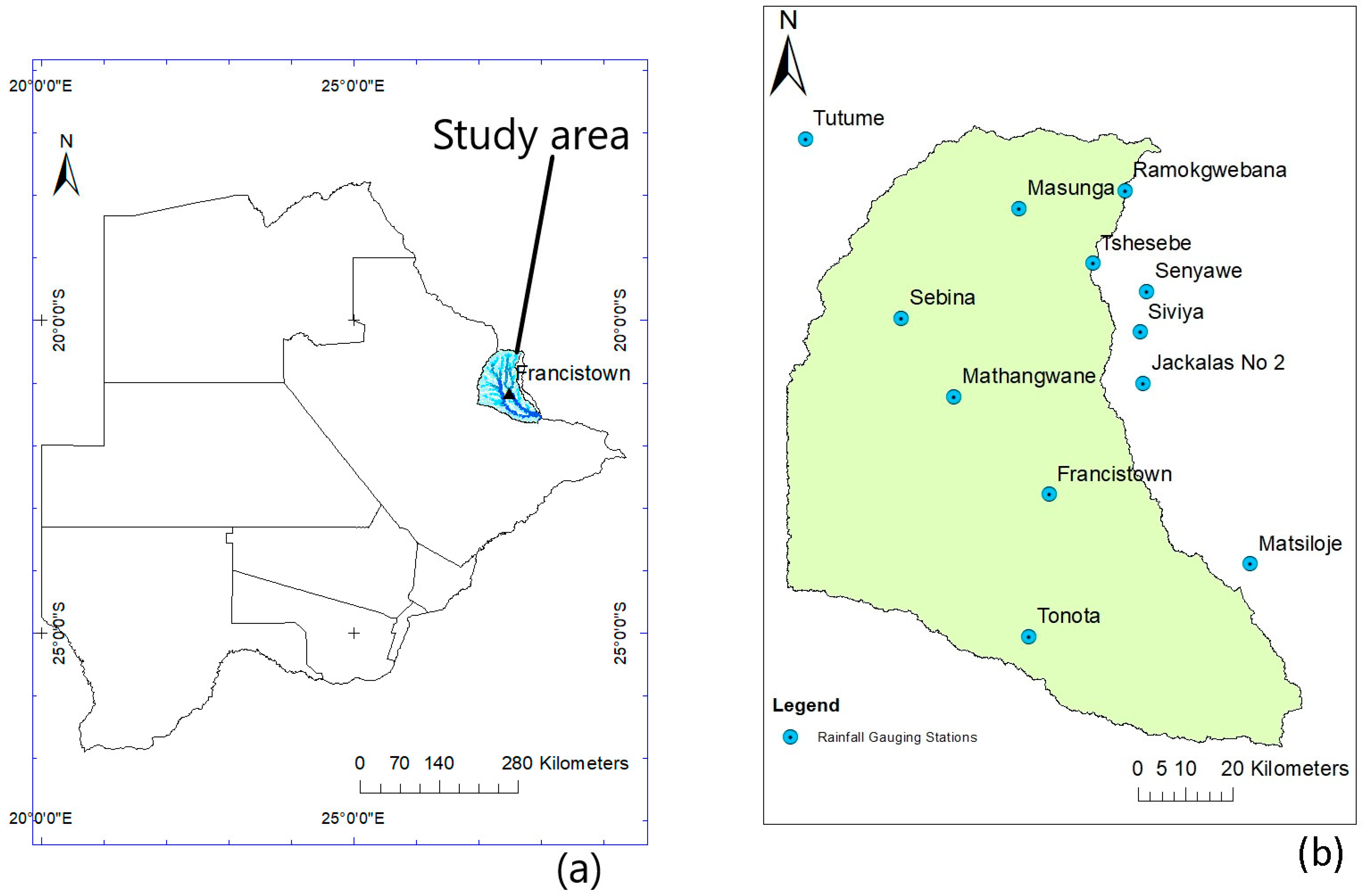
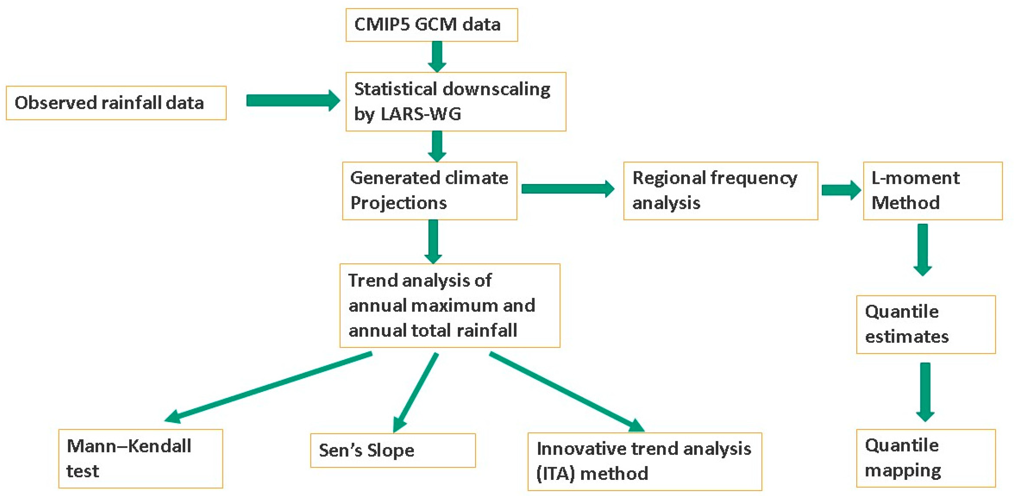
In addition to the above, the northeastern region of Botswana, Shashe catchment, which has been experiencing high rates of floods, has been identified as a suitable study area. This study aims to investigate the characteristics of rainfall to get an insight into what has changed in the past and possible future expectations. This aim will be achieved through the following objectives: (i) To project future rainfall for the Shashe catchment under Representative Concertation Pathways (RCP) 2.6, 4.5, and 8.5 using Long Ashton Research Station Weather Generator (LARS-WG) [54] from 2021–2050, (ii) To detect trends using Mann–Kendall together with Sen’s Slope and innovative trend analysis (ITA) method in observed and projected annual maximum and annual total rainfall data, and (iii) To estimate the quantiles of annual maximum rainfall and its spatiotemporal variability under both historical and projected scenarios.

2. Materials and Methods

2.1. Study Area

The Shashe River catchment is located in the northeastern part of Botswana between the longitude 27° E–28° E and latitude 20° E–22° E. Administratively, a major part of the catchment is in the northeast district with some parts in the central district as shown in Figure 1a below.

2.2. Study Area Description

The catchment has great significance economically. The catchment is home to the second largest city in the country, Francistown. This city has been considered a business hub for the country and is surrounded by Tati Nickel Mines. Rapid urbanization and rural-urban migration have given birth to urban sprawls such as the Tati Siding, Gerald Estates, Borolong and Shashemooke. The population in the catchment has been steadily increasing since the gold rush in 1900 along the Tati River to over two hundred thousand, about 10% of the country’s population. The area is also subjected to a high influx of illegal immigrants from neighbouring Zimbabwe increasing the population and resource demands. The study area is also considered the gateway to the north as it connects the northern countries such as Zimbabwe, Zambia, and Namibia with the southern part of the country and South Africa.

Hydrologically, the catchment is the source of major rivers in the country that feeds significant reservoirs. These reservoirs are the primary source of freshwater supply for the country. In addition, Dikgatlhong and Shashe Dam are connected to the southern part of the country through the North-South Water Carrier to supply significant towns and villages down south, including the capital city and surrounding villages. Ntimbale Dam, on the other hand, is the water source for the northeastern part of the country.

The catchment has a semi-arid climate with hot summers and cold winters. The dry season ranges between April and October, with high temperatures reaching 41.1 °C and minimum average temperature of 8 °C. Rainfall is unimodal, normally occurring between November and April, and it is the highest in February and March. The area is positioned close to the Intertropical Convergence Zone (ITCZ), which plays an important role in the distribution of rainfall in the Northeastern part of Botswana. The rain is characterised by high intensity for a short duration of time. The spatial distribution of the rainfall ranges between 600 mm in the northern part and 400 mm per year in the southern part of the catchment causing severe floods in the region and resulting in economic damage and displacement. Over the past decade, the Shashe catchment has been experiencing repetitive severe floods. Most of these floods occur between January and February. Floods in Botswana are mainly driven by heavy rains that arise from cascading effects of tropical cyclones from the Southwest Indian Ocean during summer advancing through the mainland of Mozambique. These cyclones bring high-intensity rainfall within a short period, thereby causing floods.

Continuous rainfall that occurred on 8 December 2004 with a magnitude of 171 mm left thousands of people homeless in Francistown in the floodplains of Tati River, affecting residents of Block-Four, Block-Seven, Block-Nine, Block-10, Riverside, Satellite, and other areas. According to the Botswana Red Cross Society (BRCS), heavy rainfall caused floods in the Tutume Sub District, Tonota Sub District, and some parts of the Northeast District in January 2013. This flood affected 842 families (about 4210 individuals) [55]. Tropical Cyclone Dineo induced floods from 13–17 February 2017 with rainfall magnitudes over 270 mm [56] overtopped bridges, leaving thousands homeless and destroying properties and fields. In February 2000, rainfall with a magnitude over 370 mm down poured continuously for three days, wiping away bridges, railroads, crops, and homesteads, leaving thousands of people homeless. The 1986 Francistown floods are also some of the catastrophic floods that claimed unquantified significant lives and caused a damaging socio-economic impact, has not been further investigated. More such disasters are anticipated to happen as climate change and variability intensifies.

The magnitude and frequency of disasters are increasing, threatening human survival and civilization, resulting in substantial economic losses. Therefore, this grey area must be researched to attain a sustainable future. Additionally, it must be given priority through the formulation of policies and strategies to facilitate disaster risk reduction.

2.3. Data Sets

Observed meteorological times series data of precipitation was acquired from the Department of Meteorological Services (DMS), ranging from 1981–2020. The records used in this study are sufficiently reliable and have been applied in similar studies. Furthermore, observations of records has been made, collected and from sources prioritising accuracy, such as the Civil Aviation Authority and metrological department. Therefore, the accuracy of the data is not questionable. The distribution of rainfall gauging stations is indicated in Figure 1b above.

Table 1. Rainfall gauging stations, their geographic location and length of record years (Source: Department of Meteorological Services (DMS), Botswana).

Station Name	Longitude	Latitude	Observed Years
Francistown	27.502515	−21.16636	1981–2020
Jackalas No 2	27.680671	−20.954196	1981–2020
Masunga	27.445115	−20.620707	1981–2020
Mathangwane	27.32	−20.98	1981–2020
Matsiloje	27.88544	−21.299711	1981–2020
Ramokgwebana	27.64629	−20.587204	1981–2020
Sebina	27.219551	−20.830506	1981–2020
Senyawe	27.688029	−20.779341	1981–2020
Siviya	27.675744	−20.857003	1981–2020
Tonota	27.463376	−21.437833	1981–2020

below gives a summary of the data used in this study.

In this research, different sets of data indicated below are required to develop a flood model. A 30-year period is the minimum recommended for climate analysis. Here we analyze extreme flood events across 40 years from 1981–2020 and into the projected future from 2021–2050 with various hydroclimatic and land use/land cover dynamics. The choice of the base period beginning in 1981 was the beginning of accelerated human influence on the climate system [27,28,57]. The flow chart describing the methodology is illustrated below in Figure 2:

2.4. Rainfall Projections

In this study, precipitation projections are statistically downscaled using Long Ashton Research Station Weather Generator (LARS-WG) under Representative Concertation Pathways (RCP) 2.6, 4.5, and 8.5 radiative forcing by applying an ensemble of 18 General Circulation Models (GCMs) from Coupled Model Inter-comparison Project Phase 5 (CMIP5) for creating data sets required for assessing impacts of climate change on extreme events. LARS-WG downscaling method was developed by [4] and has been used in several recent studies for future climate projections such as [58,59,60].

The model was proved to have high predictive capacity; therefore, it was used in this study to produce 30 years of synthetic daily scale data from 2021–2050 based on statistical characteristics of observed data by applying monthly change factor between the 18 GCMs and observed data. As a result, implementing climate mitigation measures to lower emissions by 50% by 2050 will limit warming to 2 °C above the preindustrial era [27], by 40–70% in 2050 compared to 2010 [61] and limit warming to 1.5 °C if greenhouse gasses are reduced by 40–70% in 2050 compared to baseline period (1986–2005) [62].

It applies a semi-empirical distribution model known as the cumulative probability distribution function to determine the confidence interval for data sets. Daily data for a given station for the baseline period is input into the model to determine parameters for probability distributions. Weather sequence of the same statistical properties as the observed data is generated using suitable distributions. The method was adopted for its advantages over other models, including its statistical nature, improvements in the spatial accuracy of GCMs, simplicity, modest data requirement, efficiency, and cost-effectiveness. It can downscale daily time series data directly applied to hydrological and land use models. In addition, statistical models have a higher degree of accuracy and computational speed than other models. The models have been applied in several studies, such as [59,60].

To assess the performance of the LARS-WG model, Chi-square, t-test, and f-test statistics were used. The chi-square test compares observed and synthetically generated data to check if they come from the same probability distribution. The t-test mean values of the observed and simulated data to assess if they come from the same population, while f-test statistic determines if the observed and synthetic data are from the normal distributions with the same variance. All these tests have a p-value used to accept or reject the hypothesis of whether the observed and generated data comes from the same distribution. The total annual and annual maximum values are then extracted and characterized.

2.5. Trend Analysis

In the present study, Mann–Kendall (MK) [63,64] is a rank-based non-parametric statistical test commonly used to determine if a monotonic upward or downward trend exists within the data of interest over a period employed. For comparative purposes, Mann–Kendall, with Sen’s Slope and innovative trend analysis method, will be applied in this study to detect the trend and magnitude of trends in rainfall data.

2.5.1. Mann-Kendall Test

Mann-Kendall (MK) is a non-parametric test method commonly used in detecting trends in data. The advantage of Mann-Kendall is that it is less sensitive to inhomogeneous time series and can overcome the challenge of data skewness. Mann-Kendall is an exploratory analysis measure to indicate any significant change in data. The robustness of MK has an advantage in dealing with data that is not normally distributed, missing data values, and tolerating outliers and censored data, which are common challenges associated with hydro-climatological data. The Modified Mann Kendall (MMK) is modified by incorporating pre-whitening to remove serial correlation in data sets. Rainfall is less likely to be affected by serial correlations; hence the Mann-Kendall method is sufficient for application in this study. The Mann-Kendall S Statistic is determined by:

$$S={\displaystyle \sum }_{k-1}^{n-1}{\displaystyle \sum }_{j=k+1}^{n}sgn\left(x_j-x_k\right)$$

(1)

$$sgn\left(x_j-x_k\right)=\left\{\begin{array}{rrrr}+1& if& \left(x_j-x_k\right)& >0\\ 0& if& \left(x_j-x_k\right)& =0\\ -1& if& \left(x_j-x_k\right)& <0\end{array}\right.$$

(2)

where x_j and x_i are annual values in years j and i, j > i, respectively. The ordered time series from i = 1, 2, ………n − 1 and x_j, which is ranked from j = I + 1, 2, ………. n is evaluated by comparing subsequent data values. When the current time data value is higher than the data value of the previous period, the S statistical value is increased by 1. Contrariwise, S value is decreased by 1. According to [63,64] is normally distributed when n ≥ 8 having mean:

$$E\left(S\right)=0$$

and variance statistic is given as

$$V\left(S\right)=\frac{n \left(n-1\right) \left(2n+5\right)-{\sum }_{i=1}^m{T}_i\mathrm{i}\left(\mathrm{i} -1\right)\left(2\mathrm{i} +5\right)}{18}$$

(3)

where T_i is the amount of data in the tied group, and m is the number of groups of tied ranks. The Mann-Kendall standardized test statistic Z is computed by:

$$Z=\left\{\begin{array}{cc}\frac{\left(S-1\right)}{\sqrt{Var\left(s\right)}}\hfill & if S>0\hfill \\ \hfill 0\hfill & if S=0\\ \frac{\left(S+1\right)}{\sqrt{Var\left(S\right)}}\hfill & if S<0\hfill \end{array}\right.$$

(4)

where Z is statistical of the test, sgn is the signum function, x is the hydrological variable, n is the historical series length, and j and k are time indices. The Mann-Kendell standardized test statistic Z has a mean E(Z) = 0 and V(Z) = 1.

The null hypothesis indicating no trend in the data must be accepted if the absolute value |Z| ≤ Z_1−α/2 at a significance level α [65].

H₀ (null hypothesis).

Assumes no trend is present. The data is random and independent.

H_A (alternative hypothesis).

Assumes a trend is present in the data, either a positive or negative trend.

For a significance level of 5%, the Z-value Z_α/2, 0.025 is 1.96. That is, if |Z| is less than 1.96, the trend is invalid; therefore, reject the null hypothesis.

A commonly applied 5% significance level for the p-value has been adopted for this study. As a result, if the p-value of the test is lower than 0.05, then there is statistically significant evidence that a trend is present in the time series data. The rainfall data of all the gauging stations were tested at a 95% confidence interval.

2.5.2. Sen’s Slope Estimator

The magnitude of the trend or true slope (change per unit time) is estimated by a robust Sen’s slope estimator β established [66]. Sen’s method calculates both the slope and the intercept. This method has no prior assumptions, can be shown in both monotonic or non-monotonic form and has been applied successfully in hydrometeorological time series. The slope is formulated as follows:

$$\mathsf{\beta }=\mathrm{median}\left(\frac{x_j-x_i}{j-i}\right) j>i$$

(5)

when the β is negative, the trend is downward (values decrease over time), while a positive β indicates an upward trend.

2.5.3. Innovative Trend Analysis (ITA) Method

The innovative Trend Analysis (ITA) method is a trend detection method developed by [44,45]. This approach, unlike MK, does not have any restriction on the normality, sample size and serial independence. The method is based on a 1:1 (45°) scatter plot of time series points split into two halves on a Cartesian coordinate system. Each time series is arranged in ascending order. The first series is plotted horizontally (X), and the second is vertical (Y). Any deviation of scatter plots from the 1:1 line indicates the presence of a trend, and the closer the plots are to the line, the smaller the trend magnitude. According to Şen [45], if the scattering points are below the 1:1 line, the trend decreases, while points above the 1:1 line indicate an increasing trend. The details of the methodology are explained below.

(i)

the x₁, x₂, x₃, … x_n time series is split into two halves, {S_(1,2/2)} and {S_(1,2/2)}.

$$S_{1,\frac{n}{2}}=\left\{x_1, x_1, x_1 \dots , x_{\frac{n}{2}}\right\}$$

(6)

$$\left\{S_{2,\frac{n}{2}}\right\}=\{x_{\frac{n}{2}+1}, x_{\frac{n}{2}+2}, x_1 \dots , x_n\}$$

(7)

(ii)

Sort elements of each series from the smallest to the largest

$$\left\{t_1\right\}=\left\{min\left(s_{1,n/2}\right),\dots , s_{1 },\dots max\left(s_{1,n/2}\right)\right\}(1<i<n/2)$$

(8)

$$\left\{t_2\right\}=\left\{min\left(s_{2,n/2}\right),\dots , s_{1 },\dots max\left(s_{2,n/2}\right)\right\}(1<j<n/2)$$

(9)

(iii)

The slope of the trend is then calculated using [46]:

$$s=\frac{2\left({\overline{y}}_2-{\overline{y}}_1\right)}{n}$$

(10)

where s is the trend slope, $-{\overline{y}}_1$ and ${\overline{y}}_2$ are the arithmetic averages of the first and second series while n is the amount of data.

2.6. L-Moments—Regional Frequency Analysis

Frequency analysis estimates the magnitude of extreme events and the frequency at which they occur. This entails fitting maximum hydroclimatic data to a probability distribution to estimate the peak of a given return period [67]. Reliable estimation of extreme events is necessary for proper planning and design of civil and hydraulic structures, flood risk management, water resource management and planning, and probability mapping. Since extreme events are random physical processes prone to uncertainties, these uncertainties are quantified by statistical techniques. Frequency analysis requires the selection of a robust probability distribution and parameter estimation method. Various research has been done on different parameter estimation methods. These methods include the maximum likelihood method, the method of moments, probability-weighted moments (PWMs) [68], the least squares method, mixed moments, maximum entropy, the generalized method of moments and the incomplete means method.

The L-moments are a combination of linear probability-weighted moments (PWMs) defined by [68,69,70], demonstrating that L-moments can dictate homogeneous regions, select the most suitable regional frequency distribution, and estimate extreme quantiles at the region of interest. The development of L-moment is the most remarkable contribution to statistical hydrology. It is the most widely used approach in RFA and has been credited for its superior performance and statistical characteristics, just to mention a few [16,18,65,67,69,71,72,73,74,75,76,77,78] Th.is approach has been adopted for this study for its robustness as they tend to suffer less effects of sampling variability, requires less computational power, they are more robust in the presence of outliers. Furthermore, they yield more efficient parameter estimates than the maximum. Furthermore, l-moments are preferable to other conventional moments because they can analyze a wide range of distributions [69].

Lineal moments (L-moments) describe the shape of frequency distributions. [79] defined the first four L-Moments λ₁, λ₂, λ₃ and λ₄ are L-moments of probability weighted moments as:

$${\lambda }_1=E\left(X_{1:1}\right)$$

(11)

$${\lambda }_2=1/2E\left(X_{2:2 }-X_{1:2}\right)$$

(12)

$${\lambda }_3=1/3E\left(X_{3:3}-2X_{2:3}+X_{1:3}\right)$$

(13)

$${\lambda }_4=1/4E\left(X_{4:4}-3X{ }_{3:4}+3X_{3:4}+X_{1:4}\right)$$

(14)

where λ₁, λ₂, λ₃ and λ₄ represent the parameters related to location, scale, shape and peakedness, respectively. The most useful quantities for summarizing probability distributions of the L-moments are location (λ₁), and scale (λ₂), which are used to define L-moment ratios as [79]:

$${\tau }_2={\lambda }_2/{\lambda }_1$$

(15)

$${\tau }_3={\lambda }_3/{\lambda }_2$$

(16)

$${\tau }_4={\lambda }_4/{\lambda }_2$$

(17)

The ranges of L-CV (coefficient of L-variation, τ₂), L-skewness (τ₃) and L-kurtosis (τ₄) are given as 0 ≤ τ₂ < 1, −1 < τ₃ < 1 and −1 < τ₄ < 1 respectively.

2.6.1. Discordancy and Heterogeneity Measure

• Discordancy measure

Regional frequency analysis using the L-moments test for outliers, trends, incorrect data values and shifts by comparing L-moment statistic ratios for different gauging sites (69). This method combines L-moment ratios into a single statistic and then measures its discordancy against the average L-moment ratios of a group of similar sites. The ratios can identify discordant data by detecting errors, outliers, and heterogeneities in sample data. The L-CV (or τ), the L-Skewness (or τ₃), and the L-Kurtosis (or τ₄) are the three L-moment statistic ratios used to measure discordancy in a data sample. Their sample estimates are denoted by t, t₃, and t₄. In a group of sites, L-moments identifies those sites that are inconsistent or in agreement with the whole group. The discordancy measure is defined by [69] as:

$$D_i=\frac{1}{3}N{\left(u_i-ū\right)}^T{A}^{-1}\left(u_i-ū\right), i=1, 2,\dots , N$$

(18)

D_i is the discordancy measure for site i, N is the number of sites in the group, superscript T is the transposition of a vector or matrix, u_i is a vector containing the $t^{\left(i\right)}, t_3{}^{\left(i\right)}\mathrm{and} t_4{}^{\left(i\right)}$ values denoting coefficients of variation, skewness, and kurtosis, respectively in a 3-dimension space for site i. The 3 × 1 vector u_i is expressed as:

$$u_i={\left(t^{\left(i\right)}, t_3{}^{\left(i\right)}, t_4{}^{\left(i\right)}\right)}^T$$

(19)

The unweighted group average is defined by the following:

$$ū=N^{-1}{\displaystyle \sum }_{i=1}^N{u}_i={\left(t^{\left(R\right)}, t_3{}^{\left(R\right)}, t_4{}^{\left(R\right)}\right)}^T$$

(20)

where N is the number of gauging stations in the region R. A defines the matrix of sums of squares and cross-products:

$$A={\displaystyle \sum }_{i=1}^N(u_i-ū){(u_i-ū)}^T$$

(21)

A site can be regarded as discordant if the D_i value exceeds the critical value D_crit, which depends on N, the number of sites within region R. [69] has noted that for N = 10, the discordant value should not exceed 2.491.

• Heterogeneity measure

L-moment ratios generally group the sites of interest and measure “what would be expected of a homogeneous region” [69]. The dispersion of the at-site L-moment ratios was attained by plotting them on graphs of L-skewness versus L-CV and L-skewness versus L-kurtosis. Simulation is used to establish what would be expected using a selected distribution model. The robust Kappa distribution model has been selected to perform the simulations since it can represent generalized logistic, generalized extreme-value, and generalized Pareto distributions as recommended by [69]. Its parameters are ξ, α, k, and h, with density, cumulative distribution, and quantile functions defined below:

If a region of interest has N sites with the site i having record length n_i and sample L-moment ratios denoted by t⁽ⁱ⁾, t₃⁽ⁱ⁾, and t₄⁽ⁱ⁾. The regional average L-CV, L-skewness, and L-kurtosis is denoted by t^R, t₃^R, and t₄^R. The weighted proportionally is then defined by [69]:

$$t^R={\displaystyle \sum }_{I=1}^N{n}_i{t}^{\left(i\right)}/{\displaystyle \sum }_{I=1}^N{n}_i$$

(22)

Weighted standard deviation V of the at-site sample L-CVs is for each stimulated region is calculated by:

$$V={\left\{{\displaystyle \sum }_{I=1}^N{n}_i{\left(t^{\left(i\right)}-t^R\right)}^2/{\displaystyle \sum }_{I=1}^N{n}_i\right\}}^{\frac{1}{2}}$$

(23)

Kappa frequency distribution has been fitted to regional average L-moment ratios to run many simulations N_sim for a region with N sites. The simulated homogeneous regions have the same record length and assessed in a series of Monte Carlo simulation trials [69]. From the simulations, N_sim of the weighted standard deviation V, the mean $\widehat{\mu }v$ and standard deviation $\widehat{\sigma }v$ are determined. The mean $\widehat{\mu }v$ is defined by:

$$\widehat{\mu }v=\frac{1}{N_{sim}}{\displaystyle \sum }_{l=1}^{N_{sim}}{V}_l$$

(24)

where $\widehat{\sigma }v$ is the estimated standard deviation of the N_SIM values of V_l and it is defined by:

$$\widehat{\sigma }v=\sqrt{\frac{{\sum }_{l=1}^{N_{sim}}{(V_l-\widehat{\mu }v)}^2}{N_{sim}}}$$

(25)

The heterogeneity H measure is then calculated by:

$$H=\frac{\left(V-\widehat{\mu }v\right)}{\widehat{\sigma }v}$$

(26)

A region is considered heterogeneous if H is sufficiently large. When H ≥ 2, the region is acceptably homogeneous if H < 1 and possibly heterogeneous if 1 ≤ H < 2.

2.6.2. Choice of a Frequency Distribution

Properties influencing the selection of distribution models depend on their ability to capture and replicate significant data features required in modelling. For example, the best-fit distribution is measured by a goodness-of-fit statistic considering tail weights consistent with a set of homogeneous regional data. For this reason, this study will adopt distributions with three parameters as they can yield less biased quantile estimates in the tails. As recommended by [69,80], this study will fit the following three-parameter distributions: generalized logistic (GLO), generalized extreme value (GEV), generalized Pareto (GPA), lognormal (LNO), and Pearson type III (PIII) is fitted to the regional average L-moment ratios. The goodness-of-fit test measure Z^DIST for each distribution is then expressed as:

$$Z^{DIST}=(t_4^{DIST}-t_4^R+B_4)/{\sigma }_4$$

(27)

The Z^DIST goodness-of-fit measure selects a distribution that gives the closest estimate as observed data. The best-fit model is judged by the difference between L-kurtosis $t_4^{DIST}$ of the fitted distribution and the L-kurtosis $t_4^R$ of the regional average. The standard deviation ${\sigma }_4$ of $t_4^R$ is obtained through repeated simulations of a kappa region with the same number of sites and record lengths as the observed data. The bias of the simulated region is attained from the same simulations as ${\sigma }_4$ and it is calculated by:

$$B_{4 }=N_{sim}^{-1}{\displaystyle \sum }_{m=1}^{N_{sim}}\left(t_4^{\left[m\right]}-t_4^R\right)$$

(28)

where N_sim is the number of realizations for sites with N sites and m is a simulation. The standard deviation ${\sigma }_4$ of $t_4^R$:

$${\sigma }_4={\left[{\left(N_{sim}-1\right)}^{-1}\left\{{\displaystyle \sum }_{m=1}^{N_{sim}}{\left(t_4^{\left[m\right]}-t_4^R\right)}^2-N_{sim}{B}_4^2\right\}\right]}^{\frac{1}{2}}$$

(29)

A region is considered homogeneous if $Z^{DIST}$ if it is close to zero and it is acceptable of $\left|Z^{DIST}\right|\le 1.64$. In addition to the $Z^{DIST}$ and the L-moment ratio diagram has been added to compare the statistics visually. The best-fit model with the least bias and $Z^{DIST}$ is considered for flood quantile estimation.

2.6.3. Estimation of the Quantiles

After selecting the best-fit distribution model, its standardized quantiles are estimated using regional parameters, which allows the calculation of the regional growth curve. The quantile estimates $\widehat{Q_i}\left(F\right)$ for the site i with non-exceedance probability F (0 < F < 0) is given by:

$$\widehat{Q_i}\left(F\right)={\hat{\mu }}_i\hat{q}\left(F\right)$$

(30)

where $\hat{q}\left(F\right)$ denotes the rescaled distribution, ${\widehat{\mu }}_i$ is the flood index estimate for the site i.

There is always uncertainty when dealing with statistical analysis. Therefore, the quantiles are also assessed for uncertainty before the results are helpful. The accuracy of quantiles of the estimated regional frequency distribution is estimated by Monte Carlo simulation with a simulated region with the same number of sites, record length at each site, and regional average L-moment ratios as the actual data [69].

The relative RMSE has been applied here to measure the accuracy of quantile estimate for non-exceedance probability ${\hat{Q}}_i^{\left[m\right]}\left(F\right)$ for site i at m^th repetition. Let M be the number of simulations, $Q_i\left(F\right)$ implies the true growth curve of a site i, then the relative RMSE of the estimated regional growth curve at a site i can be computed by:

$$R_i\left(F\right)={\left[M^{-1}{\displaystyle \sum }_{m-1}^M{\left\{\frac{{\hat{Q}}_i^{\left[m\right]}\left(F\right)-Q_i\left(F\right)}{Q_i\left(F\right)}\right\}}^2\right]}^{\frac{1}{2}}$$

(31)

The regional average accuracy of the estimated regional growth curve is estimated as:

$$R^R\left(F\right)=N^{-1}{\displaystyle \sum }_{i-1}^N{R}_i\left(F\right)$$

(32)

The growth curve estimate for quantile is calculated as:

$$Q_i\left(F\right)={\mu }_i{q}_i\left(F\right)$$

(33)

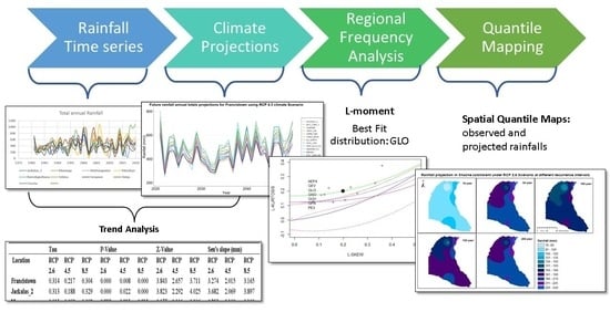
3. Results

3.1. Rainfall Projections

This study used an ensemble of eighteen General Circulation Models (GCMs) from Coupled Model Inter-comparison Project Phase 5 (CMIP5) to project rainfall in ten rainfall gauging stations distributed across the country. LARS-WG model supports ACCESS1_3, bcc-csm1-1, BNU-ESM, CanESM2, CMCC_CM, CNRM-CM5, CSIRO-Mk3-6-0, EC_EARTH, GFDL-ESM2M, HadGEM2-ES, INMCM4, IPSL-CM5A-MR, MIROC5, MIROC-ESM, MIROC-ESM-CHEM, MRI-CGCM3, NorESM1-M and NCAR_CCSM4 for Representative Concentration Pathway (RCP) 4.5 and 8.5 scenarios. Under RCP 2.6 only BCC_CSM1_1, CanESM2, CSIRO_MK36, GISS_E2_R_CC, and HadGEM2_ES are supported by LARS-WG model. Details about the model agency and the country it was developed are indicated in Appendix A 

Table A1. General Circulation Models (GCMs) from Coupled Model Inter-comparison Project Phase 5 (CMIP5) were used in rainfall projections in this study.

Model Name	Model Country	Model Agency
ACCESS1_3	Australia	Commonwealth Scientific and Industrial Research Organisation, Australia), and BOM (Bureau of Meteorology, Australia)
bcc-csm1-1	China	Beijing Climate Center, China Meteorological Administration
BNU-ESM	China	College of Global Change and Earth System Science, Beijing Normal University, China
CanESM2	Canada	Canadian Centre for Climate Modeling and Analysis
CMCC_CM	Italy	Centro Euro-Mediterraneo per I Cambiamenti Climatici
CNRM-CM5	France	National Centre of Meteorological Research, France
CSIRO-Mk3-6-0	Australia	Commonwealth Scientific and Industrial Research Organization/Queensland Climate Change Centre of Excellence, Australia
EC_EARTH	Sweden	EC-EARTH consortium
GFDL-ESM2M	USA	NOAA Geophysical Fluid Dynamics Laboratory, USA
HadGEM2-ES	United Kingdom	Met Office Hadley Center, UK
inmcm4	Russia	Institute for Numerical Mathematics, Russia
IPSL-CM5A-MR	France	Institut Pierre Simon Laplace, France
MIROC5	Japan	Atmosphere and Ocean Research Institute (The University of Tokyo), National Institute for Environmental Studies, and Japan Agency for Marine-Earth Science and Technology
MIROC-ESM	Japan	Japan Agency for Marine-Earth Science and Technology, Atmosphere and Ocean Research Institute (The University of Tokyo), and National Institute for Environmental Studies
MIROC-ESM-CHEM	Japan	Japan Agency for Marine-Earth Science and Technology, Atmosphere and Ocean Research Institute (The University of Tokyo), and National Institute for Environmental Studies
MRI-CGCM3	Japan	Meteorological Research Institute, Japan
NorESM1-M	Norway	Norwegian Climate Center, Norway
NCAR_CCSM4	USA	National Center of Atmospheric Research, USA

.

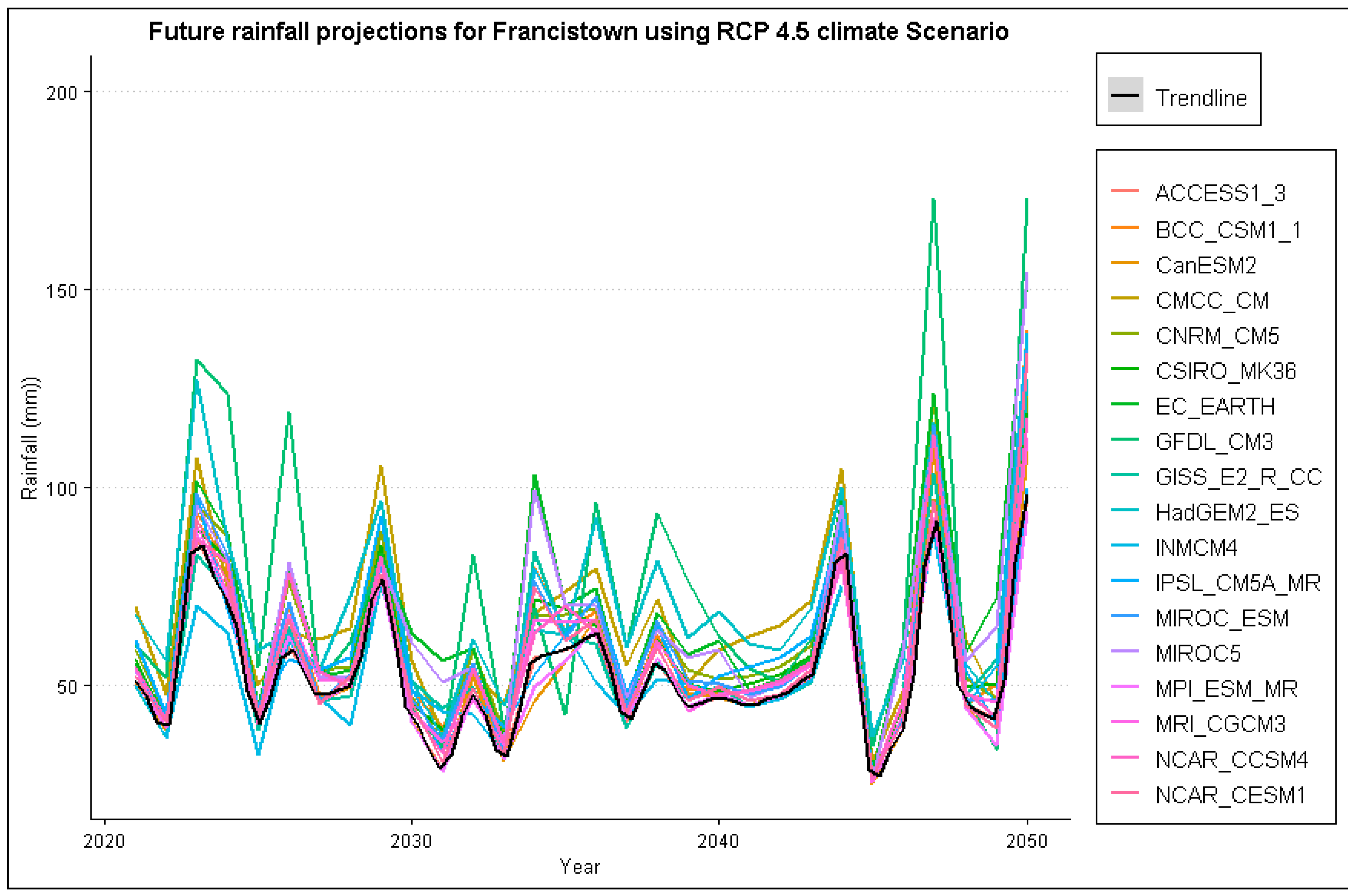
Daily rainfall projections were performed from 2021–2050, out of which annual maximum and total annual rainfall were determined under Representative Concertation Pathways (RCP) 2.6, 4.5 and 8.5 climate scenarios. This study used a non-parametric Locally estimated scatterplot smoothing (Loess) to generate the best-fit line. This method uses weighted linear regression and weighted moving average smoother to fit a smooth curve through a scatter plot without assuming that the data must fit some distribution shape.

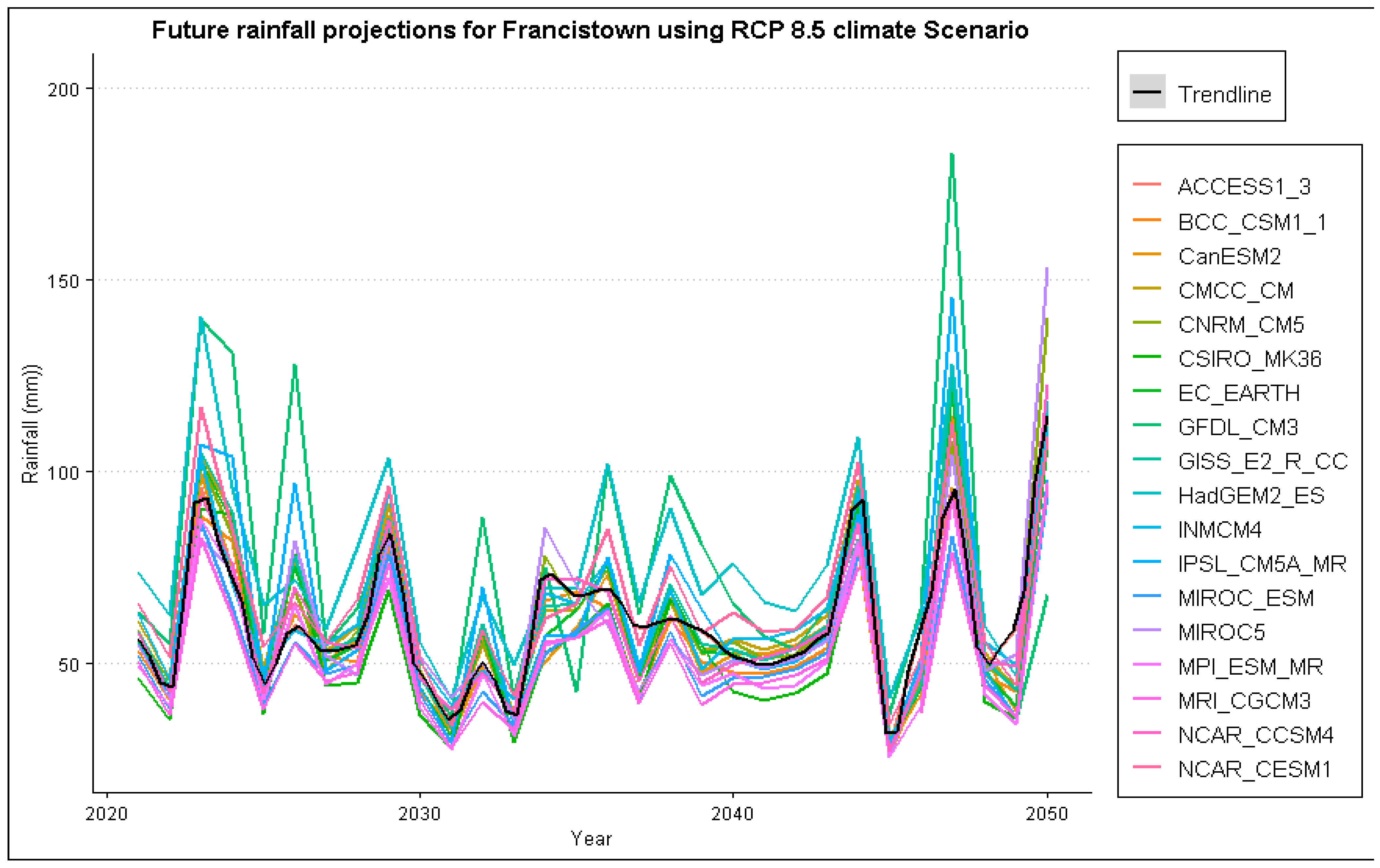
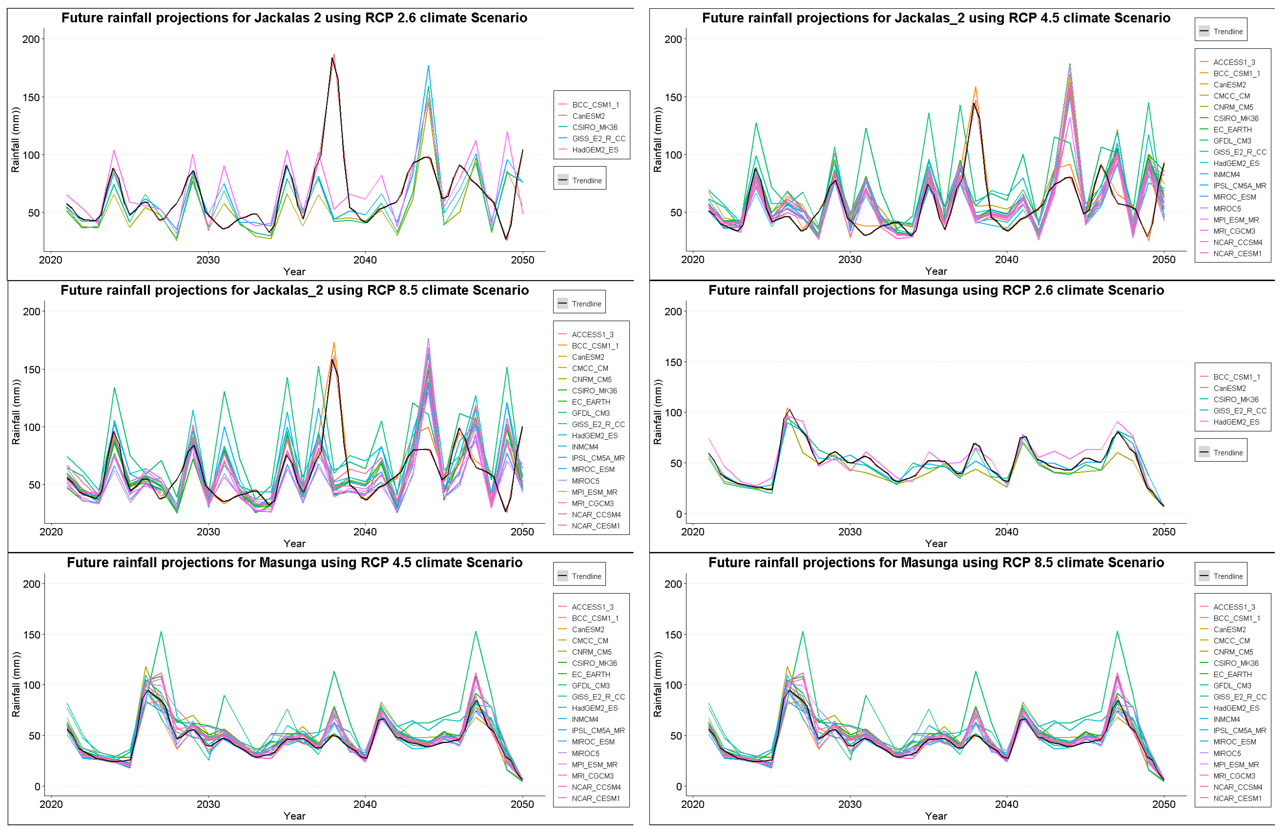
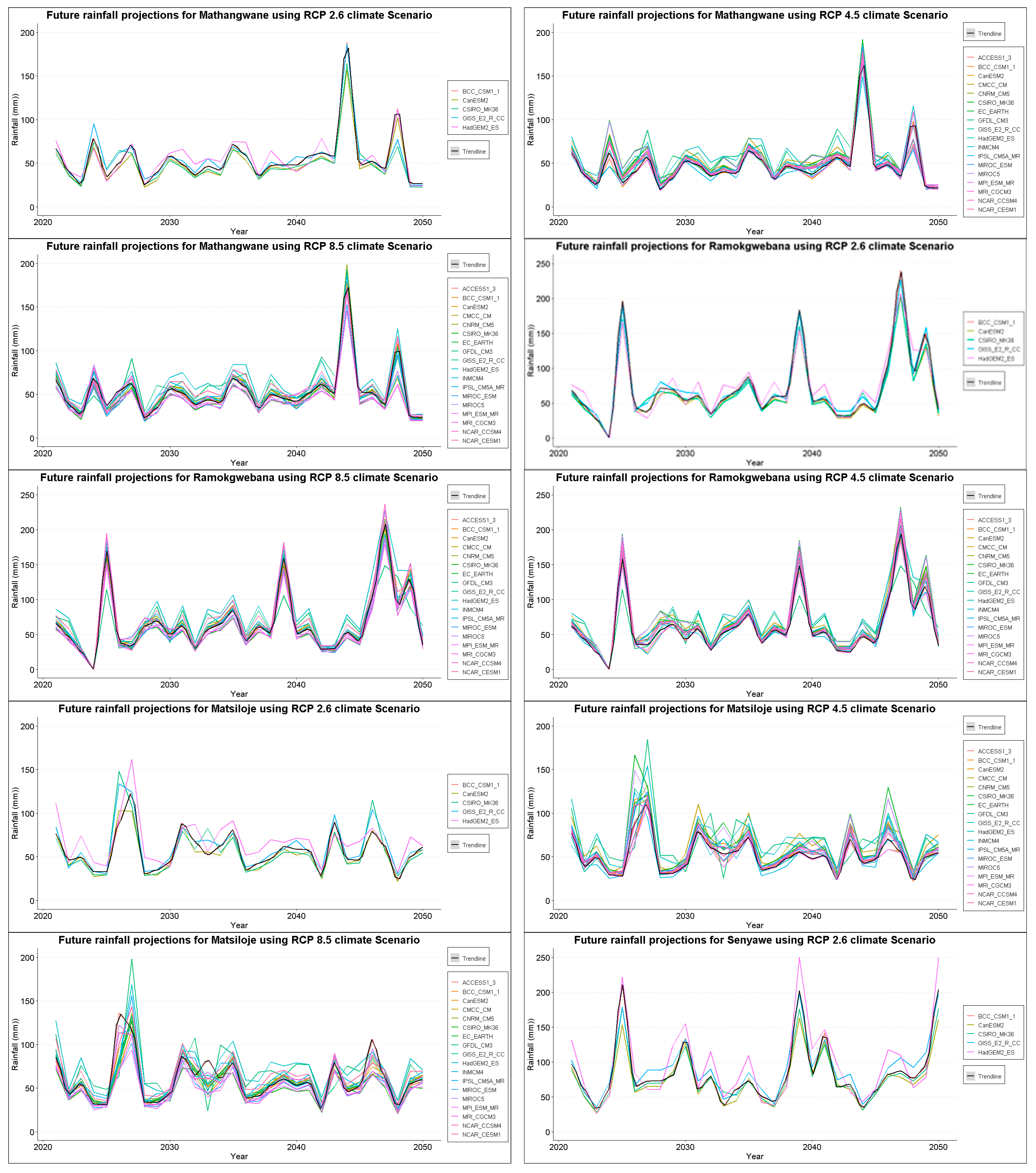
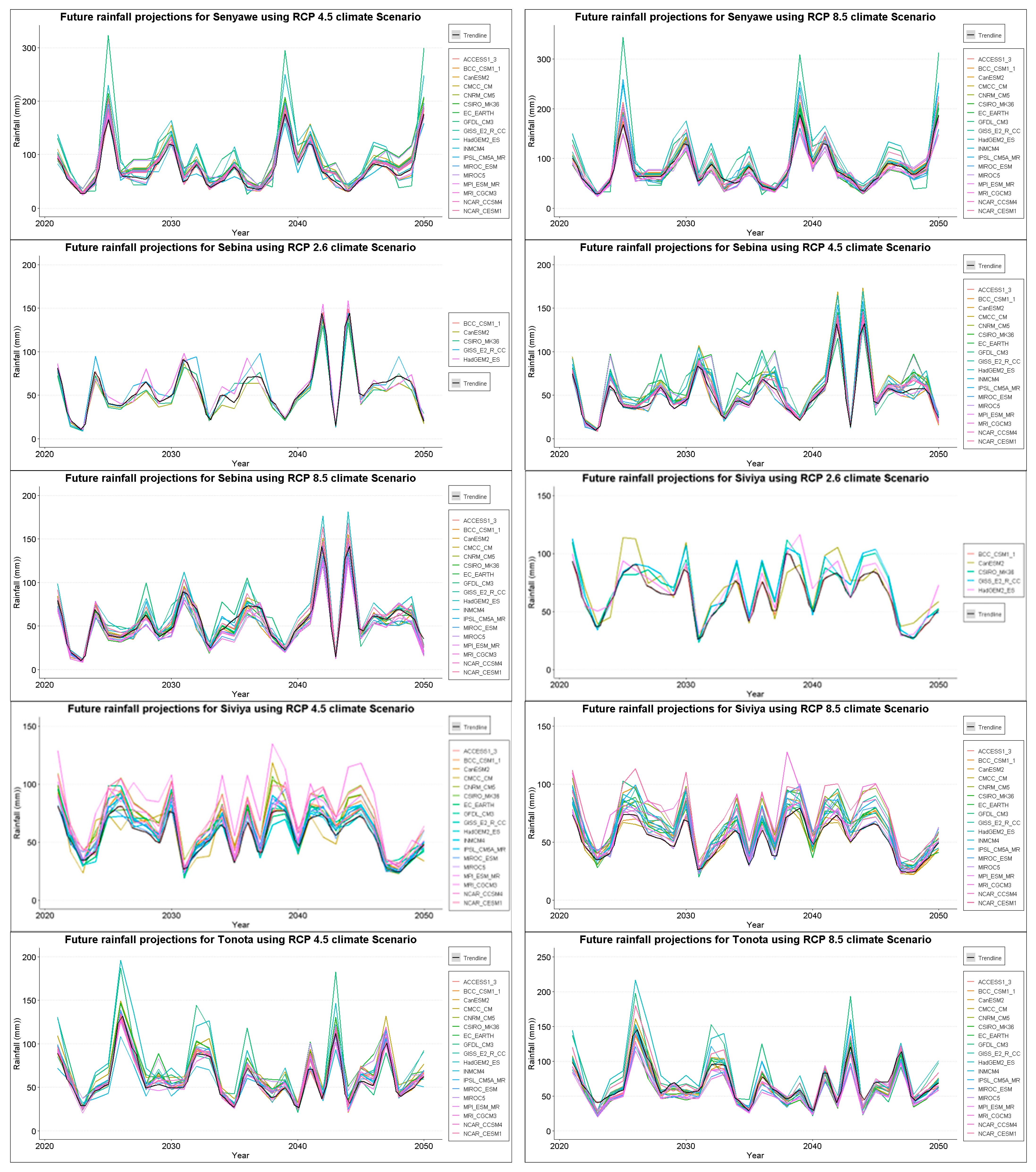
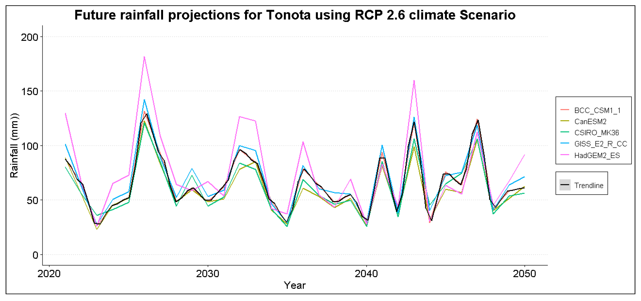
The projection for Francistown has high variability in the first ten and last ten years for all the climate scenarios reaching a maximum of 100 mm between 2040–2050. Jackalas 2 shows high rainfall projections between 2030–2040, the maximum being over 150 mm under RCP 8.5 climate scenario. Masunga shows less variability between 2025–2045, with highs of 100 mm under the RCP 2.6 climate scenario. Mathangwane also shows less variability averaging around 50 mm across all scenarios, with maximums recorded around 2045 estimated at around 175 mm. Matsiloje estimates are high in the first decade, decreasing with less variability towards 2050. The projections for Ramokgwebana, Siviya and Senyawe are high between 2040 and 2050, ranging from 100 to 200 mm. Tonota, on the other hand, is highly variable throughout, ranging between 40–150 mm. Below are samples for annual maximum plot projections for Francistown in Figure 3 and Figure 4. Other plots are in the Appendix A Figure A1 for reference purposes.

3.2. Total Annual Rainfall Projections

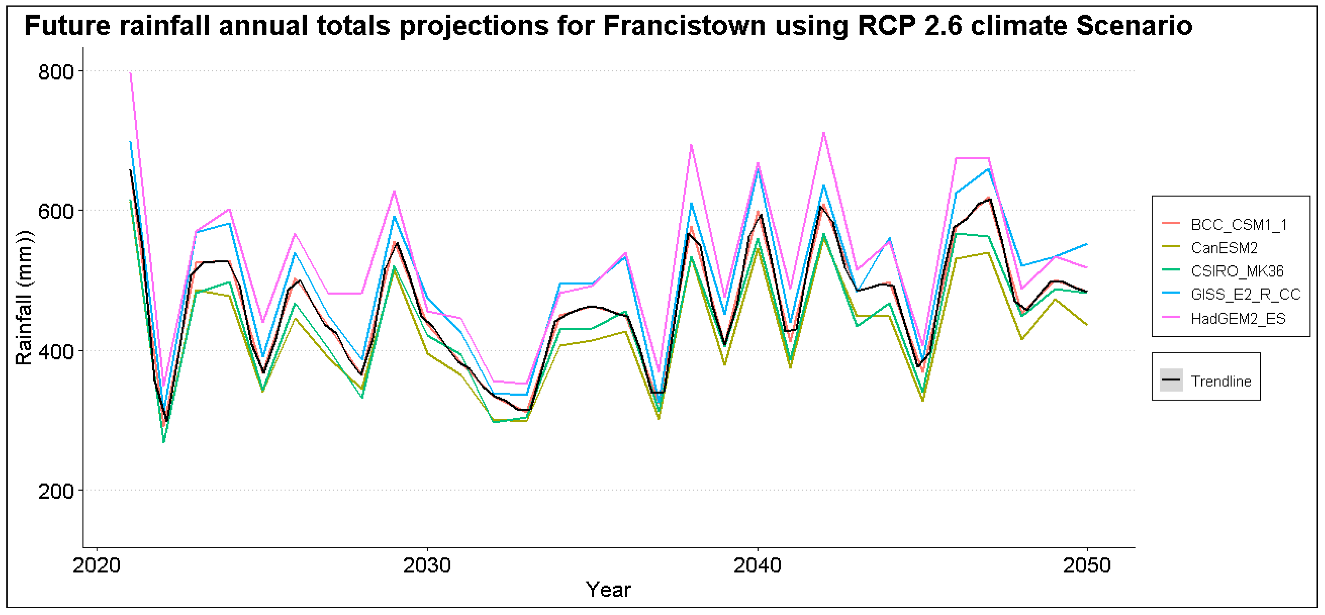
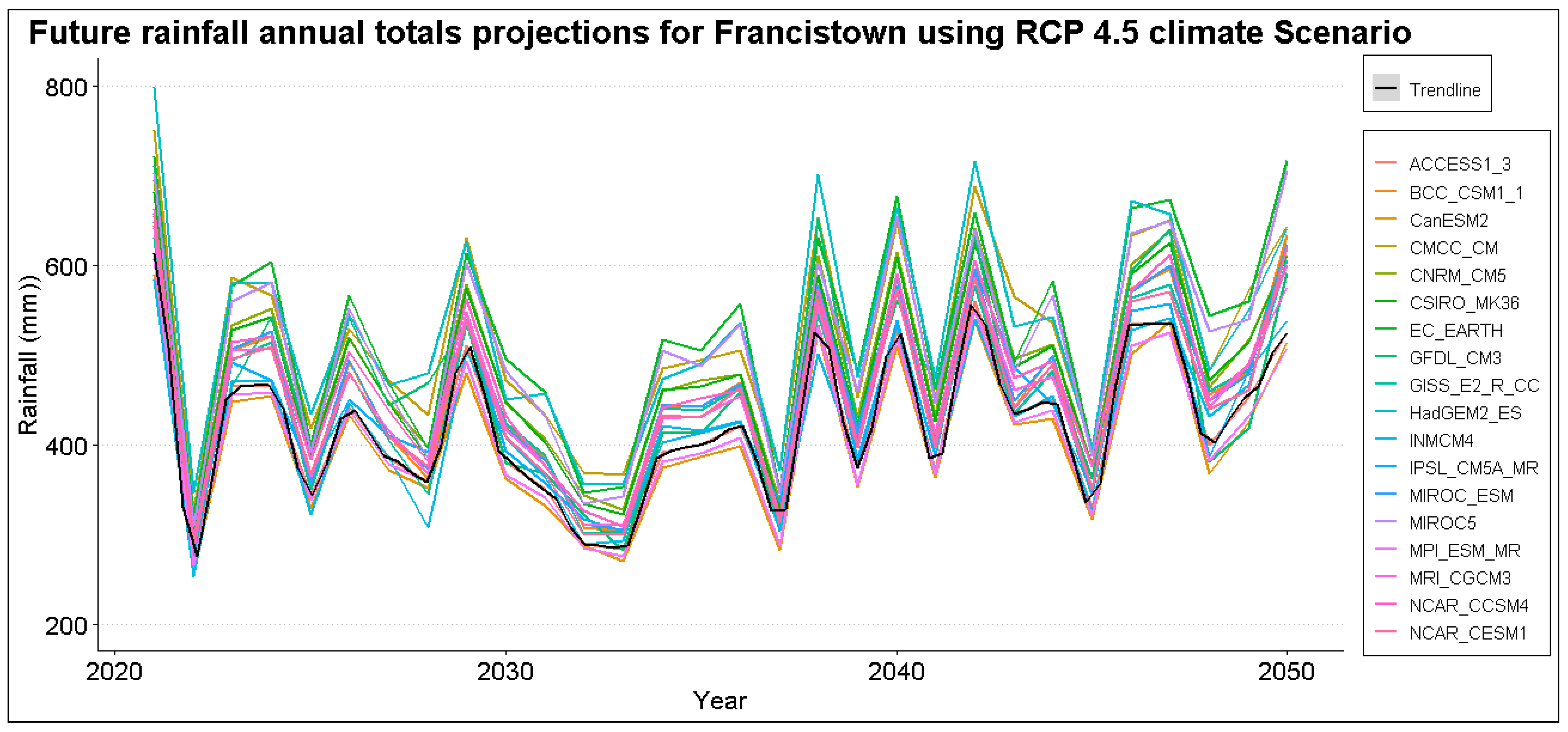
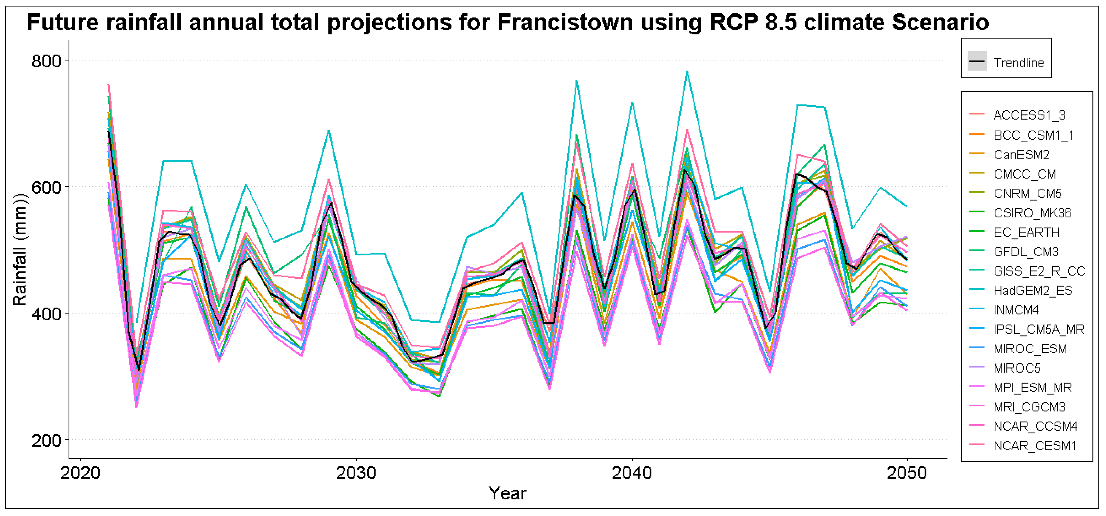
Total annual rainfall projections for Jackalas 2 are highly variable, with projections reaching a maximum of 750 mm. Masunga shows a positive increase in total annual rainfall to a maximum of 800 mm across climate scenarios. A maximum of 1000 mm is expected in Mathangwane, with high variability until 2050. Matsiloje has high projections in the first and last decade, reaching a maximum of 750 mm per year. Increasing rainfall trends are anticipated in Ramokgwebana, with a maximum of 1000 mm expected around 2040. In Sebina, high variability is anticipated between the first and last decade, while Senyawe is less variable. However, over 1600 mm is expected towards 2050. Tonota, Siviya and Francistown are highly variable with undefined patterns with annual totals averaging around 500 mm across projection scenarios. Figure 5, Figure 6 and Figure 7 show projected rainfall totals for Francistown in different climate scenarios. Projections for other stations are in the Appendix A Figure A1.

3.3. Model Validation

The LARS-WG statistical downscaling model was assessed for its performance using the Chi-square, t-test, and f-test statistics alongside their p-values at a 5% significance level. The sample performance of the model is shown in

Table 2. Performance of LARS-WG statistical downscaling model using the Chi-square, t-test and f-test statistics alongside their p-values.

Francistown
Month	Chi-Square	p-Value	t-Test	p-Value	f-Test	p-Value
Jan	0.147	0.949	−0.323	0.747	1.182	0.59
Feb	0.131	0.982	0.034	0.973	1.829	0.045
Mar	0.122	0.992	−0.416	0.679	1.551	0.155
Apr	0.166	0.879	−1.175	0.243	2.363	0.006
May	0.21	0.637	0.154	0.878	1.527	0.158
Jun	0.217	0.595	−0.122	0.903	1.837	0.043
Jul	0.218	0.589	−0.086	0.932	1.346	0.321
Aug	0.304	0.196	−0.318	0.752	1.143	0.652
Sep	0.402	0.035	−0.775	0.44	1.507	0.183
Oct	0.135	0.976	−0.656	0.513	1.035	0.918
Nov	0.159	0.909	0.245	0.807	1.077	0.8
Dec	0.139	0.969	0.79	0.431	1.442	0.221

below for the Francistown station. The Chi-square shows a good performance by the model for Francistown station except for September, which has a p-value less than the critical value of 0.05. This indicates that the observed and synthetically generated data comes from the same probability distribution. Except for June for Masunga, and July and August for Siviya, where the p-value for the Chi-square is less than the critical value, the model performed well for other stations.

Masunga, Ramokgwebana, Sebina and Tonota have p-values for t-test statistics less than the critical value for March, October, April, and February, respectively. This indicates that only for these four months, the mean of observed and generated values is not from the same population. There the null hypothesis is rejected at a 95% confidence interval. The models, therefore, performed well for the datasets. However, based on the f-test statistic, this model did not perform well since the null hypothesis was rejected for June for Francistown, Senyawe, Masunga, Sebina, Mathangwane and Matsiloje. The p-value is also less than the critical value for July for Senyawe, Sebina, Mathangwane, Siviya, and Ramokgwebana. And the month of May for Senyawe, Masunga, Mathangwane and Siviya. This indicates that observed and generated data are not from a normal distribution with the same variance for the mentioned months and stations. Other stations are in the Appendix B section

Table A2. Accuracy assessment for the Long Ashton Research Station Weather Generator (LARS-WG) used in rainfall projections in this study.

	Masunga						Mathangwane						Jackalas 2
Month	KS Statistic	p-Value	t-Test	p-Value	f-Test	p-Value	KS Statistic	p-Value	t-Test	p-Value	f-Test	p-Value	KS Statistic	p-Value	t-Test	p-Value	f-Test	p-Value
J	0.105	0.999	1.58	0.118	1.63	0.104	0.156	0.92	−1.491	0.14	1.241	0.468	0.075	1	0.863	0.391	3.315	0.001
F	0.097	1	0.839	0.403	1.629	0.104	0.202	0.685	0.311	0.756	1.232	0.484	0.055	1	−0.341	0.734	1.201	0.585
M	0.115	0.996	−2.074	0.041	2.303	0.008	0.085	1	−1.574	0.119	2.634	0.002	0.037	1	0.563	0.575	1.849	0.072
A	0.207	0.655	−0.673	0.503	1.159	0.634	0.138	0.971	−0.85	0.398	1.672	0.096	0.042	1	−0.522	0.604	1.382	0.34
M	0.348	0.096	−0.841	0.402	1.913	0.037	0.258	0.373	1.004	0.318	2.872	0.001	0.054	1	0.039	0.969	1.921	0.056
J	0.304	0.196	1.337	0.185	5.899	0	0.096	1	0.432	0.667	2.304	0.006	0.162	0.897	−1.76	0.083	1.009	0.991
J	0.522	0.002	0.205	0.838	1.356	0.308	0.254	0.393	0.567	0.572	8.054	0	0.052	1	0.339	0.735	1.064	0.846
A	0	1	−0.316	0.753	3.283	0	0.192	0.744	−0.58	0.563	1.239	0.473	0.05	1	−1.268	0.209	1.062	0.85
S	0.131	0.982	−1.98	0.051	6.867	0	0.19	0.755	0.663	0.509	1.934	0.028	0.113	0.997	0.519	0.606	1.878	0.065
O	0.251	0.407	0.422	0.674	1.309	0.383	0.152	0.934	0.631	0.53	1.165	0.607	0.045	1	1.409	0.163	1.654	0.139
N	0.156	0.92	−0.654	0.515	1.637	0.111	0.137	0.972	−1.041	0.301	2.089	0.018	0.031	1	−0.32	0.75	1.465	0.261
D	0.109	0.998	1.629	0.107	1.423	0.238	0.151	0.937	−0.579	0.564	1.198	0.56	0.043	1	−0.479	0.633	1.445	0.278
	Matsiloje						Ramokgwebana						Senyawe
Month	KS Statistic	p-Value	t-Test	p-Value	f-Test	p-Value	KS Statistic	p-Value	t-Test	p-Value	f-Test	p-Value	KS Statistic	p-Value	t-Test	p-Value	f-Test	p-Value
J	0.123	0.991	0.265	0.792	1.671	0.097	0.121	0.993	−0.475	0.636	1.474	0.208	0.143	0.959	−1.794	0.076	1.559	0.151
F	0.133	0.979	−0.069	0.945	1.335	0.348	0.082	1	−1.695	0.094	2.051	0.021	0.114	0.997	−0.635	0.527	1.587	0.135
M	0.119	0.994	0.717	0.475	1.215	0.514	0.125	0.989	−1.065	0.29	1.55	0.156	0.235	0.492	−0.214	0.831	1.072	0.81
A	0.168	0.87	0.59	0.557	1.238	0.474	0.217	0.595	−0.253	0.801	1.576	0.14	0.286	0.256	−0.921	0.36	3.59	0
M	0.174	0.842	0.818	0.415	1.596	0.119	0.266	0.337	−0.968	0.336	1.591	0.132	0.299	0.212	−0.464	0.644	2.777	0.001
J	0.305	0.193	0.59	0.557	2.036	0.018	0.291	0.238	−1.021	0.31	1.298	0.398	0.092	1	−0.663	0.509	3.397	0
J	0.609	0	−0.612	0.542	1.311	0.379	0.338	0.113	−1.506	0.136	12.318	0	0.15	0.94	0.325	0.746	5.527	0
A	0	1	−1.154	0.252	3.077	0	0.645	0	−1.477	0.143	1.883	0.041	0.367	0.068	−0.616	0.54	1.337	0.347
S	0.217	0.595	−0.809	0.421	3.325	0	0.295	0.225	−2.654	0.009	4.304	0	0.311	0.176	−1.179	0.241	1.288	0.412
O	0.144	0.957	0.655	0.514	1.06	0.856	0.142	0.962	−1.024	0.309	1.76	0.068	0.172	0.851	0.367	0.715	1.199	0.558
N	0.138	0.971	0.229	0.82	1.921	0.035	0.138	0.971	−0.531	0.597	2.595	0.002	0.059	1	−0.583	0.562	2.276	0.008
D	0.127	0.987	−0.006	0.995	1.008	0.972	0.083	1	0.166	0.869	1.971	0.029	0.062	1	−0.655	0.514	1.38	0.296
	Sebina						Siviya						Tonota
Month	KS Statistic	p-Value	t-Test	p-Value	f-Test	p-Value	KS Statistic	p-Value	t-Test	p-Value	f-Test	p-Value	KS Statistic	p-Value	t-Test	p-Value	f-Test	p-Value
J	0.237	0.481	−0.289	0.774	1.148	0.641	0.062	1	1.257	0.212	1.307	0.37	0.065	1	−0.14	0.889	1.334	0.335
F	0.181	0.805	0.504	0.616	1.095	0.772	0.064	1	−0.793	0.43	1.046	0.874	0.103	0.999	−2.057	0.043	1.455	0.224
M	0.174	0.842	0.071	0.944	1.141	0.656	0.138	0.971	−0.744	0.459	2.253	0.009	0.086	1	−0.996	0.322	2.784	0.001
A	0.209	0.643	2.344	0.021	2.391	0.004	0.217	0.595	1.032	0.305	1.537	0.152	0.116	0.996	0.739	0.462	1.205	0.531
M	0.217	0.595	−0.595	0.553	1.408	0.267	0.289	0.245	1.573	0.119	18.752	0	0.261	0.359	0.002	0.998	1.156	0.624
J	0.218	0.589	0.627	0.532	6.305	0	0.309	0.182	0.442	0.659	1.384	0.292	0.522	0.002	0.659	0.511	3.842	0
J	0.217	0.595	−0.295	0.769	1.211	0.536	0.419	0.024	0.923	0.358	22.504	0	0.609	0	0.934	0.353	18.33	0
A	0.261	0.359	−0.588	0.558	1.417	0.258	0.506	0.003	1.195	0.235	490.881	0	0.696	0	−1.333	0.186	2.457	0.004
S	0.348	0.096	−0.53	0.598	2.638	0.002	0.244	0.443	0.25	0.803	2.813	0.001	0.261	0.359	−1.223	0.225	3.975	0
O	0.229	0.526	0.92	0.36	1.124	0.692	0.169	0.866	−0.391	0.697	3.918	0	0.066	1	−1.055	0.294	1.803	0.057
N	0.215	0.607	0	1	1.334	0.35	0.154	0.927	1.5	0.137	1.796	0.059	0.093	1	−0.527	0.599	1.034	0.92
D	0.125	0.989	−0.59	0.557	1.778	0.063	0.086	1	−0.034	0.973	1.055	0.867	0.124	0.99	−0.024	0.981	1.277	0.412

.

3.4. Mann-Kendall, Sen’s Slope, and the Innovative Trends Analysis of Annual Total Rainfall for the Shashe Catchment

This section analyses the trend of total rainfall in ten gauging stations of the Shashe catchment for the 1981–2020 period. Six parameters of the trend are being analyzed here. The Tau value, the p-Value, the Z-Value based on the Mann-Kendall method (MK), the trend magnitude trend based on Sen’s Slope method, the Trend slope and Trend indicator at 95 percent Lower and Upper Confidence Limit using the Innovative Trends Analysis.

Table 3. The trend for total annual rainfall for observed and projected rainfall under RCP 2.6, 4.5 and RCP 8.5 climate scenarios between 1981–2050 for gauging stations in the Shashe Catchment based on Mann-Kendall, Sen’s Slope, and the Innovative Trends Analysis.

		Location	Francistown	Jackalas_2	Masunga	Mathangwane	Matsiloje	Ramokgwebana	Sebina	Senyawe	Siviya	Tonota
MK	Tau	Observed	−0.146	0.1490	0.0500	−0.0295	0.2560	−0.0282	0.2850	0.1900	0.1820	0.0744
		RCP 2.6	0.3140	0.3130	0.0150	0.2500	0.1060	0.4350	0.1440	0.3110	0.0370	0.1520
		RCP 4.5	0.2170	0.1880	0.0090	0.2410	0.0820	0.3180	0.0090	0.3300	−0.046	0.2240
		RCP 8.5	0.3040	0.3290	0.0090	0.2060	0.1110	0.4100	0.1190	0.2030	−0.034	0.0860
	p-Value	Observed	0.1880	0.1803	0.6579	0.7887	0.0204	0.8067	0.0100	0.0868	0.1004	0.5066
		RCP 2.6	0.0000	0.0000	0.8590	0.0020	0.1940	0.0000	0.0790	0.0000	0.6560	0.0640
		RCP 4.5	0.0080	0.0220	0.9150	0.0030	0.3160	0.0000	0.9190	0.0000	0.5770	0.0060
		RCP 8.5	0.0000	0.0000	0.9150	0.0120	0.1770	0.0000	0.1470	0.0130	0.6850	0.2960
	Z-Value	Observed	−1.317	1.3399	0.4428	−0.2680	2.3186	−0.2447	2.5749	1.7127	1.6428	0.6641
		RCP 2.6	3.8430	3.8230	0.1770	3.0520	1.2980	5.3230	1.7540	3.8020	0.4460	1.8560
		RCP 4.5	2.6570	2.2920	0.1060	2.9400	1.0040	3.8830	0.1010	4.0350	−0.558	2.7380
		RCP 8.5	3.7110	4.0250	0.1060	2.5150	1.3490	5.0090	1.4500	2.4840	−0.406	1.0440
Sen’s slope (mm)		Observed	−2.674	3.6746	0.7000	−1.0075	6.8493	−0.2739	8.0434	3.8553	6.2331	1.1792
		RCP 2.6	3.2740	3.6820	0.2530	4.0430	1.2920	6.6550	2.1740	3.9670	0.5790	1.7890
		RCP 4.5	2.0150	2.0690	0.1000	3.5410	0.9270	3.7470	0.0850	4.3630	−0.732	2.7750
		RCP 8.5	3.1650	3.8970	0.1000	2.9610	1.2490	5.4530	1.6740	2.4320	−0.490	0.8460
ITA	Trend Slope	Observed	−6.170	0.4925	0.1756	−3.2842	7.0208	−1.7894	4.6660	1.2116	2.4522	0.5364
		RCP 2.6	2.8984	3.4833	−0.683	4.9125	1.6544	6.7938	3.1353	5.7210	0.2693	1.5975
		RCP 4.5	1.8362	2.0448	−0.993	4.1429	1.3623	3.9288	0.9489	6.0135	−0.909	2.7171
		RCP 8.5	3.2081	3.9058	−0.994	3.5784	1.8418	6.0658	2.4074	4.2460	−0.878	0.6100
	Trend Indicator	Observed	−2.789	0.2324	0.0750	−1.5943	4.0217	−1.0141	2.0337	0.5972	1.0589	0.3046
		RCP 2.6	2.6338	2.9300	−0.508	4.5229	1.5111	6.9732	2.3825	4.9476	0.1969	1.5508
		RCP 4.5	1.6686	1.7200	−0.739	3.8143	1.2443	4.0326	0.7210	5.2006	−0.664	2.6377
		RCP 8.5	2.9153	3.2854	−0.740	3.2946	1.6823	6.2260	1.8294	3.6719	−0.642	0.5922

below presents trends for gauging stations in the Shashe catchment using the Mann-Kendall method (MK), Sen’s Slope, and Innovative Trends Analysis. A significant decreasing trend is detected for observed datasets in Francistown, Mathangwane and Ramokgwebana. This is indicated by negative Tau and Z-values. As a result, annual total rainfall will decrease by 2.7 mm, 1 mm, and 0.2 mm per year in Francistown, Mathangwane and Ramokgwebana, respectively. The remaining station shows an increasing trend, with a maximum increase of 6.2 mm, 6.8 mm, and 8.0 mm per year in Siviya, Matsiloje and Sebina, respectively. The p-value at 0.05 significance level only detects Matsiloje and Sebina as having a statistically significant trend as they have p-values less than the critical value indicated in Table 3 for observed rainfall.

Generally, it can be observed that there are discrepancies between observed and projected rainfall trends when using the Sen’s Slope and Mann-Kendall method (MK) trend indicators. For example, Siviya shows a decreasing trend under RCP 4.5 and 8.5 climate scenarios where rainfall decreases by 0.5–0.7 mm annually. On the other hand, a greater increase is notable for Francistown, Jackalas 2, Mathangwane, Ramokgwebana and Senyawe, with a rise between 2.4–6.7 mm per year across all climate scenarios. On the contrary, Masunga, Matsiloje, Sebina and Siviya, which show an increasing trend in observed records, have shown a decreasing trend in the projected trends.

Observed trends magnitude of total annual rainfall using the ITA is generally less than Sen’s Slope method by more than 50% except for Matsiloje, which is in the same range. The is less variation between the projected trend magnitude and the projected Sen’s Slope magnitude. Projected trends with ITA are higher than observed trends and show an increase in rainfall magnitude by up to 6.7 mm per year. Only Masunga and Siviya show a decreasing trend compared to the observed trend using the ITA method.

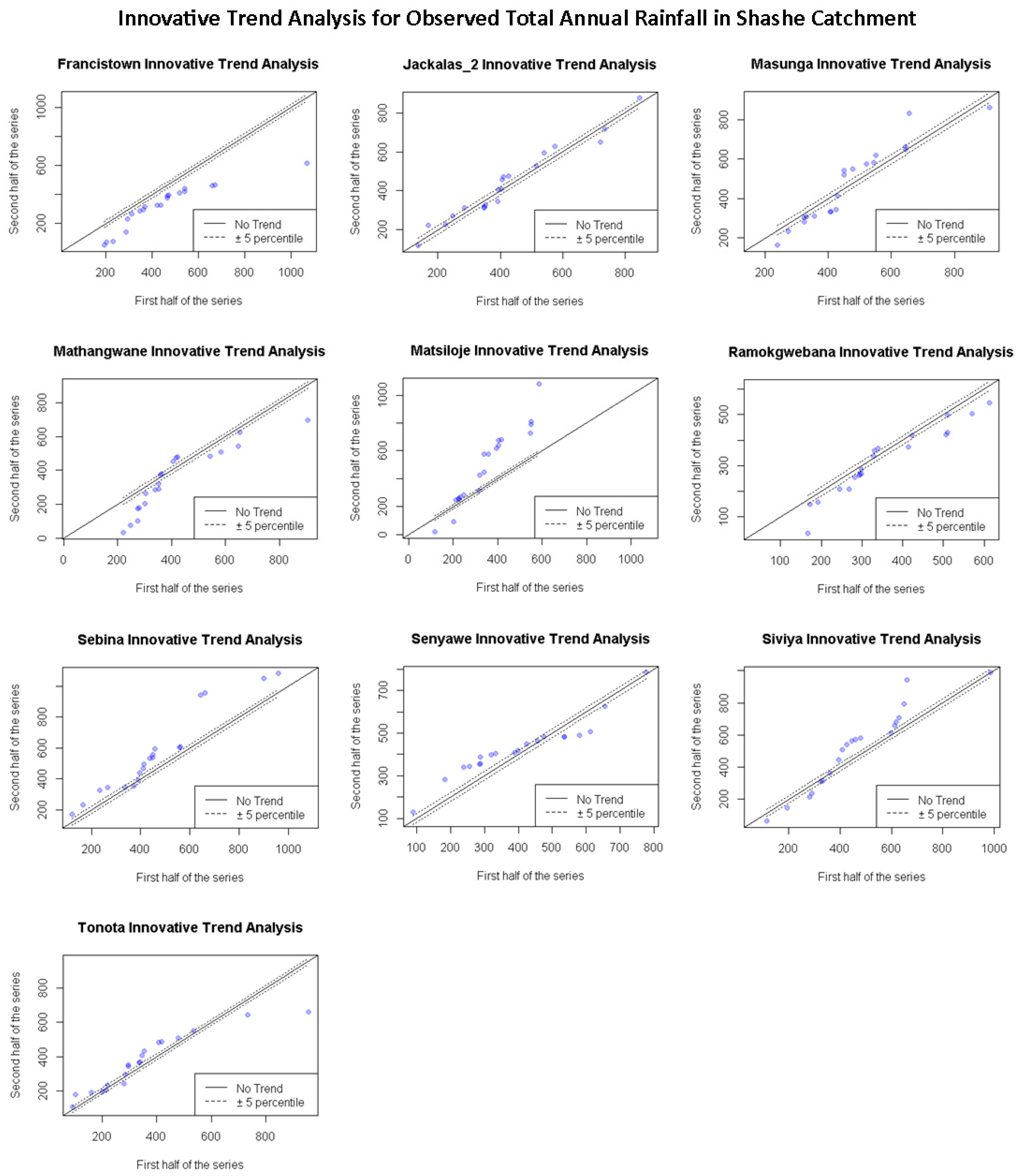
The trend results for the ITA method was plotted to visualize the pattern of rainfall for both observed and projected annual totals and annual maximums. According to ITA for observed total annual rainfall in Figure 8, there is decreasing trend in minimum values for Francistown, Masunga, Mathangwane, Matsiloje, Ramokgwebana, and Siviya. Conversely, an increase in trends for minimum values is observed in Tonota and Senyawe. Jackalas_2 shows no significant observable trend. An increase in the trend for maximum values is observed in Masunga, Matsiloje, Sebina and Siviya. In contrast, a decrease in the trend for maximum values for observed total rainfall is observed in Francistown, Mathangwane, Ramokgwebana, and Tonota.

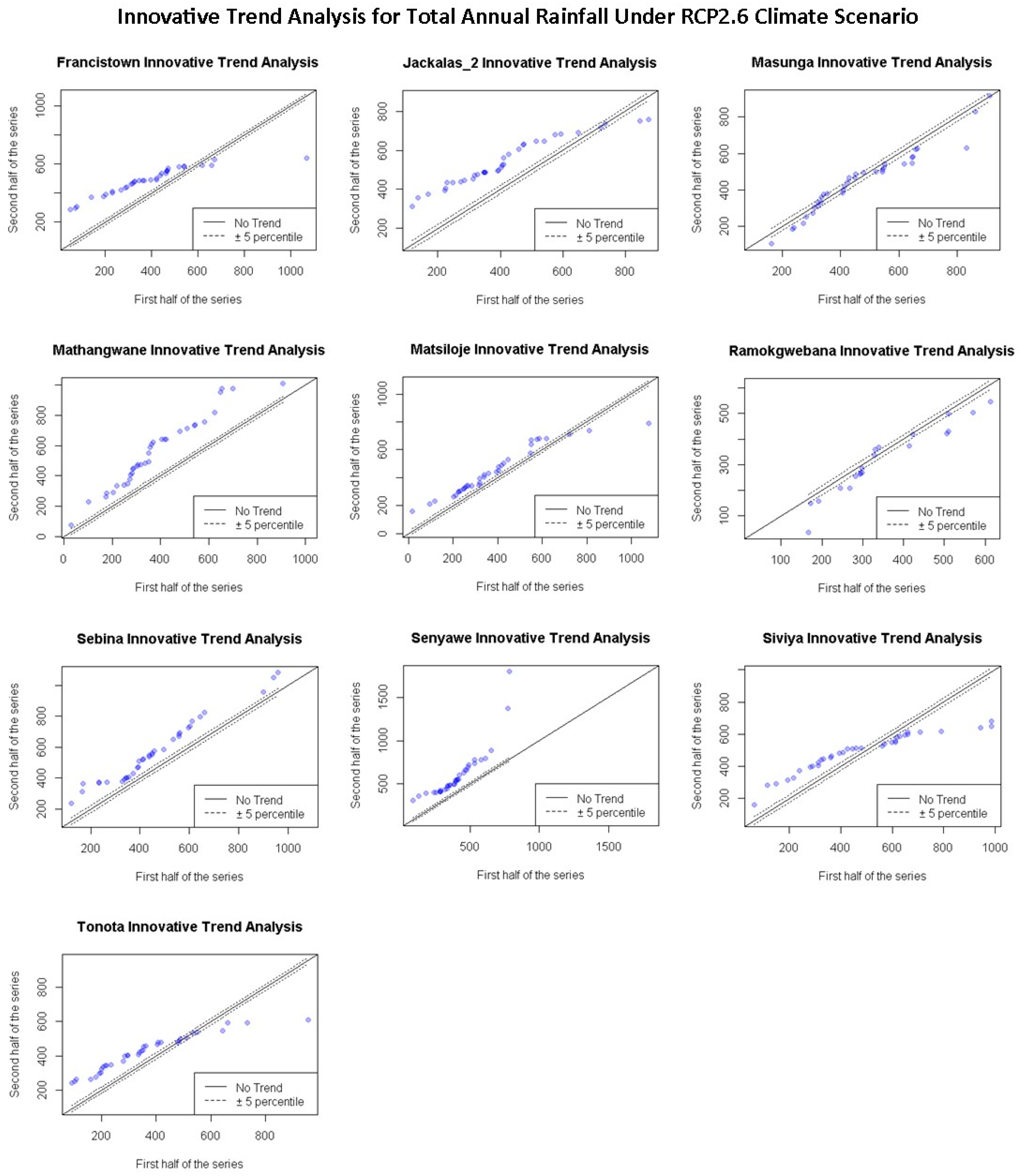
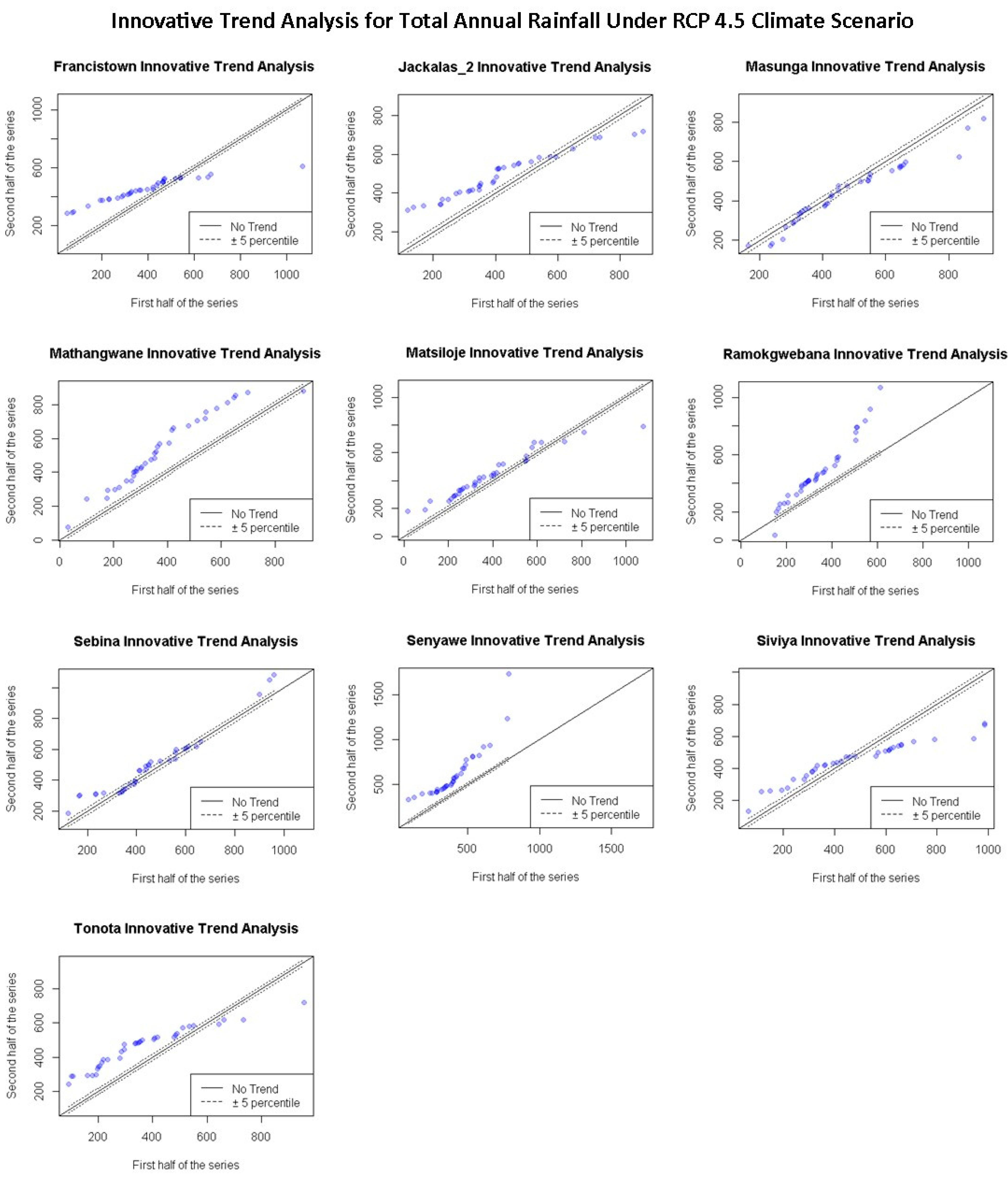
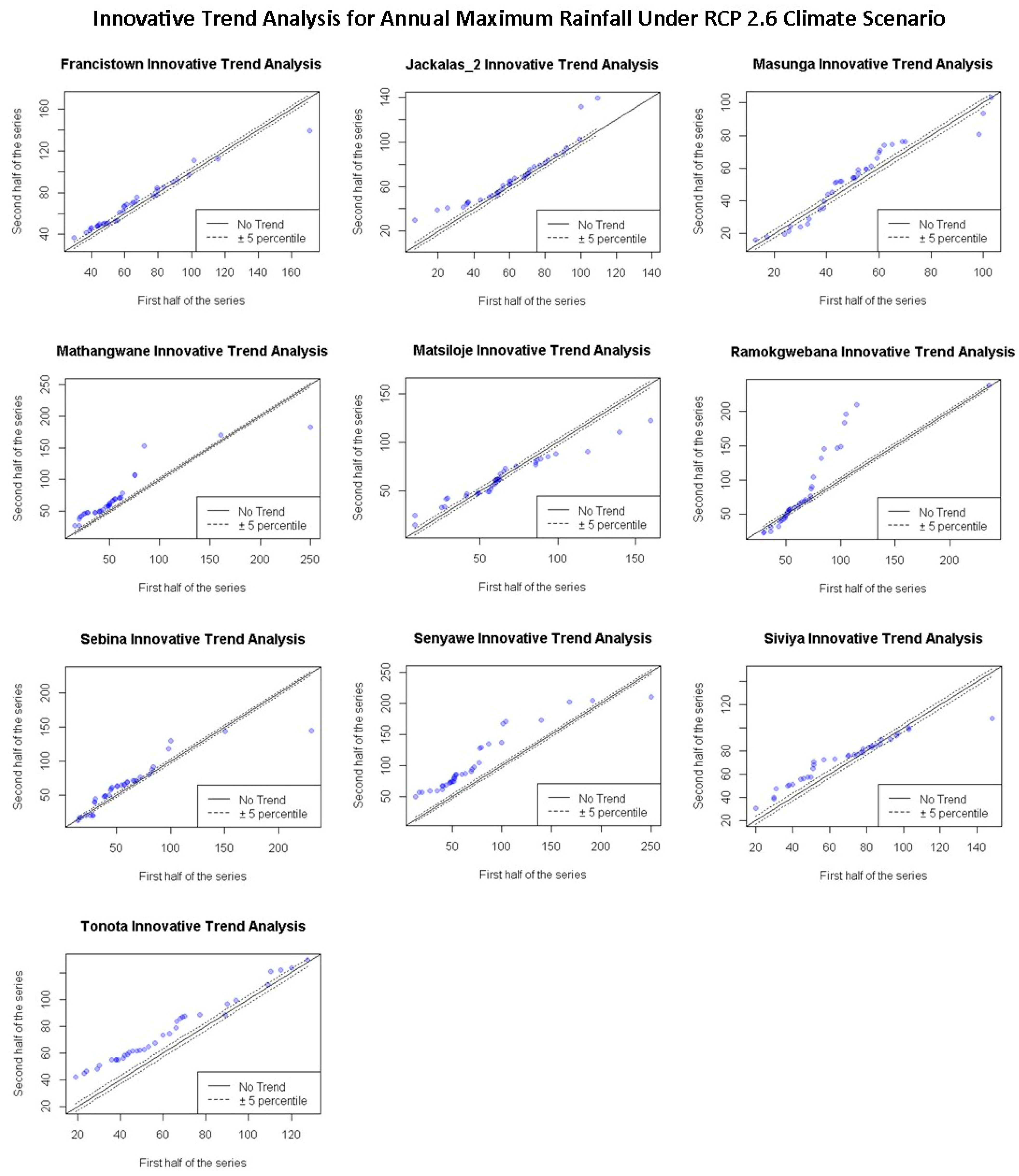
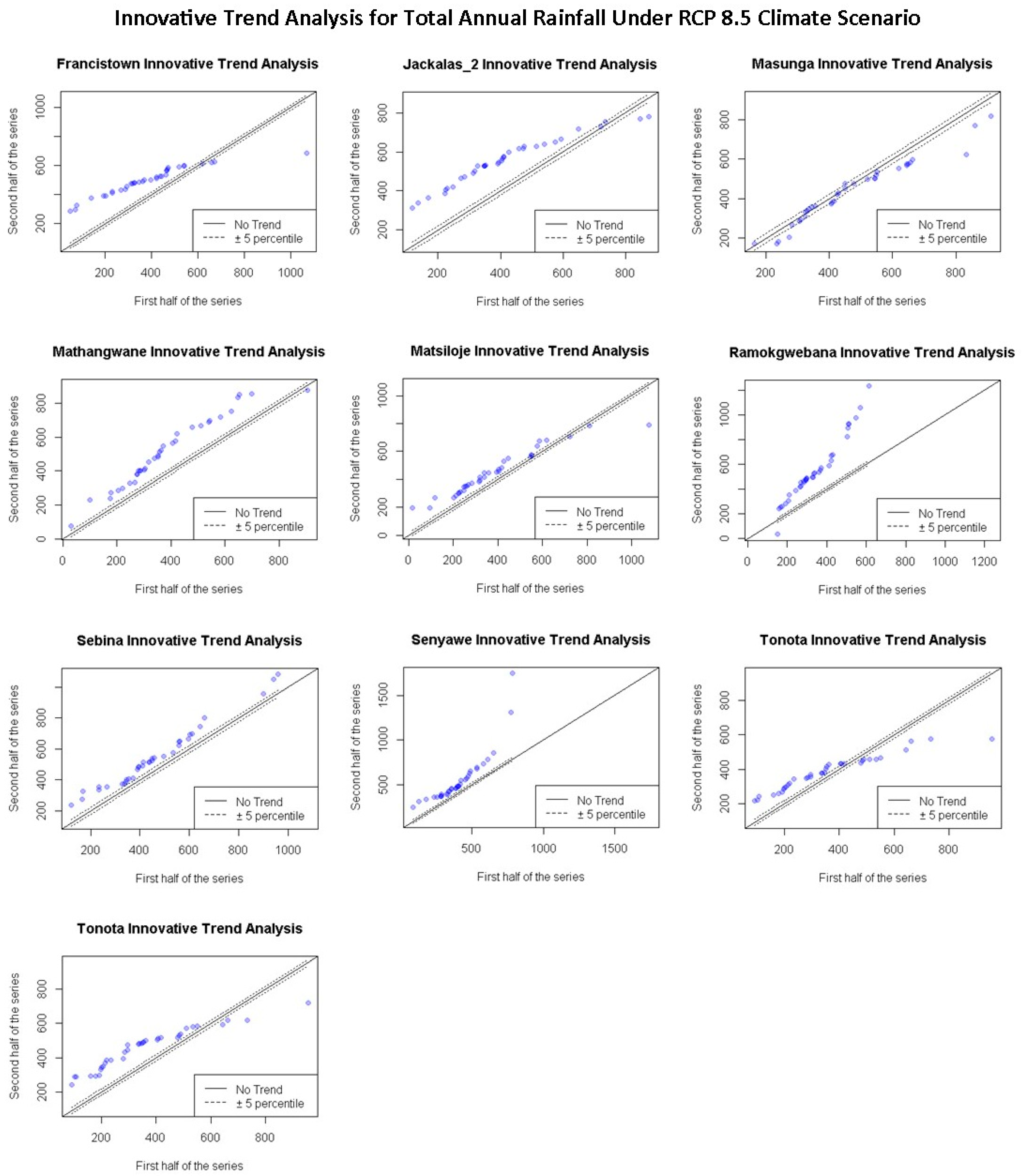
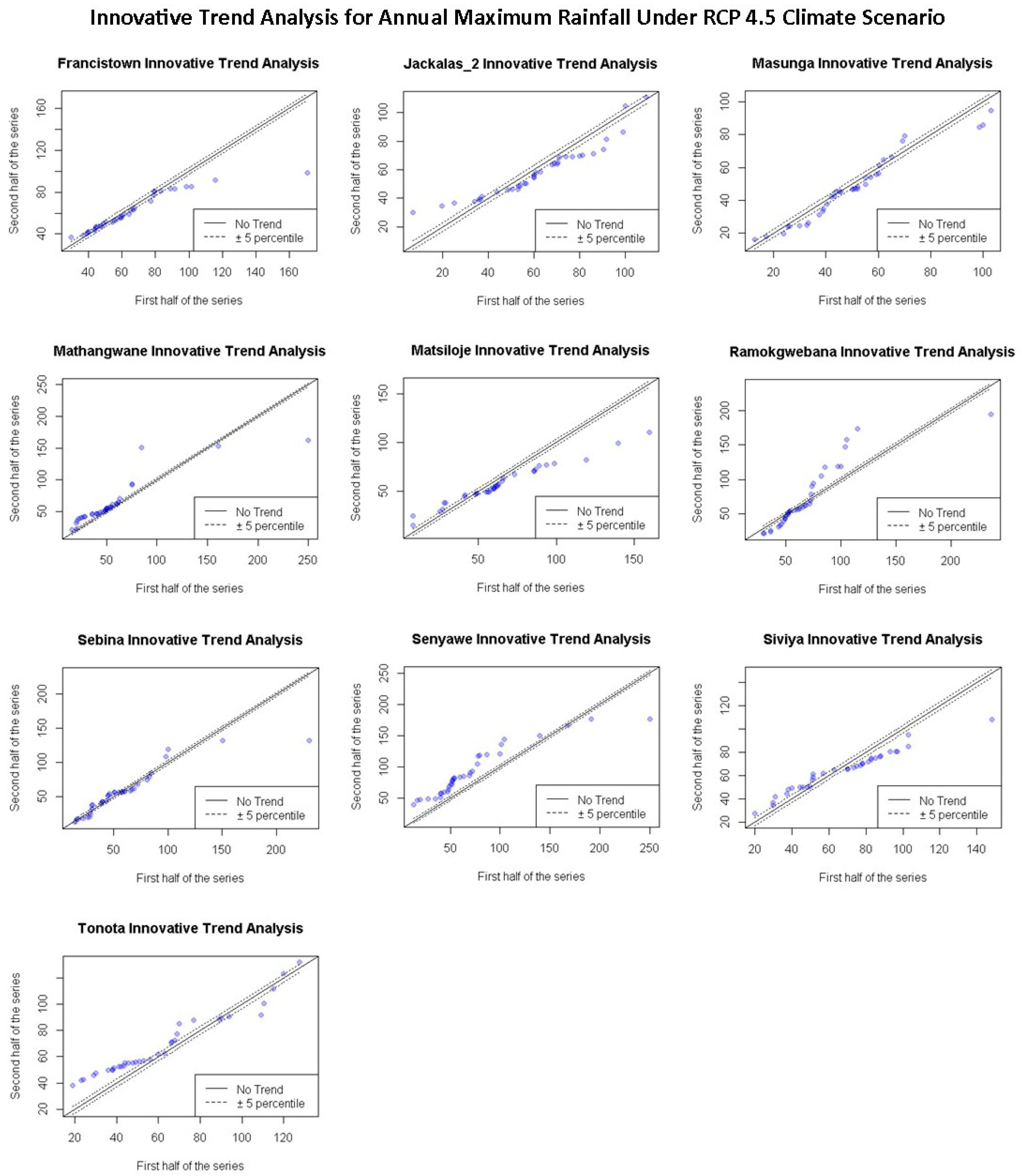
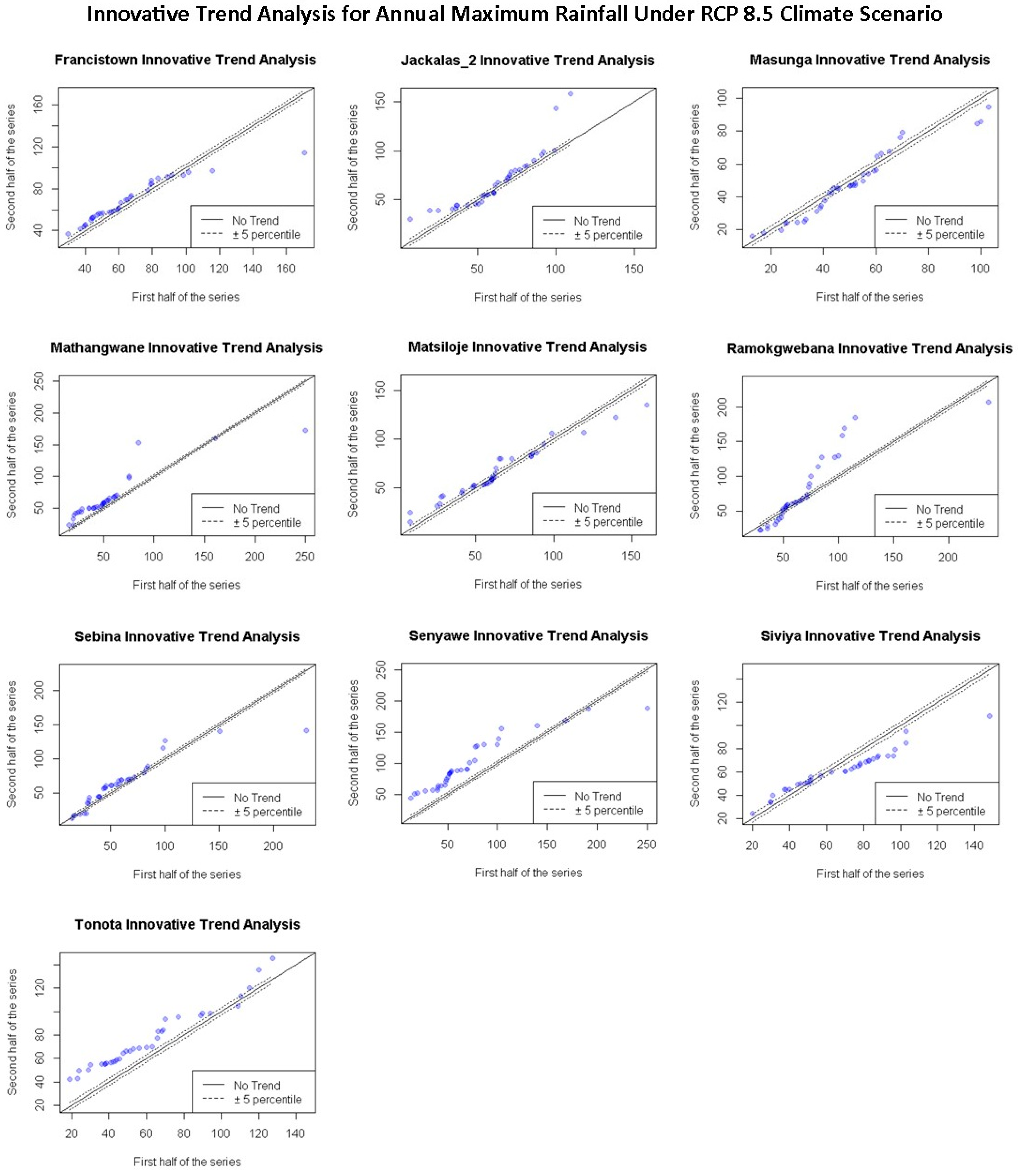
Trends for rainfall projections under RCP 2.6 scenario in Figure 9 shows an increasing trend in minimum values and a decrease in trends for maximum values, except for Mathangwane, Sebina and Senyawe, which show an increasing trend in maximum values. The same pattern is repeated for projected total annual rainfall under RCP 4.5 and 8.5 climate scenarios, as shown in Figure 10 and Figure 11. However, Ramokgwebana shows an increasing trend for minimum and maximum values under the RCP 8.5 climate scenario.

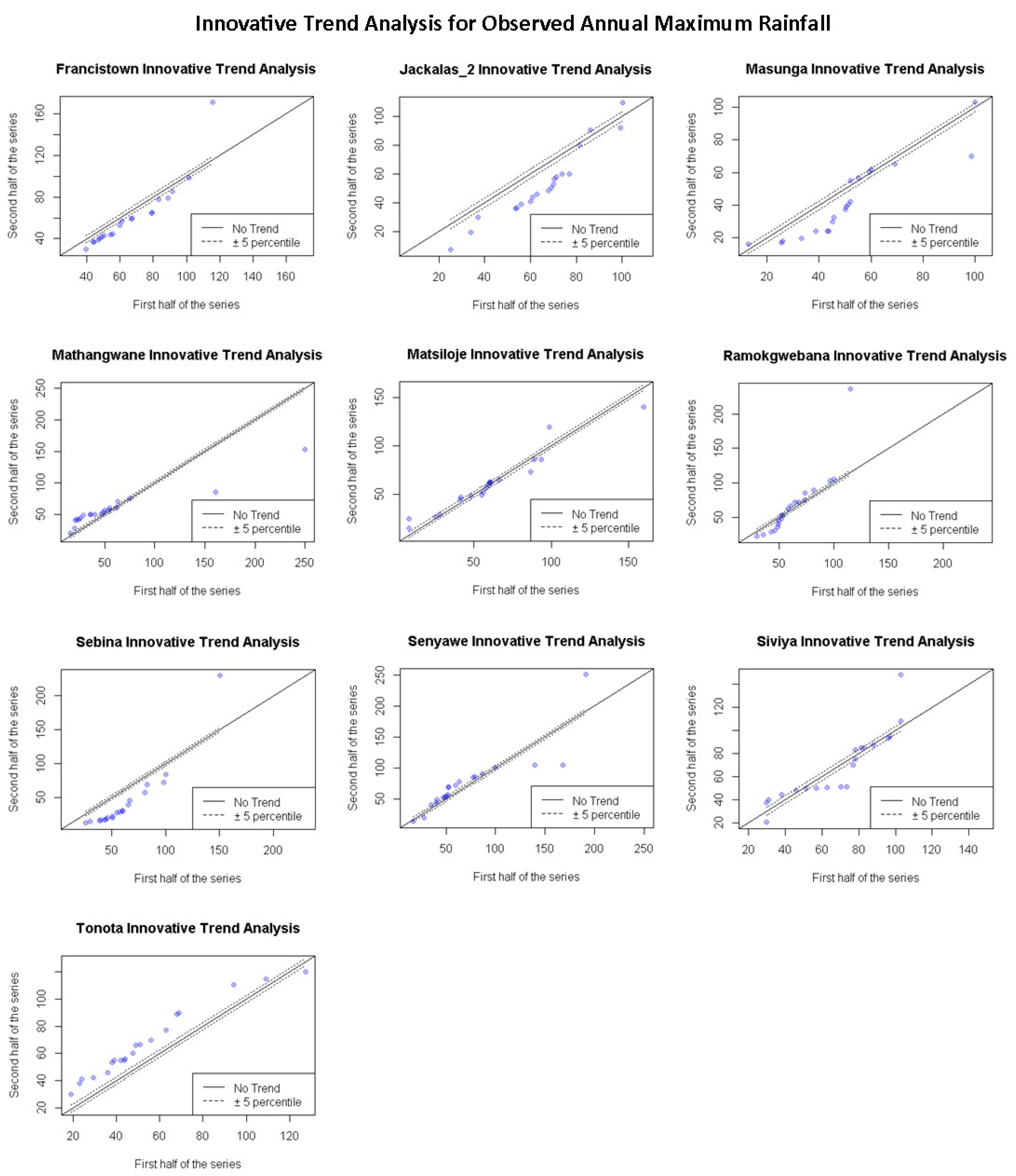
3.5. Mann-Kendall, Sen’s Slope and the Innovative Trends Analysis of Annual Maximum Rainfall for the Shashe Catchment

The Tau, Z-value and Sen’s Slope for observed annual maximum rainfall indicates a decreasing trend for Francistown, Jackalas_2, Masunga, Matsiloje, Ramokgwebana and Sebina by a range between 0–1 mm per year. The remaining four (Mathangwane, Senyawe, Siviya and Tonota) stations show an increase by a range between 0.3–0.9 mm per year, as shown in

Table 4. The trend for annual maximum rainfall and magnitude of trend between 1981–2020 for gauging stations in the study area.

		Location	Francistown	Jackalas_2	Masunga	Mathangwane	Matsiloje	Ramokgwebana	Sebina	Senyawe	Siviya	Tonota
MK	Tau	Observed	−0.148	−0.189	−0.213	0.347	−0.0064	−0.0488	−0.353	0.158	0.0758	0.165
		RCP 2.6	0.0840	0.1290	0.0680	0.2560	0.0740	0.1120	0.0980	0.2950	0.0350	0.2810
		RCP 4.5	−0.0120	0.0200	−0.0180	0.1670	−0.0090	0.0700	0.0320	0.2150	−0.1080	0.1950
		RCP 8.5	0.1180	0.0990	−0.0180	0.2250	0.0790	0.1150	0.0970	0.2780	−0.1310	0.2860
	p-Value	Observed	0.1841	0.0889	0.05448	0.00172	0.9628	0.6664	0.00141	0.1552	0.4991	0.1388
		RCP 2.6	0.3080	0.1150	0.4120	0.0020	0.3700	0.1710	0.2340	0.0000	0.6700	0.0010
		RCP 4.5	0.8830	0.8120	0.8310	0.0420	0.9150	0.3940	0.6960	0.0090	0.1890	0.0170
		RCP 8.5	0.1480	0.2260	0.8310	0.0060	0.3380	0.1620	0.2380	0.0010	0.1100	0.0000
	Z-Value	Observed	−1.3283	−1.7015	−1.9230	3.1351	−0.0466	−0.4312	−3.1926	1.4215	0.6759	1.4804
		RCP 2.6	1.0190	1.5770	0.8210	3.1230	0.8970	1.3690	1.1910	3.6050	0.4260	3.4270
		RCP 4.5	−0.1470	0.2380	−0.2130	2.0380	−0.1060	0.8520	0.3900	2.6310	−1.3130	2.3830
		RCP 8.5	1.4450	1.2120	−0.2130	2.7480	0.9580	1.3990	1.4450	3.4020	−1.5970	3.4980
Sen’s slope (mm)		Observed	−0.3082	−0.5848	−0.6093	0.9264	−0.0033	−0.1708	−0.9999	0.5929	0.3097	0.4771
		RCP 2.6	0.1300	0.2300	0.1100	0.4200	0.1100	0.2300	0.2100	0.7000	0.0500	0.5100
		RCP 4.5	−0.0100	0.0200	−0.0200	0.2300	−0.0100	0.1300	0.0500	0.5000	−0.1500	0.3100
		RCP 8.5	0.1800	0.1800	−0.0200	0.3600	0.1500	0.2400	0.2000	0.6600	−0.1900	0.5000
ITA	Trend Slope	Observed	−0.2528	−0.6325	−0.4372	−0.0059	0.0217	0.2370	−0.9505	0.1585	−0.0055	0.6580
		RCP 2.6	0.0734	0.1744	0.0657	0.3644	−0.0617	0.4134	0.1150	0.8456	0.1357	0.3832
		RCP 4.5	−0.1306	−0.0803	−0.0741	0.1639	−0.2092	0.1024	−0.0774	0.5350	−0.0994	0.1963
		RCP 8.5	0.0596	−0.0684	0.1798	0.2808	0.0416	0.2476	0.0895	0.7160	−0.1884	0.4177
	Trend Indicator	Observed	−0.7626	−1.9312	−1.7288	−0.0207	0.0722	0.7566	−3.0449	0.4434	−0.0160	2.4564
		RCP 2.6	0.3926	0.9922	0.4610	2.3519	−0.3388	2.1159	0.6937	4.1425	0.7045	2.1903
		RCP 4.5	−0.6987	−0.4566	−0.5199	1.0582	−1.1483	0.5243	−0.4664	2.6210	−0.5164	1.1219
		RCP 8.5	0.3187	−0.4798	1.0228	1.8127	0.2286	1.2675	0.5397	3.5077	−0.9781	2.3872

. Projected annual maximum rainfall shows contrary, positive trend results compared to negative observed rainfall values for Jackalas_2, Ramokgwebana and Sebina for all climate scenarios. In contrast, Francistown and Matsiloje show an increasing trend for RCP 2.6 and RCP 8.5 climate scenarios, while Siviya shows a decreasing trend for RCP 4.5 and 8.5 climate scenarios. It must be noted that the magnitude of Sen’s Slope trend ranges between −1 and 1 mm. The ITA method shows consistency in the direction of observed and projected trends for Ramokgwebana, Senyawe and Tonota for all climate scenarios. The same consistency is maintained for Francistown (RCP 4.5), Jackalas_2 (RCP 4.5 and 8.5, Masunga (RCP 4.5), Sebina (RCP 4.5) and Siviya (RCP 4.5 and 8.5). Inconsistencies between observed and projected annual maximum values are shown in Mathangwane for all climate scenarios, while Francistown, Jackalas_2, Masunga, Sebina, and Siviya for RCP 2.6. Inconsistencies are also notable between the trend magnitude of both Sen’s Slope and ITA.

The trend distribution for the ITA was also plotted for annual maximum rainfall for both observed and projected climate scenarios, as shown in Figure 12, Figure 13, Figure 14 and Figure 15. The plots for observed data sets show a decreasing trend for minimum values for Francistown, Jackalas_2, Masunga, Ramokgwebana, and Sebina. Only Mathangwane and Tonota show an increasing trend for minimum values. Matsiloje shows no significant visual trend, while Senyawe shows no significant trend for minimum values. There is a significant increasing trend in maximum values for Francistown, Ramokgwebana, Sebina, Siviya and Senyawe, as shown in Figure 12.

Climate projections of annual maximum rainfall are somewhat more similar to the pattern of the ITA trend. Francistown, Masunga, Ramokgwebana, and Sebina show no significant trend in minimum rainfall values, while no significant trend is observed for maximum rainfall in Tonota. On the other hand, Ramokgwebana and Jackalas_2 show an increasing trend in maximum rainfall values. In contrast, a decreasing trend in maximum rainfall is observed for Francistown, Masunga, Mathangwane, Matsiloje, Sebina, Senyawe and Siviya.

3.6. Sample L-Moment Test Statistics for Sites in the Region

Annual maximum rainfall was used to determine sample test statistics for each site in the study region, as shown in

Table 5. Sample L-moment test statistics for sites in the region for the 1981–2020 period.

Gauging Station	Record Length	Annual Maximum (mm)	L-CV (t)	L-Skewness (t3)	L-Kurtosis (t4)	Discordancy Measure (DI)
Francistown	40	63.76	0.2171	0.2868	0.1748	1.84
Jackalas_2	40	59.18	0.2223	0.0259	0.1368	1.11
Masunga	40	46.20	0.2654	0.1306	0.1464	0.29
Mathangwane	40	56.73	0.3274	0.3982	0.397	1.64
Matsiloje	40	60.38	0.286	0.1522	0.2502	0.9
Ramokgwebana	40	65.02	0.2649	0.2832	0.2607	0.41
Sebina	40	52.93	0.3713	0.3264	0.2405	2.2
Senyawe	40	73.08	0.3189	0.3163	0.2787	0.3
Siviya	40	68.69	0.2222	0.0412	0.0755	0.84
Tonota	40	60.16	0.2552	0.2146	0.1493	0.46

for observed data,

Table 6. Sample L-moment test statistics for sites in the region under RCP 2.6 climate scenario.

Gauging Station	Record Length	Annual Maximum	L-CV (t)	L-Skewness (t3)	L-Kurtosis (t4)	Discordancy Measure (DI)
Francistown	70	66.72	0.2007	0.2479	0.1501	1.95
Jackalas_2	70	64.57	0.2035	0.0832	0.1823	0.66
Masunga	70	50.14	0.2463	0.0648	0.1471	0.58
Mathangwane	70	60.60	0.2944	0.3653	0.3646	1.85
Matsiloje	70	62.67	0.2388	0.1245	0.2312	0.66
Ramokgwebana	70	75.61	0.3101	0.3742	0.2655	0.78
Sebina	70	60.06	0.319	0.2254	0.2208	1.15
Senyawe	70	86.24	0.3017	0.2901	0.2111	0.62
Siviya	70	69.78	0.1888	−0.0279	0.0942	0.99
Tonota	70	67.94	0.2309	0.1472	0.1049	0.75

under RCP 2.6,

Table 7. Sample L-moment test statistics for sites in the region under RCP 4.5 climate scenario.

Gauging Station	Record Length	Annual Maximum	L-CV (t)	L-Skewness (t3)	L-Kurtosis (t4)	Discordancy Measure (DI)
Francistown	70	63.15	0.1894	0.2351	0.1351	1.96
Jackalas_2	70	60.12	0.1965	0.0597	0.1533	0.69
Masunga	70	47.81	0.2464	0.1085	0.1727	0.5
Mathangwane	70	57.10	0.2921	0.3719	0.3803	2.14
Matsiloje	70	60.09	0.2369	0.1448	0.2591	0.89
Ramokgwebana	70	70.17	0.2875	0.3246	0.2441	0.51
Sebina	70	56.69	0.3177	0.2566	0.2443	1.13
Senyawe	70	80.81	0.2936	0.2726	0.1903	0.85
Siviya	70	65.67	0.1931	0.0373	0.1214	0.79
Tonota	70	64.67	0.2303	0.1898	0.1275	0.53

under RCP 4.5, and

Table 8. Sample L-moment test statistics for sites in the region under RCP 8.5 climate scenario.

Gauging Station	Record Length	Annual Maximum	L-CV (t)	L-Skewness (t3)	L-Kurtosis (t4)	Discordancy Measure (DI)
Francistown	70	66.48	0.1888	0.2068	0.1385	1.84
Jackalas_2	70	64.67	0.2172	0.1221	0.175	0.4
Masunga	70	47.81	0.2464	0.1085	0.1727	0.58
Mathangwane	70	59.14	0.2908	0.3589	0.3762	2.34
Matsiloje	70	64.48	0.2479	0.1406	0.2218	0.66
Ramokgwebana	70	72.71	0.2909	0.3306	0.2545	0.81
Sebina	70	59.61	0.3159	0.2307	0.2261	1.16
Senyawe	70	83.97	0.293	0.2579	0.1844	0.98
Siviya	70	64.11	0.1982	0.0767	0.1297	0.72
Tonota	70	68.54	0.2333	0.1584	0.1237	0.5

under RCP 8.5 climate scenario. These test statistics are based on their position in the L-loment ratio diagram. The L-moment ratio diagram is developed based on the scatter plot of L-skewness (t3) and L-kurtosis (t4) for the ten sites of the study region concerning different 3-parameter distributions. This is used to choose a distribution that best fits the data.

The goodness of fit of a distribution is determined by how well L-skewness and L-kurtosis of the fitted distribution match the regional weighted means of L-skewness and L-kurtosis of the observed data [81]. The regional average L-skewness and L-kurtosis are shown in

Table 9. The regional average L-moment ratios for records between 1981–2020 and under RCP 2.6, 4.5 and RCP 8.5 climate scenarios.

	L-CV (t)	L-Skewness (t3)	L-Kurtosis (t4)
1981–2000	0.2751	0.2175	0.211
RCP 2.6	0.2534	0.1895	0.1972
RCP 4.5	0.2483	0.2001	0.2028
RCP 8.5	0.2523	0.1991	0.2003

. Notably, the discordancy measure of all the sites in all four different study periods is less than the 2.491 critical value. This indicates that the study region is homogeneous.

3.7. Heterogeneity Measure for the Region

The heterogeneity (H) measure for the region based on L-skew/L-kurtosis ratios was determined for all the study periods based on 500 simulations, as indicated in

Table 10. Heterogeneity measure for the region for records between 1981–2020 and under RCP 2.6, 4.5 and RCP 8.5 climate scenarios.

	1981–2020	RCP 2.6	RCP 4.5	RCP 8.5
Observed s.d. of L-skew/L-kurtosis distance	0.1327	0.1316	0.118	0.101
Sim. mean of s.d. of L-skew/L-kurtosis distance	0.1046	0.0768	0.0781	0.079
Sim. s.d. of s.d. of L-skew/L-kurtosis distance	0.0244	0.0165	0.0179	0.0174
Heterogeneity measure H [3]	1.15	3.31	2.23	1.26

Note: s.d. devotes standard deviation, Sim. denotes simulated.

below. The results show that the heterogeneity measure based on the L-skew/L-kurtosis ratio is the perfect fit for the study area since all the H values are less than the threshold for heterogeneity. A region is considered heterogeneous if H is sufficiently large. When H ≥ 2, the region is homogeneous if H < 1 and possibly homogeneous if 1 ≤ H < 2. Data for 1981–2020, the period under RCP 8.5 is acceptably homogeneous as H is between 1 ≤ H < 2; under RCP 2.6 and RCP4.5, the region is considered heterogeneous as H ≥ 2.

3.8. Goodness-of-Fit Statistical Measure and Parameter Estimates for Distributions

For this study five distributions with three parameters Generalized Logistic (GLO), Generalized Extreme Value (GEV), Generalized Pareto (GPA), Log-Normal (LNO), and Pearson type III (PIII) are fitted regional average L-moment ratios. The Z^DIST goodness-of-fit measure selects a distribution that gives the closest estimate as observed data. A region is considered homogeneous if $Z^{DIST}$ if it is close to zero and it is acceptable of $\left|Z^{DIST}\right|\le 1.64$. The results in

Table 11. The Z-Value Goodness-of-Fit statistical measure.

Probability Distributions	1981–2020	RCP 2.6	RCP 4.5	RCP 8.5
Gen. logistic	−0.64 *	−0.26 *	−0.48 *	−0.23 *
Gen. extreme value	−1.94	−2.23	−2.36	−2.09
Gen. normal	−2.35	−2.62	−2.8	−2.53
Pearson type III	−3.14	−3.47	−3.73	−3.43
Gen. Pareto	−5.05	−6.73	−6.72	−6.4

* Indicates best fit distribution.

indicate that Generalized logistics is the only best-fit distribution for observed and under-climate projections. All other distributions have a Z-Value greater than 1.64; hence not fit for further analysis. Parameters estimates for the best fit Generalized Logistic distribution were determined as indicated in

Table 12. Parameter estimates for Generalised Logistic distribution accepted at 0.90 confidence level.

	L-CV (t)	L-Skewness (t3)	L-Kurtosis (t4)
1981–2020	0.9038	0.2542	−0.2175
RCP 2.6	0.9224	0.2387	−0.1895
RCP 4.5	0.9199	0.2323	−0.2001
RCP 8.5	0.919	0.2361	−0.1991

.

3.9. Estimation of the Quantiles

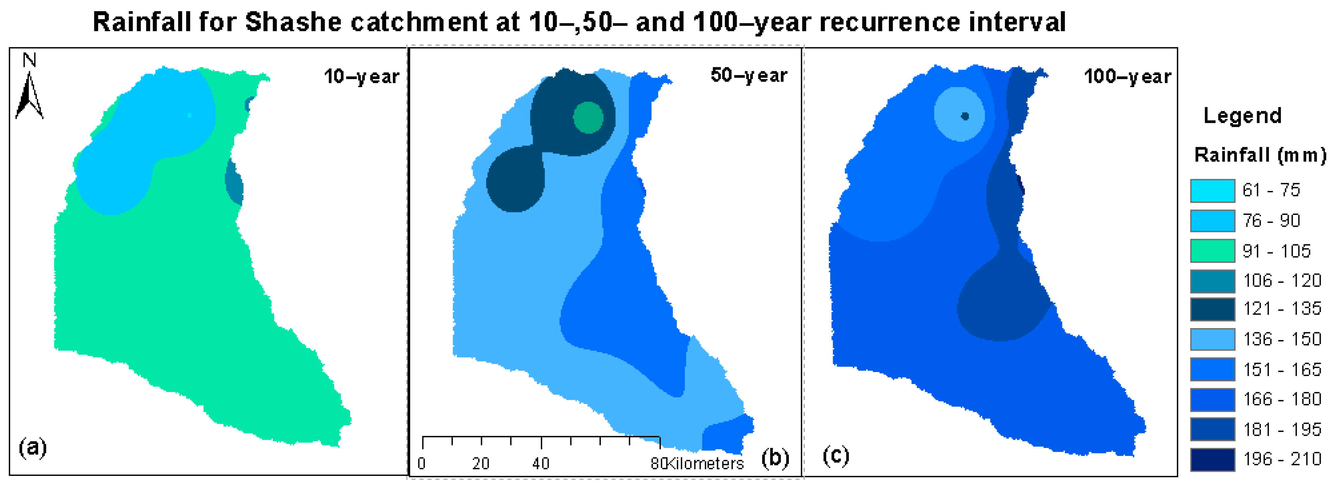
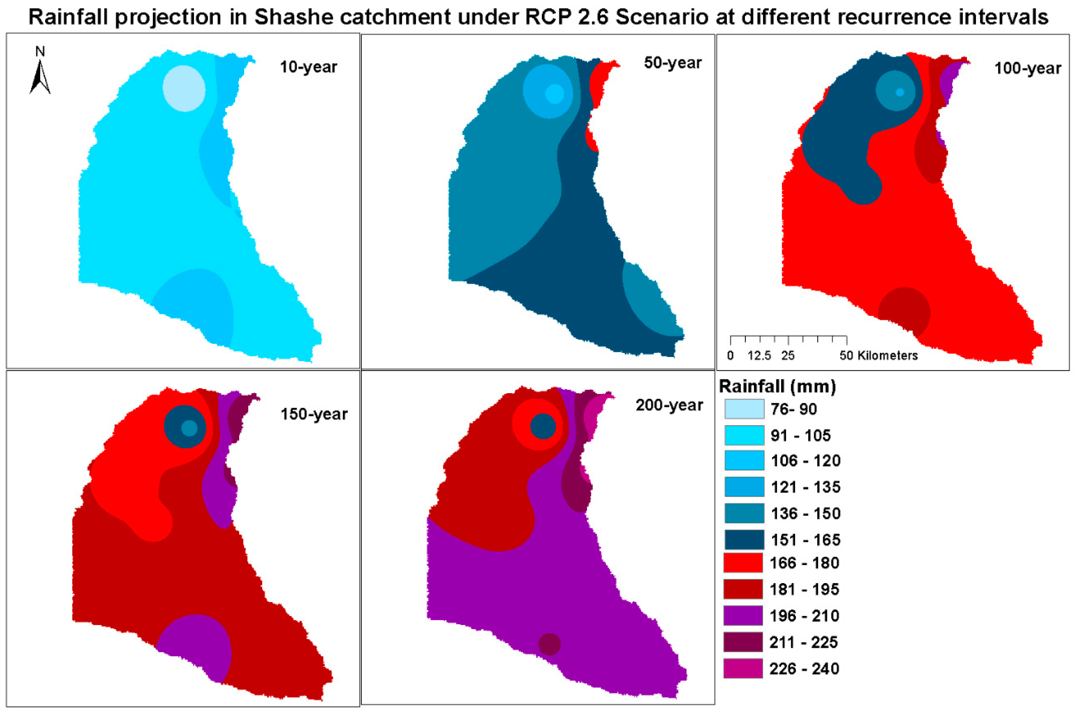
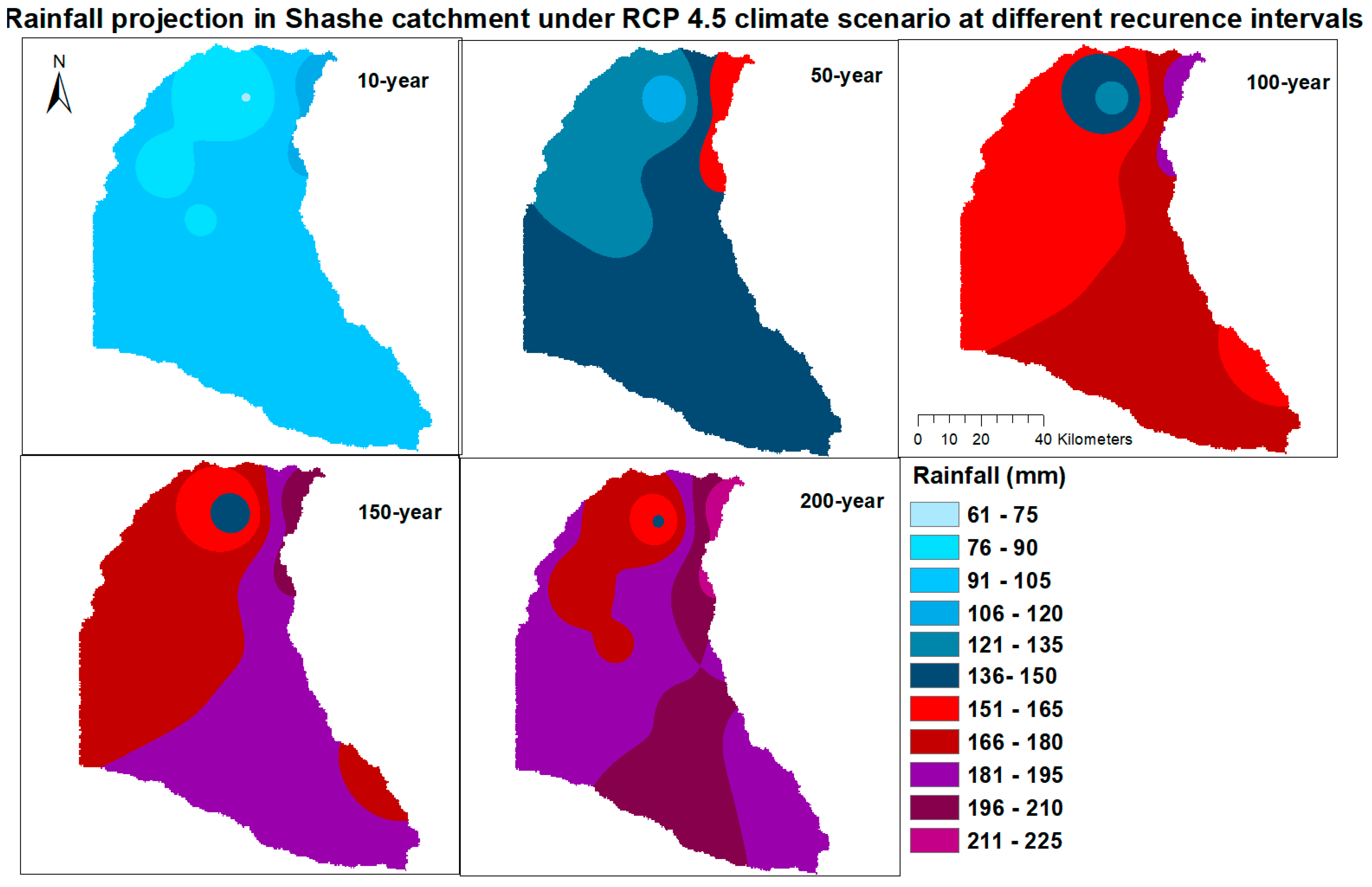
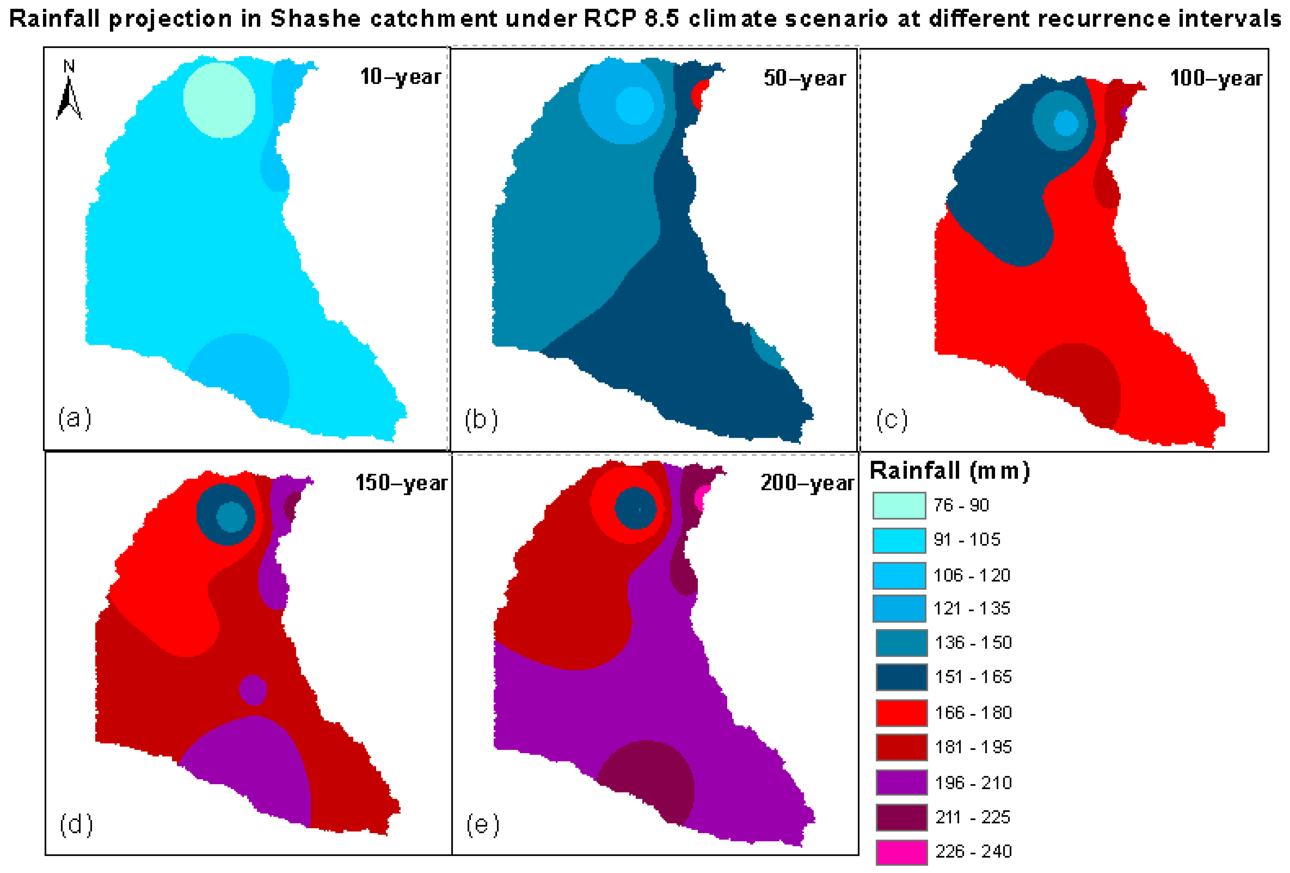
Parameter estimates for Generalised Logistic distributions were used for the estimation of quantiles. Three recurrence intervals (10-year, 50-year, and 100-year) were estimated using observed data with associated quantiles. First, quantiles for each rainfall gauging station were estimated, and the spatial distribution of each quantile was mapped in the study using the distance inverse Interpolation method, as shown in Figure 16. Then, the same approach was repeated using climate projections. However, the quantiles were estimated for 10-year, 50-year, 100-year, 150-year and 200-year recurrence intervals, as shown in Figure 17, Figure 18 and Figure 19. Corresponding areal coverage for spatial rainfall distribution for each recurrence interval was also computed. Changes in areal coverage are indicated in

Table 13. Areal change in rainfall distribution at 10–year, 50–year and 100–year recurrence intervals in the study area for the 1981–2020 study period.

Rainfall (mm)	10–Year Area (km2)		50–Year Area (km2)		100–Year Area (km2)
61–75	11
76–90	1434	(99%)
91–105	6095
106–120	76		87
121–135			960		5
136–150			4468	(86%)	231
151–165			2095		1584	(81%)
166–180			6		4661
181–195					1128
196–210					7

Note: The percentage in brackets represents the rainfall range with the largest spatial coverage.

,

Table 14. Areal change in rainfall distribution under RCP 2.6 climate scenario at 10–year, 50–year, 100–year, 150–year and 200–year recurrence intervals.

Rainfall (mm)	10–Year Area (km2)		50–Year Area (km2)		100–Year Area (km2)		150–Year Area (km2)		200–Year Area (km2)
76–90	271
91–105	6013	(96%)
106–120	1334		55
121–135			346		9
136–150			3663	(92%)	199		34
151–165			3396		1504	(87%)	205		87
166–180			156		5120		1537	(82%)	252
181–195					688		4764		1996	(89%)
196–210					96		933		4776
211–225							143		389
226–240									116

Note: The percentage in brackets represents the rainfall range with the largest spatial coverage.

,

Table 15. Areal change in rainfall distribution under RCP 4.5 climate scenario at 10–year, 50–year, 100–year, 150–year and 200–year recurrence intervals.

Rainfall (mm)	10–Year Area (km2)		50–Year Area (km2)		100–Year Area (km2)		150–Year Area (km2)		200–Year Area (km2)
76–90	6
91–105	1162	(97%)
106–120	6293
121–135	155		167
136–150			1985	(94%)	84
151–165			5190		392		120		12
166–180			274		3494	(92%)	422		190
181–195					3500		3376	(91%)	1246
196–210					146		3517		3913	(79%)
211–225							181		2121
226–240									134

Note: The percentage in brackets represents the rainfall range with the largest spatial coverage.

and

Table 16. Areal change in rainfall distribution under RCP 8.5 climate scenario at 10–year, 50–year, 100–year, 150–year and 200–year recurrence intervals.

Rainfall (mm)	10–Year Area (km2)		50–Year Area (km2)		100–Year Area (km2)		150–Year Area (km2)		200–Year Area (km2)
76–90	466
91–105	6231	(94%)
106–120	919
121–135			123
136–150			501		59
151–165			3438	(91%)	255		87
166–180			3520		1819	(83%)	259		146
181–195			34		4524		1755		331
196–210					951		4034	(92%)	2110	(82%)
211–225					8		1442		4173
226–240							39		820

Note: The percentage in brackets represents the rainfall range with the largest spatial coverage.

.

Generally, it can be observed that 10-year rainfall quantiles have less variability in spatial coverage compared to other return intervals. In a 10-year return interval for observed data, RCP 2.5 and RCP 8.5, a rainfall range between 91–120 mm covers at least 94% area of the entire catchment. Similarly, a 10-year rainfall range between 106–120 under RCP 4.5 covers over 80% of the entire catchment area. It is also observed that under climate projections, spatial areal coverage for lower rainfall ranges decreases while higher rainfall ranges increase. For example, a 50-year rainfall with magnitude 136–165 mm will have spatial areal coverage around 86%, 92% and 94% based on observed RCP 2.6 and RCP 4.5, respectively, when it happens. Spatial coverage of a 100-year rainfall between 151–180 will be 81% based on observed data and 87% based on projected data under RCP 2.6 scenario. Under RCP 4.5 scenario, 92% of the area will be covered by rainfall between 166–195 mm. A 150-year rainfall with high spatial coverage will be of magnitude 166–195 mm (82%) under RCP 2.6 scenario, 181–210 mm (91%) under RCP 4.5 scenario and 181–210 mm (91%) under RCP 8.5 scenario. A 200-year rainfall that ranges between 196–225 mm under RCP 4.5 and 8.5 have high spatial coverage of at least 79% and 82%, respectively.

4. Discussion

Climate change has brought uncertainties and variations in hydro-metrological events by increasing and decreasing temperature trends, rainfall, droughts, and floods. Therefore, necessary to improve scientific research on hydro-climatic variables to reduce associated risks. This study analyses the characteristics of annual total and annual maximum rainfall for observed and under-projected climate scenarios. Annual total rainfall characteristics are required for water resources planning and management, while annual maximum rainfall characteristics are necessary for disaster management and risk assessment.

The Long Ashton Research Station Weather Generator (LARS-WG) statistical downscaling model was applied to downscale rainfall data from ten gauging stations in the Shashe catchment. Its performance was assessed using the Chi-square, t-test, and f-test statistics alongside their p-values at a 5% significance level. Generally, the Chi-square and t-test performed well, with over 95% of datasets having a p-value greater than the 0.05 critical value details in Appendix B section Table A2. Three distinctive trend analysis methods and one frequency analysis method were used in this study. The Mann-Kendall method for trend detection, Sen’s Slope to determine the magnitude of the trend, and the Innovative Trends Analysis (ITA) for quantifying and visualizing the distribution of trends. Regional frequency analysis based on L-moment was applied to annual maximums of observed and future rainfall projections to determine the magnitude of rainfall at given recurrence intervals. The magnitudes of rainfall were then mapped to provide a visual representation of rainfall in various scenarios.

Table 3 shows that there are inconsistencies between observed and projected total annual rainfall for all trend detection methods. Francistown Mathangwane and Ramokgwebana show a decrease in observed rainfall while futuristic projections are increasing. Observed total rainfall trends for Masunga, Matsiloje, Sebina and Siviya are increasing while projections are decreasing for both Sen’s Slope and ITA method.

Analysis of total annual rainfall based on the ITA plot shows a decreasing trend in rainfall for minimum values for Francistown, Masunga, Mathangwane, Matsiloje, Ramokgwebana, and Siviya in Figure 8, Figure 9, Figure 10 and Figure 11. An increase in trends for minimum values is observed in Tonota and Senyawe. Jackalas_2 shows no significant observable trend. An increase in the trend for maximum values is observed in Masunga, Matsiloje, Sebina and Siviya. In contrast, a decrease in the trend for maximum values for observed total rainfall is observed in Francistown, Mathangwane, Ramokgwebana, and Tonota as shown in Figure 8. Trends for total rainfall projections under RCP 2.6 scenario in Figure 9 shows an increasing trend in minimum values and a decrease in trends for maximum values, except for Mathangwane, Sebina and Senyawe, which show an increasing trend in maximum values. The same pattern is repeated for projected total annual rainfall under RCP 4.5 and 8.5 climate scenarios, as shown in Figure 10 and Figure 11. However, Ramokgwebana shows an increasing trend for minimum and maximum values under the RCP 8.5 climate scenario.

As for annual maximum rainfall, the ITA method shows consistency in the direction of observed and projected trends for Ramokgwebana, Senyawe and Tonota for all climate scenarios. The same consistency is maintained for Francistown (RCP 4.5), Jackalas_2 (RCP 4.5 and 8.5, Masunga (RCP 4.5), Sebina (RCP 4.5) and Siviya (RCP 4.5 and 8.5). However, inconsistencies between observed and projected annual maximum values are shown in Mathangwane for all climate scenarios, while Francistown, Jackalas_2, Masunga, Sebina, and Siviya for RCP 2.6. Inconsistencies are also notable between the trend magnitude of both Sen’s Slope and ITA.

The trend distribution for the ITA for annual maximum rainfall for both observed and projected climate scenarios is shown in Figure 12, Figure 13, Figure 14 and Figure 15. The plots for observed data sets show a decreasing trend for minimum values for Francistown, Jackalas_2, Masunga, Ramokgwebana, and Sebina. Only Mathangwane and Tonota show an increasing trend for minimum values. There are notable high outlying points with maximum values for Francistown, Ramokgwebana, Sebina, Siviya, and Senyawe, have shown in Figure 12. Climate projections of annual maximum rainfall distribution pattern plots using ITA for Francistown, Masunga, Ramokgwebana, and Sebina show no significant trend in minimum rainfall values also, no significant trend is observed for maximum rainfall in Tonota. Ramokgwebana and Jackalas_2 show an increasing trend in maximum rainfall values, while decreasing trend in maximum rainfall is observed for Francistown, Masunga, Mathangwane, Matsiloje, Sebina, Senyawe and Siviya.

There is large rainfall variability in semi-arid regions, unlike in monsoon and tropical regions with less rainfall variability. Inconsistencies in trend analysis methods are prevalent in hydro-metrological studies. A recent study by [47,48] found inconsistencies between Mann–Kendall test, the Modified Mann–Kendall (MMK) and the innovative trend analysis (ITA) method when analyzing precipitation data. Rainfall trends have also been found by several studies to be more unstable compared to temperature. Discrepancies between observed and projected trends may be due to significant uncertainties in climate model simulations [3,82], and difficulties in climate models in understanding local climate processes [83]. A study by [84,85] also indicated that uncertainties in hydrological regimes might be due to climate scenarios, General Circulation Models (GCMs), and the choice of downscaling method.

The catchment is homogeneous as there is no discordant site in the region. The discordancy measure of all the sites in all four different study periods is less than the 2.491 critical value. Data for the 1981–2020 period and under RCP 8.5 is acceptably homogeneous as heterogeneity measure (H) is between 1 ≤ H < 2 while under RCP 2.6 and RCP4.5, the region is considered heterogeneous as H ≥ 2. Even though RCP 2.6 and RCP 4.5 were heterogeneous, they were also included in the analysis for comparison purposes. The Generalized Logistic distribution was the best-fit distribution for observed and under-climate projection data. The assessment was based on the Z-Value, which is less than the critical value of 1.64. Therefore, it was used to estimate the quantiles for the region.

The quantiles have been estimated using the Generalized Logistic distribution. For observed data, quantiles were estimated for the following recurrence intervals: 10-, 50-, 100-year, while for combined dataset (observed and projected climate scenarios), quantiles were estimated for 10-, 50-, 100-, 150-, 200-year. The selection of these frequencies is based on the fact that return intervals should not be more than three times the size of the datasets, beyond which the accuracy reduces [18]. It is also necessary to include higher recurrence intervals since previous extreme rainfall within and beyond 150 and 200-year quantiles has been recorded recently. Typically, between 1991–2011 over seven rainfall gauging stations recorded rainfall between 148–250 mm, consistent with 150 and 200-year recurrence intervals, with the highest being 250 mm recorded in Senyawe in 2004. It is observed in Table 14, Table 15 and Table 16 that under climate projections, spatial areal coverage for lower rainfall ranges decreases while higher rainfall ranges increase. In a 10-year return interval for RCP 8.5, a rainfall range between 91–120 mm covers at least 94% of the entire catchment area. Similarly, a 10-year rainfall range between 106–120 mm under RCP 4.5 covers over 80% of the entire catchment area. A 50-year rainfall with magnitude 136–165 mm will have spatial areal coverage around 86%, 92% and 94% based on observed RCP 2.6 and RCP 4.5, respectively, when it happens. Spatial coverage of a 100-year rainfall between 151–180 will be 81% based on observed data and 87% based on projected data under RCP 2.6 scenario. Under RCP 4.5 scenario, 92% of the area will be covered by rainfall between 166–195 mm. A 150-year rainfall with high spatial coverage will be of magnitude 166–195 mm (82%) under RCP 2.6 scenario, 181–210 mm (91%) under RCP 4.5 scenario and 181–210 mm (91%) under RCP 8.5 scenario. A projected 200-year rainfall that ranges between 196–225 mm under RCP 4.5 and 8.5 is likely to have a spatial coverage of at least 79% and 82%, respectively.

These results agree with a study by [15], which indicates that Botswana’s population exposed to floods is likely to increase by 100% if the temperature rises by 3 °C. For instance, a 100-year rainfall higher than 181 mm has a spatial coverage of only 15% under current conditions compared to over 95% coverage under RCP 8.5 future climate scenario.

It is also observed that under climate projections, spatial areal coverage for lower rainfall ranges decreases while higher rainfall ranges increase. The interpretation of the result is that if a rainfall of high magnitude is to happen, it is highly likely to have more spatial coverage. Another notable observation is that rainfall increases from the west and northwest towards the east and northeastern parts of the catchment. The west and northwest receive relatively lower rainfall than the east and northeastern parts of the catchment. The north and northeastern are currently receiving rainfall of high magnitudes, and projections indicate that the magnitudes will increase further. This combination will increase rainfall runoff downstream, increasing the likelihood of floods.

One interesting discovery in this study is that floods have been hitting most places in the catchment, such as Francistown, the second capital city, because of its location relative to rainfall spatial distribution. For example, Francistown is in the eastern part of the catchment, which receives high rainfall magnitude. It is also located at the confluence of two significant rivers whose upstream is developed and receives high rainfall. Even though extreme rainfall is decreasing in the Francistown area, as indicated in Table 3 and Table 4, other factors, such as high-intensity rainfall and a combination of changing land use which increases surface runoff and reduces infiltration, can influence floods. Land use change has the potential to shift the natural hydrological and hydro-ecological cycles and processes, resulting in changes in structures, forces and parameters driving these cycles [86,87,88]. It can modify the runoff process, increasing risk and vulnerability to climate change and associated natural disasters such as floods. Land use modification has a significant influence in determining time to concentration, travel time and discharge volume. Urban development lowers retardancy to flow, reduces infiltration rate, and decreases the time of concentration and travel time due to increasing the peak discharge [19,89,90,91,92,93]. Therefore, it is unsurprising that despite insignificant trends in extreme rainfall events, floods are experienced in the catchment. Therefore, this study recommends further studies on the potential effect of land use change on the rainfall-runoff process.

5. Conclusions

Efficient water resource management and flood risk management are necessary to ensure sustainable water resources and reduce vulnerability and exposure to infrastructure and people. Detection of trends and magnitude of floods at different return periods form the basis for water resource planning and management and flood risk assessment at both local and regional scales. This study presented a robust trend detection method-based Mann-Kendall, Sen’s slope, and ITA frequency estimation method based on L-moment. With these approaches, we analyzed trends and frequency based on 40 years of observed data and 70 years of combined data (40 years of observed and 30 years of projected data). The major findings of this study are:

• The LARS-WG statistical downscaling model performed well, with over 95% of datasets having a p-value greater than the 0.05 critical value using the Chi-square and t-test. This indicates that this model is capable of generating future rainfall datasets which have the same statistical properties as the observed datasets.
• There are inconsistencies between observed and projected trends in both trend detection methods.
• Overall results indicate an increasing trend in annual total rainfall for over 70% of gauging stations by a range between 0.1 mm to 8 mm per year for both observed and projected rainfall scenarios.
• The trend of annual maximum rainfall is decreasing for 60% of gauging stations for observed and under RCP 4.5, while 80% of the stations show an increasing trend under RCP 2.6 and RCP 8.5 with high inconsistencies between observed and projected rainfall. The increase and decrease are between −1 mm and 1 mm per year.
• As per the L-Moment analysis, the catchment has shown to be homogeneous as there is no discordant site in the region and the Generalized Logistic distribution was found to be the best-fit distribution for both observed and under climate projection data.
• Spatial coverage of a 100-year rainfall between 151–180 mm will be 81% based on observed data and 87% based on projected data under RCP 2.6 scenario when it happens. A 200-year rainfall that ranges between 196–240 mm under RCP 4.5 and 8.5 have high spatial coverage, at least 90%.
• Another notable observation is that rainfall increases from the west and northwest towards the east and northeastern parts of the catchment.

The increasing trend of rainfall in this region has great potential to trigger floods in the future. Although the catchment is already experiencing floods, climate change will amplify the existing risks causing severe impacts on both natural and human ecosystems. Further studies on the hydrologic response of semi-arid catchments under different climate scenarios are necessary to give insight into future extreme events, such as droughts and floods, locally. Such studies are essential as these regions are highly variable and uncertain. This information will be helpful in flood-prone areas to assist planners in inappropriate flood planning as it is evident that more than 80% of the area will likely be covered by floods.

6. Future Outlooks

• Generally, there are inconsistencies in the trend detection methods. Therefore, future studies may consider applying modified versions of the time series data by Trend Free Prewhitening (TFPW), Block Bootstrapping (BBS), Bias Corrected Prewhitening, Prewhitening (PW) and Variance Correction Approach by calculating effective sample size.
• Semi-arid basins are highly variable and subject to uncertainties in modeling hydro-climatic systems. Machine learning-based downscaling techniques and climate projections are suggested for future research as these approaches can learn non-linear patterns such as climate change.