
Fields of Application of SWAT Hydrological Model—A Review


Faculty of Civil Engineering and Architecture, University of Osijek, 31000 Osijek, Croatia
*
Author to whom correspondence should be addressed.
Earth 2023, 4(2), 331-344; https://doi.org/10.3390/earth4020018
Submission received: 6 March 2023
/
Revised: 20 April 2023
/
Accepted: 28 April 2023
/
Published: 2 May 2023
Abstract
:Soil and Water Assessment Tool (SWAT) is a widely used model for runoff, non-point source pollution, and other complex hydrological processes under changing environments (groundwater flow, evapotranspiration, snow melting, etc.). This paper reviews the key characteristics and applications of SWAT. Since its inception in the 1990s, there has been a significant increase in the number of articles related to the SWAT model. In the last 10 years, the number of articles almost reached 4000. The range of applications varies between small and large scales; however, large watershed modelling dominates in North America and Asia. Moreover, the prevailing modelling is related to hydrological impacts in a changing environment, which is a global problem. The significant shortcoming of the SWAT model is the vast quantity of data necessary to run the model to generate accurate and reliable results, which is not accessible in some regions of the world. Apart from its accessibility, it has several advantages, including continuous development, which results in a slew of new interfaces and tools supporting the model. Additionally, it can simulate human activity and agricultural measures and adapt to new circumstances and situations. This article emphasizes weaknesses and strengths of SWAT model application on modelling of hydrological processes in changing climate and environment.
1. Introduction
In various watercourses, increasingly frequent changes in water regimes, a lack of precipitation, and high temperatures negatively impact biodiversity, which has become one of the main indicators of environmental quality. This is especially true with the guidelines of the European Union Water Framework Directive (WFD) (2000/60/EC), which require new approaches, methods, and tools to improve and safeguard water quality [1]. The development of computer technology contributes to the study of system hydrology. Integrating diverse data sets in space and environment is a time-consuming process that necessitates using computer modelling tools. Almost 30 years ago, computer model development for hydrological modelling and water resource management began. Models for watershed modelling are classified as empirical–statistical (such as GLEAMS, MONERIS, and N-LES), physical (such as WEPP and SA), and conceptual models. Conceptual models are further divided into flat, distributed, and semi-distributed (such as SWAT, NL-CAT, TRK, EveNFlow, NOPOLU, and REALTA) [2].
Physical and empirical–statistical models simulate a spatially averaged hydrological system, while distributed and semi-distributed models include a more accurate representation of the hydrological system by considering the spatial variability of model parameters and input data [3]. Semi-distributed parameter hydrologic models such as the Soil and Water Assessment Tool (SWAT) [4] have the best features for watershed modelling as they divide the watershed into smaller sub-watersheds and hydrologic response units (HRUs) with their unique attributes [5]. Models such as SWAT have significant potential for representing the natural hydrological system, but collecting input data for such models requires much effort and time. Ungauged catchments with insufficient soil data, rainfall, temperature, and runoff data make the SWAT model difficult to use; however, it was developed to be used in ungauged catchments [6]. The development of spatial databases, geographic information systems (GIS), and advances in distributed hydrological modelling led to enormous progress in detailed, spatially distributed analysis of hydrological systems and water resources in the 1990s [5]. The SWAT model was developed at the US Department of Agriculture [4]. A GIS interface was developed to aid in its efficient development. These interfaces make it easier to assess the impact of various watersheds and water management scenarios and to assess water quality. However, this model has its own limitations. The primary goals of this study are to demonstrate the development of the SWAT model, describe its advantages and disadvantages, and analyse existing problems in the development of the model based on previous published literature. The results of this study will help in systematically understanding the structure, principles, fields of application, and future trends of SWAT model development and provide references for further improvement and promotion of the model itself.
This study provides an overview of the analysis of the SWAT model application based on previous literature on runoff simulation, hydrological impacts under changing environment, and NPS pollution. There are many articles on SWAT model application published in scientific journals. In comparison with other review articles about SWAT model applications, this one is focused on hydrological aspects of soil–water modelling. The significance of climate change impacts on hydrological processes became more pronounced in this century, with a tendency of increasing. In our opinion, among all other SWAT model applications, modelling of hydrological processes in changing climate and environment will be in focus in the future. Therefore, we emphasized the SWAT model and its weaknesses and strengths in this range of application.
2. Materials and Methods
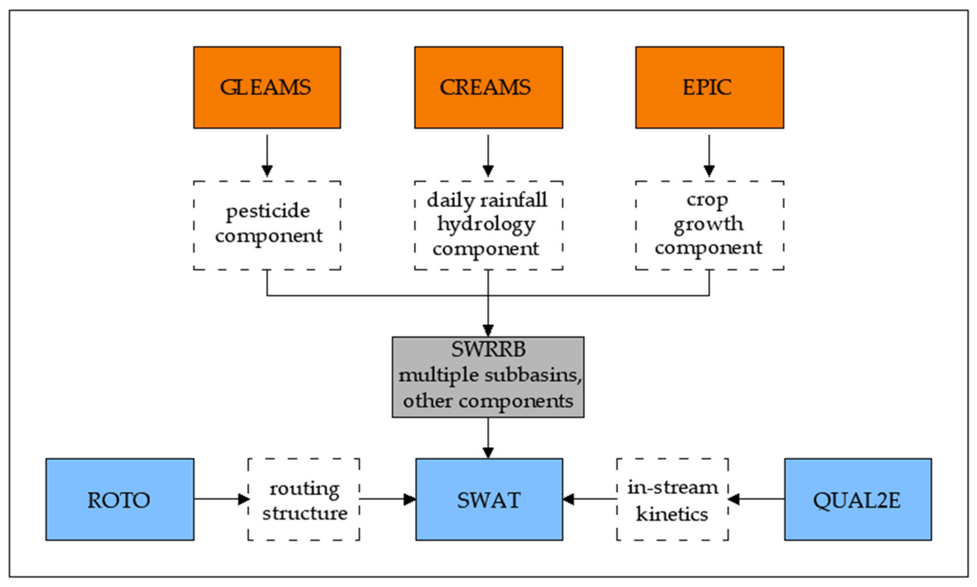
The development of the SWAT model itself is a continuation of modelling by the Agricultural Research Service (ARS) of the United States Department of Agriculture, which covers approximately 30 years. Early versions of the model can be traced back to previously developed ARS models that include The Chemicals, Runoff, and Erosion from Agricultural Management Systems (CREAMS) [7], Groundwater Loading Effects of Agricultural Management Systems (GLEAMS) [8], and the Environmental Impact on Climate (EPIC) model [9], which was originally called the Erosion Productivity Impact Calculator [10]. The current SWAT model is a direct descendant of the Simulator for Water Resources in Rural Basins (SWRRB) [11], which was designed to simulate water management impacts and sediment movement in ungauged rural watersheds throughout the United States. The Routing Outputs to Outlet (ROTO) model was developed in the early 1990s to support the assessment of the downstream impact of water management [12] and the incorporation of flow kinetic routines from the QUAL2E model [13], shown schematically in Figure 1.
The SWAT model was developed to quantify the impact of management in large and complex watersheds with different soil types, land uses, and management conditions over a long period. The model is semi-distributive, with the option of working on annual, monthly, or daily time steps [15]. The latter is recommended for the best output results. SWAT can estimate the relative effects of different management scenarios on water quality, sediment, and agricultural chemical yields in large, ungauged catchments [14]. The components of the sub-catchment model can be divided into hydrology, weather, soil temperature, crop growth, nutrients, pesticides, and agricultural management. Simulated hydrologic processes include surface runoff estimated using the SCS curve number or Green–Ampt infiltration equation; percolation modelled with a layered storage routing technique combined with a crack flow model; lateral subsurface flow; groundwater flow to streams from shallow aquifers; potential evapotranspiration by Hargreaves, Priestley–Taylor, and Penman–Monteith methods; snowmelt; transmission losses from streams and water storage; and losses from pounds [4].
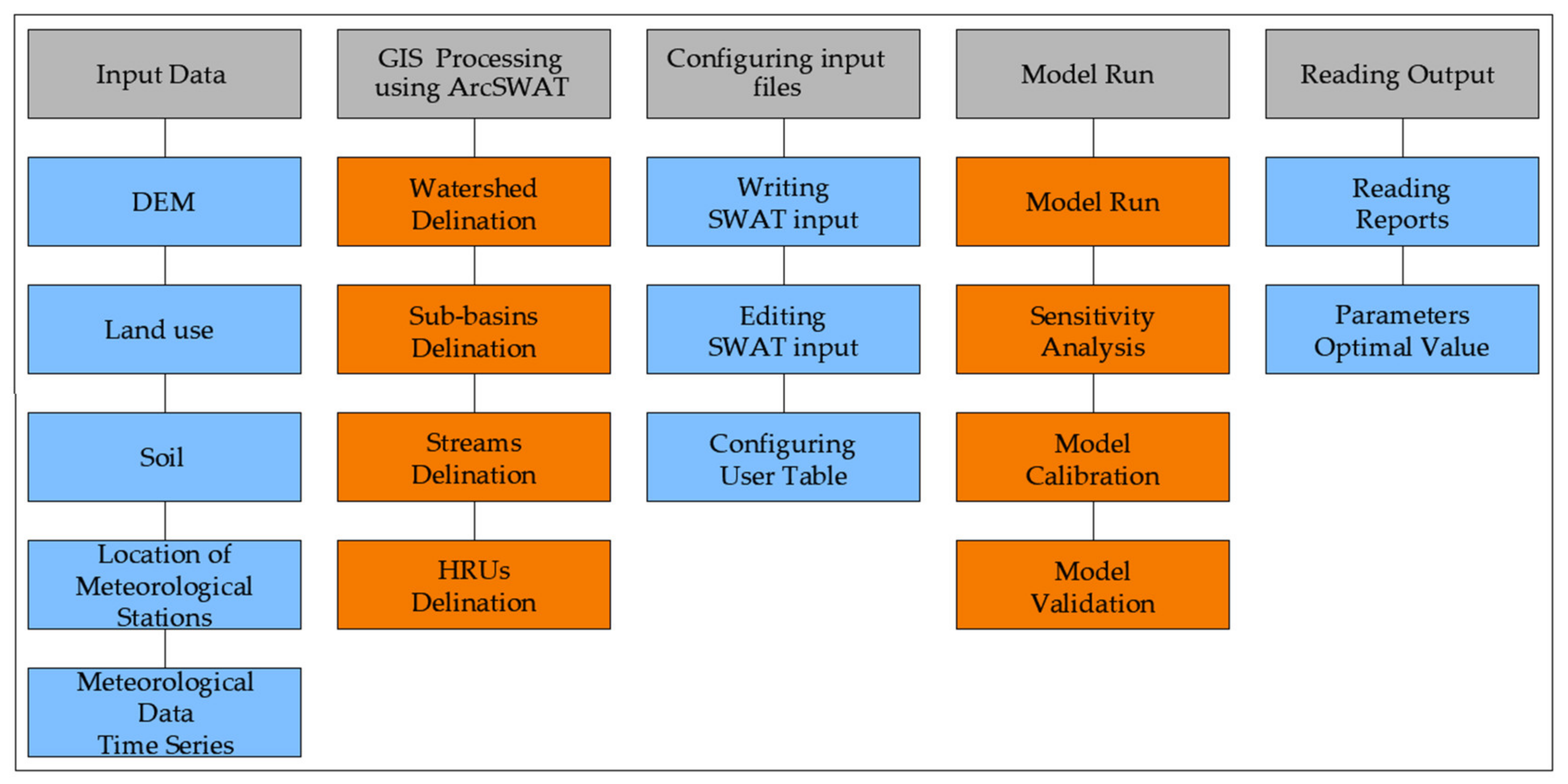
Three key sets of data are required to set up a SWAT model: topography data (digital elevation model, DEM), land use cover, and soil data. Table 1 provides a detailed view of setting up, running, and calibrating the SWAT model, and Figure 2 shows the components of the input/output data. In addition to data on topography, land use, and soil, meteorological data are very important to us for running the SWAT model simulation. The hydrologic cycle is conditioned by the climate and provides moisture and energy inputs, such as daily precipitation, maximum and minimum air temperatures, solar radiation, wind speed, and relative humidity, which control the water balance [16]. SWAT model can read these data directly from the files, and, if something is missing, it can be generated using the SWAT model generator. Snow is calculated when temperatures are below freezing, and soil temperatures are calculated because they affect water movement and the rate of decomposition of soil residues.
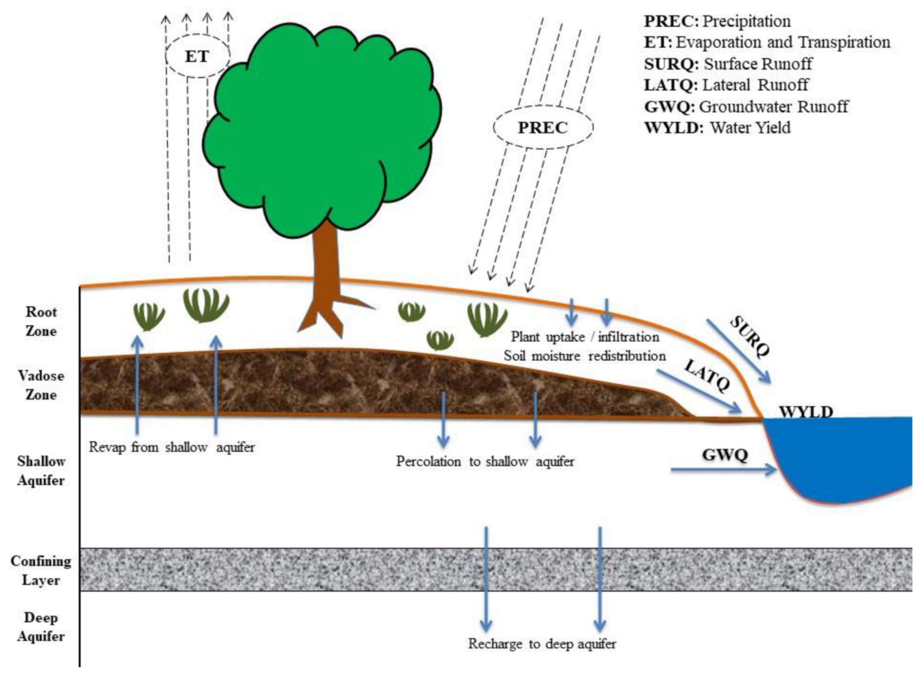
Topographic and land cover data are relatively available on different websites (Earth Explorer site, European Environmental Agency, CORINE Land Cover sites, etc.). Availability of soil data is not so wide outside of USA. Since SWAT was developed in the United States of America, the data used in the model are based on US locations. Therefore, all scientists must find and establish a database of soil characteristics and also for every land cover class spatially distributed in their research area before applying the model because this leads to low simulation accuracy for the research area. The simulation within the SWAT model can be divided into two basic parts. The first simulates processes on the surface of the terrain (surface runoff, amounts of water, sediment, nutrients, and chemical substances in sub-catchment watercourses). The second simulates processes within the watercourse (flow of water, sediment, and other substances from the river network into the basin). The hydrological water cycle process of sub-basins includes hydrology, weather, sediment, soil temperature, plant growth, nutrient pesticides, and agricultural management [4]. The process of the hydrological cycle is shown in Figure 3 which shows the runoff simulation results. The expression for the water balance equation in the SWAT model is [18]:
where SWt is the final water content of the soil, SW0 is the water content in the early stage of the soil, t is time in days, Rday is the daily precipitation, Qsurf is the daily surface runoff, Ea is the daily evapotranspiration (ET), Wseep is the daily percolation, and Qgw is the daily return flow; all units are in mm. When applying the SWAT model, due to different types of land use and different types of soil, the sub-basins are divided into several hydrological response units (HRUs) to improve the accuracy of the simulation.
HRUs are areas of land assumed to respond similarly to weather inputs. HRUs are land units for the land-based portion of the simulated hydrologic cycle, including evapotranspiration, infiltration, percolation, and surface runoff. HRUs are created by overlaying soil, land use, and slope classes within each sub-basin and then deciding how to use these to define HRUs (Figure 3). Using HRU thresholds increases the computational efficiency of SWAT modelling by reducing the number of HRUs but may result in less representative watershed characteristics [14]. HRUs can be developed to reflect fields and other important landscape characteristics, as displayed in Figure 4.
SWAT model input parameters are process-based and must be held within a realistic uncertainty range. The first step in the calibration and validation process with SWAT is the determination of the most sensitive parameters for given watershed or sub-watershed. The user determines which variables adjust based on expert judgment or on sensitivity analysis. Sensitivity analysis is the process of determining the rate of change in the output model with respect to changes in model inputs (parameters). This first step helps determine the predominant processes for the component of interest. There are two types of sensitivity analysis: local, by changing values one at a time, and global, by allowing all parameter values to change. Those two analyses can provide different results because sensitivity of one parameter often depends on the value of other related parameters, and the problem with one-at-a-time analysis is that the correct values of other parameters are fixed and never known. The disadvantage of the global sensitivity analysis is that it requires a large number of simulations. Both procedures provide insight into the sensitivity of the parameters and are necessary steps in model calibration. The next step is calibration. Calibration is an effort to better parameterize the model according to a given set of local conditions, thus reducing the uncertainty of the prediction. It is pre-formed by carefully choosing values for the model input parameters (within their respective uncertainty ranges) by comparing the model predictions for a given set of assumed conditions with observed data for the same conditions. The last step is validation for component of interest (stream flow, sediment yield, etc.). Model validation is the process of demonstrating that a given site-specific model is capable of making sufficiently accurate simulations, although ‘sufficiently accurate’ can vary based on project goals [20]. Validation involves running a model using parameters that were determined during the calibration process and comparing the predictions to observed data not used in the calibration. Calibration can be accomplished manually or using autocalibration tools in SWAT [21] or SWAT-CUP [22]. A good example based on the calibration process involves the streamflow process in which the water balance is contained in the terrestrial phase of hydrology, including evapotranspiration, lateral flow, surface runoff, return flow, tile flow (if present), channel transmission losses, and deep aquifer recharge. Sediments, nutrients, pesticides, and bacteria should also be considered. If a longer time period is available for hydrology than water quality data, it is important to use all available hydrologic data for calibration and validation to achieve long-term trends. This calibration should be completed at the sub-basin or landscape level to account for the variability in the predominant processes for each of the sub-basins involved rather than determining global (basin-wide) processes. Users should check the water balance components (ET, evaporation, surface (base flow ratios, tile flow, proportions, plant yield, and biomass) during the calibration process to make sure the predictions are reasonable for the study region or watershed. Because plant growth and biomass production can have an effect on the water balance, erosion, and nutrient yields, reasonable local/regional plant growth days and biomass production should be verified during model calibration to the extent possible [22].
It is also important to discuss applications of other hydrological models that have similar functionalities as SWAT model. There will be two models presented: HEC-HMS and HEC-RAS model [23,24,25,26]. HEC-HMS is a hydrologic modelling program that allows to establish rainfall–runoff relationships based on watershed characteristics. On the other hand, HEC-RAS is used to make hydraulic models that include rivers and pipes. They have complementary functionalities. The HEC-HMS program is responsible for the hydrological studies. It generates hydrographs that serve as boundary conditions in hydraulic models. In the HEC-HMS program, the hydrograph is calculated with the basin and precipitation data. After this, the results can be exported to different formats for further work in the other information systems.
However, the HEC-RAS program can be basically used in hydraulic modelling. In addition, it allows delineation of flood plains, dam break analysis, and modelling of hydraulic structures, such as bridges and culverts. Within the HEC-RAS program, the entire hydraulic calculation is carried out and the results of draught and velocities are obtained. After this, the results can be exported to ArcGIS to process them and obtain the flood and risk maps.
3. Results
SWAT model application has three large hydrological and environmental research areas: runoff simulation, non-point source pollution, and hydrological impacts under changing environments.
3.1. Runoff Simulation
Runoff in watersheds is a combination of geographical (topographic) and anthropogenic factors. Runoff modelling is critical for studying different complex hydrological processes worldwide, such as snowmelt, flood risk, and pollution risk. Most research has been conducted to establish the parameters of individual watersheds using historical data and a specific time series and using models for predicting future runoff [16]. The Soil Conservation Service Curve Number (SCS-CN) and Green–Ampt infiltration method are two methods for detecting surface influence. As previously stated, runoff is closely linked to topography. Research has focused on the implications of various DEM resolutions on runoff simulations. The results indicate that runoff simulations are proportional to DEM resolution changes, and different runoff volume values were obtained [27,28]. Furthermore, because of the risk of floods induced by monsoons or other precipitation events, the SWAT model is often applied to study watersheds, such as the model of the Subarnarekha River basin in India [29]. Floods are becoming more common due to melting snow induced by the rising air temperature. Data, model structures, forecasts, early warnings, and estimates are described, and it is concluded that most snow models do not have models for blowing snow or frozen ground that could improve the accuracy of snowmelt simulations. Additionally, the incidence of rain on snow is increasing as the climate warms. The observation and simulation of rain and snow processes should be further studied to improve the calibration and validation of snow-melting models [30]. Studies have been conducted on peak flows using a combination of SWAT and machine learning methods. This can reduce the uncertainty of simulations and play an important role in reducing the risk of mountain floods [31].
3.2. Non-Point Source Pollution
Pollution is a factor that threatens ecosystems. Several causes lead to NPS (non-point source) pollution, including soil erosion caused by water in the watershed, usage of pesticides and fertilisers in agricultural areas, disposal of rural livestock manure and garbage, and surface runoff in urban and mining areas. These result in various types of pollution in the form of salts, heavy metals, and organic substances. The SWAT model is suitable for various simulations of NPS pollution, including the pollution load itself, its distribution in space and time, the determination of critical sources of pollution, and the setting of various measures to choose the best management practices for reducing, controlling, and managing pollution [16]. Most SWAT model applications deal with pollution caused by nitrogen and phosphorus. For example, in a study in the Baha River basin, Northwest China, eight different landscape management practices were implemented to reduce NPS loads. The results demonstrate that the intensity of nitrogen and phosphorus pollution losses is correlated with the distribution of precipitation and runoff to a certain extent.
In contrast, the loss of phosphorus load is proportional to the intensity of sediment loss, and it was confirmed that the agricultural area is the main source of pollution and that the effect of reducing the return of agricultural land to the forest area on slopes above 15° proved to be the best practice of landscape management, achieving reduction rates of nitrogen and phosphorus pollution load by 25% [32]. In addition to pollution in landscaping, studies have indicated that nitrogen pollution can lead to the eutrophication of water bodies, and high concentrations of nitrates in drinking water can represent a potential health problem [33]. In the coastal basin of the Yamato River in Japan, a survey of nitrogen loading was conducted over a continuous period of 80 years. The peak nitrogen load in the examined watershed was significantly higher than that caused by urbanisation and population growth in European and American countries. This was because the construction of the wastewater treatment system lagged behind the population growth rate in the area. For some countries undergoing urbanisation and population growth stages, this research can help predict possible future environmental problems and take measures in advance [34]. The impacts of climate change on sediment transport, nutrients, and the effectiveness of best management practices have been predicted in the Pearl River basin of the Upper Mississippi River. The results show the state of the sediment load and its pollution and the possible efficiency of their removal [35].
3.3. Hydrological Impacts under Changing Environment
Evaluating the importance of water as a resource for life on Earth is unnecessary since it keeps our natural landscapes vital. Climate change and a growing population pose a serious threat to freshwater resources [36]. SWAT model applications at HIUCE (hydrological impacts under changing environments) and simulations of the model scenarios are mainly used. These include benchmarking methods, historical inversion methods, model prediction methods, extreme land-use methods, and land-use spatial allocations [16]. Several scientists worldwide have used the SWAT model in different watersheds to analyse the hydrological impacts of environmental change [28,29,30,31,32,33,34,35,36,37,38]. Most of them have studied hydrological impacts due to environmental changes, such as the isolated impacts of climate change or land use change. For example, in a study on the Tapa River basin in India using the SWAT model, the impact of land use change was studied by analysing four maps corresponding to 1975, 1990, 2000, and 2016. From 1975 to 2016, agricultural areas increased by 18%, while forest and pasture areas decreased by 7% and 10%, respectively. This increased surface runoff by approximately 36% and water and sediment yields by approximately 22% [39].
In a similar study in the lower Yom River basin in Thailand, in addition to the increase in surface runoff and sediment yield, there was an increase in pollution in the upper and middle parts of the observed area of approximately 100%. In comparison, the increase in phosphorus pollution ranged from 37% to 377% [40]. Changes in land use are proportional to surface runoff, and changes in forests, agriculture, and settlements are the most significant factors affecting surface runoff. Increases in urbanisation, industrialisation, and more intensive agriculture will increase runoff [41,42]. A few studies have considered the impacts of climate change and changes in land use. One of these studies is the Kaptagat forest catchment area of the Sosiani River in the eastern part of Eldoret City. Over time, land use changed due to increased urbanised areas in the watershed, which decreased forests by 11% from 1989 to 2019 [43]. Many scientists have used SWAT to study hydrological impacts in historically changing environments and predict future environmental changes [44,45]. We observed a study in the form of climate change.
A study of the heavily irrigated agricultural basin of the Rio Grande River in the American state of New Mexico analysed water availability under the influence of climate change from 2022 to 2099. The results showed a decrease in reliability regarding the accumulation storage, which would satisfy the need for water in agriculture. The impact of the decline in surface water can be mitigated by increasing the pressure on the burdened groundwater resources. However, the region should be ready to look for slightly saline and moderately saline groundwater alternatives. Fresh groundwater in the regional aquifer is being depleted in the 21st century under warmer and drier conditions [46]. In addition to water availability, the SWAT model has been applied to investigate hydrological responses to land use change in the large Iriri River basin in the eastern Amazon by predicting the future. The results of this study show the serious potential consequences of deforestation on the components of monthly flow and water balance in the Amazon basin. For example, an increase of over 57% in pasture area increased the simulated annual streamflow by 6.5% and significantly impacted evapotranspiration, surface runoff, and percolation. This is why approximately 80% of the Iriri River basin is a legally protected area for conservation strategies in the Brazilian Amazon region [47].
Moreover, soil erosion is one of the most serious impacts of the problem of soil degradation. Changes in the spread of farming on slopes, increased urbanization, and deforestation are just some of the significant issues in hilly and mountainous areas. Areas with transitional zone of forest and agricultural land experience the greatest erosion caused by the action of anthropogenic processes [48]. Additionally, higher flow and intensity of precipitation contribute to the acceleration of soil erosion and increased losses of sediment and nutrients downstream [49]. Natural factors, including heavy rainfall and local soil properties in an erosion-prone landscape, were the underlying factors responsible for high soil erosion in the Sumani basin in West Sumatra, Indonesia. Apart from these causes, changes in land use have accelerated soil erosion, and the rate of soil erosion from 1992 to 2002 showed an increase of 37% due to conversion of forest to agricultural fields (vegetable gardens) [48]. Along with erosion comes the problem of sediment deposition. In a study of the Salma watershed located on the Hari River in western Afghanistan, the SWAT model was used to analyse runoff and sediment output to identify major erosion basins in the Salma dam and assess best management practices for reducing sediment transport to reservoirs in order to extend their usable life. The groundwater delay and groundwater discharge regression for water discharge, soil depth, and Manning’s coefficient of channel roughness for sediment yield were the most sensitive factors. According to the simulation, exclusion fence, streambank stabilization, conservation crop rotation, check dams, brush layering, brush mattress, and terracing can all be utilized to minimize soil erosion and reduce sediment loads in the research areas [50].
4. Discussion
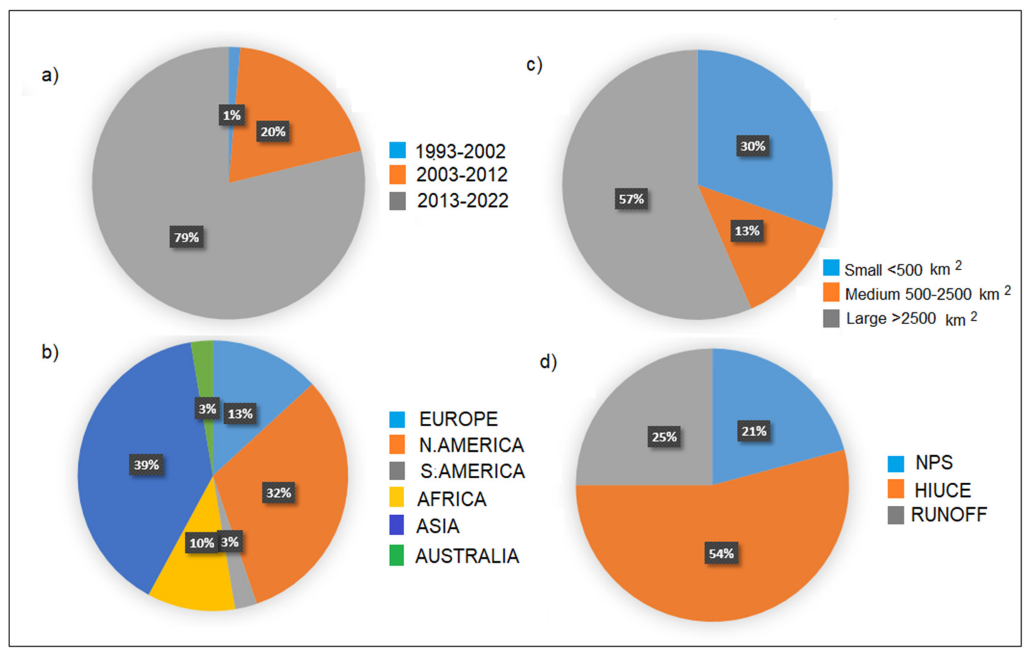
Searching for literature related to the SWAT model on the official website of the SWAT model (https://www.card.iastate.edu/swat_articles/, accessed on 17 February 2023), we can see that more than 5000 scientific articles have been published since its inception in the 1990s. As the model developed from the 1990s until today, we note a significant increase in the number of articles, mainly in the last 10 years. The number of articles has almost reached 4000 scientific articles (Figure 5a).
Despite its wide application, the SWAT model has limitations and weaknesses. Moreover, for the current state of the SWAT model with a large amount of data, there are still some problems and possibilities for improving the same application.
4.1. Weaknesses
One of the problems of the SWAT model is the time series of data to be examined when applying the model itself. Most scientists use annual, seasonal, or monthly data to simulate and test models. Previous studies have shown that the model can be simulated and tested effectively based on a long time series. However, if we want to simulate and test on a daily time series of data, there is a possibility that there will be errors in the model, especially in the daily runoff, if other data series do not correspond [16]. Running the model requires a wide range of data (topography, land cover, soil type and soil characteristics, meteorological data, data on flows, nutrients, sediments, etc.) and modifying them in detail during calibration, which discourages scientists from applying the SWAT model. However, given the complexity of the environment, any neglect or underestimation of the importance of parameters can lead to inaccurate model simulation results and estimates [5]. As stated earlier, SWAT was developed in the USA, and the soil data used in the model were based on the area of the USA. For this reason, all scientists must find and process in detail the database of soil characteristics and land cover in their research area when they want to apply the model because land cover characteristics are also different compared to areas in the USA. In contrast, this leads to low accuracy in the simulation and analysis of the model for the research area [16].
4.2. Strengths
SWAT is a free model that allows scientists to model the amount of surface water worldwide. This model deals with the connection between surface terrestrial and channel ecological processes, studies water quantity, water quality, and climate change, and offers simulations and analyses of different watershed sizes on an annual, seasonal, monthly, or daily basis over long periods. The 30-year model development period resulted in the creation of several new interfaces and tools to support the model. The SWAT editor is a stand-alone program used for editing input data and running the model. The SWAT-CUP serves for sensitivity analysis, calibration, validation, and uncertainty analysis of the SWAT model. One of its advantages is that it enables the simulation of human activities and agricultural measures. In most cases, they are directly related to changes in the model parameters. Crop rotations, fertilizer rates, the timing of fertilizer application, and tillage, sowing, and harvesting time can be modelled using Management files. For these reasons, the SWAT model has wide applications worldwide. However, most applications come from North America as its dominant continent and Asia, namely China (Figure 5b). The model is often used in research on watersheds larger than 2500 km2 (57%). However, a portion of the SWAT application on watersheds smaller than 500 km2 is also significant (30%) (Figure 5c).
According to the articles published in the past 5–10 years, most of them dealt with hydrological impacts under environmental change (54%), the simulation of runoff (25%), and NPS pollution (21%) (Figure 5d). Climate change is a global problem with many significant impacts on the environment, such as the quality and quantity of water resources, water balance, and biodiversity. Scientists are aware of this serious problem and the daily efforts to stop or slow down climate change impacts. Therefore, the SWAT model is a good tool for analysing, predicting, and managing hydrological impacts under environmental change.
Some of the discussed weaknesses are overcome in the SWAT+ model, developed in recent years in order to ensure far more advanced functions and capacities to handle challenging watershed modelling tasks for hydrologic and water quality processes [51,52]. Some of the most pronounced strengths are its construction consisting of independent modules, new functionalities of aquifers and reservoir operation rules, corresponding aquifer boundaries able to be defined flexibly without following the limitations by HRUs, and higher flexibility in representing agricultural practices [53]. Future development of SWAT+ is expected to improve hydrological simulations in climate change and environment conditions.
Our analysis of the SWAT model shows its suitability for application in the conditions of changing climate and environment, which validates many articles published in the last 5–10 years. Changes in hydrological processes have become more pronounced in this century, which makes the SWAT model more interesting due to its strengths and despite its weaknesses.
5. Conclusions
The wide range of SWAT applications that have been described here shows us that the SWAT model is a very flexible and robust tool that can be used to simulate a variety of watershed problems. Currently, studies on this model are mainly focusing on the application of the model, the accuracy of the model, and model coupling. The largest areas of application of the model are runoff simulation, hydrological impact under changing environment, non-point source pollution, and soil erosion. Most modelers struggle with input data, so it is important to note that the process of configuring SWAT models for watersheds has been greatly facilitated by the development of GIS-based interfaces that allow us straightforward means of translating digital land use, topographic, and soil data into model inputs. The SWAT model and its GIS interfaces aid the water resources professional in basin-scale studies of water availability and water quality and help to reduce the time and cost necessary to conduct such studies several-fold compared to other distributed parameter models. In addition to the advantages, there are also threats that can negatively affect the performance and use of the model if they are not addressed. In the process of creating the model, it is necessary to make several parameter adjustments to improve simulation. These adjustments are not measurable and are completed using the experience of the modeler, his knowledge, and subjective assessment of the research area. This can have important implications for the overall performance and outcome of the model and its suitability for particular case studies, which is difficult to quantify. Moreover, it is important to note that, in a highly managed watershed, unknown activities, such as construction site transportation, water abstraction, reservoirs, dams, waste treatment plants, and waste and dumping of chemicals into rivers, can contribute to significant error in model results. Spatial resolution of land use, soil, slope, and weather data are usually not set on the same scale. This leads us to the conclusion that spatial results are as good as the data with the lowest resolution. Distribution of crops on site, crop rotation, and management practices (sowing and harvesting dates and fertilizer application dates) are a major spatial representation challenge in large- and medium-sized watersheds. Combined with uncertainties in the soil spatial and attribute data, they may significantly affect proper modelling of water balance and sediment transport in the catchments.
Author Contributions
Conceptualization, J.J. and L.T.; methodology, J.J.; validation, L.T.; formal analysis, J.J.; writing—original draft preparation, J.J. and L.T.; writing—review and editing, J.J. and L.T.; visualization, J.J.; supervision, L.T. All authors have read and agreed to the published version of the manuscript.
Funding
This research received no external funding.
Data Availability Statement
Publicly available datasets were analyzed in this study.
Conflicts of Interest
The authors declare no conflict of interest.
References
- Volk, M.; Liersch, S.; Schmidt, G. Towards the implementation of the European Water Framework Directive? Lessons learned from water quality simulations in an agricultural watershed. Land Use Policy 2009, 26, 580–588. [Google Scholar] [CrossRef]
- Hejzlar, J.; Anthony, S.; Arheimer, B.; Behrendt, H.; Bouraoui, F.; Grizzetti, B.; Groenendijk, P.; Jeuken, M.H.J.L.; Johnsson, H.; Porto, A.L.; et al. Nitrogen and phosphorus retention in surface waters: An inter-comparison of predictions by catchment models of different complexity. J. Environ. Monit. 2009, 11, 584–593. [Google Scholar] [CrossRef] [PubMed]
- Chow, V.T.; Maidment, D.R.; Mays, L.W. Applied Hydrology; McGraw-Hill, Inc.: New York, NY, USA, 1988; p. 572. [Google Scholar]
- Arnold, J.G.; Srinivasan, R.; Muttiah, R.S.; Williams, J.R. Large area hydrologic modeling and assessment. Part 1: Model development. J. Am. Water Resour. Assoc. 1998, 34, 73–89. [Google Scholar] [CrossRef]
- Glavan, M.; Pintar, M. Strengths, Weaknesses, Opportunities and Threats of Catchment Modelling with Soil and Water Assessment Tool (SWAT) Model. In Water Resources Management and Modeling; InTechOpen: Rijeka, Croatia, 2015. [Google Scholar]
- Srinivasan, R.; Zhang, X.; Arnold, J. SWAT ungauged: Hydrological budget and crop yield predictions in the upper Mississippi River basin. Trans. ASABE 2010, 53, 1533–1546. [Google Scholar] [CrossRef]
- Knisel, W.G. CREAMS: A Field-Scale Model for Chemicals, Runoff, and Erosion from Agricultural Management Systems; United States Department of Agriculture, Science and Education Administration: Washington, DC, USA, 1982. [Google Scholar]
- Leonard, R.A.; Knisel, W.G.; Still, D.A. Gleams: Groundwater Loading Effects of Agricultural Management Systems. Trans. Am. Soc. Agric. Eng. 1987, 30, 1403–1418. [Google Scholar] [CrossRef]
- Izaurralde, R.C.; Williams, J.R.; McGill, W.B.; Rosenberg, N.J.; Jakas, M.C.Q. Simulating soil C dynamics with EPIC: Model description and testing against long-term data. Ecol. Model. 2006, 192, 362–384. [Google Scholar] [CrossRef]
- Williams, J.R. The erosion-productivity impact calculator (EPIC) model: A case history. Philos. Trans. R. Soc. B: Biol. Sci. 1990, 329, 421–428. [Google Scholar]
- Arnold, J.G.; Williams, J.R. Validation of Swrrb—A Simulator for Water Resources in Rural Basins. J. Water Resour. Plan. Manag. 1985, 113, 107–114. [Google Scholar] [CrossRef]
- Arnold, B.J.G.; Williams, J.R.; Maidment, D.R. Continuous-Time Water and Sediment-Routing Model for Large Basins. J. Hydraul. Eng. 1995, 121, 171–183. [Google Scholar] [CrossRef]
- Brown, L.C.; Barnwell, T.O. The Enhanced Stream Water Quality Models Qual2E and Qual2E-UNCAS Documentation and User Manual; US Environmental Protection Agency, Office of Research and Development, Environmental Research Laboratory: Athens, GA, USA, 1987; p. 189. [Google Scholar]
- PW Gassman, M.R.; Reyes, C.H.; Green, J.G. Arnold. The Soil and Water Assessment Tool: Historical Development, Applications, and Future Research Directions. Trans. ASABE 2007, 50, 1211–1250. [Google Scholar] [CrossRef]
- Douglas-Mankin, K.R.; Srinivasan, R.; Arnold, J.G. Soil and Water Assessment Tool (Swat) Model: Current Developments and Applications. Trans. ASABE 2010, 53, 1423–1431. [Google Scholar] [CrossRef]
- Wang, Y.; Jiang, R.; Xie, J.; Zhao, Y.; Yan, D.; Yang, S. Soil and Water Assessment Tool (SWAT) Model: A Systemic Review. J. Coast. Res. 2019, 93, 22–30. [Google Scholar] [CrossRef]
- Diwakar, S.K.; Kaur, D.S.; Patel, D.N. Hydrologic Assessment in a Middle Narmada Basin, India using SWAT Model. Int. J. Eng. Technol. Comput. Res. 2014, 2, 10–25. [Google Scholar]
- Li, B.Q.; Xiao, W.H.; Wang, Y.C.; Yang, M.Z.; Huang, Y. Impact of land use/cover change on the relationship between precipitation and runoff in typical area. J. Water Clim. Chang. 2018, 9, 261–274. [Google Scholar] [CrossRef]
- Wang, Z.; Cao, J.; Yang, H. Multi-time scale evaluation of forest water conservation function in the semiarid mountains area. Forests 2021, 12, 116. [Google Scholar] [CrossRef]
- Refsgaard, J.C. Parameterisation, calibration and validation of distributed hydrological models. J. Hydrol. 1997, 198, 69–97. [Google Scholar] [CrossRef]
- Van Griensven, A.; Bauwens, W. Multiobjective autocalibration for semidistributed water quality models. Water Resour. Res. 2003, 39, 1–9. [Google Scholar] [CrossRef]
- Arnold, J.G.; Moriasi, D.N.; Gassman, P.W.; Abbaspour, K.C.; White, M.J.; Srinivasan, R.; Santhi, C.; Harmel, R.D.; Van Griensven, A.; Van Liew, M.W.; et al. SWAT: Model use, calibration, and validation. Trans. ASABE 2012, 55, 1491–1508. [Google Scholar] [CrossRef]
- Kiesel, J.; Schmalz, B.; Brown, G.L.; Fohrer, N. Application of a hydrological-hydraulic modelling cascade in lowlands for investigating water and sediment fluxes in catchment, channel and reach. J. Hydrol. Hydromech. 2013, 61, 334–346. [Google Scholar] [CrossRef]
- Chathuranika, I.M.; Gunathilake, M.B.; Baddewela, P.K.; Sachinthanie, E.; Babel, M.S.; Shrestha, S.; Jha, M.K.; Rathnayake, U.S. Comparison of Two Hydrological Models, HEC-HMS and SWAT in Runoff Estimation: Application to Huai Bang Sai Tropical Watershed, Thailand. Fluids 2022, 7, 267. [Google Scholar] [CrossRef]
- Pistocchi, A.; Mazzoli, P. Use of HEC-RAS and HEC-HMS models with ArcView for hydrologic risk management. In Proceedings of the International Congress on Environmental Modelling and Software, Lugano, Switzerland, 1 June 2002. [Google Scholar]
- AL-Hussein, A.A.M.; Khan, S.; Ncibi, K.; Hamdi, N.; Hamed, Y. Flood Analysis Using HEC-RAS and HEC-HMS: A Case Study of Khazir River (Middle East—Northern Iraq). Water 2022, 14, 3779. [Google Scholar] [CrossRef]
- Lin, S.; Jing, C.; Chaplot, V.; Yu, X.; Zhang, Z.; Moore, N.; Wu, J. Effect of DEM resolution on SWAT outputs of runoff, sediment and nutrients. Hydrol. Earth Syst. Sci. Discuss. 2010, 7, 4411–4435. Available online: http://www.hydrol-earth-syst-sci-discuss.net/7/4411/2010/ (accessed on 20 February 2017).
- Nagaveni, C.; Kumar, K.P.; Ravibabu, M.V. Evaluation of TanDEMx and SRTM DEM on watershed simulated runoff estimation. J. Earth Syst. Sci. 2019, 128, 2. [Google Scholar] [CrossRef]
- Yaduvanshi, A.; Sharma, R.K.; Kar, S.C.; Sinha, A.K. Rainfall–runoff simulations of extreme monsoon rainfall events in a tropical river basin of India. Nat. Hazards 2018, 90, 843–861. [Google Scholar] [CrossRef]
- Zhou, G.; Cui, M.; Wan, J.; Zhang, S. A review on snowmelt models: Progress and prospect. Sustainability 2021, 13, 11485. [Google Scholar] [CrossRef]
- Senent-Aparicio, J.; Jimeno-Sáez, P.; Bueno-Crespo, A.; Pérez-Sánchez, J.; Pulido-Velázquez, D. Coupling machine-learning techniques with SWAT model for instantaneous peak flow prediction. Biosyst. Eng. 2019, 177, 67–77. [Google Scholar] [CrossRef]
- Li, S.; Li, J.; Xia, J.; Hao, G. Optimal control of nonpoint source pollution in the Bahe River Basin, Northwest China, based on the SWAT model. Environ. Sci. Pollut. Res. 2021, 28, 55330–55343. [Google Scholar] [CrossRef]
- Zheng, M.; Sheng, Y.; Sun, R.; Tian, C.; Zhang, H.; Ning, J.; Sun, Q.; Li, Z.; Bottrell, S.H.; Mortimer, R.J. Identification and Quantification of Nitrogen in a Reservoir, Jiaodong Peninsula, China. Water Environ. Res. 2017, 89, 369–377. [Google Scholar] [CrossRef]
- Wang, K.; Onodera, S.I.; Saito, M. Evaluation of nitrogen loading in the last 80 years in an urbanized Asian coastal catchment through the reconstruction of severe contamination period. Environ. Res. Lett. 2022, 17, 014010. [Google Scholar] [CrossRef]
- Jayakody, P.; Parajuli, P.B.; Cathcart, T.P. Impacts of climate variability on water quality with best management practices in sub-tropical climate of USA. Hydrol. Process. 2014, 28, 5776–5790. [Google Scholar] [CrossRef]
- King, E.A.; Paget, M.J.; Briggs, P.R.; Raupach, M.R.; Trudinger, C.M. Operational Delivery of Hydro-Meteorological Monitoring and Modeling Over the Australian Continent. IEEE J. Sel. Top. Appl. Earth Obs. Remote. Sens. 2009, 2, 241–249. [Google Scholar] [CrossRef]
- Naz, R.; Ashraf, A.; Van der Tol, C.; Aziz, F. Modeling hydrological response to land use/cover change: Case study of Chirah Watershed (Soan River), Pakistan. Arab. J. Geosci. 2020, 13, 1220. [Google Scholar] [CrossRef]
- Said, M.; Hyandye, C.; Mjemah, I.C.; Komakech, H.C.; Munishi, L.K. Evaluation and Prediction of the Impacts of Land Cover Changes on Hydrological Processes in Data Constrained Southern Slopes of Kilimanjaro, Tanzania. Earth 2021, 2, 225–247. [Google Scholar] [CrossRef]
- Munoth, P.; Goyal, R. Impacts of land use land cover change on runoff and sediment yield of Upper Tapi River Sub-Basin, India. Int. J. River Basin Manag. 2020, 18, 177–189. [Google Scholar] [CrossRef]
- Chotpantarat, S.; Boonkaewwan, S. Impacts of land-use changes on watershed discharge and water quality in a large inten-sive agricultural area in Thailand. Hydrol. Sci. J. 2018, 63, 1386–1407. [Google Scholar] [CrossRef]
- Astuti, I.S.; Sahoo, K.; Milewski, A.; Mishra, D.R. Impact of Land Use Land Cover (LULC) Change on Surface Runoff in an Increasingly Urbanized Tropical Watershed. Water Resour. Manag. 2019, 33, 4087–4103. [Google Scholar] [CrossRef]
- Ma, K.; Huang, X.; Liang, C.; Zhao, H.; Zhou, X.; Wei, X. Effect of land use/cover changes on runoff in the Min River water-shed. River Res. Appl. 2020, 36, 749–759. [Google Scholar] [CrossRef]
- Kibii, J.K.; Kipkorir, E.C.; Kosgei, J.R. Application of soil and water assessment tool (SWAT) to evaluate the impact of land use and climate variability on the Kaptagat catchment river discharge. Sustainability 2021, 13, 1802. [Google Scholar] [CrossRef]
- Getu Engida, T.; Nigussie, T.A.; Aneseyee, A.B.; Barnabas, J. Land Use/Land Cover Change Impact on Hydrological Process in the Upper Baro Basin, Ethiopia. Appl. Environ. Soil Sci. 2021, 2021, 6617541. [Google Scholar] [CrossRef]
- Awotwi, A.; Anornu, G.K.; Quaye-Ballard, J.A.; Annor, T.; Forkuo, E.K.; Harris, E.; Agyekum, J.; Terlabie, J.L. Water balance responses to land-use/land-cover changes in the Pra River Basin of Ghana, 1986–2025. Catena 2019, 182, 104129. [Google Scholar] [CrossRef]
- Samimi, M.; Mirchi, A.; Townsend, N.; Gutzler, D.; Daggubati, S.; Ahn, S.; Sheng, Z.; Moriasi, D.; Granados-Olivas, A.; Alian, S.; et al. Climate Change Impacts on Agricultural Water Availability in the Middle Rio Grande Basin. JAWRA J. Am. Water Re-sour. Assoc. 2022, 58, 164–184. [Google Scholar] [CrossRef]
- Dos Santos, V.; Laurent, F.; Abe, C.; Messner, F. Hydrologic response to land use change in a large basin in eastern Amazon. Water 2018, 10, 429. [Google Scholar] [CrossRef]
- Saidi, A.; Indra, R.; Somura, H.; Wakatsuki, T.; Masunaga, T. Soil erosion characterization in an agricultural watershed in West Sumatra, Indonesia. Tropics 2010, 19, 29–42. [Google Scholar]
- Li, M.; Shi, X.; Shen, Z.; Yang, E.; Bao, H.; Ni, Y. Effect of hillslope aspect on landform characteristics and erosion rates. Environ Monit Assess. Environ. Monit. Assess. 2019, 191, 598. [Google Scholar] [CrossRef]
- Sadiqi, S.S.J.; Hong, E.M.; Nam, W.H. Identification of priority management practices for soil erosion control through estimation of runoff and sediment yield using soil and water assessment tool on Salma watershed in Afghanistan. Irrig. Drain. 2022, 71, 804–822. [Google Scholar] [CrossRef]
- Bieger, K.; Arnold, J.G.; Rathjens, H.; White, M.J.; Bosch, D.D.; Allen, P.M.; Volk, M.; Srinivasan, R. Introduction to SWAT+, A Completely Restructured Version of the Soil and Water Assessment Tool. J. Am. Water Resour. Assoc. 2017, 53, 115–130. [Google Scholar] [CrossRef]
- Yen, H.; Park, S.; Arnold, J.G.; Srinivasan, R.; Chawanda, C.J.; Wang, R.; Feng, Q.; Wu, J.; Miao, C.; Bieger, K.; et al. IPEAT+: A built-in optimization and automatic calibration tool of SWAT+. Water 2019, 11, 1681. [Google Scholar] [CrossRef]
- Nkwasa, A.; Chawanda, C.J.; Msigwa, A.; Komakech, H.C.; Verbeiren, B.; van Griensven, A. How can we represent seasonal land use dynamics in SWAT and SWAT+ models for African cultivated catchments. Water 2020, 12, 1541. [Google Scholar] [CrossRef]
Figure 1.
Schematic of SWAT developmental history [14].
Figure 1.
Schematic of SWAT developmental history [14].

Figure 2.
Components’ input/output data of SWAT model [17].
Figure 2.
Components’ input/output data of SWAT model [17].

Figure 3.
The hydrological cycle process of the SWAT model [19].
Figure 3.
The hydrological cycle process of the SWAT model [19].

Figure 4.
Hydrological response unit (HRU) (https://ecce.esri.ca/blog/unb-blog/2019/12/04/identifying-source-of-nitrate-load-using-swat/), accessed on 27 March 2023).
Figure 4.
Hydrological response unit (HRU) (https://ecce.esri.ca/blog/unb-blog/2019/12/04/identifying-source-of-nitrate-load-using-swat/), accessed on 27 March 2023).

Figure 5.
SWAT model application by number of publications (a), by continent (b), by the size of the watershed (c), and by research problem (d).
Figure 5.
SWAT model application by number of publications (a), by continent (b), by the size of the watershed (c), and by research problem (d).


Table 1.
Model input data for a SWAT model.
| Data Type | Description | |
|---|---|---|
| Set-up | Digital Elevation Model (Topography) | 10, 25, 50, 100 m resolution (most often) |
| Soil characteristics | Raster data as an input for all the spatial data of soil types, Database describing soil profiles and horizons | |
| Land cover | Spatially distributed land cover classes for 1990, 2000, 2006, 2012, and 2018 * | |
| Run | Climate data | Station data for air temperature, precipitation, relative humidity, wind speed, solar radiation |
| Calibration | Biomass | Information about Leaf Area Index for each land cover |
| Discharge data | Mostly less than 20 years of recorded discharge data | |
| Suspended sediment | Suspended sediment discharge | |
| Evapotranspiration | The Soil Evaporation Compensation factor, The Plant Evaporation Compensation factor, The Soil Albedo, The Plant Canopy, etc. | |
| Nutrients concentrations | Monitoring of concentrations of nitrogen or phosphate compounds in surface waters at the station |
* available years on the official website of CORINE Land Cover for land cover data mostly used for European countries.
Disclaimer/Publisher’s Note: The statements, opinions and data contained in all publications are solely those of the individual author(s) and contributor(s) and not of MDPI and/or the editor(s). MDPI and/or the editor(s) disclaim responsibility for any injury to people or property resulting from any ideas, methods, instructions or products referred to in the content. |
© 2023 by the authors. Licensee MDPI, Basel, Switzerland. This article is an open access article distributed under the terms and conditions of the Creative Commons Attribution (CC BY) license (https://creativecommons.org/licenses/by/4.0/).
Share and Cite
MDPI and ACS Style
Janjić, J.; Tadić, L. Fields of Application of SWAT Hydrological Model—A Review. Earth 2023, 4, 331-344. https://doi.org/10.3390/earth4020018
AMA Style
Janjić J, Tadić L. Fields of Application of SWAT Hydrological Model—A Review. Earth. 2023; 4(2):331-344. https://doi.org/10.3390/earth4020018
Chicago/Turabian StyleJanjić, Josip, and Lidija Tadić. 2023. "Fields of Application of SWAT Hydrological Model—A Review" Earth 4, no. 2: 331-344. https://doi.org/10.3390/earth4020018