
Simulating Urban Growth Using the Cellular Automata Markov Chain Model in the Context of Spatiotemporal Influences for Salem and Its Peripherals, India


Abstract
:1. Introduction
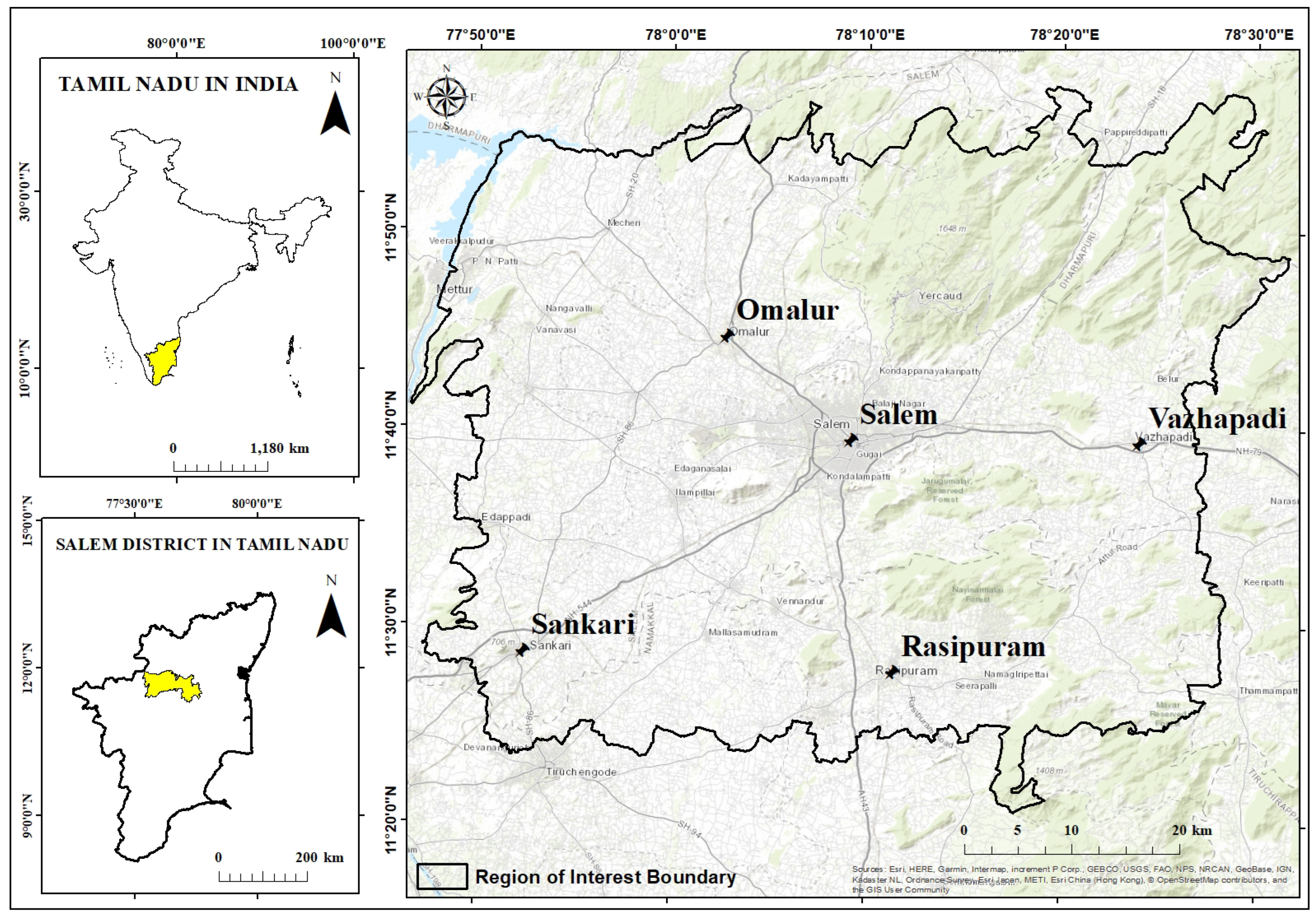
2. Study Area
3. Data and Software
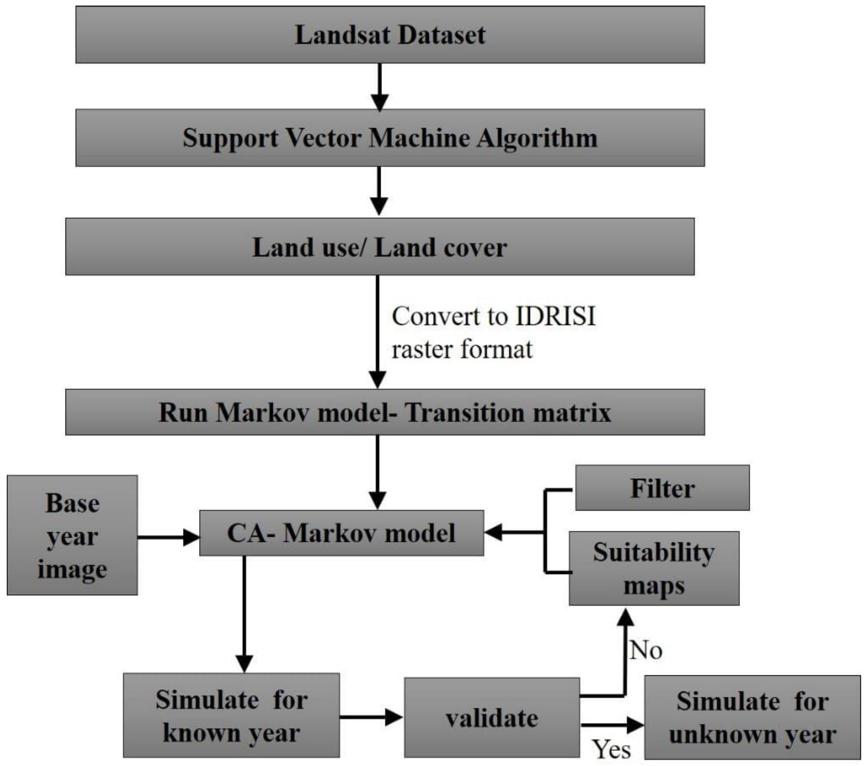
4. Methodology
4.1. Data Preprocessing
4.2. LU/LC Classification
4.3. Accuracy Assessment
4.4. Change Detection and Urban Growth Analysis
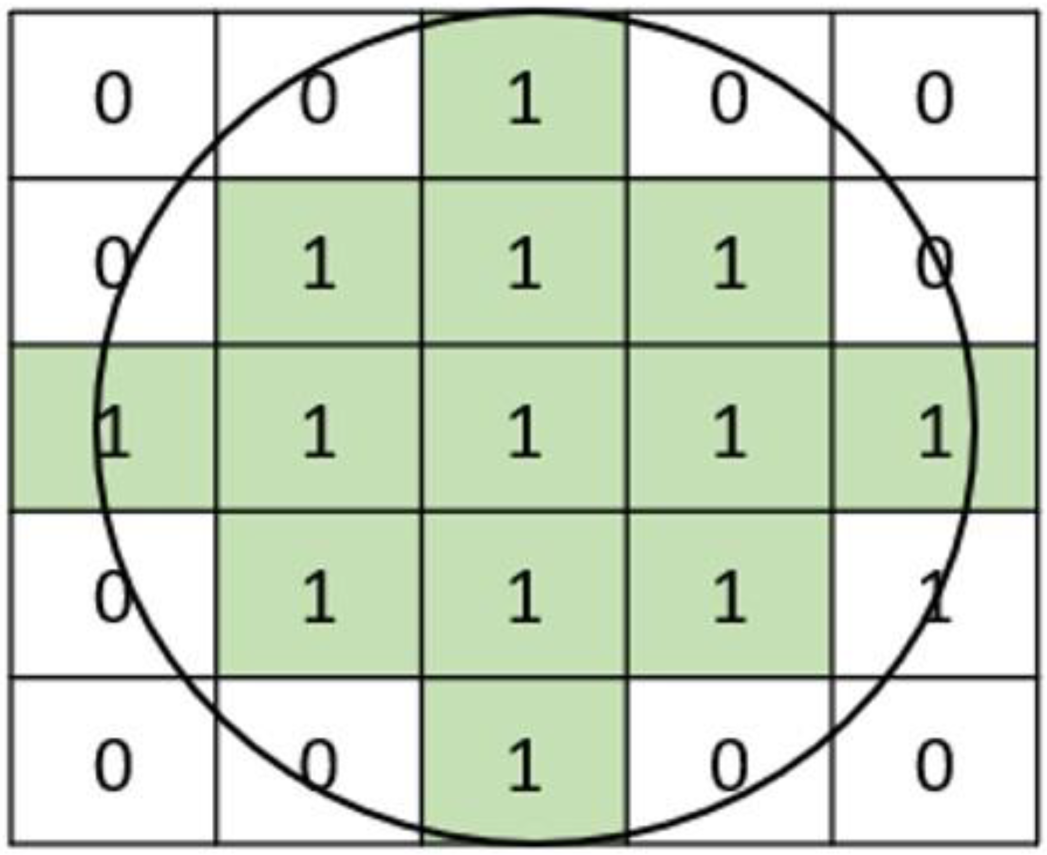
4.5. Hybrid CA–Markov Modeling
5. Results and Discussions
5.1. Classification and Accuracy Assessment
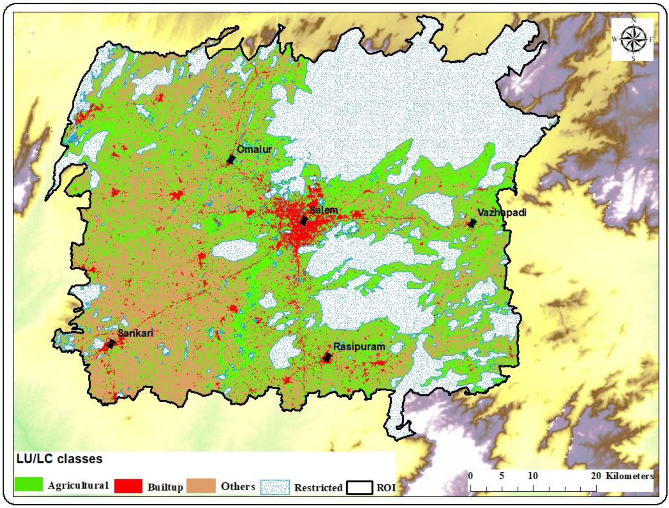
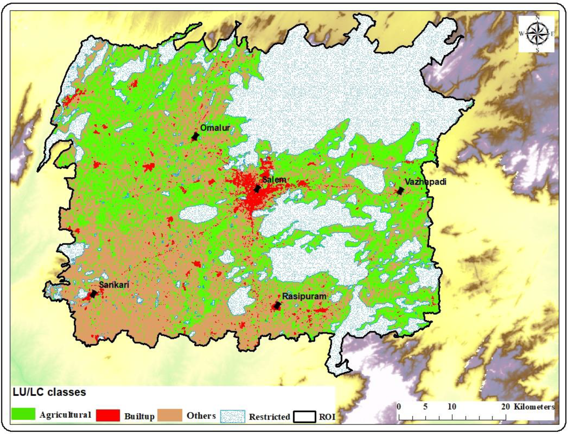
5.2. Time Series Analysis of LU/LC and Urban Growth
5.3. CA–Markov Modeling
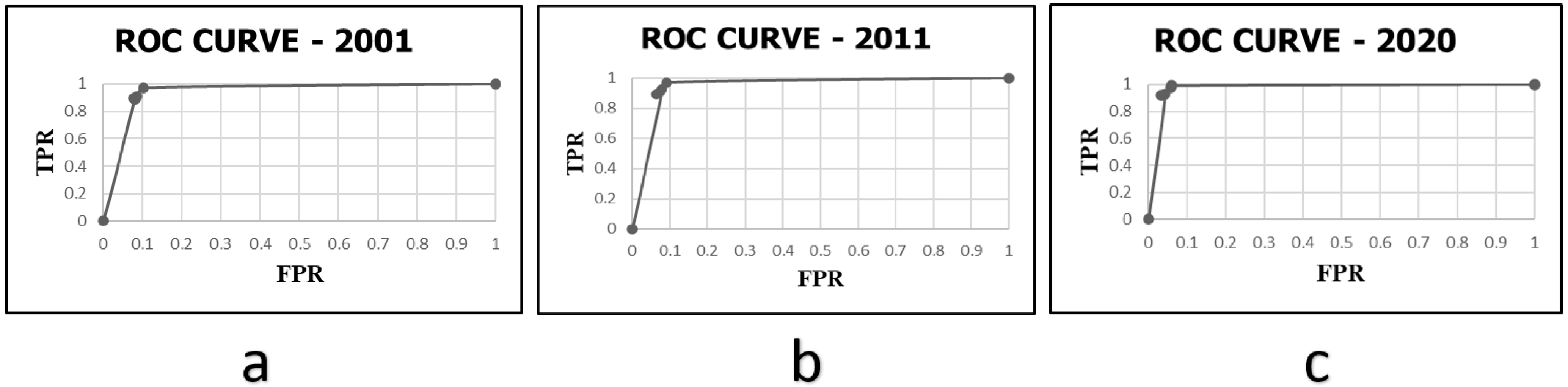
5.4. Model Validation
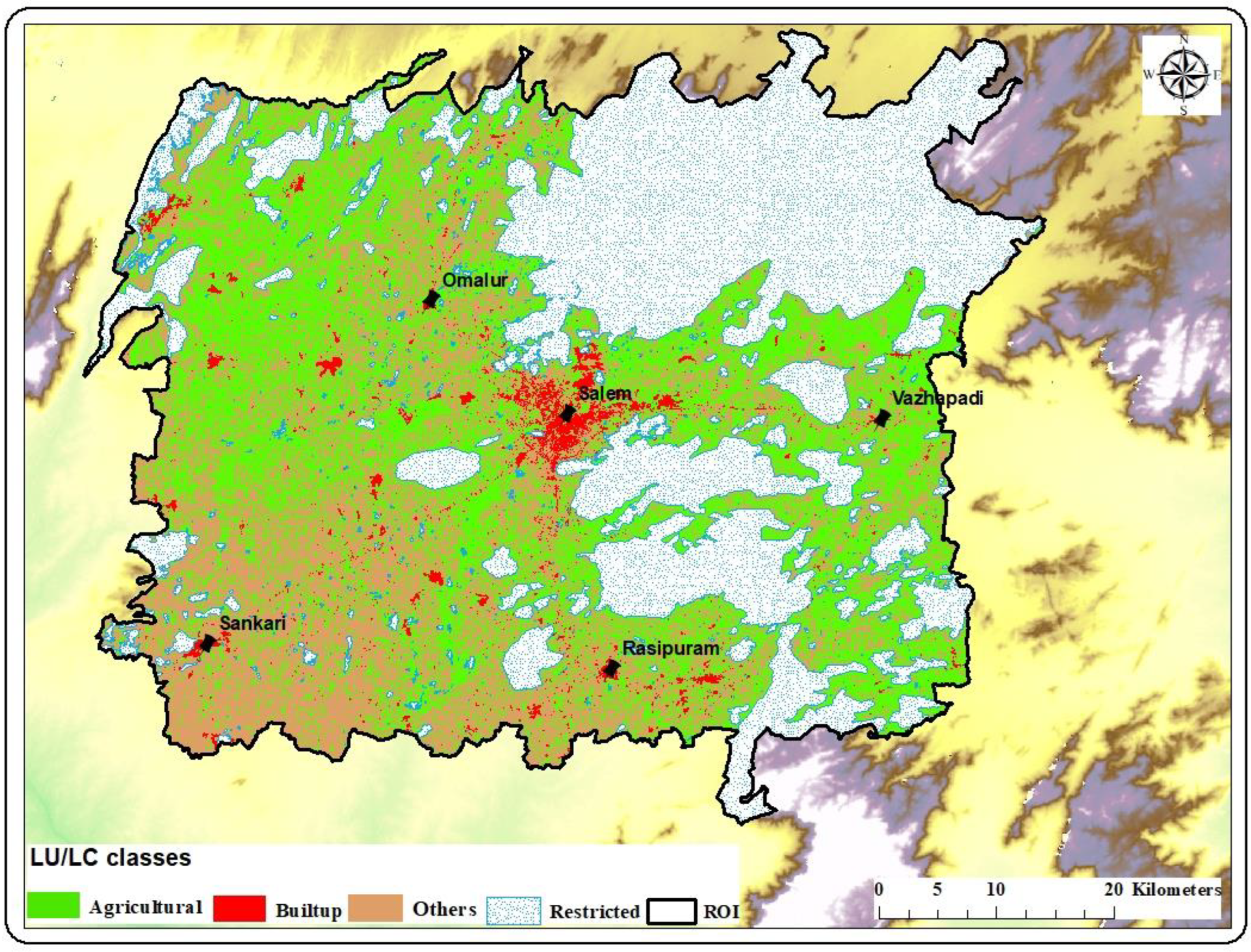
5.5. Prediction of Urban Sprawl
6. Conclusions
Author Contributions
Funding
Institutional Review Board Statement
Informed Consent Statement
Data Availability Statement
Conflicts of Interest
References
- UN Habitat. World Cities Report 2022: Envisaging the Future of Cities. Available online: https://unhabitat.org/sites/default/files/2022/06/wcr_2022.pdf (accessed on 28 February 2022).
- Nouri, J.; Gharagozlou, A.; Arjmandi, A.; Faryadi, S.; Adl, M. Predicting urban land use changes using a CA-Markov model. Arab. J. Sci. Eng. 2014, 39, 5565–5573. [Google Scholar] [CrossRef]
- Anthony, G.O.; Yeh Xia, L.; Chang, X. Cellular Automata Modeling for Urban and Regional Planning. In Urban Informatics; Part of The Urban Book Series; Springer: Singapore, 2021; pp. 865–883. [Google Scholar]
- Maithani, S. A Neural Network based Urban Growth Model of an Indian City. J. Indian Soc. Remote Sens. 2010, 37, 363–376. [Google Scholar] [CrossRef]
- Owoeye, J.O.; Popoola, O.O. Predicting urban sprawl and land use changes in Akure region using markov chains modeling. J. Geogr. Reg. Plan. 2017, 10, 197–207. [Google Scholar] [CrossRef]
- Hanham, R.; Spiker, J.S. Urban Sprawl Detection Using Satellite Imagery and Geographically Weighted Regression. In Geo-Spatial Technologies in Urban Environments; Springer: Berlin/Heidelberg, Germany, 2005; pp. 137–151. [Google Scholar] [CrossRef]
- Neda, B.; Alireza, S.; Sima, F.; Mehdi, G. Using the SLEUTH urban growth model to simulate future urban expansion of the Isfahan Metropolitan Area, Iran. J. Indian Soc. Remote Sens. 2015, 43, 407–414. [Google Scholar]
- Maher, M.A.; Abdullah, S.H.O.; Ramli, M.F.; Asha’ari, Z.H. Land Suitability Analysis of Urban Growth in Seremban Malaysia, Using GIS Based Analytical Hierarchy Process. Procedia Eng. 2017, 198, 1128–1136. [Google Scholar] [CrossRef]
- Keerti, K.; Vijaya, P.A. Measuring urban sprawl using machine learning. In Fundamentals and Methods of Machine and Deep Learning: Algorithms, Tools and Applications; Scrivener Publishing LLC: Beverly, MA, USA, 2022; Chapter 1. [Google Scholar] [CrossRef]
- Mehebub, S.; Haoyuan, H.; Haroon, S. Analyzing urban spatial patterns and trend of urban growth using urban sprawl matrix: A study on Kolkata urban agglomeration, India. Sci. Total Environ. 2018, 628–629, 1557–1566. [Google Scholar]
- Kamran, J.G.; Ali, S.; Mir, N.M.; Faizah BC, R.; Ali, K. Predicting spatial and decadal of land use and land cover change using integrated cellular automata Markov chain model-based scenarios (2019–2049) Zarriné-Rūd River Basin in Iran. Environ. Chall. 2022, 6, 100419. [Google Scholar]
- Sathees, K.; Nisha, R.; Samson, M. Land use change modeling using a Markov model and remote sensing. Geomat. Nat. Hazards Risk 2014, 5, 145–156. [Google Scholar]
- Mohamed, M.; Brijesh, K.Y.; Mwemezi, J.R.; Isaac, L.; Sekela, T. Analysis of land use and land-cover pattern to monitor dynamics of Ngorongoro world heritage site (Tanzania) using hybrid cellular automata-Markov model. Curr. Res. Environ. Sustain. 2022, 4, 100126. [Google Scholar]
- Veerendra, Y.; Sanjay, G. Assessment and prediction of urban growth for a mega-city using the CA-Markov model. Geocarto Int. 2019, 36, 1960–1992. [Google Scholar]
- Abijith, D.; Saravanan, S. Assessment of land use and land cover change detection and prediction using remote sensing and CA Markov in the northern coastal districts of Tamil Nadu, India. Environ. Sci. Pollut. Res. 2021, 29, 86055–86067. [Google Scholar] [CrossRef] [PubMed]
- Rediet, G.; Christine, F.; Awdenegest, M. Land use land cover change modeling by integrating the artificial neural network with cellular Automata-Markov chain model in Gidabo river basin, main Ethiopian rift. Environ. Chall. 2022, 6, 100419. [Google Scholar]
- Yan, S.; Long, Y.; He, H.; Wen, X.; Lv, Q.; Zheng, M. Flood response to urban expansion in the Lushui River Basin. Nat. Hazards 2023, 115, 779–805. [Google Scholar] [CrossRef]
- Maurya, N.K.; Rafi, S.; Shamoo, S. Land use/land cover dynamics study and prediction in Jaipur city using CA markov model integrated with road network. GeoJournal 2023, 88, 137–160. [Google Scholar] [CrossRef]
- Ahmadi, M.; Asl, M.G. Monitoring urban growth in Google Earth Engine from 1991 to 2021 and predicting in 20141 using CA-Markov and geometry: Case study-Tehran. Arab. J. Geosci. 2023, 16, 107. [Google Scholar] [CrossRef]
- Weslati, O.; Bouaziz, S.; Sarbeji, M.M. Modelling and Assessing the Spatiotemporal Changes to Future Land Use Change Scenarios Using Remote Sensing and CA-Markov Model in the Mellegue Catchment. J. Indian Soc. Remote Sens. 2023, 51, 9–29. [Google Scholar] [CrossRef]
- Abdelkarim, A. Monitoring and forecasting of land use/land cover (LULC) in Al-Hassa Oasis, Saudi Arabia based on the integration of the Cellular Automata (CA) and Cellular Automata-Markov Model (CA-Markov). Geol. Ecol. Landsc. 2023. [Google Scholar] [CrossRef]
- Shuqing, W.; Xinqi, Z. Dominant transition probability: Combining CA-Markov model to simulate land use change. Environ. Dev. Sustain. 2022. [Google Scholar] [CrossRef]
- Hyandye, C.; Martz, L.W. A Markovian and cellular automata land-use change predictive model of the Usangu Catchment. Int. J. Remote Sens. 2017, 38, 64–81. [Google Scholar] [CrossRef]
- Khwarahm, N.R.; Najmaddin, P.M.; Ararat, K.; Qader, S. Past and future prediction of land cover land use change based on earth observation data by the CA–Markov model: A case study from Duhok governorate, Iraq. Arab. J. Geosci. 2021, 14, 1544. [Google Scholar] [CrossRef]
- Francis, C.K.; Feng, L. Analysis and modelling urban growth of Dodoma urban district in Tanzania using an integrated CA—Markov model. GeoJournal 2022, 88, 511–532. [Google Scholar] [CrossRef]
- Ankan, J.; Mahesh, K.J.; Ankita, S.; Mahender, C. Prediction of land use land cover changes of a river basin using the CA-Markov model. Geocarto Int. 2022, 37, 14127–14147. [Google Scholar] [CrossRef]
- National Institute of Urban Affairs (NIUA). Report on ‘Non-Metropolitan Class I Cities if India: Status of Demographic, Economic, Social Structures, Housing and Basic Infrastructure’; National Institute of Urban Affairs (NIUA): New Delhi, India, 2015. [Google Scholar]
- Vimala, R. Unsupervised ISODATA algorithm classification used in the Landsat image for predicting the expansion of Salem urban, Tamil Nadu. Indian J. Sci. Technol. 2020, 13, 1619–1629. [Google Scholar]
- Vimala, R.; Marimuthu, A. Spatial-temporal expansion of urban sprawl in the Salem City of Tamil Nadu using geospatial techniques. Int. J. Comput. Appl. 2016, 6, 22–27. [Google Scholar]
- Shanmugasundaram, R.; Santhiyakumari, N. Urban Sprawl Classification Analysis Using Image Processing Technique in Geoinformation System. In Proceedings of the 2018 Conference on Emerging Devices and Smart Systems (ICEDSS), Tiruchengode, India, 2–3 March 2018; pp. 192–196. [Google Scholar]
- Arulbalaji, P. Analysis of land use/land cover changes using geospatial techniques in Salem district, Tamil Nadu, South India. SN Appl. Sci. 2019, 1, 462. [Google Scholar] [CrossRef]
- Tamilenthi, S.; Punithavathi, J.; Baskaran, R.; Chandra, M.K. Dynamics of urban sprawl, changing direction and mapping: A case study of Salem city, Tamilnadu, India. Arch. Appl. Sci. Res. 2011, 3, 277–286. [Google Scholar]
- Tamilenthi, S.; Rajagopalan, B. Geomatic based urban sprawl detection of Salem City, India. Recent Res. Sci. Technol. 2011, 3, 70–76. [Google Scholar]
- Subramani, T.; Sivagnanam, M. Suburban changes in Salem by using remote sensing data. Int. J. Appl. Or Innov. Eng. Manag. (IJAIEM) 2015, 4, 178–187. [Google Scholar]
- Malligai, M.A.; Jegankumar, R. Mapping Urban Sprawl and Measuring Urban Density using Shannon Entropy: A Case Study of Salem City and its Environ. Int. J. Sci. Res. (IJSR) 2018, 7, 6. [Google Scholar]
- Heri, S.; Projo, D.; Su, R. Evaluation of pan-sharpening method: Applied to artisanal gold mining monitoring in Gunung Panti Forest area. Procedia Environ. Sci. 2016, 33, 230–238. [Google Scholar]
- Fadhlullah, R.; Reddy, P.; Gabor, K.; Jonathan, P. Mapping of rice growth phases and bare land using Landsat-8 OLI with machine learning. Int. J. Remote Sens. 2020, 41, 8428–8452. [Google Scholar]
- Kayode, A.A.; Samuel, A.A. Improving accuracy evaluation of Landsat-8 OLI using image composite and multisource data with Google Earth Engine. Remote Sens. Lett. 2020, 11, 107–116. [Google Scholar] [CrossRef]
- Yantao, X.I.; Nguyen, X.T.; Cheng, L.I. Preliminary comparative assessment of various spectral indices for built-up land derived from Landsat-8 OLI and Sentinel-2A MSI imageries. Eur. J. Remote Sens. 2019, 52, 240–252. [Google Scholar]
- Rajat, G.; Anil, K.; Manish, P.; Kamal, P.; Shashi, K. Land cover classification of spaceborne multifrequency SAR and optical multispectral data using machine learning. Adv. Space Res. 2022, 69, 1726–1742. [Google Scholar]
- Abulaiti, A.; Nurmemet, I.; Muhetaer, N.; Xiao, S.; Zhao, J. Monitoring of Soil Salinization in the Keriya Oasis Based on Deep Learning with PALSAR-2 and Landsat-8 Datasets. Sustainability 2022, 14, 2666. [Google Scholar] [CrossRef]
- Balogun, A.L.; Yekeen, S.T.; Pradhan, B.; Althuwaynee, O.F. Spatio-Temporal Analysis of Oil Spill Impact and Recovery Pattern of Coastal Vegetation and Wetland Using Multispectral Satellite Landsat 8-OLI Imagery and Machine Learning Models. Remote Sens. 2020, 12, 1225. [Google Scholar] [CrossRef]
- Ghayour, L.; Neshat, A.; Paryani, S.; Shahabi, H.; Shirzadi, A.; Chen, W.; Al-Ansari, N.; Geertsema, M.; Pourmehdi, A.M.; Gholamnia, M.; et al. Performance Evaluation of Sentinel-2 and Landsat 8 OLI Data for Land Cover/Use Classification Using a Comparison between Machine Learning Algorithms. Remote Sens. 2021, 13, 1349. [Google Scholar] [CrossRef]
- Lamin, R.; Mansaray Fumin, W.; Jingfeng, H.; Lingbo, Y.; Adam, S.K. Accuracies of support vector machine and random forest in rice mapping with Sentinel-1A, Landsat-8 and Sentinel-2A datasets. Geocarto Int. 2020, 35, 1088–1108. [Google Scholar] [CrossRef]
- Linda, T.B.; Selvakumar, R. Comparison of landuse/landcover classifier for monitoring urban dynamics using spatially enhanced Landsat dataset. Environ. Earth Sci. 2022, 81, 142. [Google Scholar] [CrossRef]
- Taro, Y. Statistics, An Introductory Analysis, 2nd ed.; Harper and Row: New York, NY, USA, 1967. [Google Scholar]
- Congalton, R.; Green, K. Assessing the Accuracy of Remotely Sensed Data: Principles and Practices, 2nd ed.; CRC/Taylor & Francis: Boca Raton, FL, USA, 2009. [Google Scholar]
- Pontus, O.; Giles, M.F.; Martin, H.; Stephen, V.S.; Curtis, E.W.; Michael, A.W. Good practices for estimating area and assessing accuracy of land change. Remote Sens. Environ. 2014, 148, 42–57. [Google Scholar]
- Zhang, X.; Zhou, J.; Song, W. Simulating Urban Sprawl in China Based on the Artificial Neural Network-Cellular Automata-Markov Model. Sustainability 2020, 12, 4341. [Google Scholar] [CrossRef]
- Jordi, I.; Marcela, A.; Benjamin, T.; Olivier, H.; Silvia, V.; David, M.; Gerard, D.; Guadalupe, S.; Sophie, B.; Pierre, D.; et al. Assessment of an operational system for crop type map production using high temporal and spatial resolution satellite optical imagery. Int. J. Appl. Eng. Res. 2015, 7, 12356–12379. [Google Scholar]
- Vaishnnave, M.P.; Suganya, D.; Srinivasan, P. A study on deep learning models for satellite imagery. Int. J. Appl. Eng. Res. 2019, 14, 881–887. [Google Scholar]
- Lee, P.J.; Hu, Y.H.; Lu, K.T. Assessing the helpfulness of online hotel reviews: A classification-based approach. Telemat. Inform. 2018, 35, 436–445. [Google Scholar] [CrossRef]
- Sudhakar, R.C.; Sonali, S.; Dadhwal, V.K.; Jha, C.S.; Rama, R.N.; Diwakar, P.G. Predictive modeling of the spatial pattern of past and future forest cover changes in India. J. Earth Syst. Sci. 2017, 126, 8. [Google Scholar] [CrossRef]
- Praveen, S.; Kabiraj, S.; Bina, T. Application of a hybrid cellular automata–markov (CA-Markov) model in land-use change prediction: A case study of Saddle Creek drainage basin, Florida. Appl. Ecol. Environ. Sci. 2013, 1, 126–132. [Google Scholar]
- Baqa, M.F.; Chen, F.; Lu, L.; Qureshi, S.; Tariq, A.; Wang, S.; Jing, L.; Hamza, S.; Li, Q. Monitoring and Modeling the Patterns and Trends of Urban Growth Using Urban Sprawl Matrix and CA-Markov Model: A Case Study of Karachi, Pakistan. Land 2021, 10, 700. [Google Scholar] [CrossRef]
- Khawaldah, H.A.; Farhan, I.; Alzboun, N.M. Simulation and prediction of land use and land cover change using GIS, remote sensing and CA-Markov model. Glob. J. Environ. Sci. Manag. 2020, 6, 215–232. [Google Scholar]
- Abdul, R.S.; Aruchamy, S.; Balasubramani, K.; Jegankumar, R. Land use/Land cover changes in a semi-arid mountain landscape in Southern India: A Geoinformatics based Markov chain approach. Int. Arch. Photogramm. Remote Sens. Spat. Inf. Sci. 2017, XLII-1/W1, 231–237. [Google Scholar] [CrossRef]
- Aksoy, H.; Kaptan, S. Monitoring of land use/land cover changes using GIS and CA-Markov modeling techniques: A study in Northern Turkey. Environ. Monit. Assess. 2021, 193, 507. [Google Scholar] [CrossRef]
- Acheampong, R.A.; Agyemang FS, K.; Abdul, F.M. Quantifying the spatio-temporal patterns of settlement growth in a metropolitan region of Ghana. GeoJournal 2017, 82, 823–840. [Google Scholar] [CrossRef]
- Siqi, Y.; Yong, Z.; Qing, L. A New Perspective for Urban Development Boundary Delineation Based on the MCR Model and CA-Markov Model. Land 2022, 11, 401. [Google Scholar]
- Daba, M.H.; You, S. Quantitatively Assessing the Future Land-Use/Land-Cover Changes and Their Driving Factors in the Upper Stream of the Awash River Based on the CA–Markov Model and Their Implications for Water Resources Management. Sustainability 2022, 14, 1538. [Google Scholar] [CrossRef]
- Seigel, D.G.; Podgo, M.J.; Remaley, N.A. Acceptable Values of Kappa for Comparison of Two Groups. Am. J. Epidemiol. 1992, 135, 571–578. [Google Scholar] [CrossRef]


| Year of Study | Satellite | Acquisition Date | Path/Row | Spatial Resolution |
|---|---|---|---|---|
| 2001 | Landsat 7 ETM+ | 09 December 2001 | 143/052 | 30 m |
| 2011 | Landsat 7 ETM+ | 19 January 2011 | 143/052 | 30 m |
| 2020 | Landsat 8 OLI | 20 January 2020 | 143/052 | 30 m |
| Vegetation | Built-Up | Others | Restricted | |
|---|---|---|---|---|
| Recall/Sensitivity | 0.890 | 0.896 | 0.910 | 0.970 |
| Precision | 0.918 | 0.939 | 0.805 | 1.000 |
| Specificity | 0.921 | 0.923 | 0.915 | 0.898 |
| F1 Score/F Measure | 0.904 | 0.917 | 0.854 | 0.985 |
| FPR | 0.079 | 0.077 | 0.085 | 0.102 |
| TPR | 0.890 | 0.896 | 0.910 | 0.970 |
| Kappa Statistics | 0.884 | |||
| Overall Accuracy | 91.4 | |||
| Error Rate | 0.086 | |||
| Vegetation | Built-Up | Others | Restricted | |
|---|---|---|---|---|
| Recall/Sensitivity | 0.930 | 0.896 | 0.910 | 0.970 |
| Precision | 0.921 | 0.939 | 0.835 | 1.000 |
| Specificity | 0.921 | 0.937 | 0.927 | 0.910 |
| F1 Score/F Measure | 0.925 | 0.917 | 0.871 | 0.985 |
| FPR | 0.079 | 0.063 | 0.073 | 0.090 |
| TPR | 0.930 | 0.896 | 0.910 | 0.970 |
| Kappa Statistics | 0.896 | |||
| Overall Accuracy | 92.3 | |||
| Error Rate | 0.077 | |||
| Vegetation | Built-Up | Others | Restricted | |
|---|---|---|---|---|
| Recall/Sensitivity | 0.930 | 0.922 | 0.980 | 0.990 |
| Precision | 0.959 | 0.993 | 0.852 | 1.000 |
| Specificity | 0.958 | 0.967 | 0.944 | 0.941 |
| F1 Score/F Measure | 0.944 | 0.956 | 0.912 | 0.995 |
| FPR | 0.042 | 0.033 | 0.056 | 0.059 |
| TPR | 0.930 | 0.922 | 0.980 | 0.990 |
| Kappa Statistics | 0.935 | |||
| Overall Accuracy | 95.2 | |||
| Error Rate | 0.048 | |||
| Year 2001 | |||||
|---|---|---|---|---|---|
| LU/LC Categories | Vegetation | Built-Up | Others | Restricted | |
| Year 2011 | Vegetation | 80.01 | 0.07 | 19.77 | 0.15 |
| Built-up | 9.09 | 69.82 | 20.93 | 0.15 | |
| Others | 53.35 | 0.42 | 46.15 | 0.08 | |
| Restricted | 0.28 | 0.01 | 0.47 | 99.24 | |
| Class total | 100.00 | 100.00 | 100.00 | 100.00 | |
| Year 2011 | |||||
|---|---|---|---|---|---|
| LU/LC Categories | Vegetation | Built-Up | Others | Restricted | |
| Year 2020 | Vegetation | 68.45 | 0.86 | 30.44 | 0.25 |
| Built-up | 12.34 | 37.07 | 49.9 | 0.69 | |
| Others | 38.72 | 1.39 | 59.65 | 0.25 | |
| Restricted | 0.28 | 0.04 | 0.12 | 99.56 | |
| Class total | 100.00 | 100.00 | 100.00 | 100.00 | |
| LU/LC Categories | 2001 | 2011 | Change in Area (2001–2011) | Rate of Change | ||
|---|---|---|---|---|---|---|
| Km2 | % | Km2 | % | Km2 | % per Year | |
| Vegetation | 1648.080 | 42.248 | 1277.458 | 32.747 | −370.622 | −0.022 |
| Built-up | 59.606 | 1.528 | 76.922 | 1.972 | 17.316 | 0.029 |
| Others | 807.323 | 20.695 | 1153.024 | 29.557 | 345.701 | 0.043 |
| Restricted | 1386.001 | 35.529 | 1393.605 | 35.724 | 7.604 | 0.001 |
| Total | 3901.010 | 100.000 | 3901.010 | 100 | -- | -- |
| LU/LC Categories | 2011 | 2020 | Change in Area (2011–2020) | Rate of Change | ||
|---|---|---|---|---|---|---|
| Km2 | % | Km2 | % | Km2 | % per Year | |
| Vegetation | 1277.4583 | 32.747 | 1135.595 | 29.110 | −141.863342 | −0.012 |
| Built-up | 76.922223 | 1.972 | 133.300 | 3.417 | 56.378252 | 0.081 |
| Others | 1153.0242 | 29.557 | 1239.226 | 31.767 | 86.202187 | 0.008 |
| Restricted | 1393.6052 | 35.724 | 1392.888 | 35.706 | −0.717099 | 0.000 |
| Total | 3901.010 | 100 | 3901.010 | 100 | -- | -- |
| Cells in: 15 m | Expected to Transition to | |||
|---|---|---|---|---|
| Vegetation | Built-Up | Others | Restricted | |
| Vegetation | 3,579,819 | 18,913 | 2,066,187 | 10,857 |
| Built-up | 1225 | 363,688 | 1225 | 1225 |
| Others | 1,559,392 | 95,489 | 3,409,269 | 38,246 |
| Restricted | 48,375 | 2828 | 22,338 | 6,118,712 |
| Given | Probability of Changing To | |||
|---|---|---|---|---|
| Vegetation | Built-Up | Others | Restricted | |
| Vegetation | 0.6307 | 0.0033 | 0.3640 | 0.0019 |
| Built-Up | 0.0033 | 0.9900 | 0.0033 | 0.0033 |
| Others | 0.3056 | 0.0187 | 0.6682 | 0.0075 |
| Restricted | 0.0078 | 0.0005 | 0.0036 | 0.9881 |
| Kappa Statistics | Values |
|---|---|
| Kstandard | 0.7734 |
| Kno | 0.7861 |
| Klocation | 0.7811 |
| KlocationStrata | 0.7811 |
| Cells in: 15 m | Expected to Transition to | |||
|---|---|---|---|---|
| Vegetation | Built-Up | Others | Restricted | |
| Vegetation | 2,705,764 | 63,320 | 2,219,952 | 16,728 |
| Built-up | 11,128 | 672,256 | 24,633 | 1811 |
| Others | 1,930,618 | 344,750 | 3,150,912 | 8436 |
| Restricted | 39,383 | 12,359 | 42,345 | 6,093,394 |
| Given | Probability of Changing to | |||
|---|---|---|---|---|
| Vegetation | Built-Up | Others | Restricted | |
| Vegetation | 0.5405 | 0.0126 | 0.4435 | 0.0033 |
| Built-Up | 0.0157 | 0.9471 | 0.0347 | 0.0026 |
| Others | 0.3552 | 0.0634 | 0.5798 | 0.0016 |
| Restricted | 0.0064 | 0.0020 | 0.0068 | 0.9848 |
| LU/LC Class | 2001 (Actual) | 2011 (Actual) | 2020 (Actual) | 2020 (Predicted) | 2030 (Predicted) |
|---|---|---|---|---|---|
| Vegetation | 1648.080 | 1277.458 | 1135.595 | 1055.351 | 1080.189 |
| Built-up | 59.606 | 76.922 | 133.300 | 244.483 | 179.638 |
| Others | 807.323 | 1153.024 | 1239.226 | 1223.791 | 1262.751 |
| Restricted | 1386.001 | 1393.605 | 1392.888 | 1377.385 | 1378.432 |
| Total | 3901.010 | 3901.010 | 3901.010 | 3901.010 | 3901.010 |
Disclaimer/Publisher’s Note: The statements, opinions and data contained in all publications are solely those of the individual author(s) and contributor(s) and not of MDPI and/or the editor(s). MDPI and/or the editor(s) disclaim responsibility for any injury to people or property resulting from any ideas, methods, instructions or products referred to in the content. |
© 2023 by the authors. Licensee MDPI, Basel, Switzerland. This article is an open access article distributed under the terms and conditions of the Creative Commons Attribution (CC BY) license (https://creativecommons.org/licenses/by/4.0/).
Share and Cite
Theres, L.; Radhakrishnan, S.; Rahman, A. Simulating Urban Growth Using the Cellular Automata Markov Chain Model in the Context of Spatiotemporal Influences for Salem and Its Peripherals, India. Earth 2023, 4, 296-314. https://doi.org/10.3390/earth4020016
Theres L, Radhakrishnan S, Rahman A. Simulating Urban Growth Using the Cellular Automata Markov Chain Model in the Context of Spatiotemporal Influences for Salem and Its Peripherals, India. Earth. 2023; 4(2):296-314. https://doi.org/10.3390/earth4020016
Chicago/Turabian StyleTheres, Linda, Selvakumar Radhakrishnan, and Abdul Rahman. 2023. "Simulating Urban Growth Using the Cellular Automata Markov Chain Model in the Context of Spatiotemporal Influences for Salem and Its Peripherals, India" Earth 4, no. 2: 296-314. https://doi.org/10.3390/earth4020016