Desert Locust (Schistocerca gregaria) Invasion Risk and Vegetation Damage in a Key Upsurge Area

 , , ,
, , ,
Abstract
:1. Introduction
2. Methods
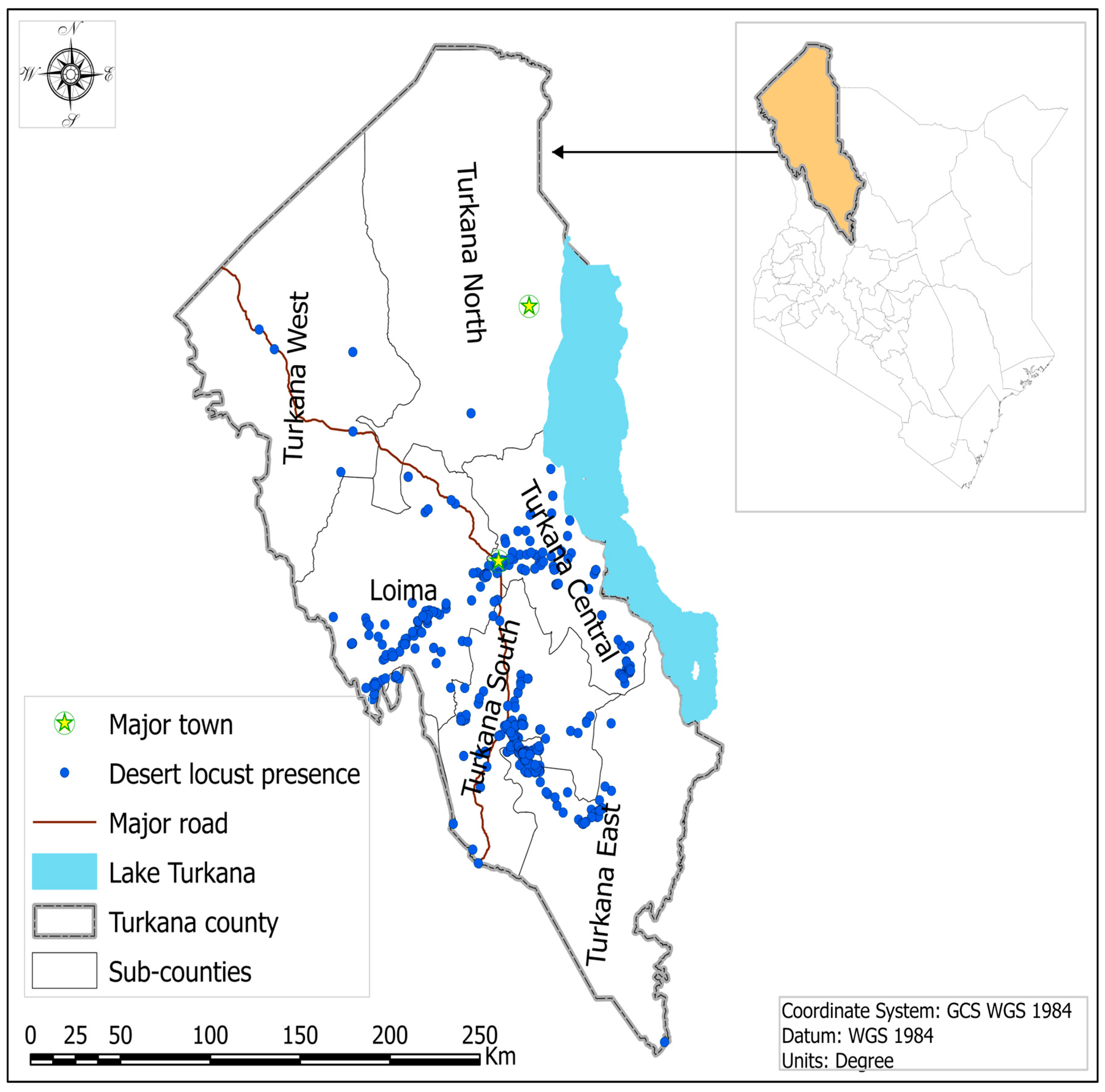
2.1. Study Area
2.2. Data Acquisition and Processing
2.3. Sentinel-2
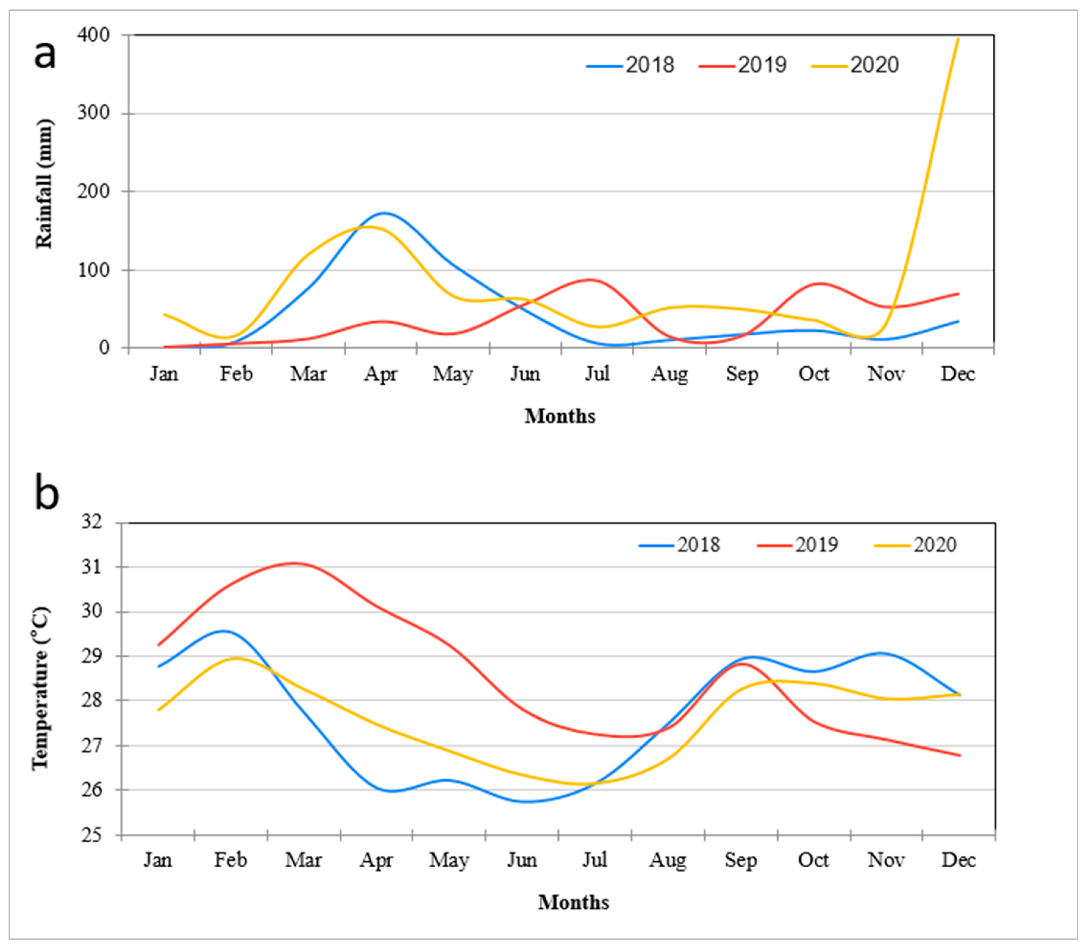
2.4. Daily Climatic Data in the Study Area
2.5. Desert Locust (DL) Occurrence Data
2.6. Bioclimatic Data
2.7. Vegetation Damage Analysis Using the Normalized Difference Vegetation Index (NDVI)
2.8. Current and Future Desert Locust Invasion Risk Analysis
2.9. Ecological Niche Modelling Performance Validation
3. Results
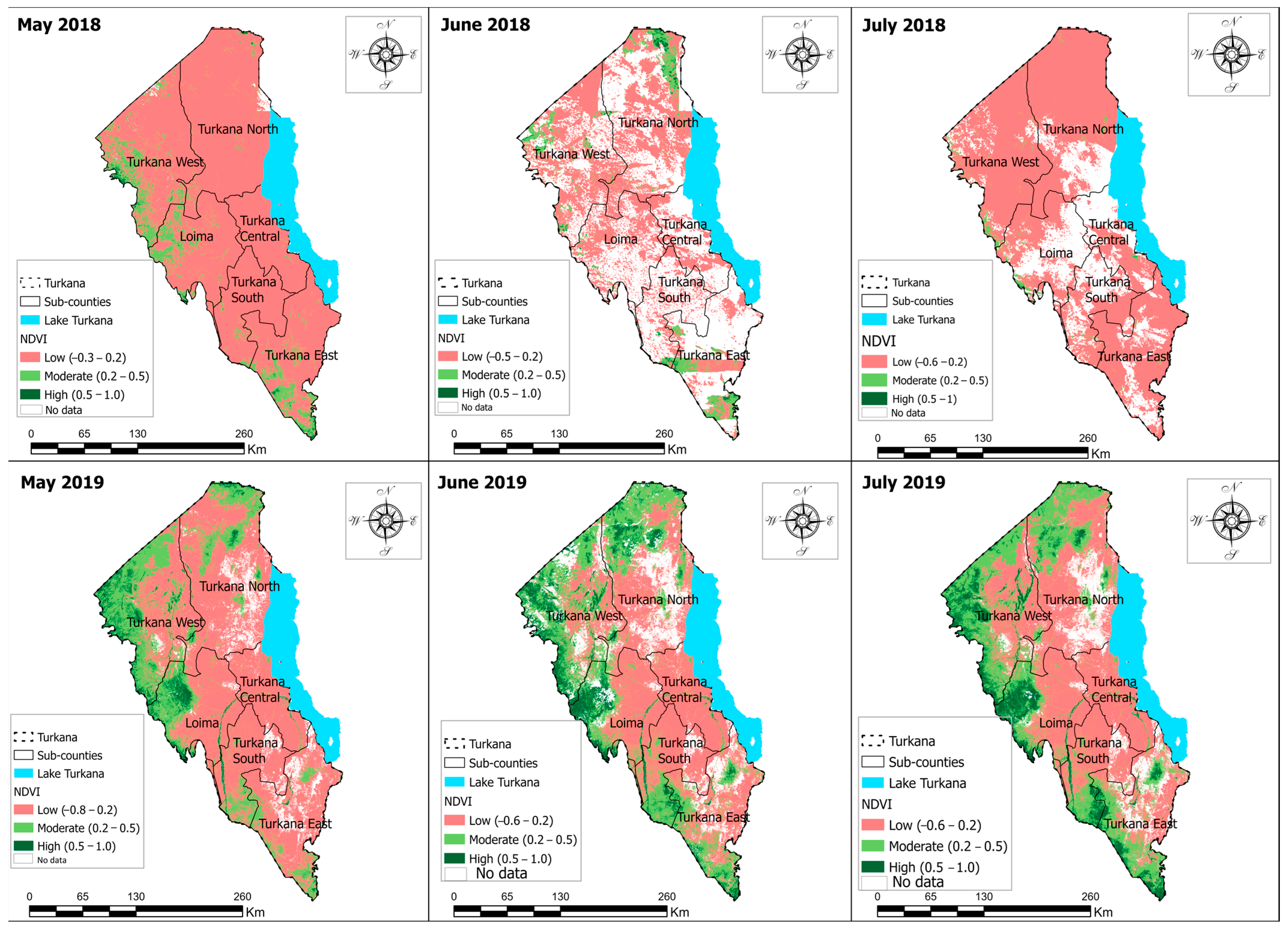
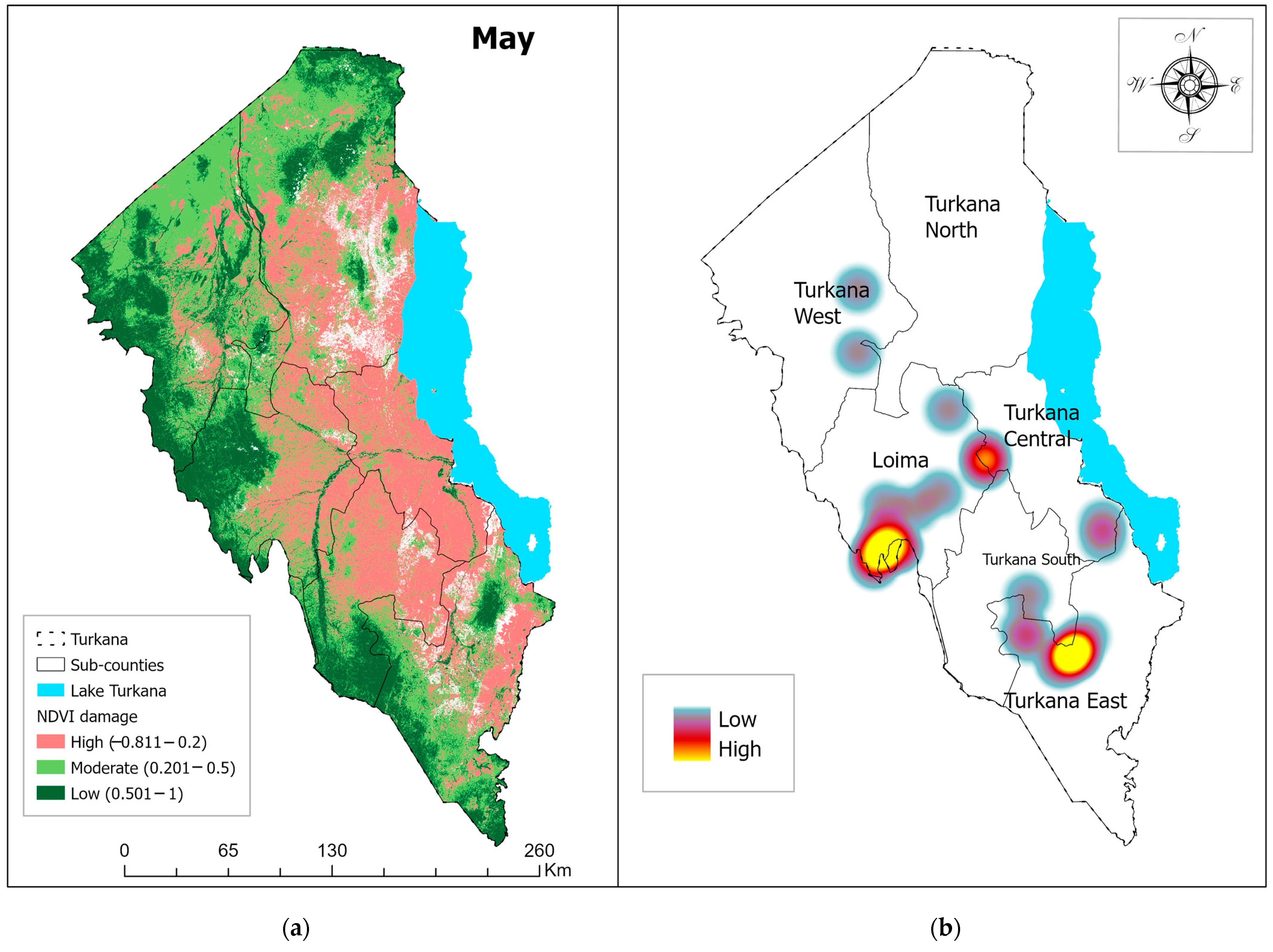
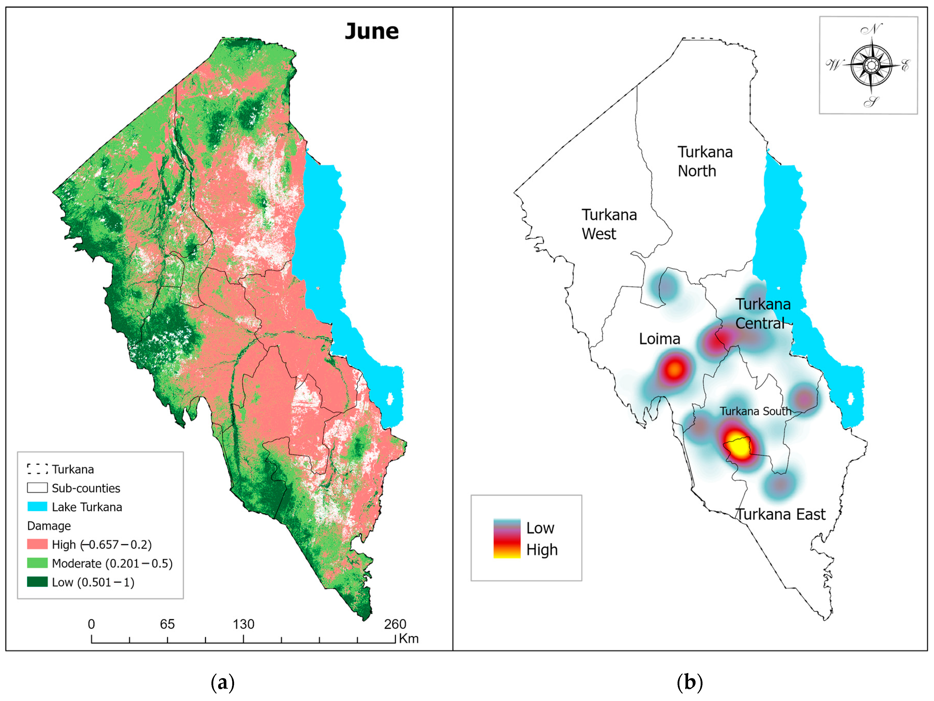
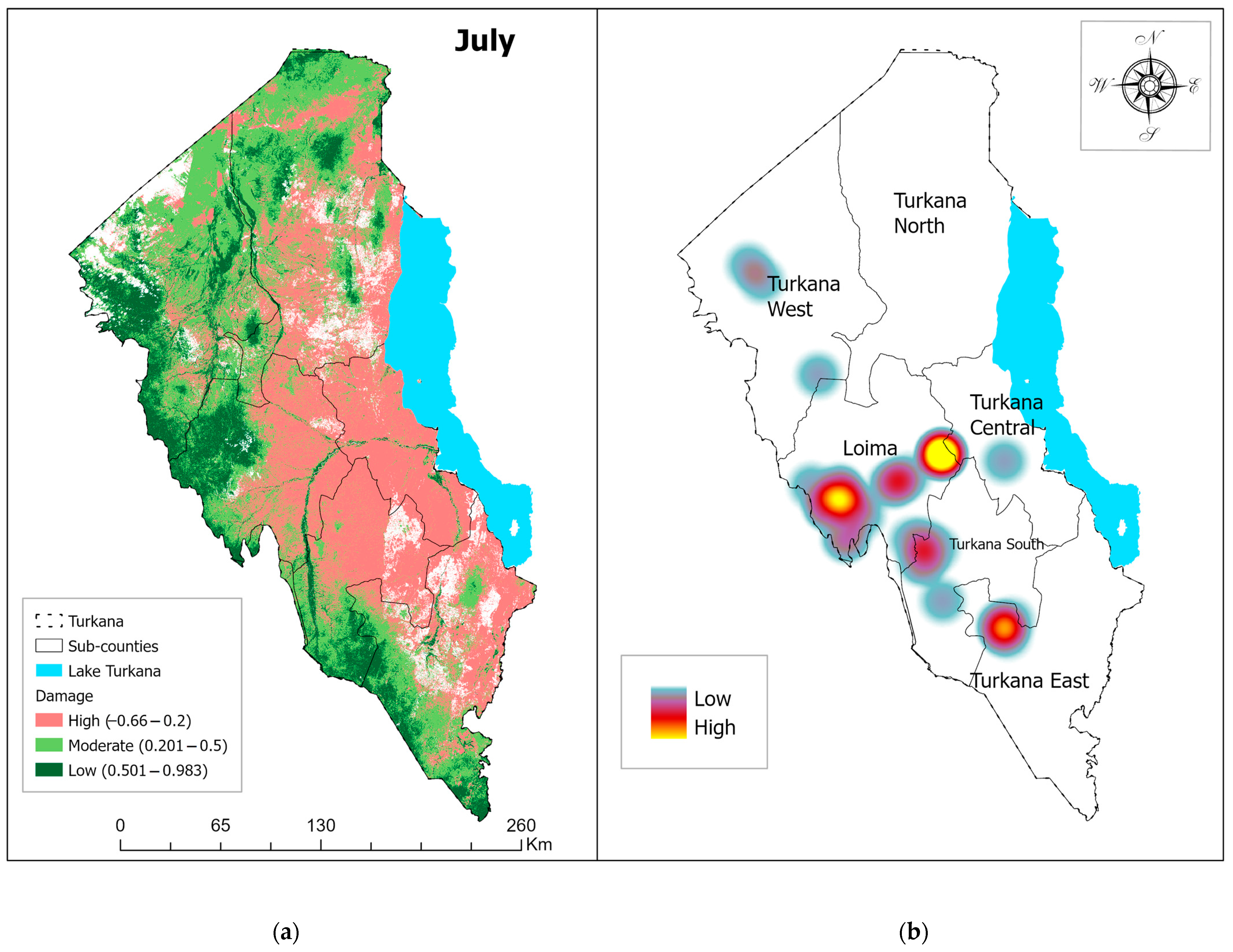
3.1. Vegetation Damage Analysis
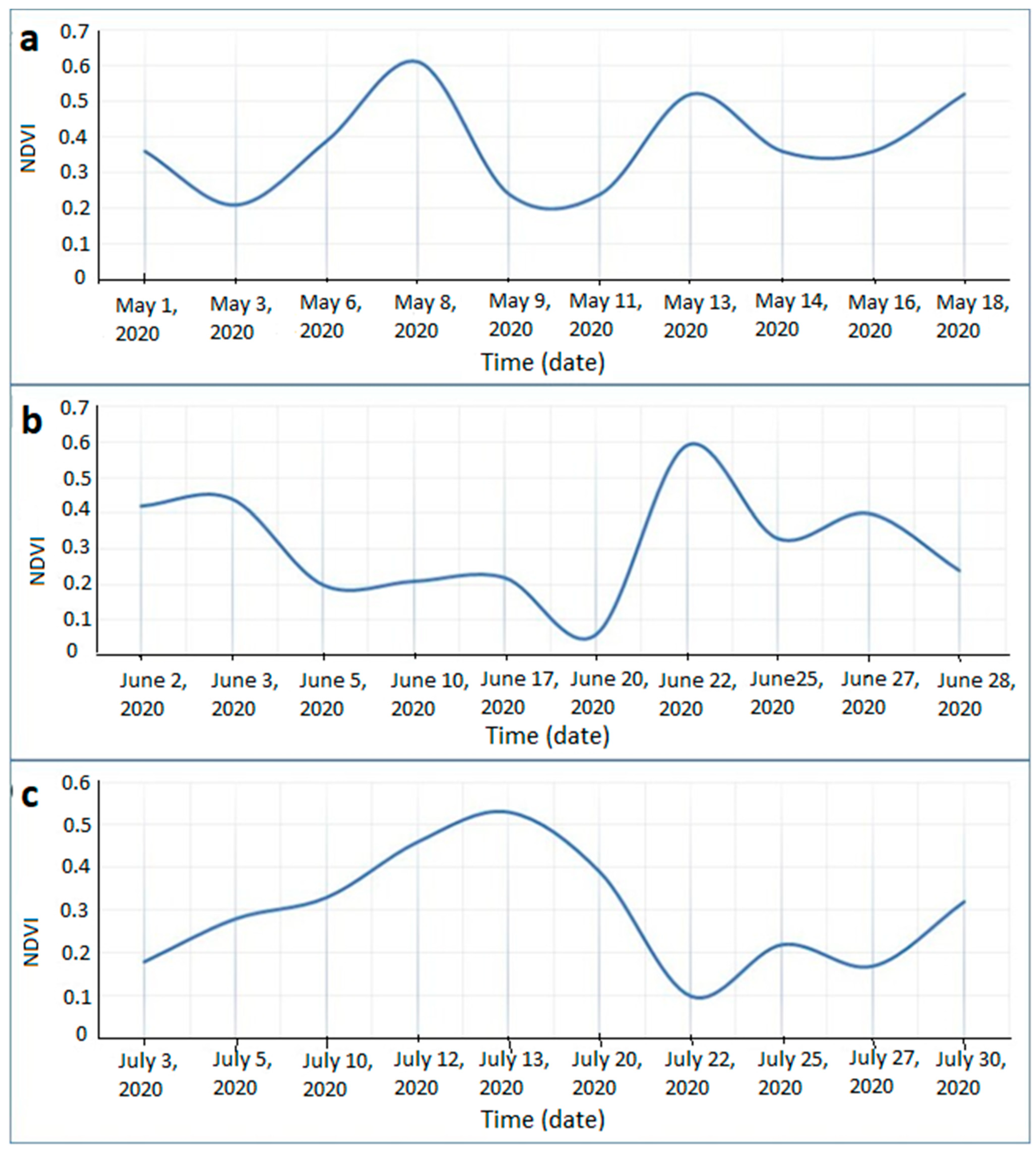
Monthly Normalized Difference Vegetation Index (NDVI) Trend and Vegetation Damage for the Period May–July 2020
3.2. Current and Future Desert Locust Invasion Risk
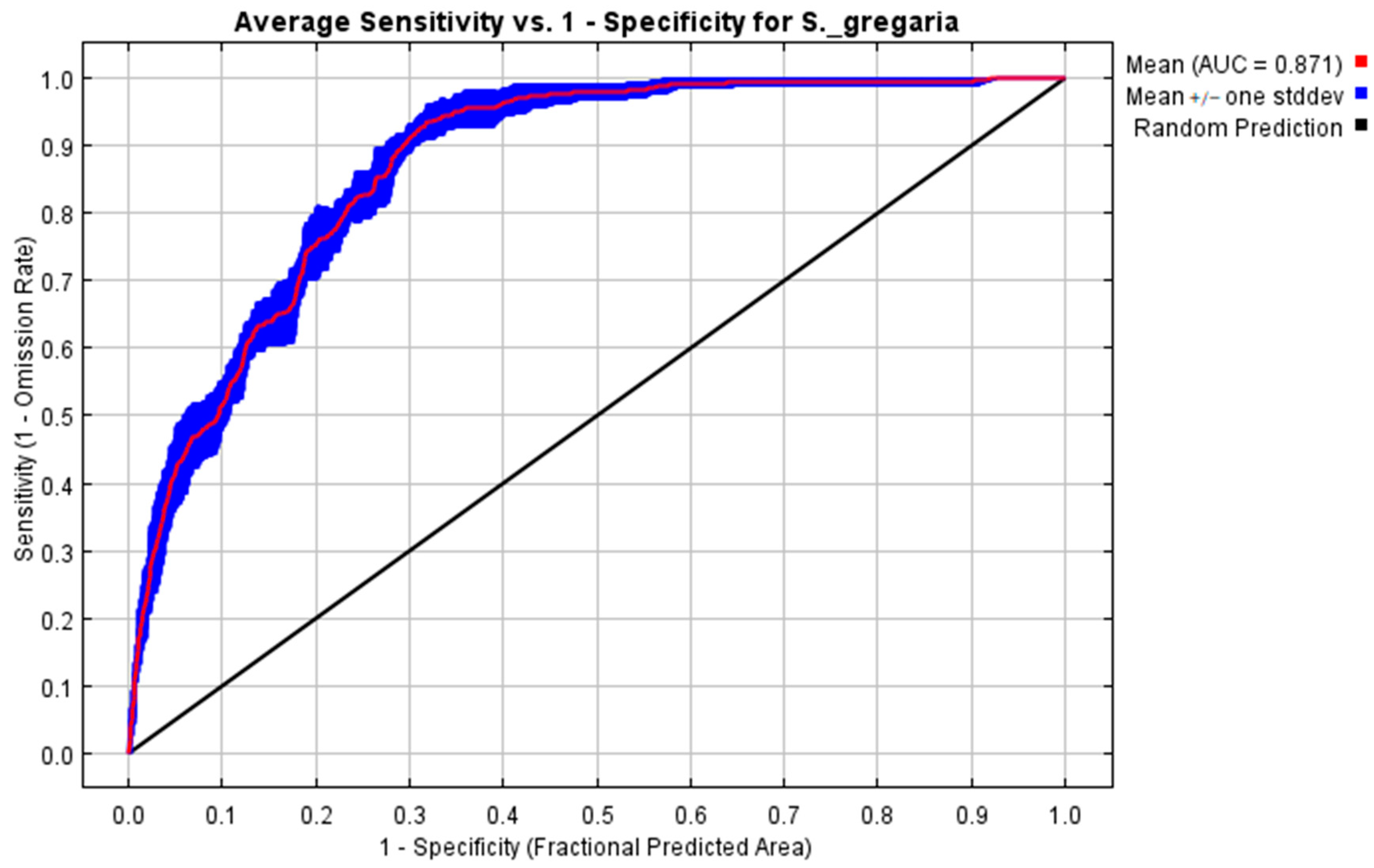
3.2.1. Maximum Entropy (MaxEnt) Model Evaluation
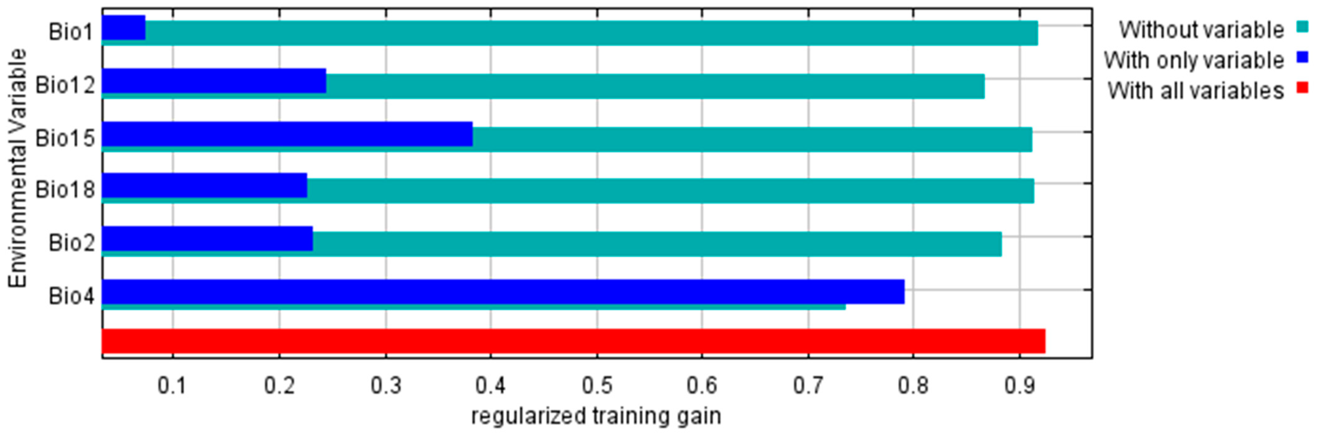
3.2.2. Predictor Variable Contribution on the Maximum Entropy Model
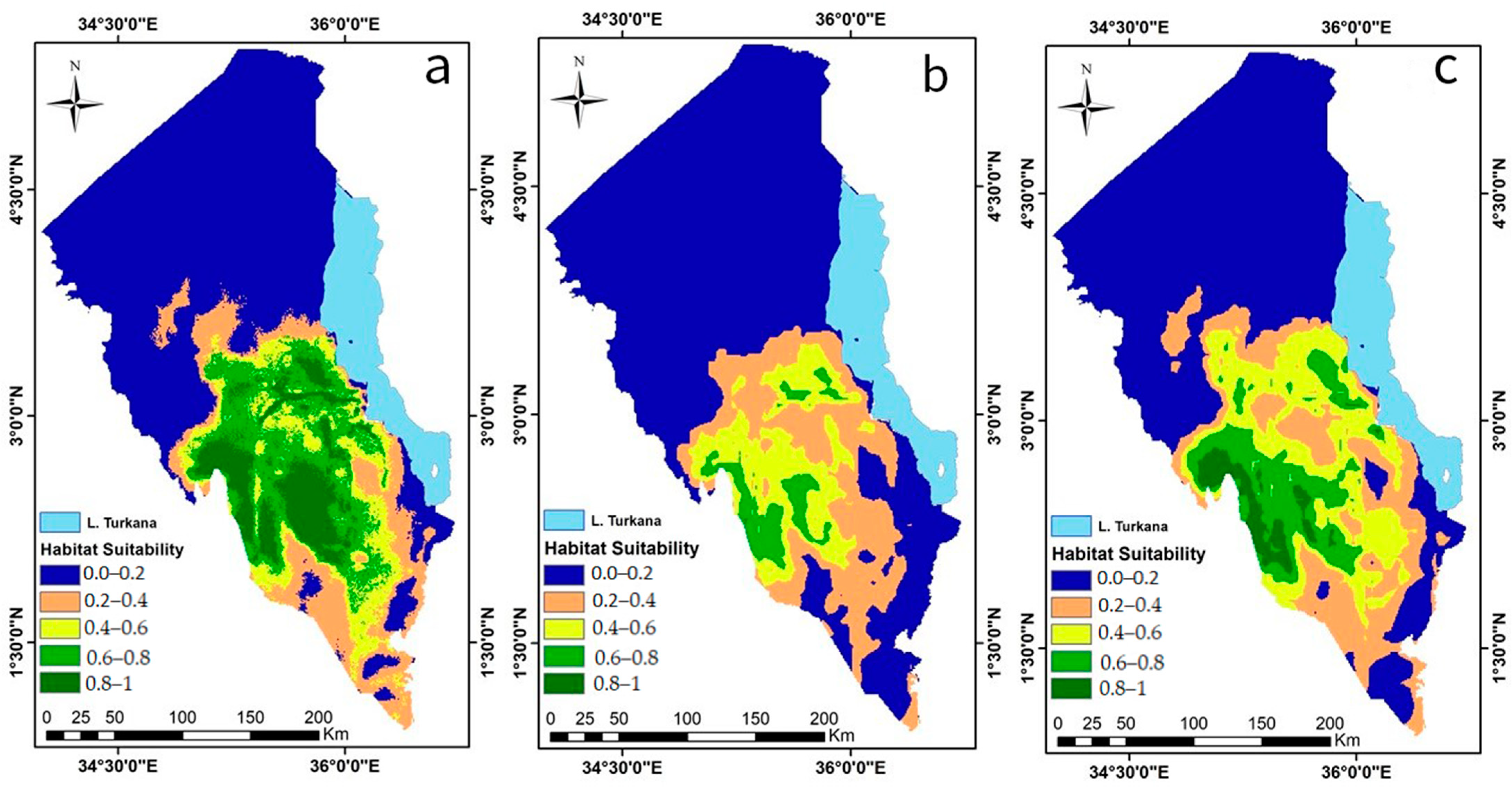
3.2.3. Predicted Current Desert Locust Invasion Risk
3.2.4. Predicted Potential Future Desert Locust Invasion Risk
4. Discussion
4.1. Vegetation Change Analysis
4.2. Predicted Desert Locust Invasion Risk Areas
5. Conclusions
Author Contributions
Funding
Data Availability Statement
Conflicts of Interest
References
- Shrestha, S.; Thakur, G.; Gautam, J.; Acharya, N.; Pandey, M.; Shrestha, J. Desert locust and its management in Nepal: A review. J. Agric. Nat. Resour. 2021, 4, 1–28. [Google Scholar] [CrossRef]
- FAO; WMO. Weather and Desert Locusts. no. 1175. 2016. Available online: https://www.preventionweb.net/publication/weather-and-desert-locust (accessed on 29 January 2021).
- Chen, C.; Qian, J.; Chen, X.; Hu, Z.; Sun, J.; Wei, S.; Xu, K. Geographic distribution of desert locusts in Africa, Asia and Europe using multiple sources of remote-sensing data. Remote Sens. 2020, 12, 3593. [Google Scholar] [CrossRef]
- Waldner, F.; Ebbe, M.A.B.; Cressman, K.; Defourny, P. Operational monitoring of the desert locust habitat with earth observation: An assessment. ISPRS Int. J. Geo-Inf. 2015, 4, 2379–2400. [Google Scholar] [CrossRef] [Green Version]
- Wang, L.; Zhuo, W.; Pei, Z.; Tong, X.; Han, W.; Fang, S. Using long-term earth observation data to reveal the factors contributing to the early 2020 desert locust upsurge and the resulting vegetation loss. Remote Sens. 2021, 13, 680. [Google Scholar] [CrossRef]
- FAO. Desert Locust Bulletin: General Situation During January 2020 Forescast Until Mid-March 2020. 2020, vol. 52420, no. 496. Available online: https://www.fao.org/ag/locusts/common/ecg/562/en/DL496e.pdf (accessed on 15 March 2023).
- FAO. Desert Locust Component: Strengthening Desert Locust Management FAO’s Response to the Desert Locust Problem. 2020. Available online: https://www.fao.org/ag/locusts/common/ecg/1344/en/EMPRESbrochureE.pdf (accessed on 15 March 2023).
- Brader, L.; DJibo, H.; Faya, F.G.; Ghaout, S.; Lazar, M.; Luzietoso, P.N.; Ould-Babah, M.A. Towards a more effective response to desert locusts and their impacts on food security, livelihood and poverty. In Multilateral Evaluation of the 2003–05 Desert Locust Campaign; Food and Agriculture Organisation: Rome, Italy, 2006; pp. 1–42. [Google Scholar]
- Showler, A. Desert locust control: The effectiveness of proactive interventions and the goal of outbreak prevention. Am. Entomol. 2019, 65, 180–191. [Google Scholar] [CrossRef]
- Salih, A.A.M.; Baraibar, M.; Mwangi, K.K.; Artan, G. Climate change and locust outbreak in East Africa. Nat. Clim. Chang. 2020, 10, 584–585. [Google Scholar] [CrossRef]
- Kimathi, E.; Tonnang, H.E.Z.; Subramanian, S.; Cressman, K.; Abdel-Rahman, E.M.; Tesfayohannes, M.; Niassy, S.; Torto, B.; Dubois, T.; Tanga, C.M.; et al. Prediction of breeding regions for the desert locust Schistocerca gregaria in East Africa. Sci. Rep. 2020, 10, 11937. [Google Scholar] [CrossRef]
- FAO. Impact of Desert Locust Infestation on Household Livelihoods and Food Security in Ethiopia. 2020; pp. 1–14. Available online: https://reliefweb.int/report/ethiopia/impact-desert-locust-infestation-household-livelihoods-and-food-security-ethiopia#:~:text=According%20to%20the%20Assessment%20findings,wheat%20at%2036%20000%20hectares (accessed on 27 May 2021).
- Kalakkal, J.; Singh, A. Desert Locusts’ Upsurges: A Harbinger of Emerging Climate Change Induced Crises; The United Nations Environment Programme (UNEP): Nairobi, Kenya, 2021; Volume 22, pp. 1–10. Available online: https://wedocs.unep.org/bitstream/handle/20.500.11822/34226/1/FB019.pdf (accessed on 15 March 2023).
- FAO. Kenya Intensifies Desert Locust Control Measures in Turkana County. 2020. Available online: https://www.fao.org/kenya/news/detail-events/en/c/1279309/#:~:text=Nairobi%2C (accessed on 12 March 2021).
- Eltoum, M. Detection of change in vegetation cover caused by desert locust in Sudan. In Proceedings of the SPIE Asia Pacific Remote Sensing, Beijing, China, 13–16 October 2014. [Google Scholar]
- Cressman, K. Role of remote sensing in desert locust early warning. J. Appl. Remote Sens. 2013, 7, 075098. [Google Scholar] [CrossRef]
- Moustafa, O.R.M.; Cressman, K. Using the enhanced vegetation index for deriving risk maps of desert locust (Schistocerca gregaria, Forskal) breeding areas in Egypt. J. Appl. Remote Sens. 2015, 8, 084897. [Google Scholar] [CrossRef]
- Latchininsky, A.V.; Sivanpillai, R. Locust habitat monitoring and risk assessment using remote sensing and GIS technologies. In Integrated Management of Arthropod Pests and Insect Borne Diseases; Springer: Dordrecht, The Netherlands, 2010. [Google Scholar] [CrossRef]
- Zhu, Y.; Wei, W.; Li, H.; Wang, B.; Yang, X.; Liu, Y. Modelling the potential distribution and shifts of three varieties of Stipa tianschanica in the eastern Eurasian Steppe under multiple climate change scenarios. Glob. Ecol. Conserv. 2018, 16, e00501. [Google Scholar] [CrossRef]
- Li., X.H.; Wang, J.H.; Xing, L.G.; Fu, Y.Y. MaxEnt modelling for predicting climate change effects on the potential planting area of tuber mustard in China. J. Agric. Sci. 2019, 157, 375–381. [Google Scholar] [CrossRef]
- Li, Y.; Li, M.; Li, C.; Liu, Z. Optimized MaxEnt model predictions of climate change impacts on the suitable distribution of Cunninghamia lanceolata in China. Forests 2020, 11, 302. [Google Scholar] [CrossRef] [Green Version]
- Liu, Y.; Shi, J. Predicting the potential global geographical distribution of two Icerya species under climate change. Forests 2020, 11, 684. [Google Scholar] [CrossRef]
- Mudereri, B.T.; Kimathi, E.; Chitata, T.; Moshobane, M.C.; Abdel-Rahman, E.M. Landscape-scale biogeographic distribution analysis of the whitefly, Bemisia tabaci (Gennadius, 1889) in Kenya. Int. J. Trop. Insect Sci. 2021, 41, 1585–1599. [Google Scholar] [CrossRef]
- Garah, K.; Bentouati, A. Using the MaxEnt model for assessing the impact of climate change on the Aurasian Aleppo pine distribution in Algeria. Afr. J. Ecol. 2019, 57, 500–511. [Google Scholar] [CrossRef]
- Mtengwana, B.; Dube, T.; Mudereri, B.T.; Shoko, C. Modelling the geographic spread and proliferation of invasive alien plants (IAPs) into new ecosystems using multi-source data and multiple predictive models in the Heuningnes catchment, South Africa. GIScience Remote Sens. 2021, 58, 483–500. [Google Scholar] [CrossRef]
- Hosni, E.M.; Nasser, M.G.; Al-Ashaal, S.A.; Rady, M.H.; Kenawy, M.A. Modelling current and future global distribution of Chrysomya bezziana under changing climate. Sci. Rep. 2020, 10, 4947. [Google Scholar] [CrossRef] [PubMed] [Green Version]
- Naimi, B.; Araújo, M.B. Sdm: A reproducible and extensible R platform for species distribution modelling. Ecography 2016, 39, 368–375. [Google Scholar] [CrossRef] [Green Version]
- Pearson, R.G.; Raxworthy, C.J.; Nakamura, M.; Townsend, P.A. Predicting species distributions from small numbers of occurrence records: A test case using cryptic geckos in Madagascar. J. Biogeogr. 2007, 34, 102–117. [Google Scholar] [CrossRef]
- Phillips, S.J.; Anderson, R.P.; Schapire, R.E. Maximum entropy modelling of species geographic distributions. Ecol. Modell. 2006, 190, 231–259. [Google Scholar] [CrossRef] [Green Version]
- Paudel, T.B.; Niassy, S.; Kimathi, E.; Abdel-Rahman, E.M.; Seidl-Adams, I.; Wamalwa, M.; Tonnang, H.E.Z.; Ekesi, S.; Hughes, D.P.; Rajotte, E.G.; et al. Potential distribution of fall armyworm in Africa and beyond, considering climate change and irrigation patterns. Sci. Rep. 2022, 12, 539. [Google Scholar] [CrossRef] [PubMed]
- ESA. Sentinel-2 User Handbook, no. 1.2. European Space Agency. 2015. Available online: https://sentinel.esa.int/documents/247904/685211/Sentinel-2_User_Handbook (accessed on 21 June 2021).
- KNBS. Kenya Population and Housing Census Volume 1: Population by County and Sub-County 2019; Volume I. Available online: https://www.knbs.or.ke/?wpdmpro=2019-kenya-population-and-housing-census-volume-i-population-by-county-and-sub-county (accessed on 16 June 2021).
- CIDP. Turkana County Integrated Development Plan (CIDP II) 2018–2022. Available online: https://repository.kippra.or.ke/handle/123456789/2832 (accessed on 21 June 2021).
- Opiyo, F.; Wasonga, O.; Nyangito, M.; Schilling, J.; Munang, R. Drought adaptation and coping strategies among the Turkana pastoralists of northern Kenya. Int. J. Disaster Risk Sci. 2015, 6, 295–309. [Google Scholar] [CrossRef] [Green Version]
- Everlyne, E.; Roxventa, O.; Jackline, K.; Samson, O.; Patrick, M.; Jesse, O. Plant species and their importance to housing in the Turkana community, Kenya. J. Hortic. For. 2020, 12, 101–108. [Google Scholar] [CrossRef]
- Mbaluka, J.K.; Brown, F.H. Vegetation of the Koobi Fora region northeast of Lake Turkana, Marsabit county, northern Kenya. J. East African Nat. Hist. 2016, 105, 21–50. [Google Scholar] [CrossRef]
- Kariuki, J.G.; Machua, J.; Luvanda, A.M.; Kigomo, J.N.; Muindi, F.K.; Macharia, E.W. Baseline Survey of Woodland Utilization and Degradation around Kakuma Refugee Camp (l). Kenya Forestry Research Institute (KEFRI), Nairobi, Kenya. Available online: https://www.fornis.net/sites/default/files/documents/KEFRI%20JOFCA%20Project%20Technical%20Report%20N0.1.pdf (accessed on 21 June 2021).
- Ngigi, W.T. Production of briquettes from Prosopis juliflora stem and anthill soil. Int. J. Nov. Res. Phys. Chem. Math. 2017, 4, 22–27. [Google Scholar]
- Murayama, Y.; Ranagalage, M. Sentinel-2 data for land cover/use mapping: A review. Remote Sens. 2020, 12, 2291. [Google Scholar] [CrossRef]
- Baillarin, S.; Lacherade, S.; Martimort, P.; Agency, E.S.; Spoto, F.; Agency, E.S. Sentinel -2 level 1 products and image processing performances. Int. Arch. Photogramm. Remote Sens. Spatial Inf. Sci. 2012, XXXIX-B1, 197–202. [Google Scholar] [CrossRef] [Green Version]
- Eyring, V.; Bony, S.; Meehl, G.A.; Ronald, S.; Oceanic, N. Overview of the coupled model intercomparison project phase 6 (CMIP6) experimental design and organisation. Geosci. Model Dev. Discuss. 2015, 8, 10539–10583. [Google Scholar] [CrossRef] [Green Version]
- R Core Team. R: A Language and Environment for Statistical Computing. 2021, 2. Available online: https://www.r-project.org/ (accessed on 21 June 2021).
- Wickham, H. Ggplot2: Elegant Graphics for Data Analysis 2016, 35. Available online: http://had.co.nz/ggplot2/book (accessed on 16 October 2021).
- Cressman, K. Desert locust guidelines. 2. Survey,” Food Agric. Organ. United Nations, p. viii + 56pp. 2001. Available online: http://www.fao.org/ag/LOCUSTS/common/ecg/347_en_DLG2e.pdf (accessed on 29 January 2021).
- Fick, S.E.; Hijmans, R.J. WorldClim 2: New 1-km spatial resolution climate surfaces for global land areas. Int. J. Climatol. 2017, 37, 4302–4315. [Google Scholar] [CrossRef]
- Tatebe, H.; Ogura, T.; Nitta, T.; Komuro, Y.; Ogochi, K.; Takemura, T.; Sudo, K.; Sekiguchi, M.; Abe, M.; Saito, F.; et al. Description and basic evaluation of simulated mean state, internal variability, and climate sensitivity in MIROC6. Geosci. Model Dev. 2018, 12, 2727–2765. [Google Scholar] [CrossRef] [Green Version]
- Hijmans, R.J.; Etten, J.V.; Sumner, M.; Cheng, J.; Baston, D.; Bevan, A.; Bivand, R.; Busetto, L.; Canty, M.; Fasoli, B.; et al. Raster: Geographic Data Analysis and Modelling. R package version 3.3–7. 2020. Available online: https://cran.r-project.org/package=raster (accessed on 21 June 2021).
- Roy, D.P.; Li, J.; Zhang, H.K.; Yan, L. Best practices for the reprojection and resampling of sentinel-2 multi spectral instrument level 1c data. Remote Sens. Lett. 2016, 7, 1023–1032. [Google Scholar] [CrossRef] [Green Version]
- Leroy, M.B.; Meynard , C.N.; Bellard , C.; Courchamp , F. Virtualspecies, an R package to generate virtual species distributions. Ecography 2015. [Google Scholar] [CrossRef] [Green Version]
- IPCC. Assessment Report 6 Climate Change 2021: The Physical Science Basis. 2021. Available online: https://www.ipcc.ch/report/ar6/wg1/ (accessed on 15 November 2021).
- Meinshausen, M.; Nicholls, Z.; Lewis, J.; Gidden, M.; Vogel, E.; Freund, M.; Beyerle, U.; Gessner, C.; Nauels, A.; Bauer, N.; et al. The SSP greenhouse gas concentrations and their extensions to 2500. Geosci. Model Dev. Discuss. 2019, 13, 3571–3605. [Google Scholar] [CrossRef]
- Ali, S.M.; Jassem, D.R. Monitoring vegetation areas by using remote sensing techniques. Int. J. Comp. Info. Tech. 2015, 3, 1–9. [Google Scholar] [CrossRef]
- Neigh, C.S.R.; Tucker, C.J.; Townshend, J.R.G. North American vegetation dynamics observed with multi-resolution satellite data. Remote Sens Env. 2008, 112, 1749–1772. [Google Scholar] [CrossRef] [Green Version]
- Pettorelli, N.; Ryan, S.; Mueller, T.; Bunnefeld, N. The normalized difference vegetation index (NDVI): Unforeseen successes in animal ecology. Clim. Res. 2011, 46, 15–27. [Google Scholar] [CrossRef]
- Schmid, J.N. Using Google Earth Engine for Landsat NDVI Time Series Analysis to Indicate the Present Status of Forest Stands. Bachelor’s Thesis, Georg-August-Universität Göttingen, Göttingen, Germany, October 2017. [Google Scholar] [CrossRef]
- Mutanga, O.; Kumar, L. Google Earth Engine applications. Remote Sens. 2019, 11, 591. [Google Scholar] [CrossRef] [Green Version]
- Sivarajah, M. An Introduction to Google Earth Engine javascript API. 2019, 416–424. Available online: https://earthengine.google.com/%0Ahttps://sovzond.ru/press-center/news/corporate/6095/ (accessed on 28 June 2021).
- Bey, A.; Jetimane, J.; Lisboa, S.N.; Ribeiro, N.; Sitoe, A.; Meyfroidt, P. Mapping smallholder and large-scale cropland dynamics with a flexible classification system and pixel-based composites in an emerging frontier of Mozambique. Remote Sens. Environ. 2020, 239, 111611. [Google Scholar] [CrossRef]
- Hashim, H.; Abd-Latif, Z.; Adnan, N.A. Urban vegetation classification with NDVI threshold value method with very high resolution (VHR) Pleiades imagery. Int. Arch. Photogramm. Remote Sens. Spat. Inf. Sci. 2019, 42, 237–240. [Google Scholar] [CrossRef] [Green Version]
- Baloch, M.N.; Fan, J.; Haseeb, M.; Zhang, R. Mapping potential distribution of Spodoptera frugiperda (Lepidoptera: Noctuidae) in Central Asia. Insects 2020, 11, 172. [Google Scholar] [CrossRef] [Green Version]
- Elith, J.; Phillips, S.J.; Hastie, T.; Dudík, M.; Chee, Y.E.; Yates, C.J. A statistical explanation of MaxEnt for ecologists. Divers. Distrib. 2011, 17, 43–57. [Google Scholar] [CrossRef]
- Phillips, S.J. A Brief Tutorial on MaxEnt. AT&T Res. 2018, 190, 231–259. [Google Scholar]
- Muscarella, R.; Galante, P.J.; Soley-guardia, M.; Boria, R.A.; Kass, J.M.; Anderson, R.P. ENMeval: An R package for conducting spatially independent evaluations and estimating optimal model complexity for maxent ecological niche models. Methods Ecol. Evol. 2014, 5, 1198–1205. [Google Scholar] [CrossRef] [Green Version]
- Arthur, F.H.; Iii, W.R.M.; Morey, A.C. Modelling the potential range expansion of larger grain borer, Prostephanus truncatus (Coleoptera: Bostrichidae). Sci. Rep. 2018, 9, 6862. [Google Scholar] [CrossRef] [PubMed] [Green Version]
- Qin, A.; Liu, B.; Guo, Q.; Bussmann, R.W.; Ma, F.; Jian, Z.; Xu, G.; Pei, S. MaxEnt modelling for predicting impacts of climate change on the potential distribution of Thuja sutchuenensis Franch., an extremely endangered conifer from southwestern China. Glob. Ecol. Conserv. 2017, 10, 139–146. [Google Scholar] [CrossRef]
- Merow, C.; Smith, M.J.; Silander, J.A. A practical guide to MaxEnt for modelling species’ distributions: What it does, and why inputs and settings matter. Ecography 2013, 36, 1058–1069. [Google Scholar] [CrossRef]
- Adan, M.; Abdel-Rahman, E.M.; Gachoki, S.; Muriithi, B.W.; Lattorff, H.M.G.; Kerubo, V.; Landmann, T.; Mohamed, S.A.; Tonnang, H.E.Z.; Dubois, T. Use of earth observation satellite data to guide the implementation of integrated pest and pollinator management (IPPM) technologies in an avocado production system. Remote Sens. Appl. Soc. Environ. 2021, 23, 100566. [Google Scholar] [CrossRef]
- Roberts, D.; Mueller, N.; McIntyre, A. High-dimensional pixel composites from earth observation time series. IEEE Trans. Geosci. Remote Sens. 2017, 55, 6254–6264. [Google Scholar] [CrossRef]
- NDMA. Turkana County Drought Early Warning Bulletin for July 2020; National Drought Management Authority: Nairobi, Kenya, 2020; pp. 1–14.
- WMO. Heavy rains contribute to desert locust crisis in East Africa. 2020. Available online: https://public.wmo.int/en/media/news/heavy-rains-contribute-desert-locust-crisis-east-africa (accessed on 13 July 2021).
- Zhang, W.; Brandt, M.; Tong, X.; Tian, Q.; Fensholt, R. Impacts of the seasonal distribution of rainfall on vegetation productivity across the Sahel. Biogeosciences 2018, 15, 319–330. [Google Scholar] [CrossRef] [Green Version]
- Mohamed, N.; Bannari, A. The relationship between vegetation and rainfall in central Sudan. Int. J. Remote Sens. Appl. 2016, 6, 30. [Google Scholar] [CrossRef]
- Turkana County Government. Turkana County climate Change Policy 2020 Draft 1. 2020. Available online: https://www.turkana.go.ke/wp-content/uploads/2020/09/Book.pdf (accessed on 13 July 2021).
- Yang, X.Q.; Kushwaha, S.P.S.; Saran, S.; Xu, J.; Roy, P.S. MaxEnt modelling for predicting the potential distribution of medicinal plant, Justicia adhatoda L. in Lesser Himalayan foothills. Ecol. Eng. 2013, 51, 83–87. [Google Scholar] [CrossRef]
- Çoban, H.O.; Örücü, Ö.K.; Arslan, E.S. MaxEnt modelling for predicting the current and future potential geographical distribution of Quercus libani olivier. Sustainability 2020, 12, 2671. [Google Scholar] [CrossRef] [Green Version]
- Nayak, S.B.; Rao, K.S.; Ramalakshmi, V. Impact of climate change on insect pests and their natural enemies Sudhanshu. Int. J. Ecol. Environ. Sci. 2020, 2, 579–584. [Google Scholar]
- Skendžić, S.; Zovko, M.; Živković, I.P.; Lešić, V.; Lemić, D. The impact of climate change on agricultural insect pests. Insects 2021, 12, 440. [Google Scholar] [CrossRef]
- Symmons, P.M.; Cressman, K. Desert Locust Guidelines, Biology and behaviour, 2nd ed.; Food and Agriculture Organization, United Nations: Rome, Italy, 2001; p. 42. [Google Scholar]
- Borzée, A.; Andersen, D.; Groffen, J.; Kim, H.T.; Bae, Y.; Jang, Y. Climate change-based models predict range shifts in the distribution of the only Asian plethodontid salamander: Karsenia koreana. Sci. Rep. 2019, 9, 11838. [Google Scholar] [CrossRef] [Green Version]
- Olang, M.O. Vegetation Cover Assessment in Turkana District, Kenya; International Institute for Land Reclamation and Improvement: Wageningen, The Netherlands, 1983; pp. 183–193. [Google Scholar]
- Garrido, R.; Bacigalupo, A.; Peña-Gómez, F.; Bustamante, R.O.; Cattan, P.E.; Gorla, D.E.; Botto-Mahan, C. Potential impact of climate change on the geographical distribution of two wild vectors of Chagas disease in Chile: Mepraia spinolai and Mepraia gajardoi. Parasites Vectors 2019, 12, 478. [Google Scholar] [CrossRef] [PubMed]
- Gandhi, G.M.; Parthiban, S.; Thummalu, N.; Christy, A. Ndvi: Vegetation change detection using remote sensing and GIS—A case study of Vellore district. Procedia Comput. Sci. 2015, 57, 1199–1210. [Google Scholar] [CrossRef] [Green Version]
- Oikonomopoulos, E. NDVI Time Series Analysis for Desert Locust Outbreak Detection and Quantification Analysis of Its Impact on Vegetation Productivity of Sahel. Master’s Thesis, Lund University, Lund, Sweden, 2020. [Google Scholar]


| Band | Band Description | Central Wavelength (nm) | Pixel Size (m) |
|---|---|---|---|
| B1 | Coastal aerosol | 443 | 60 |
| B2 | Blue | 490 | 10 |
| B3 | Green | 560 | 10 |
| B4 | Red | 665 | 10 |
| B5 | Red-edge 1 (RE1) | 705 | 20 |
| B6 | Red-edge 2 (RE2) | 740 | 20 |
| B7 | Red-edge 3 (RE3) | 783 | 20 |
| B8 | Near-infrared (NIR) | 842 | 10 |
| B8a | Narrow NIR (NNIR) | 865 | 20 |
| B9 | Short wave infrared (SWIR1)-water vapor | 940 | 60 |
| B10 | Short wave infrared (SWIR2)-cirrus | 1375 | 60 |
| B11 | Short wave infrared (SWIR3) | 1610 | 20 |
| B12 | Short wave infrared (SWIR4) | 2190 | 20 |
| Bioclimate Code | Variable Description | Unit |
|---|---|---|
| Bio1 | Annual mean temperature | °C |
| Bio2 | Mean diurnal range | °C |
| Bio3 | Isothermality | NU * |
| Bio4 | Temperature seasonality | NU * |
| Bio5 | Max temperature of warmest month | °C |
| Bio6 | Min temperature of coldest month | °C |
| Bio7 | Temperature annual range | °C |
| Bio8 | Mean temperature of wettest quarter | °C |
| Bio9 | Mean temperature of driest quarter | °C |
| Bio10 | Mean temperature of warmest quarter | °C |
| Bio11 | Mean temperature of coldest quarter | °C |
| Bio12 | Annual precipitation | mm |
| Bio13 | Precipitation of the wettest month | mm |
| Bio14 | Precipitation of the driest month | mm |
| Bio15 | Precipitation seasonality | NU * |
| Bio16 | Precipitation of the wettest quarter | mm |
| Bio17 | Precipitation of the driest quarter | mm |
| Bio18 | Precipitation of the warmest quarter | mm |
| Bio19 | Precipitation of coldest quarter | mm |
| Bioclimate Code | Variable Description | Contribution (%) |
|---|---|---|
| Bio4 | Temperature seasonality | 83.1 |
| Bio2 | Mean diurnal range | 4.8 |
| Bio18 | Precipitation of the warmest quarter | 4.0 |
| Bio12 | Annual precipitation | 3.9 |
| Bio15 | Precipitation seasonality | 2.4 |
| Bio1 | Annual mean temperature | 1.7 |
| Period | Climate Scenario (MIROC 6 Climate Model) | Area (km2) | Percentage of the Total Area |
|---|---|---|---|
| Current | 18937.67 | 27.15 | |
| 2030 | SSP2-4.5 | 6455.62 | 9.25 |
| SSP5-8.5 | 14192.74 | 20.34 |
Disclaimer/Publisher’s Note: The statements, opinions and data contained in all publications are solely those of the individual author(s) and contributor(s) and not of MDPI and/or the editor(s). MDPI and/or the editor(s) disclaim responsibility for any injury to people or property resulting from any ideas, methods, instructions or products referred to in the content. |
© 2023 by the authors. Licensee MDPI, Basel, Switzerland. This article is an open access article distributed under the terms and conditions of the Creative Commons Attribution (CC BY) license (https://creativecommons.org/licenses/by/4.0/).
Share and Cite
Mongare, R.; Abdel-Rahman, E.M.; Mudereri, B.T.; Kimathi, E.; Onywere, S.; Tonnang, H.E.Z. Desert Locust (Schistocerca gregaria) Invasion Risk and Vegetation Damage in a Key Upsurge Area. Earth 2023, 4, 187-208. https://doi.org/10.3390/earth4020010
Mongare R, Abdel-Rahman EM, Mudereri BT, Kimathi E, Onywere S, Tonnang HEZ. Desert Locust (Schistocerca gregaria) Invasion Risk and Vegetation Damage in a Key Upsurge Area. Earth. 2023; 4(2):187-208. https://doi.org/10.3390/earth4020010
Chicago/Turabian StyleMongare, Raphael, Elfatih M. Abdel-Rahman, Bester Tawona Mudereri, Emily Kimathi, Simon Onywere, and Henri E. Z. Tonnang. 2023. "Desert Locust (Schistocerca gregaria) Invasion Risk and Vegetation Damage in a Key Upsurge Area" Earth 4, no. 2: 187-208. https://doi.org/10.3390/earth4020010