
Multiscale Correlation Analysis between Wind Direction and Meteorological Parameters in Guadeloupe Archipelago


1
Department of Research in Geoscience, KaruSphère SASU, Guadeloupe (F.W.I.), 97139 Abymes, France
2
LaRGE Laboratoire de Recherche en Géosciences et Energies (EA 4935), University of the Antilles, 97100 Pointe-à-Pitre, France
3
TKM College of Engineering Kollam, Kerala 691005, India
*
Author to whom correspondence should be addressed.
Earth 2023, 4(1), 151-167; https://doi.org/10.3390/earth4010008
Submission received: 30 January 2023
/
Revised: 23 February 2023
/
Accepted: 27 February 2023
/
Published: 10 March 2023
Abstract
:In this paper, the wind direction () behaviour with respect to the variability of other meteorological parameters (i.e., rainfall (R), temperature (T), relative humidity (), solar radiation () and wind speed (U)) was studied in a multi-scale way. To carry out this study, the Hilbert–Huang transform (HHT) framework was applied to a Guadeloupe archipelago dataset from 2016 to 2021. Thus, the time-dependent intrinsic correlation (TDIC) analysis based on multivariate empirical mode decomposition (MEMD) was performed. For time scales between ∼3 days and ∼7 months, the localized positive and negative correlations between and the meteorological parameters have been identified. The alternation between these correlations was more significant for T and . With regard to and U, there was a dominance of a negative correlation with . We assumed that the micro-climate previously identified in the literature for the study area plays a key role in these behaviours. A strong positive correlation between and R was found from ∼7 months to ∼2.5 years. At the annual scale, the relationships between and all meteorological parameters were long range and no significant transition in correlation was observed showing the impact of the Earth’s annual cycle on climatic variables. All these results clearly show the influence of R-T---U on over different time scales.
1. Introduction
Nowadays, waste management is a worldwide societal issue [1,2,3,4]. In insular contexts, waste management is a main problem due to the lack of space. Open landfills are often located in the heart of agglomerations [5,6]. Apart from the nauseating odours emitted by these storage centres, the atmospheric pollutants emitted by this municipal solid waste may have a significant health impact on the neighbouring populations [7,8,9]. In a place where there are many micro-climates, it is crucial to better understand the fate of these pollutants.
In the literature, it is well known that meteorological parameters play an important role in pollutant dilution, diffusion, advection and transformation [10,11,12]. The wind is a preponderant climatic variable in these processes. Studies on wind speed behaviour are highly significant, because strong winds allow the dispersion of air pollutants in the atmospheric boundary layer, while calm winds promote its stagnation [13,14,15,16,17,18]. Nevertheless, wind direction is also a key feature as it determines the path of pollutants. In the air pollution field, the behaviour of wind direction is usually studied using statistical methods [19,20,21,22,23,24]. Although these studies provide information on the statistical behaviour of this parameter, its dynamics are not taken into account. Indeed, the results of these works are based only on a single time scale and might not necessarily reflect the features of wind direction time series over several scales [25,26]. To our knowledge, no study has yet investigated the relationship between wind direction and other meteorological parameters using the Hilbert–Huang transform (HHT) framework. For the first time, the coupled multivariate empirical mode decomposition (MEMD) [27] and time-dependent intrinsic correlation (TDIC) framework [28] are used to analyse the teleconnection between wind direction and rainfall, temperature, relative humidity, solar radiation and wind speed. The aim of this study was to analyse wind direction behaviour according to the aforementioned meteorological parameters over several time scales.
2. Materials and Methods
2.1. Study Area and Data Description
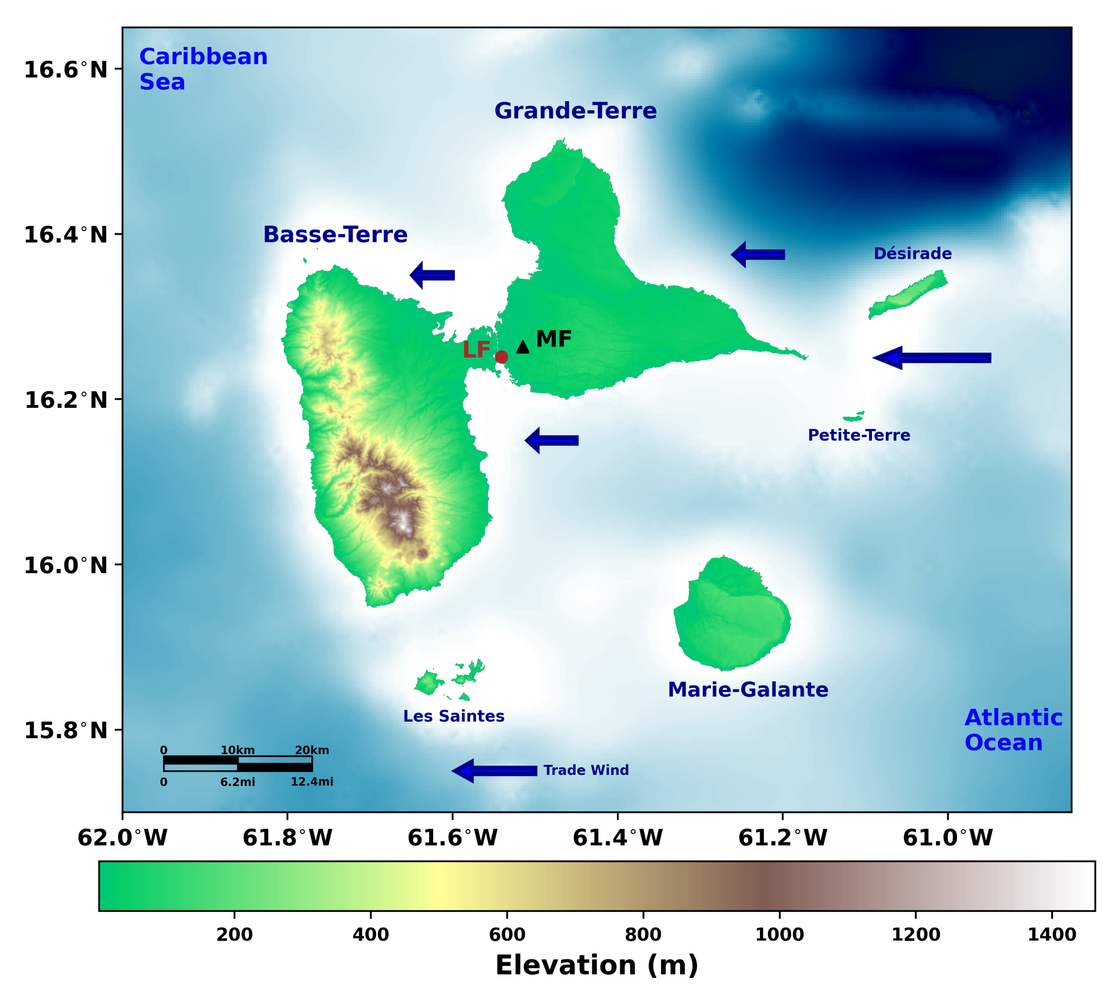
The Guadeloupe archipelago (16.25° N–61.58° W) is a French West Indies island located in the middle of the Lesser Antilles in the Caribbean basin. With an area of ∼1800 km2 and a population of 390,250 inhabitants [29], this island experiences a tropical rainforest climate (“Af”) according to the Köppen–Geiger classification [30]. The study area is in the centre of Guadeloupe (Figure 1) where the topography is nearly flat and concrete buildings do not exceed four floors. The main open landfill of the island ( in Figure 1) is in the same location [31]. Embedded in a mangrove area that surrounds it, the is sandwiched between the mangrove and a densely urbanized area [5,6]. This area is the most populated area of Guadeloupe [15].
The meteorological measurements (i.e., rainfall (R), temperature (T), relative humidity (), solar radiation (), wind speed (U) and wind direction ()) were carried out by Météo France (https://meteofrance.gp/fr, 30 January 2023, in Figure 1) in the study area on the international airport of Les Abymes (16.2630° N –61.61.5147° W). In order to study the relationship between and the other meteorological parameters, a daily database was available from 2016 to 2021, i.e., 1827 points per time series. To guarantee the validity of the data, the latter were previously pre-processed by . In Figure 1, we can observe that and are close. Classically, the prevailing wind in the Caribbean basin comes from the east (∼90), i.e., the trade wind. As exhibits huge fluctuations over time due to many factors such as topography [32], the predominant of each day was used in our analysis for a better understanding of its multi-scale behaviour.
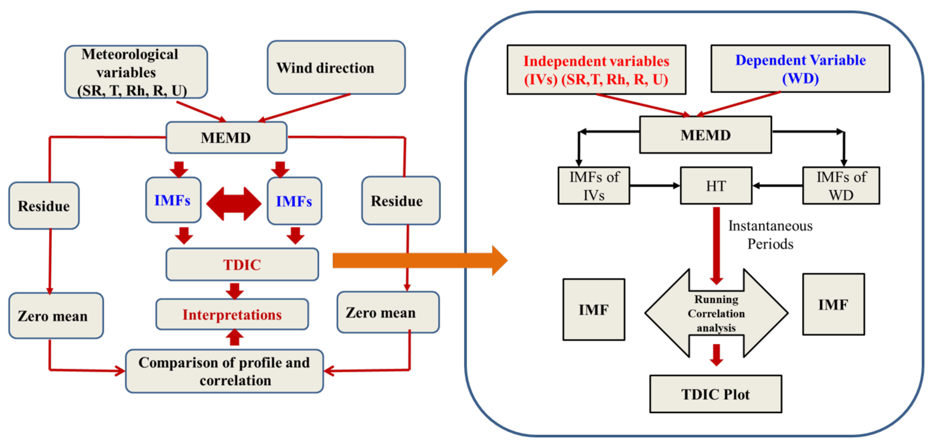
2.2. Multi-Scale Multidimensional Correlation Analysis
2.2.1. MEMD
Within 25 years of its introduction, HHT has gained wide popularity for the spectral analysis of non-linear and non-stationary time series data [33]. It is a purely data adaptive method, which can produce physically meaningful representations of time series data. This method does not require a priori selection of functions, but instead it decomposes the signal into intrinsic oscillation modes derived from the succession of extrema. The HHT involves two major steps (i), the use of the empirical mode decomposition (EMD) method or its variants, such as the ensemble EMD (EEMD), or the complete EEMD with adaptive noise (CEEMDAN) [34,35], to decompose a time series into a collection of orthogonal time series, namely, intrinsic mode functions (IMFs), and a final residue; (ii) the use of Hilbert spectral analysis (HSA) to obtain the instantaneous frequency which may be helpful to identify embedded structures of the time series data.
The EMD method decomposes a time series into a set of zero mean components and a final residue, each with specific periodicity. The decomposition is carried out based on the physical time scales that characterize the oscillations of the phenomena [36]. Different non-stationary oscillation processes controlling the variables are governed by the IMFs of the EMD [37]. In a broad sense, comparing the periodicity of the modes with that of the driving factors governs the basis of teleconnection studies [38,39]. For such studies on geophysical time series, the meteorological factors or large-scale climatic oscillations are often considered as predictors. The residue shows the long-term inherent trend of the time series and a comparison between the residue components of the variables and governing factors are likely to be well correlated [40]. The trend is an intrinsically fitted monotonic function or a function in which there can be at most one extremum within a given data span [41]. In this study, the trend represents the changes or alternations in the most likely magnitude of the wind direction throughout time.
The EMD or its variants work well for single time series data at a time and it may result in a different number of data modes adaptively, based on data complexity. This may impose difficulties in developing hybrid decomposition models [42,43] and a decomposition method, which can result in an equal number of modes being a viable option in multi-scale correlation studies, especially when multiple time series are involved. Multivariate EMD, proposed by Rehman and Mandic [27], is an extension of the traditional EMD, which decomposes multiple time series simultaneously after identifying the common scales inherent in different time series of concern. In this method, multiple envelopes are produced by taking projections of multiple inputs along different directions in an m-dimensional space.
Assuming being the m vectors as a function of time t, and denoting the direction vector along different directions given by angles in a direction set X (, where K is the total number of directions). It can be noted that the rotational modes appear as the counterparts of the oscillatory modes in EMD or its variants. The IMFs of m temporal datasets can be obtained by the following steps:
- 1.
- A suitable set of direction vectors are generated by sampling on a unit hyper-sphere;
- 2.
- The projection of the dataset are calculated along the direction vector for all k;
- 3.
- Temporal instants are identified corresponding to the maxima of projection for all k;
- 4.
- is interpolated to obtain multivariate envelope curves for all k;
- 5.
- The mean of envelope curves is calculated by ;
- 6.
- The “detail” is extracted using . If fulfils the stoppage criterion for a multivariate IMF, the above procedure from step (1) onwards is applied upon the residue series (i.e., ). Otherwise, steps from (2) onwards are repeated upon the series .
The Hammersley sampling sequence can be used for the generation of direction vectors [44] and the stoppage criteria proposed for the EMD (i.e., the sum squared difference between the deviations of the mode from the mean signal in two consecutive iterations should be less than a specified tolerance) can be used in the implementation of the MEMD.
2.2.2. HSA
In the HSA, firstly the is convoluted with the function to obtain HT. As the function is a non-integrable one, the Cauchy principal value (PV) is considered instead of finding HT, in the following form [45]:
Hence, any signal can be represented by combining and its HT as follows:
where , is the amplitude, and is the phase angle, which are defined as:
In HSA, the amplitude and phase angle are both functions of time. Therefore in HSA, the plot between instantaneous frequency (IFs) and time depicting the variation of instantaneous amplitude (IAs) provide the Hilbert spectrum. IF can be computed as:
The Hilbert spectrum can be developed for individual IMFs in the form:
where is the index of IMFs.
2.2.3. TDIC
In the MEMD–TDIC framework, multiple variables are decomposed into different time scales in a single step operation. It is noteworthy to mention that in TDIC, the data adaptive selection of optimal window size is followed, keeping the stationarity of the data within the window. To ensure this, the size of the sliding window is fixed based on the instantaneous period (IT) (computed by HT of IMFs). The different steps involved in the MEMD-TDIC analysis are:
- 1.
- All time series data are decomposed using MEMD;
- 2.
- The periodicities of the IMFs of the two time series of concern are compared and the IMFs with nearly same mean periodicity are selected;
- 3.
- The ITs of both IMFs (of similar scale) are identified by HT;
- 4.
- The minimum sliding window size () is identified as the maximum of ITs between the two signals at the current position , i.e., ;
- 5.
- The sliding window is then fixed as where n is any positive number (a multiplication factor for minimum sliding window size). In general, n is selected as 1 [46];
- 6.
- IMF1 and IMF2 are given as two IMFs of nearly the same mean period pertaining to two different time series. The TDIC of the pair of IMFs can be found out as at any , where is the correlation coefficient of two time series;
- 7.
- Student’s t-tests are performed to investigate whether the difference between the correlation coefficient and zero is statistically significant or not;
- 8.
- Steps 4 to 7 are repeated iteratively till the boundary of the sliding window exceeds the end points of the time series.
The end result of the TDIC analysis will be in a matrix form, based on which the TDIC plot is developed. A triangular shaped plot depicting the correlations at different time instants and under different time scales is obtained from the analysis. The bottom contour of the triangular plots depicts IFs and hence a shift of the plots to larger time scales can be noticed in higher order IMFs (i.e., of low-frequency modes). The TDIC method has gained popularity in performing multi-scale correlation analysis between teleconnected time series from different fields [32,46,47,48,49]. In this research, the HHT and TDIC methods are employed to understand the teleconnection between the hydroclimatic time series. Figure 2 shows a flowchart summarizing the complete framework of the multi-scale multidimensional correlation analysis.
3. Results and Discussion
3.1. MEMD Analysis
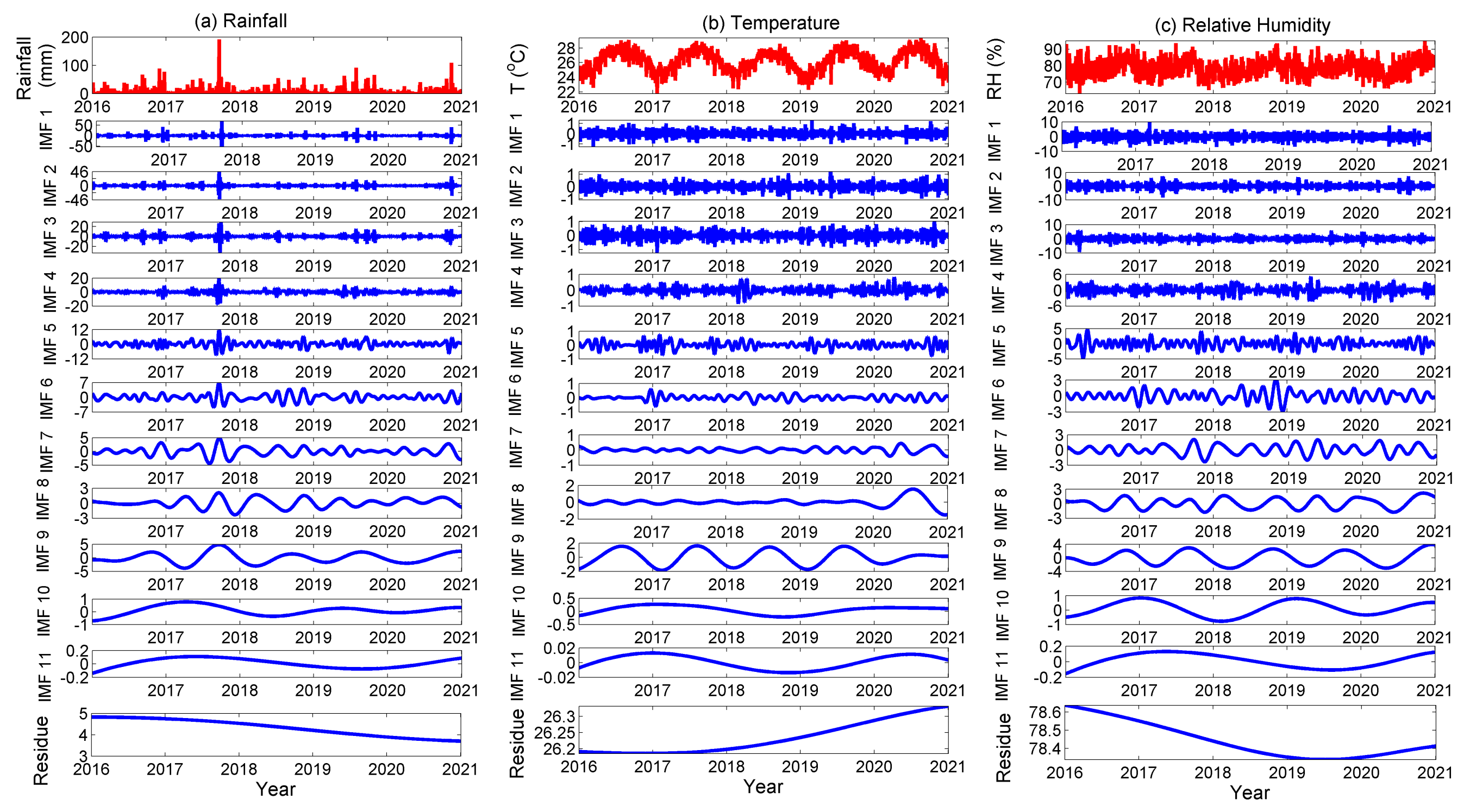
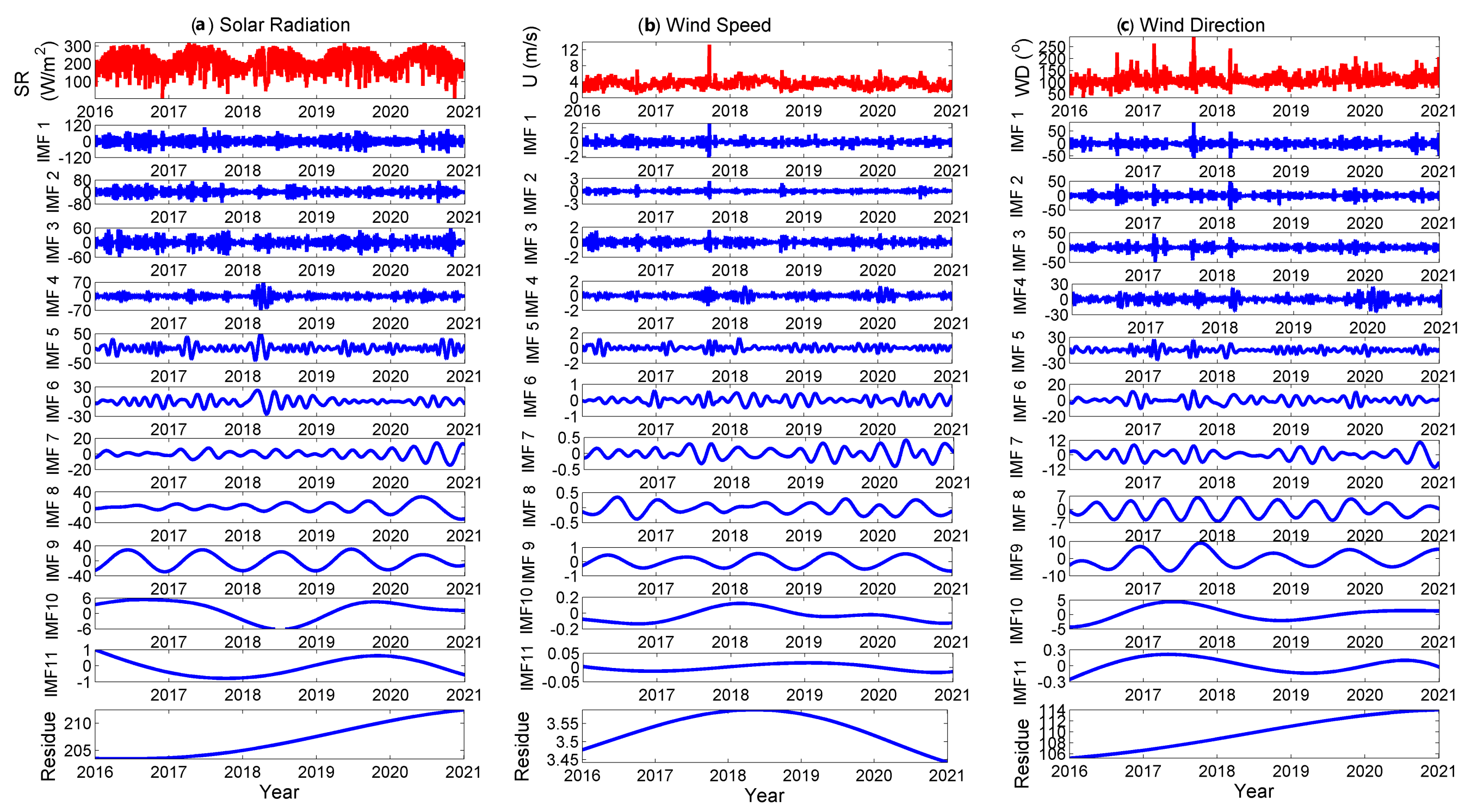
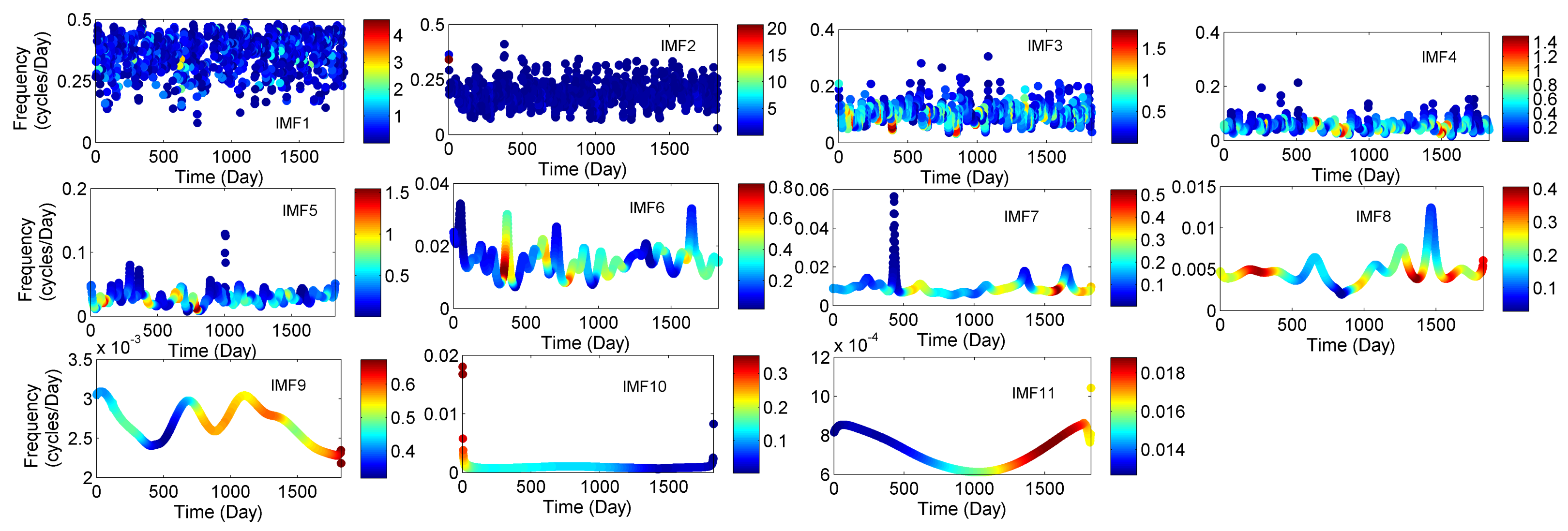
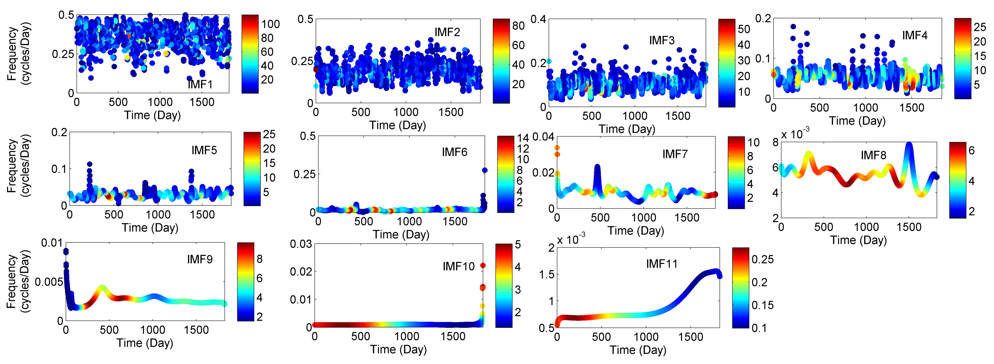
Before performing the TDIC analysis, first we applied the multi-scale decomposition using the MEMD frameworl. In Figure 3 and Figure 4, all time series data were decomposed into 11 IMFs and one residue. The first IMF mode represents the fast fluctuations, while the last mode represents the slowest fluctuations, i.e., an increase in the time scale with the mode index [50,51]. At first glance, we can notice that some residues, i.e., the overall trend of the time series, seem to exhibit the same behaviour over time: a decrease for R-, an increase for T-- and a mixture of both for U. The amplitude of these residues vary on small ranges showing that the changes in climatic regimes from one year to the next are not significant [52].
3.2. Instantaneous Frequency of Meteorological Parameters (IMFs)
To quantitatively determine the physical meaning behind the MEMD method and compare the IMFs, the mean periodicity of each IMF and their variability are presented in Table 1 for all parameters. The mean period is computed by the zero crossing method [34]. The ratio of variance of a mode (IMF or residue) to the variance of the data series (expressed in %) is computed as variability (V). Overall, the variability seems to decrease with increasing time scales. At IMF9, we notice a sudden increase in the variability. This may due to the impact of the Earth’s annual cycle [53] on different meteorological parameters.
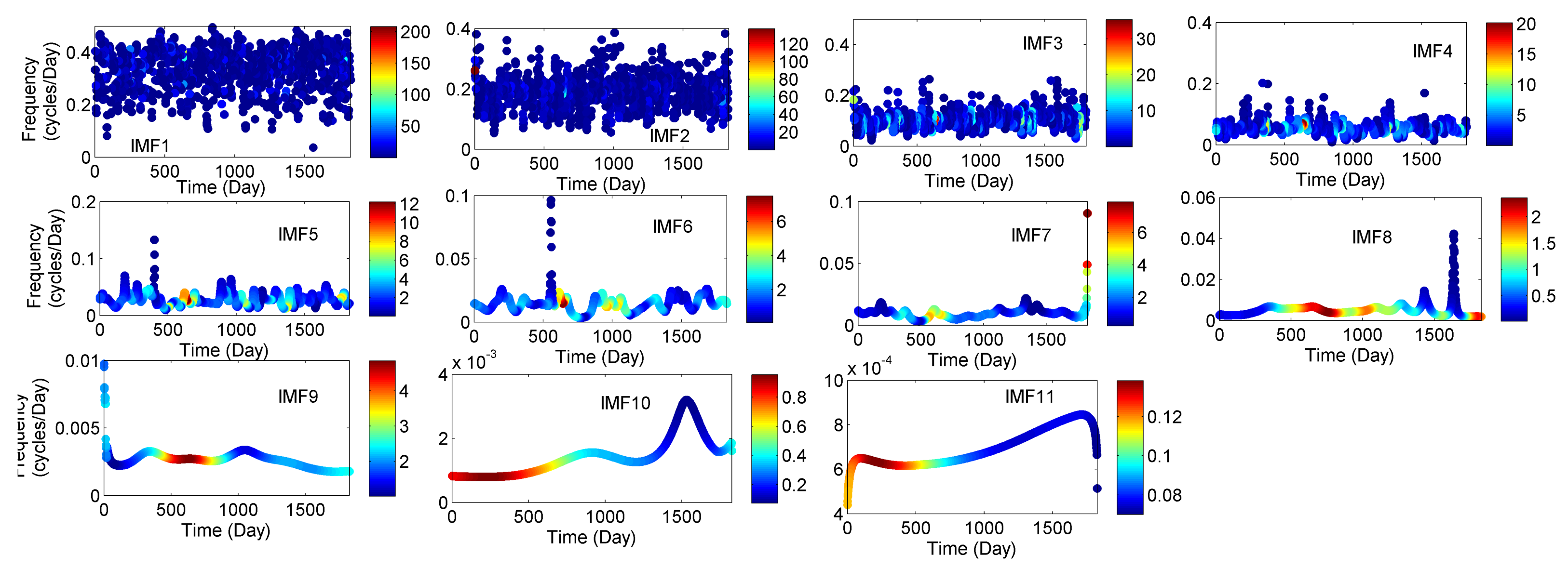
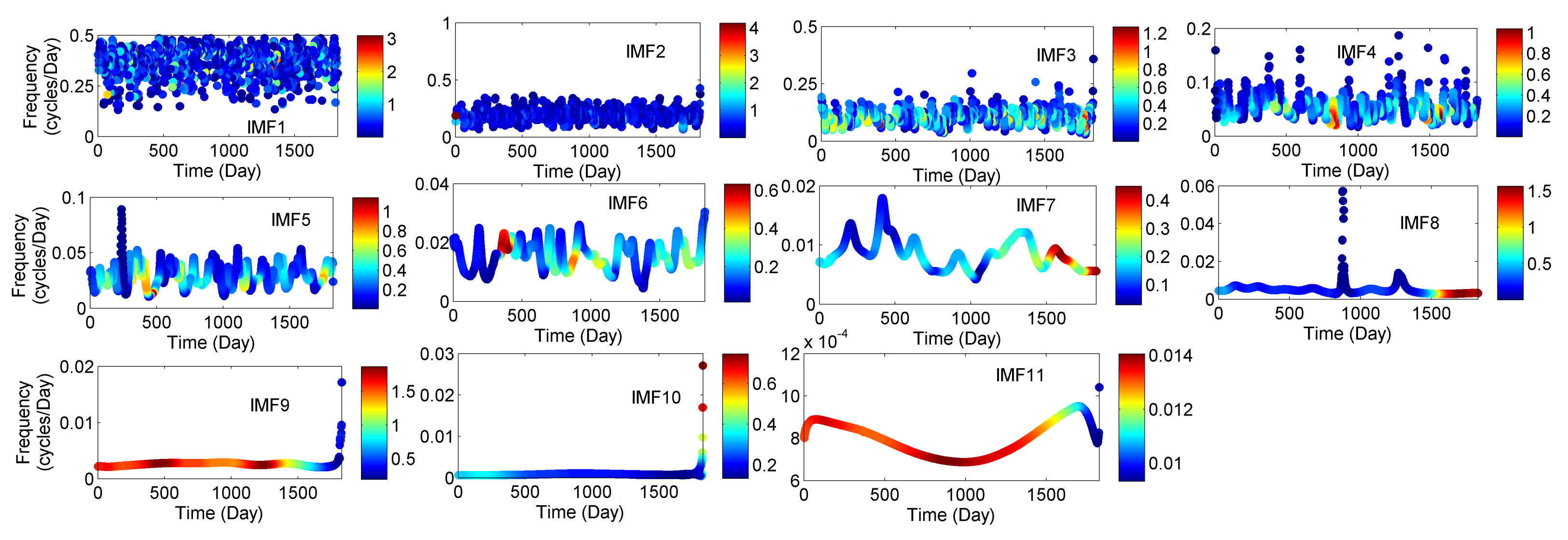
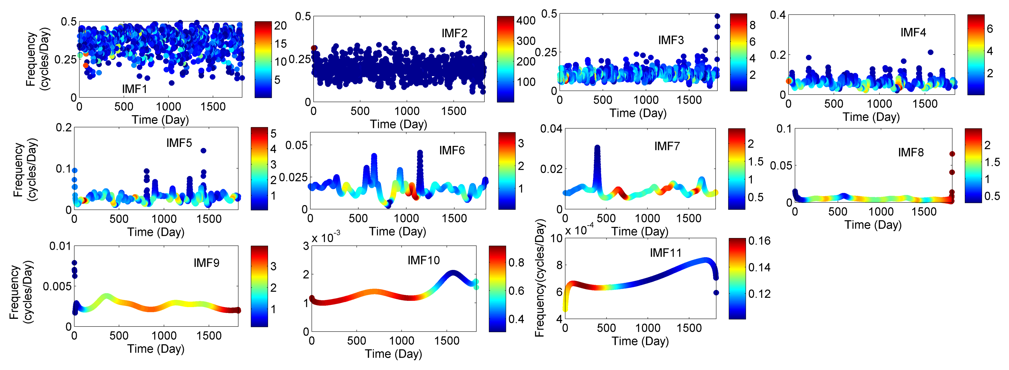
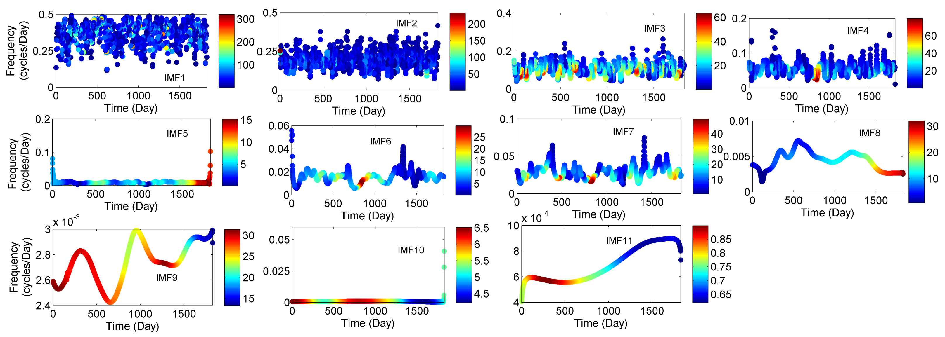
Then, HHT is applied for each IMF of all the variables and IFs and IAs are computed. The instantaneous frequency trajectories associated with the IMFs of different variables are presented in different panels of time-frequency-amplitude (TFA) spectra shown in Figure 5, Figure 6, Figure 7, Figure 8, Figure 9 and Figure 10. In the TFA spectra, the colour scale indicates the distribution of amplitude (in respective units). In general, the high amplitudes are noticed at very localized time instants in high-frequency IMFs (up to weekly scale) to seasonal time scales of ∼4 months (IMF7). The components of intra-seasonal to inter-annual periodicity are affected significantly by high amplitude. The high amplitudes are present for a longer time in the TF spectra of the IMFs of larger time scales of intra-seasonal periodicity. However, such spells pertaining to different variables do not need to be at the same time instants, indicating that the dominant contributor to the variability at different time spells may be different. Strong singularities in the form of abrupt changes in the IFs are noted in the TFA spectra of different variables in the monthly to seasonal time scales (IMF5 to IMF7). However, the period of occurrence of such abrupt shifts is also noted at different time instants, even though one of such a shift around the year of 2018 is evident, in line with the peaks in the time series of variables such as rainfall, relative humidity, wind speed and wind direction.
In the study, three types of correlation analysis were performed (i), Pearson’s correlation between the raw time series of meteorological variables with (ii), Pearson’s correlation between the modes of variables and modes of series (iii), running correlation between the modes of variables and modes of series at different scales. The overall correlation between and the parameters are presented in Table 2. One can notice that the correlations are not significant in any of the cases.
To gain better insights into the association between meteorological variables and at different time scales, Pearson’s correlations between the modes of variables and that of are computed and presented in Table 3. In Table 3, the significant correlations between and the other meteorological parameters (R-T---U) are from IMF7 to IMF11, i.e., for large time scales. Unlike the other parameters, there is no significant correlation for the residual between U and . This seems to show that is less dependent on U for the overall trend. The micro-climate of this area will therefore have a major impact on behaviour. Indeed, since the study area is in the continental island regime of the island, the trade winds speed (U) will be highly dependent on thermal convection during the day and ground cooling during the night. Consequently, behaviour will be also strongly impacted [54].
3.3. TDIC Analysis
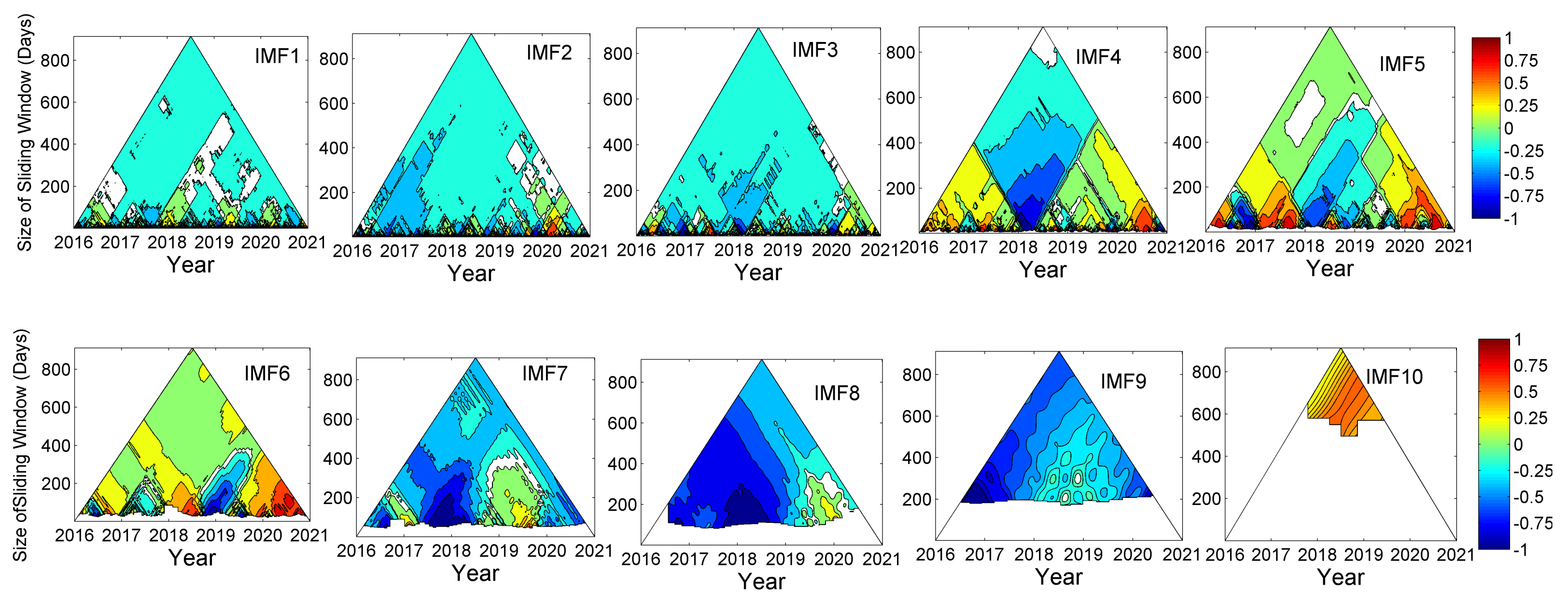
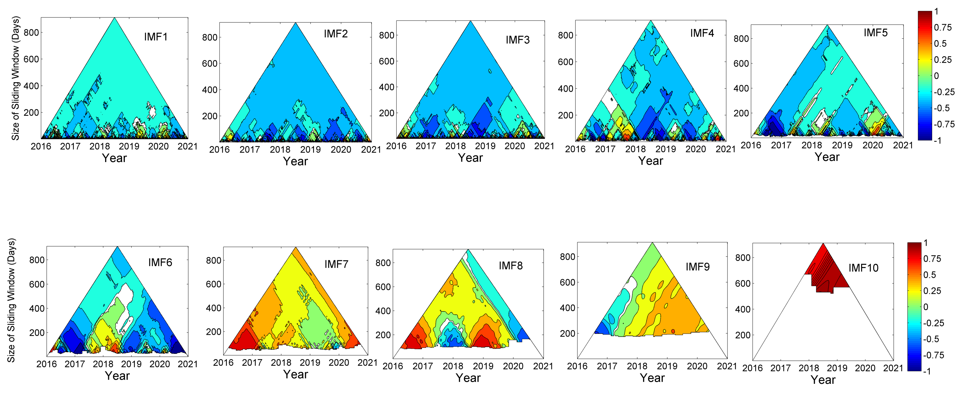
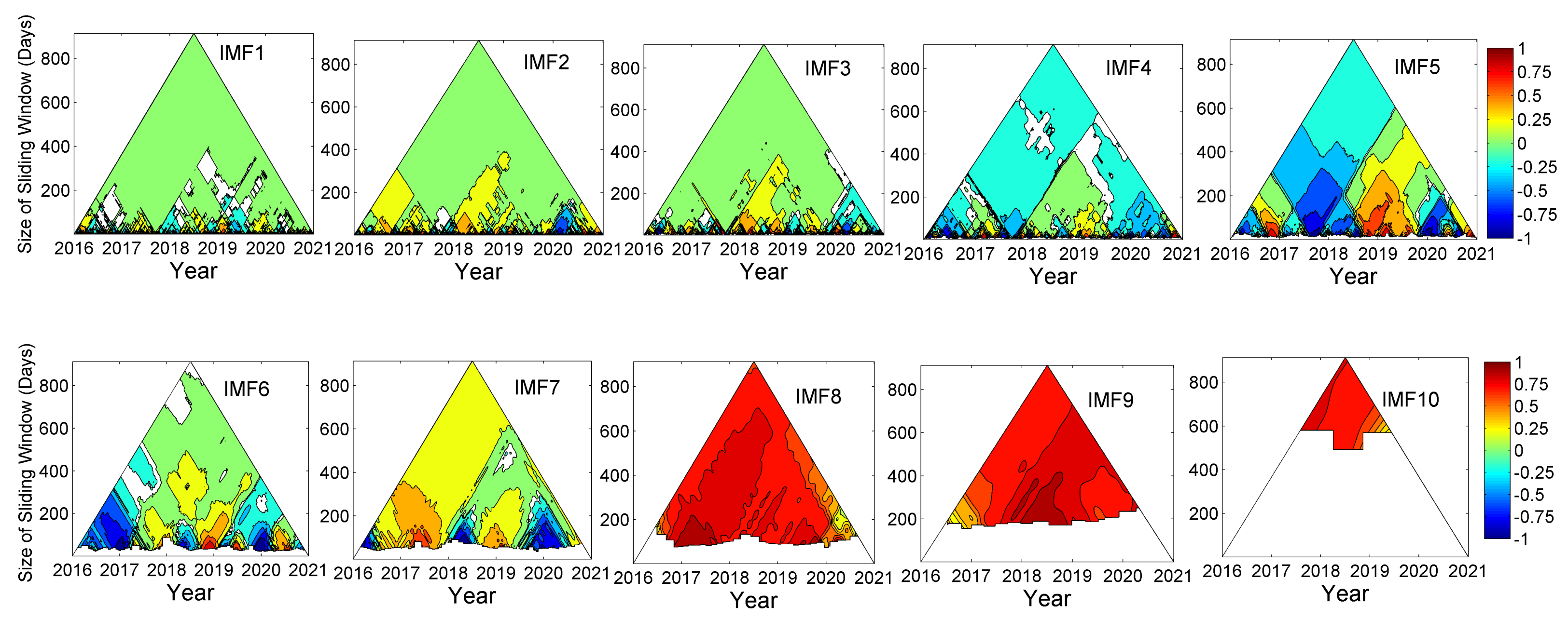
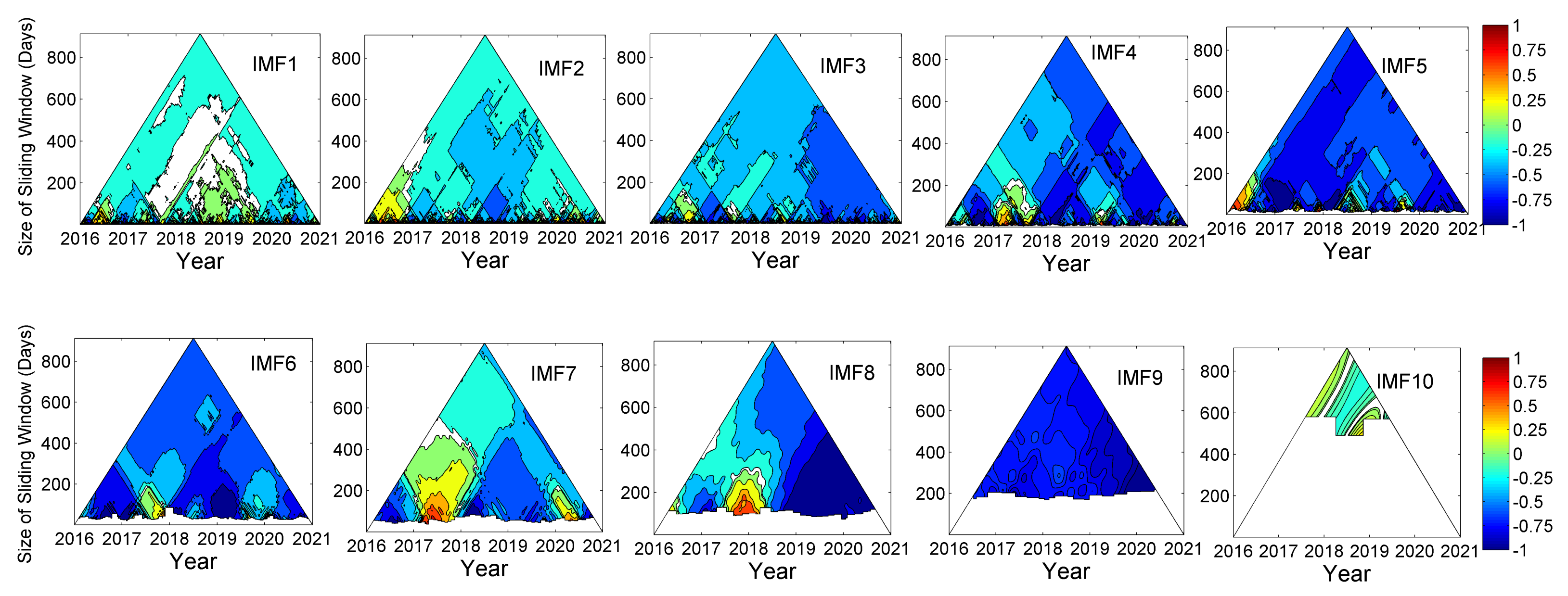
The Pearson’s correlations between the modes of meteorological variables and showed that high correlations are noted only at low-frequency modes. However, it is worth mentioning that in the computation of the overall correlation between the modes, the complete data length is considered. The reasons behind low correlation between the modes in the high-frequency scale must be investigated in detail. However, in the process of the complex behaviour of controlled by many local meteorological variables, one cannot conclude that the same low-magnitude correlation will be preserved over the complete period of observation. On the other hand, the correlation may be very strong (positive or negative) at some of the localized time spells and very weak in some other spells in some of the time scales. The effect of positive correlation in some time spells might be nullified because of the negative correlation with other spells. Moreover, it is found that the overall correlation of the different variables with is very small (Table 2). Furthermore, even if the overall correlation in some scales is strongly positive (or negative), its influence will be cancelled due to strong negative (or positive) correlations at other scales, leading to an overall low correlation between the raw time series. Therefore, it is very important to find the localized correlations, for which a running correlation method should be used. Therefore, to analyse the localized correlations between and -T--R-U over time, a TDIC analysis was performed. The TDIC analysis creates a graphic triangle, where the vertical axis is the sliding window size and the horizontal axis represents the centre position of the sliding window. The minimum size of the sliding window is the maximum instantaneous period between and the other meteorological parameters, whereas the maximum window size is the entire time range [55]. The colour bar indicates the correlation intensity between the studied variables, i.e., red and blue highlight the positive and negative correlations, respectively. White regions in the triangle indicate statistical insignificance when the correlations do not pass the Student’s t-test. Hence, the correlation is not statistically significant [28].
Overall, fom Figure 11, Figure 12, Figure 13, Figure 14 and Figure 15, one can notice there were localized positive and negative correlations between and the meteorological parameters from IMF1 (∼3 days) to IMF8 (∼7 months). The transitions in the correlation are more frequent with T and (Figure 12 and Figure 13), implying that the local meteorology may have a strong interaction with these variables to determine behaviour. This can be explained by the impact of the urban heat island (UHI) previously identified in the study area by Plocoste et al. [54] which generates an urban breeze in the evening allowing the transportation of volatile organic compounds (VOCs) emitted by LF to the urban areas opposite to the flow of the trade winds, i.e., to the west [31,54]. This urban breeze may explain the dominance of negative associations between and U in Figure 15. During this event, the UHI can reach 6 °C and generate a breeze of 1 m/s [54]. The cold and moist air coming from the mangrove will be loaded with air pollutants while passing over the LF and then cool T of the contiguous urban areas. The authors assume that this will also increase the humidity of these areas.
In Figure 11, there is also a dominance of negative correlation between and . This may be due to the impact of the diurnal cycle on the atmospheric boundary layer behaviour [56]. During the day, the mixed layer is at its maximum height, allowing the trade wind to establish itself in the study area. In the evening, the radiative cooling of the ground pushes the trade wind above the nocturnal boundary layer allowing the establishment of the urban breeze in the surface layer, thus changing behaviour.
From Figure 11, Figure 12, Figure 13, Figure 14 and Figure 15, the relationships are long range, consistent and no transition in the correlation was noticed at IMF9, i.e., annual scale. These results dynamically show the impact of the Earth’s annual cycle [53] which tends to homogenize the interactions between the meteorological parameters. IMF8 (∼7 months) to IMF10 (∼2.5 years) in Figure 14, R display a strong positive correlation with the IMFs of . R is the only variable that shows a strong positive correlation with on three consecutive time scales. As heavy rains and cyclones can cause micro-bursts that modify behaviour [57], we assume that these three large scales may correspond to periods without extreme rainy events.
The multi-scale correlation analysis can be considered as one of the potential pre-requisites for developing hybrid decomposition machine learning models for the prediction of complex time series. In such a framework, the dominant predictors in different time scales can be identified using TDIC-based multi-scale correlation analysis. Thereafter predictions can be carried out for individual scales separately and final integration will provide the prediction of wind direction. The framework is well-described and applied for the prediction of geophysical series [43,50,58]. Thus, the study has great potential for improving the predictability of wind direction, hence modelling the transportation of air pollutants.
4. Conclusions
Wind direction is a key parameter during pollutant transportation. In insular contexts, there is a wide variety of meteorological contexts due to micro-climates. For the first time in the literature, the coupled MEMD–TDIC has been used to study the dynamical relationship between wind direction () and other meteorological parameters (rainfall (R), temperature (T), relative humidity (), solar radiation () and wind speed (U)) in a multi-scale way.
Overall, localized positive and negative correlations between and the meteorological parameters were identified from ∼3 days to ∼7 months. The alternation between these correlations were more significant for T and . For and U, there is a dominance of a negative correlation with . We believe that the local micro-climate specific to the study area may explain all these behaviours. From ∼7 months to ∼2.5 years, there is a strong positive correlation between and R. We assume that these time scales correspond to a period without extreme rainy events. It is important to underline that at the annual scale, the relationships are of long range, consistent and no significant transition in correlation was found between and all the meteorological parameters. This time scale shows the influence of the Earth’s annual cycle on the behaviour of meteorological parameters.
The results obtained in this study clearly show the impact of R-T---U on over different time scales. Due to the small size of the Caribbean islands, these results are crucial because they provide information on the impact of micro-climates on behaviour. In order to develop predictive models for , the lagged influence of correlations also needs to be studied. This will be the subject of our next study using the time-dependent intrinsic cross correlation (TDICC) framework.
Author Contributions
Conceptualization, T.P. and A.S.; data curation, T.P. and A.S.; formal analysis, T.P. and A.S.; funding acquisition, T.P. and A.S.; investigation, T.P. and A.S.; methodology, T.P. and A.S.; project administration, T.P. and A.S.; resources, T.P. and A.S.; software, T.P. and A.S.; supervision, T.P. and A.S.; validation, T.P. and A.S.; visualization, T.P. and A.S.; writing—original draft, T.P. and A.S.; writing—review and editing, T.P. and A.S. All authors have read and agreed to the published version of the manuscript.
Funding
This research received no external funding.
Data Availability Statement
The data presented are available on request from the corresponding author. The data are not publicly available due to privacy or ethical reasons.
Acknowledgments
The authors thank Météo France for providing the meteorological database. Special thanks to Sylvio Laventure (geomatics specialist) for their cartographic assistance.
Conflicts of Interest
The authors declare no conflict of interest.
References
- Sharholy, M.; Ahmad, K.; Mahmood, G.; Trivedi, R. Municipal solid waste management in Indian cities—A review. Waste Manag. 2008, 28, 459–467. [Google Scholar] [CrossRef]
- Alfaia, R.G.d.S.M.; Costa, A.M.; Campos, J.C. Municipal solid waste in Brazil: A review. Waste Manag. Res. 2017, 35, 1195–1209. [Google Scholar] [CrossRef] [PubMed] [Green Version]
- Yadav, P.; Samadder, S. A global prospective of income distribution and its effect on life cycle assessment of municipal solid waste management: A review. Environ. Sci. Pollut. Res. 2017, 24, 9123–9141. [Google Scholar] [CrossRef] [Green Version]
- Nanda, S.; Berruti, F. Municipal solid waste management and landfilling technologies: A review. Environ. Chem. Lett. 2021, 19, 1433–1456. [Google Scholar] [CrossRef]
- Plocoste, T.; Jacoby-Koaly, S.; Petit, R.H.; Roussas, A. Estimation of methane emission from a waste dome in a tropical insular area. Int. J. Waste Resour. 2016, 6, 1–7. [Google Scholar] [CrossRef]
- Plocoste, T.; Jacoby-Koaly, S.; Bernard, M.; Molinié, J.; Roussas, A. Impact of a new legislation on volatile organic compounds emissions in an open landfill in tropical insular climate. Int. J. Waste Resour. 2016, 6, 2. [Google Scholar] [CrossRef]
- Abul, S. Environmental and health impact of solid waste disposal at Mangwaneni dumpsite in Manzini: Swaziland. J. Sustain. Dev. Afr. 2010, 12, 64–78. [Google Scholar]
- Sankoh, F.P.; Yan, X.; Tran, Q. Environmental and health impact of solid waste disposal in developing cities: A case study of granville brook dumpsite, Freetown, Sierra Leone. J. Environ. Prot. 2013, 2013, 665–670. [Google Scholar] [CrossRef] [Green Version]
- Yu, Y.; Yu, Z.; Sun, P.; Lin, B.; Li, L.; Wang, Z.; Ma, R.; Xiang, M.; Li, H.; Guo, S. Effects of ambient air pollution from municipal solid waste landfill on children’s non-specific immunity and respiratory health. Environ. Pollut. 2018, 236, 382–390. [Google Scholar] [CrossRef]
- Grinn-Gofroń, A.; Strzelczak, A.; Wolski, T. The relationships between air pollutants, meteorological parameters and concentration of airborne fungal spores. Environ. Pollut. 2011, 159, 602–608. [Google Scholar] [CrossRef]
- Zhang, H.; Wang, Y.; Hu, J.; Ying, Q.; Hu, X.M. Relationships between meteorological parameters and criteria air pollutants in three megacities in China. Environ. Res. 2015, 140, 242–254. [Google Scholar] [CrossRef] [PubMed]
- Ravindra, K.; Goyal, A.; Mor, S. Influence of meteorological parameters and air pollutants on the airborne pollen of city Chandigarh, India. Sci. Total Environ. 2022, 818, 151829. [Google Scholar] [CrossRef]
- Holzworth, G.C. Mixing depths, wind speeds and air pollution potential for selected locations in the United States. J. Appl. Meteorol. 1967, 6, 1039–1044. [Google Scholar] [CrossRef]
- Chan, T.L.; Dong, G.; Leung, C.W.; Cheung, C.S.; Hung, W. Validation of a two-dimensional pollutant dispersion model in an isolated street canyon. Atmos. Environ. 2002, 36, 861–872. [Google Scholar] [CrossRef]
- Plocoste, T.; Dorville, J.F.; Monjoly, S.; Jacoby-Koaly, S.; André, M. Assessment of Nitrogen Oxides and Ground-Level Ozone behavior in a dense air quality station network: Case study in the Lesser Antilles Arc. J. Air Waste Manag. Assoc. 2018, 68, 1278–1300. [Google Scholar] [CrossRef] [PubMed] [Green Version]
- Coccia, M. The effects of atmospheric stability with low wind speed and of air pollution on the accelerated transmission dynamics of COVID-19. Int. J. Environ. Stud. 2021, 78, 1–27. [Google Scholar] [CrossRef]
- Coccia, M. How do low wind speeds and high levels of air pollution support the spread of COVID-19? Atmos. Pollut. Res. 2021, 12, 437–445. [Google Scholar] [CrossRef]
- He, K.; Wang, Y.; Su, W.; Yang, H. A varying-coefficient regression approach to modeling the effects of wind speed on the dispersion of pollutants. Environ. Ecol. Stat. 2022, 29, 433–452. [Google Scholar] [CrossRef]
- Somerville, M.C.; Mukerjee, S.; Fox, D.L. Estimating the wind direction of maximum air pollutant concentration. Environmetrics 1996, 7, 231–243. [Google Scholar] [CrossRef]
- Statheropoulos, M.; Vassiliadis, N.; Pappa, A. Principal component and canonical correlation analysis for examining air pollution and meteorological data. Atmos. Environ. 1998, 32, 1087–1095. [Google Scholar] [CrossRef]
- Henry, R.C.; Chang, Y.S.; Spiegelman, C.H. Locating nearby sources of air pollution by nonparametric regression of atmospheric concentrations on wind direction. Atmos. Environ. 2002, 36, 2237–2244. [Google Scholar] [CrossRef]
- Vardoulakis, S.; Valiantis, M.; Milner, J.; ApSimon, H. Operational air pollution modelling in the UK–Street canyon applications and challenges. Atmos. Environ. 2007, 41, 4622–4637. [Google Scholar] [CrossRef]
- Wallace, J.; Corr, D.; Deluca, P.; Kanaroglou, P.; McCarry, B. Mobile monitoring of air pollution in cities: The case of Hamilton, Ontario, Canada. J. Environ. Monit. 2009, 11, 998–1003. [Google Scholar] [CrossRef] [PubMed]
- Kim, K.H.; Lee, S.B.; Woo, D.; Bae, G.N. Influence of wind direction and speed on the transport of particle-bound PAHs in a roadway environment. Atmos. Pollut. Res. 2015, 6, 1024–1034. [Google Scholar] [CrossRef]
- Zeleke, T.B.; Si, B.C. Characterizing scale-dependent spatial relationships between soil properties using multifractal techniques. Geoderma 2006, 134, 440–452. [Google Scholar] [CrossRef]
- Plocoste, T.; Euphrasie-Clotilde, L.; Calif, R.; Brute, F. Quantifying spatio-temporal dynamics of African dust detection threshold for PM10 concentrations in the Caribbean area using multiscale decomposition. Front. Environ. Sci. 2022, 10, 566. [Google Scholar] [CrossRef]
- Rehman, N.; Mandic, D.P. Multivariate empirical mode decomposition. Proc. R. Soc. Math. Phys. Eng. Sci. 2010, 466, 1291–1302. [Google Scholar] [CrossRef]
- Chen, X.; Wu, Z.; Huang, N.E. The time-dependent intrinsic correlation based on the empirical mode decomposition. Adv. Adapt. Data Anal. 2010, 2, 233–265. [Google Scholar] [CrossRef]
- Plocoste, T. Detecting the Causal Nexus between Particulate Matter (PM10) and Rainfall in the Caribbean Area. Atmosphere 2022, 13, 175. [Google Scholar] [CrossRef]
- Peel, M.C.; Finlayson, B.L.; McMahon, T.A. Updated world map of the Köppen-Geiger climate classification. Hydrol. Earth Syst. Sci. 2007, 11, 1633–1644. [Google Scholar] [CrossRef] [Green Version]
- Plocoste, T.; Jacoby-Koaly, S.; Petit, R.; Molinié, J.; Roussas, A. In situ quantification and tracking of volatile organic compounds with a portable mass spectrometer in tropical waste and urban sites. Environ. Technol. 2017, 38, 2280–2294. [Google Scholar] [CrossRef]
- Plocoste, T. Multiscale analysis of the dynamic relationship between particulate matter (PM10) and meteorological parameters using CEEMDAN: A focus on “Godzilla” African dust event. Atmos. Pollut. Res. 2022, 13, 101252. [Google Scholar] [CrossRef]
- Adarsh, S.; Reddy, M.J. Multi-Scale Spectral Analysis in Hydrology: From Theory to Practice; CRC Press: Boca Raton, FL, USA, 2021. [Google Scholar]
- Huang, N.E.; Wu, Z.; Long, S.R.; Arnold, K.C.; Chen, X.; Blank, K. On instantaneous frequency. Adv. Adapt. Data Anal. 2009, 1, 177–229. [Google Scholar] [CrossRef]
- Torres, M.E.; Colominas, M.A.; Schlotthauer, G.; Flandrin, P. A complete ensemble empirical mode decomposition with adaptive noise. In Proceedings of the 2011 IEEE International Conference on Acoustics, Speech and Signal Processing (ICASSP), Prague, Czech Republic, 22–27 May 2011; pp. 4144–4147. [Google Scholar]
- Huang, N.E.; Shen, Z.; Long, S.R.; Wu, M.C.; Shih, H.H.; Zheng, Q.; Yen, N.C.; Tung, C.C.; Liu, H.H. The empirical mode decomposition and the Hilbert spectrum for nonlinear and non-stationary time series analysis. Proc. R. Soc. Lond. Math. Phys. Eng. Sci. 1998, 454, 903–995. [Google Scholar] [CrossRef]
- Lee, T.; Ouarda, T.B. Prediction of climate nonstationary oscillation processes with empirical mode decomposition. J. Geophys. Res. Atmos. 2011, 116. [Google Scholar] [CrossRef] [Green Version]
- Iyengar, R.; Raghu Kanth, S. Intrinsic mode functions and a strategy for forecasting Indian monsoon rainfall. Meteorol. Atmos. Phys. 2005, 90, 17–36. [Google Scholar] [CrossRef] [Green Version]
- Massei, N.; Fournier, M. Assessing the expression of large-scale climatic fluctuations in the hydrological variability of daily Seine river flow (France) between 1950 and 2008 using Hilbert–Huang Transform. J. Hydrol. 2012, 448, 119–128. [Google Scholar] [CrossRef]
- Antico, A.; Schlotthauer, G.; Torres, M.E. Analysis of hydroclimatic variability and trends using a novel empirical mode decomposition: Application to the Paraná River Basin. J. Geophys. Res. Atmos. 2014, 119, 1218–1233. [Google Scholar] [CrossRef] [Green Version]
- Wu, Z.; Huang, N.E.; Long, S.R.; Peng, C.K. On the trend, detrending, and variability of nonlinear and nonstationary time series. Proc. Natl. Acad. Sci. USA 2007, 104, 14889–14894. [Google Scholar] [CrossRef] [Green Version]
- Hu, W.; Si, B.C. Soil water prediction based on its scale-specific control using multivariate empirical mode decomposition. Geoderma 2013, 193, 180–188. [Google Scholar] [CrossRef]
- Adarsh, S.; Janga Reddy, M. Evaluation of trends and predictability of short-term droughts in three meteorological subdivisions of India using multivariate EMD-based hybrid modelling. Hydrol. Process. 2019, 33, 130–143. [Google Scholar] [CrossRef] [Green Version]
- Huang, G.; Su, Y.; Kareem, A.; Liao, H. Time-frequency analysis of nonstationary process based on multivariate empirical mode decomposition. J. Eng. Mech. 2016, 142, 04015065. [Google Scholar] [CrossRef]
- Kanwal, R.P. Linear Integral Equations; Springer Science & Business Media: Berlin/Heidelberg, Germany, 2013. [Google Scholar]
- Huang, Y.; Schmitt, F.G. Time dependent intrinsic correlation analysis of temperature and dissolved oxygen time series using empirical mode decomposition. J. Mar. Syst. 2014, 130, 90–100. [Google Scholar] [CrossRef] [Green Version]
- Ismail, D.K.B.; Lazure, P.; Puillat, I. Advanced spectral analysis and cross correlation based on the empirical mode decomposition: Application to the environmental time series. IEEE Geosci. Remote Sens. Lett. 2015, 12, 1968–1972. [Google Scholar] [CrossRef] [Green Version]
- Derot, J.; Schmitt, F.G.; Gentilhomme, V.; Morin, P. Correlation between long-term marine temperature time series from the eastern and western English Channel: Scaling analysis using empirical mode decomposition. C. R. Geosci. 2016, 348, 343–349. [Google Scholar] [CrossRef]
- Plocoste, T.; Calif, R.; Jacoby-Koaly, S. Multi-scale time dependent correlation between synchronous measurements of ground-level ozone and meteorological parameters in the Caribbean Basin. Atmos. Environ. 2019, 211, 234–246. [Google Scholar] [CrossRef]
- Adarsh, S.; Reddy, M.J. Multiscale characterization and prediction of monsoon rainfall in India using Hilbert—Huang transform and time-dependent intrinsic correlation analysis. Meteorol. Atmos. Phys. 2018, 130, 667–688. [Google Scholar] [CrossRef]
- Plocoste, T.; Calif, R.; Euphrasie-Clotilde, L.; Brute, F.N. Investigation of local correlations between particulate matter (PM10) and air temperature in the Caribbean basin using Ensemble Empirical Mode Decomposition. Atmos. Pollut. Res. 2020, 11, 1692–1704. [Google Scholar] [CrossRef]
- Plocoste, T.; Pavón-Domínguez, P. Multifractal detrended cross-correlation analysis of wind speed and solar radiation. Chaos Interdiscip. J. Nonlinear Sci. 2020, 30, 113109. [Google Scholar] [CrossRef]
- Gutzwiller, M.C. Moon-Earth-Sun: The oldest three-body problem. Rev. Mod. Phys. 1998, 70, 589. [Google Scholar] [CrossRef] [Green Version]
- Plocoste, T.; Jacoby-Koaly, S.; Molinié, J.; Petit, R. Evidence of the effect of an urban heat island on air quality near a landfill. Urban Clim. 2014, 10, 745–757. [Google Scholar] [CrossRef]
- Peng, Q.; Wen, F.; Gong, X. Time-dependent intrinsic correlation analysis of crude oil and the US dollar based on CEEMDAN. Int. J. Financ. Econ. 2021, 26, 834–848. [Google Scholar] [CrossRef]
- Stull, R.B. An Introduction to Boundary Layer Meteorology; Springer Science & Business Media: Berlin/Heidelberg, Germany, 2012; Volume 13, p. 666. [Google Scholar]
- Fujita, T.T. Downbursts: Meteorological features and wind field characteristics. J. Wind. Eng. Ind. Aerodyn. 1990, 36, 75–86. [Google Scholar] [CrossRef]
- Johny, K.; Pai, M.L.; Adarsh, S. A multivariate EMD-LSTM model aided with Time Dependent Intrinsic Cross-Correlation for monthly rainfall prediction. Appl. Soft Comput. 2022, 123, 108941. [Google Scholar] [CrossRef]
Figure 1.
Map of the Guadeloupe archipelago with the locations of Météo France () indicated by a black triangle and the biggest open landfill () site indicated by a red circle. The arrows highlight the trade wind direction.
Figure 1.
Map of the Guadeloupe archipelago with the locations of Météo France () indicated by a black triangle and the biggest open landfill () site indicated by a red circle. The arrows highlight the trade wind direction.

Figure 2.
Framework of the multi-scale multidimensional correlation analysis.

Figure 3.
Results of the decomposition of different variables using the MEMD analysis for (a) rainfall (R); (b) temperature (T) and (c) relative humidity ().
Figure 3.
Results of the decomposition of different variables using the MEMD analysis for (a) rainfall (R); (b) temperature (T) and (c) relative humidity ().

Figure 4.
Results of the decomposition of different variables using the MEMD analysis for (a) solar radiation (); (b) wind speed (U) and (c) wind direction ().
Figure 4.
Results of the decomposition of different variables using the MEMD analysis for (a) solar radiation (); (b) wind speed (U) and (c) wind direction ().

Figure 5.
The time-Frequency -frequency-amplitude spectra of IMFs of rainfall.

Figure 6.
The time-frequency-amplitude spectra of the IMFs of temperature.

Figure 7.
The time-frequency-amplitude spectra of the IMFs of relative humidity.

Figure 8.
The time-frequency-amplitude spectra of the IMFs of solar radiation.

Figure 9.
The time-frequency-amplitude spectra of the IMFs of wind speed.

Figure 10.
The time-frequency-amplitude spectra of the IMFs of wind direction.

Figure 11.
TDIC plots between solar radiation () and wind direction (). The white spaces imply that correlation is not significant at the 5% level.
Figure 11.
TDIC plots between solar radiation () and wind direction (). The white spaces imply that correlation is not significant at the 5% level.

Figure 12.
TDIC plots between temperature (T) and wind direction (). The white spaces imply that correlation is not significant at the 5% level.
Figure 12.
TDIC plots between temperature (T) and wind direction (). The white spaces imply that correlation is not significant at the 5% level.

Figure 13.
TDIC plots between relative humidity () and wind direction (). The white spaces imply that correlation is not significant at the 5% level.
Figure 13.
TDIC plots between relative humidity () and wind direction (). The white spaces imply that correlation is not significant at the 5% level.

Figure 14.
TDIC plots between rainfall (R) and wind direction (). The white spaces imply that correlation is not significant at the 5% level.
Figure 14.
TDIC plots between rainfall (R) and wind direction (). The white spaces imply that correlation is not significant at the 5% level.

Figure 15.
TDIC plots between wind speed (U) and wind direction (). The white spaces imply that correlation is not significant at the 5% level.
Figure 15.
TDIC plots between wind speed (U) and wind direction (). The white spaces imply that correlation is not significant at the 5% level.


Table 1.
Periodicity () and variability (V) obtained by the MEMD analysis for all parameters. LT is for long term.
Table 1.
Periodicity () and variability (V) obtained by the MEMD analysis for all parameters. LT is for long term.
| Rainfall | Temperature | Relative Humidity | ||||
|---|---|---|---|---|---|---|
| Modes | (Days) | V (%) | (Days) | V (%) | (Days) | V (%) |
| IMF1 | 2.905 | 38.974 | 2.671 | 5.536 | 2.687 | 19.992 |
| IMF2 | 4.885 | 20.720 | 4.872 | 5.000 | 4.978 | 16.638 |
| IMF3 | 8.742 | 17.364 | 8.659 | 5.550 | 8.659 | 13.764 |
| IMF4 | 16.459 | 8.236 | 15.887 | 2.911 | 16.917 | 9.980 |
| IMF5 | 31.500 | 5.265 | 31.500 | 3.656 | 33.218 | 8.820 |
| IMF6 | 60.900 | 2.547 | 57.094 | 1.584 | 60.900 | 3.796 |
| IMF7 | 101.500 | 2.202 | 114.188 | 1.259 | 114.188 | 4.085 |
| IMF8 | 203.000 | 0.776 | 203.000 | 12.268 | 203.000 | 5.074 |
| IMF9 | 304.500 | 3.633 | 365.400 | 60.834 | 304.500 | 16.740 |
| IMF10 | 609.000 | 0.130 | 913.500 | 1.260 | 609.000 | 1.039 |
| IMF11 | 1827.000 | 0.004 | 913.500 | 0.005 | 1827.000 | 0.031 |
| Residue | LT | 0.150 | LT | 0.139 | LT | 0.041 |
| Solar radiation | Wind speed | Wind direction | ||||
| Modes | (Days) | V (%) | (Days) | V (%) | (Days) | V (%) |
| IMF1 | 2.687 | 31.998 | 2.659 | 13.060 | 2.699 | 29.116 |
| IMF2 | 4.885 | 15.998 | 4.911 | 14.761 | 4.885 | 18.601 |
| IMF3 | 8.869 | 12.871 | 8.659 | 17.381 | 8.659 | 17.494 |
| IMF4 | 17.075 | 9.077 | 16.761 | 15.065 | 16.917 | 10.567 |
| IMF5 | 34.472 | 7.192 | 32.053 | 13.015 | 32.625 | 8.337 |
| IMF6 | 60.900 | 2.249 | 63.000 | 5.008 | 60.900 | 3.432 |
| IMF7 | 107.471 | 0.941 | 107.471 | 2.962 | 101.500 | 3.068 |
| IMF8 | 228.375 | 4.901 | 203.000 | 3.214 | 182.700 | 2.666 |
| IMF9 | 365.400 | 13.829 | 365.400 | 14.635 | 365.400 | 3.752 |
| IMF10 | 913.500 | 0.547 | 913.500 | 0.685 | 913.500 | 1.121 |
| IMF11 | 1827.000 | 0.011 | 1827.000 | 0.014 | 913.500 | 0.003 |
| Residue | LT | 0.388 | 1827.000 | 0.200 | LT | 1.842 |
Table 2.
Pearson’s correlation coefficients of the raw time series between wind direction () and rainfall (R), temperature (T), relative humidity (), solar radiation () and wind speed (U).
Table 2.
Pearson’s correlation coefficients of the raw time series between wind direction () and rainfall (R), temperature (T), relative humidity (), solar radiation () and wind speed (U).
| Parameters | Pearson Correlation |
|---|---|
| vs. R | 0.11 |
| vs. T | −0.04 |
| vs. | 0.32 |
| vs. | −0.08 |
| vs. U | −0.29 |
Table 3.
Correlation between the modes of wind direction and the modes of rainfall, temperature, relative humidity, solar radiation and wind speed. Significant correlations at the 5% level are marked in bold.
Table 3.
Correlation between the modes of wind direction and the modes of rainfall, temperature, relative humidity, solar radiation and wind speed. Significant correlations at the 5% level are marked in bold.
| Rainfall | ||||||||||||
|---|---|---|---|---|---|---|---|---|---|---|---|---|
| Wind Direction | IMF1 | IMF2 | IMF3 | IMF4 | IMF5 | IMF6 | IMF7 | IMF8 | IMF9 | IMF10 | IMF11 | Residue |
| IMF1 | 0.085 | −0.003 | −0.009 | 0.003 | −0.009 | −0.008 | −0.015 | −0.003 | −0.006 | −0.005 | −0.004 | 0.006 |
| IMF2 | −0.004 | 0.166 | 0.023 | −0.004 | −0.006 | 0.006 | −0.001 | 0.011 | −0.003 | −0.003 | −0.001 | 0.002 |
| IMF3 | −0.008 | 0.004 | 0.101 | 0.021 | 0.000 | −0.015 | −0.006 | −0.001 | −0.007 | −0.004 | −0.005 | 0.010 |
| IMF4 | 0.003 | 0.000 | −0.016 | −0.050 | 0.040 | 0.003 | 0.004 | −0.003 | −0.016 | −0.017 | −0.011 | −0.019 |
| IMF5 | 0.012 | −0.015 | 0.016 | −0.007 | −0.050 | 0.047 | 0.010 | 0.022 | 0.002 | 0.017 | 0.000 | 0.006 |
| IMF6 | −0.009 | −0.020 | 0.021 | 0.015 | −0.045 | 0.023 | 0.038 | 0.045 | −0.002 | −0.020 | −0.019 | 0.007 |
| IMF7 | −0.010 | −0.007 | −0.019 | −0.008 | −0.016 | 0.009 | 0.288 | 0.054 | −0.066 | 0.031 | 0.044 | −0.008 |
| IMF8 | −0.004 | −0.006 | −0.007 | 0.007 | 0.028 | 0.056 | 0.178 | 0.690 | −0.104 | 0.036 | 0.041 | 0.144 |
| IMF9 | −0.038 | 0.004 | 0.000 | 0.009 | 0.016 | 0.031 | −0.071 | −0.006 | 0.744 | 0.115 | 0.038 | 0.056 |
| IMF10 | −0.018 | −0.002 | 0.009 | 0.003 | 0.007 | 0.026 | −0.024 | 0.014 | 0.233 | 0.816 | 0.664 | −0.014 |
| IMF11 | −0.018 | −0.001 | 0.012 | −0.002 | 0.001 | −0.002 | −0.051 | −0.004 | 0.184 | 0.765 | 0.880 | −0.318 |
| Residue | 0.004 | −0.005 | −0.015 | 0.015 | 0.007 | −0.004 | 0.048 | −0.047 | −0.097 | −0.007 | 0.228 | −0.993 |
| Wind direction | Temperature | |||||||||||
| IMF1 | −0.153 | 0.012 | 0.020 | −0.027 | 0.008 | 0.011 | 0.023 | 0.011 | −0.002 | 0.012 | 0.009 | 0.008 |
| IMF2 | 0.003 | −0.204 | −0.057 | 0.000 | 0.005 | −0.008 | 0.012 | −0.013 | 0.005 | −0.007 | −0.009 | 0.012 |
| IMF3 | 0.020 | −0.039 | −0.228 | −0.045 | −0.009 | −0.005 | 0.017 | −0.001 | −0.002 | 0.000 | −0.001 | 0.003 |
| IMF4 | 0.002 | 0.011 | −0.006 | −0.186 | −0.008 | 0.030 | 0.015 | −0.004 | −0.001 | 0.015 | 0.019 | 0.015 |
| IMF5 | 0.013 | 0.015 | −0.001 | −0.074 | −0.188 | 0.007 | 0.018 | −0.002 | 0.004 | −0.018 | −0.005 | −0.027 |
| IMF6 | 0.006 | −0.005 | 0.004 | 0.002 | 0.059 | −0.245 | −0.078 | 0.046 | −0.027 | 0.023 | 0.016 | −0.005 |
| IMF7 | 0.003 | −0.004 | 0.003 | 0.003 | 0.019 | −0.022 | 0.505 | 0.088 | 0.003 | −0.019 | −0.002 | −0.007 |
| IMF8 | 0.020 | −0.002 | 0.002 | 0.013 | 0.018 | −0.004 | 0.171 | −0.059 | −0.225 | 0.038 | 0.134 | 0.044 |
| IMF9 | −0.019 | 0.001 | 0.003 | −0.008 | 0.022 | 0.080 | −0.039 | −0.023 | 0.117 | −0.004 | 0.028 | 0.001 |
| IMF10 | −0.012 | −0.005 | −0.002 | −0.016 | 0.009 | 0.036 | −0.018 | 0.001 | 0.134 | 0.776 | 0.780 | −0.162 |
| IMF11 | −0.005 | −0.007 | −0.007 | −0.016 | 0.010 | 0.048 | −0.003 | −0.026 | 0.028 | 0.630 | 0.721 | −0.147 |
| Residue | −0.003 | 0.002 | 0.010 | −0.013 | −0.004 | 0.015 | −0.054 | 0.031 | 0.076 | 0.002 | −0.197 | 0.941 |
| Wind direction | Relative humidity | |||||||||||
| IMF1 | 0.199 | −0.004 | −0.008 | 0.014 | −0.007 | 0.005 | −0.021 | 0.004 | 0.005 | −0.012 | −0.011 | 0.002 |
| IMF2 | 0.014 | 0.386 | 0.057 | −0.004 | −0.001 | 0.002 | −0.004 | 0.012 | −0.004 | 0.002 | 0.000 | 0.003 |
| IMF3 | −0.016 | 0.041 | 0.304 | 0.063 | −0.009 | −0.004 | 0.007 | 0.018 | −0.007 | 0.002 | 0.002 | 0.012 |
| IMF4 | 0.000 | −0.006 | 0.029 | 0.345 | 0.081 | −0.007 | −0.016 | 0.014 | 0.002 | −0.021 | −0.013 | −0.029 |
| IMF5 | 0.007 | −0.013 | 0.012 | 0.045 | 0.200 | 0.088 | 0.004 | 0.016 | 0.009 | 0.017 | 0.004 | 0.019 |
| IMF6 | 0.007 | −0.004 | 0.005 | 0.009 | −0.012 | 0.151 | 0.155 | 0.017 | 0.010 | 0.017 | 0.015 | −0.003 |
| IMF7 | −0.013 | −0.004 | −0.012 | −0.008 | 0.001 | 0.011 | 0.454 | 0.084 | −0.063 | −0.001 | 0.016 | −0.017 |
| IMF8 | −0.004 | −0.003 | −0.013 | 0.007 | 0.003 | 0.007 | 0.055 | 0.398 | 0.123 | 0.003 | −0.061 | 0.119 |
| IMF9 | −0.033 | 0.001 | 0.001 | 0.011 | 0.015 | 0.039 | −0.068 | 0.030 | 0.760 | 0.111 | 0.015 | 0.093 |
| IMF10 | −0.004 | −0.010 | 0.001 | 0.017 | 0.007 | 0.075 | −0.011 | −0.014 | 0.042 | 0.107 | 0.022 | 0.010 |
| IMF11 | −0.017 | −0.003 | 0.009 | −0.002 | 0.002 | 0.003 | −0.051 | −0.016 | 0.165 | 0.753 | 0.889 | −0.309 |
| Residue | 0.003 | −0.010 | −0.025 | 0.015 | 0.012 | 0.023 | 0.020 | −0.073 | −0.119 | 0.001 | 0.271 | −0.894 |
| Wind direction | Solar radiation | |||||||||||
| IMF1 | −0.056 | −0.002 | 0.014 | −0.012 | 0.006 | 0.008 | 0.007 | 0.001 | 0.007 | 0.006 | 0.008 | −0.010 |
| IMF2 | 0.007 | −0.128 | −0.026 | 0.003 | 0.001 | −0.006 | −0.009 | −0.008 | 0.001 | −0.004 | −0.002 | −0.007 |
| IMF3 | 0.003 | −0.008 | −0.093 | 0.002 | −0.006 | 0.000 | 0.004 | −0.004 | 0.002 | 0.013 | 0.013 | −0.002 |
| IMF4 | 0.002 | 0.007 | 0.004 | −0.015 | −0.005 | 0.005 | −0.003 | −0.008 | 0.013 | 0.009 | 0.003 | 0.006 |
| IMF5 | −0.002 | −0.001 | −0.022 | 0.051 | 0.152 | 0.008 | 0.004 | 0.017 | −0.023 | −0.006 | 0.006 | −0.018 |
| IMF6 | 0.006 | 0.010 | −0.009 | −0.016 | 0.059 | 0.202 | −0.071 | 0.026 | −0.043 | −0.001 | 0.009 | 0.000 |
| IMF7 | 0.007 | −0.002 | 0.005 | 0.018 | −0.001 | −0.031 | −0.349 | −0.144 | 0.023 | −0.010 | −0.018 | 0.007 |
| IMF8 | 0.013 | 0.005 | 0.005 | −0.010 | 0.010 | −0.049 | 0.048 | −0.270 | −0.261 | 0.000 | 0.089 | −0.047 |
| IMF9 | 0.005 | −0.001 | −0.002 | −0.005 | 0.015 | 0.066 | −0.004 | −0.030 | −0.533 | −0.047 | −0.008 | −0.063 |
| IMF10 | 0.000 | −0.008 | −0.020 | −0.002 | 0.014 | 0.051 | 0.007 | −0.014 | −0.015 | 0.215 | 0.171 | −0.203 |
| IMF11 | 0.017 | −0.002 | −0.017 | −0.002 | 0.003 | 0.026 | 0.048 | −0.003 | −0.183 | −0.612 | −0.707 | 0.254 |
| Residue | −0.004 | 0.004 | 0.013 | −0.014 | −0.006 | 0.008 | −0.050 | 0.040 | 0.087 | −0.003 | −0.224 | 0.977 |
| Wind direction | Wind speed | |||||||||||
| IMF1 | −0.085 | 0.012 | 0.007 | −0.025 | 0.001 | 0.012 | 0.002 | 0.011 | −0.010 | 0.008 | 0.013 | 0.004 |
| IMF2 | 0.000 | −0.096 | −0.066 | −0.002 | 0.002 | −0.009 | 0.000 | −0.006 | 0.005 | 0.009 | 0.010 | −0.006 |
| IMF3 | 0.021 | −0.035 | −0.294 | −0.058 | −0.030 | −0.014 | 0.000 | −0.014 | −0.010 | −0.015 | −0.014 | −0.004 |
| IMF4 | −0.006 | 0.011 | −0.012 | −0.465 | −0.014 | 0.039 | 0.024 | −0.009 | −0.018 | 0.013 | 0.011 | 0.011 |
| IMF5 | 0.005 | 0.000 | 0.010 | −0.098 | −0.489 | −0.065 | −0.002 | 0.002 | 0.009 | −0.018 | −0.018 | −0.019 |
| IMF6 | −0.003 | −0.009 | 0.016 | 0.019 | −0.061 | −0.480 | −0.093 | −0.066 | −0.011 | −0.001 | −0.009 | 0.002 |
| IMF7 | 0.003 | 0.001 | −0.006 | 0.018 | −0.026 | −0.097 | −0.265 | −0.076 | −0.022 | 0.031 | 0.015 | 0.020 |
| IMF8 | 0.001 | −0.002 | 0.001 | −0.008 | −0.035 | −0.006 | −0.039 | −0.383 | −0.111 | 0.026 | 0.084 | −0.080 |
| IMF9 | 0.022 | 0.000 | −0.006 | −0.011 | −0.004 | 0.042 | 0.041 | −0.003 | −0.749 | −0.104 | −0.029 | −0.060 |
| IMF10 | −0.003 | 0.014 | 0.018 | −0.008 | −0.013 | −0.086 | 0.012 | 0.049 | 0.083 | 0.065 | 0.023 | 0.059 |
| IMF11 | 0.007 | 0.009 | 0.010 | 0.008 | −0.010 | −0.044 | 0.027 | 0.048 | −0.025 | −0.532 | −0.675 | 0.157 |
| Residue | −0.001 | 0.008 | 0.018 | −0.001 | −0.009 | −0.047 | 0.046 | 0.042 | 0.055 | 0.089 | 0.056 | −0.256 |
Disclaimer/Publisher’s Note: The statements, opinions and data contained in all publications are solely those of the individual author(s) and contributor(s) and not of MDPI and/or the editor(s). MDPI and/or the editor(s) disclaim responsibility for any injury to people or property resulting from any ideas, methods, instructions or products referred to in the content. |
© 2023 by the authors. Licensee MDPI, Basel, Switzerland. This article is an open access article distributed under the terms and conditions of the Creative Commons Attribution (CC BY) license (https://creativecommons.org/licenses/by/4.0/).
Share and Cite
MDPI and ACS Style
Plocoste, T.; Sankaran, A. Multiscale Correlation Analysis between Wind Direction and Meteorological Parameters in Guadeloupe Archipelago. Earth 2023, 4, 151-167. https://doi.org/10.3390/earth4010008
AMA Style
Plocoste T, Sankaran A. Multiscale Correlation Analysis between Wind Direction and Meteorological Parameters in Guadeloupe Archipelago. Earth. 2023; 4(1):151-167. https://doi.org/10.3390/earth4010008
Chicago/Turabian StylePlocoste, Thomas, and Adarsh Sankaran. 2023. "Multiscale Correlation Analysis between Wind Direction and Meteorological Parameters in Guadeloupe Archipelago" Earth 4, no. 1: 151-167. https://doi.org/10.3390/earth4010008