Surface Urban Heat Island and Thermal Profiles Using Digital Image Analysis of Cities in the El Bajío Industrial Corridor, Mexico, in 2020

Abstract

The Surface Urban Heat Island (SUHI) effect refers to the difference in Land Surface Temperature (LST) between an urban area and its surrounding non-urban area. LST can provide detailed information on the variations in different types of land cover. This study, therefore, analyzes the behavior of LST and SUHIs in fourteen cities in the El Bajío Industrial Corridor, Mexico, using Landsat satellite images from 2020, with QGIS software. It utilizes thermal profiles to identify the land uses that intensify LST, which are essentially those that are anthropologically altered. The results show that the increases in LST and SUHI are more pronounced in cities with greater urban conglomeration, as well as those where there are few green areas and a sizeable industrial or mixed area, with few or no bodies of water. In addition, the increase in temperature in the SUHI is due to certain crops such as vegetables, red fruits, and basic grains such as corn, wheat, and sorghum that use fallow as part of agricultural practices, located around urban areas, which minimizes natural areas with arboreal vegetation.

1. Introduction

The transformation of natural space through urbanization, which includes residential, commercial, and industrial developments, is largely responsible for its environmental conditions, including urban climatology. Urbanization processes replace land and natural areas with built surfaces, whose materials (such as concrete, asphalt, and tiles) are largely characterized by being almost impermeable. They are composed of rigid, rough elements with sharp edges, low reflectivity, and high albedo, with decreased water absorption capacity and thermal behavior conducive to heat storage and emissions [1,2,3]. These elements, together with humidity and pollutants, contribute to increasing the air temperature of cities in relation to their less urbanized environment, such as the surrounding suburban and rural areas, through a phenomenon known as the Urban Heat Island effect [3,4,5,6,7,8,9,10,11,12,13,14].

The urban heat phenomenon can also be characterized by surface temperatures. While surface temperatures can be higher and more variable than concurrent air temperatures due to the complexity of surface types in urban settings and variations in urban topography [15,16], they tend to be associated more with surface conditions, as described by [17]. The morphology and intensity of heat islands are conditioned, among other factors, by the distribution and composition of large green areas or water mirrors, which appear as relatively low-temperature areas, in comparison with the built-up surfaces of their surroundings [18,19,20]. Since surfaces heat and cool faster than air, the highest surface temperatures are observed at midday [21,22].

Urban Heat Islands (UHIs) have rarely been studied in Mexico using satellite images of various cities. Most have been explored by collecting meteorological information data in the field, especially on the ambient temperature [3,23,24,25]. However, satellite images make it possible to identify Urban Heat Islands in a more versatile way, in addition to providing more spatial and temporal information at different coverage scales, such as the local and regional, enabling one to compare the effect of each study point in a more general way. In addition, the data obtained in these images can be complemented with information such as the topography of the land and its geographical characteristics to enhance the analysis [26].

This study, therefore, focuses on studying cities within the El Bajío Industrial Corridor comprising ten metropolitan areas: Aguascalientes, Celaya, Guanajuato, La Piedad-Pénjamo, León, Moroleón-Uriangato, Querétaro, Rioverde, San Francisco del Rincón, and San Luis Potosí and the four conurbations in the municipalities of Salamanca, Irapuato, San Juan del Río, and San Miguel de Allende, delimited according to the National Urban System (Sistema Urbano Nacional, Spanish acronym SUN) 2018, Figure 1. Due to their concentration of manufacturing companies and industries, these areas have driven migration from the countryside to the city. Industrial concentration and growth have led to the development of other sectors for the benefit of workers and their families, enabling the creation of new housing developments, hospitals, schools, community centers, and department stores that improve the quality of life of local inhabitants. However, the disproportionate growth of the population, and therefore urban areas, coupled with the lack of planning in the development of sustainable localities that would reduce the negative effects on human settlements, has produced abrupt temperature changes due to greenhouse gas emissions, biodiversity loss, and deforestation and/or desertification, leading to an increase in UHIs. The general objective of this study is therefore to analyze the Surface Urban Heat Island (SUHI) in 2020 in the metropolitan cities and conurbations of the El Bajío Industrial Corridor, Mexico, and its surrounding non-urban area, and to analyze the land covers and current land uses that have triggered the increase in Land Surface Temperature. It is hypothesized that the covers that have most increased the LST and SUHI are those with the greatest anthropological intervention. To this end, remote sensing methodologies will be applied to satellite images to obtain regional knowledge of SUHI behavior in the El Bajío Industrial Corridor, Mexico, and to identify the areas in each of the study cities most vulnerable to SUHIs.

2. Materials and Methods

2.1. Materials

The limit of the cities in the study area was defined by the National Urban System (NUS) version 2018 [27], which identified the municipalities comprising the ten Metropolitan Areas: Aguascalientes, Celaya, Guanajuato, La Piedad-Pénjamo, León, Moroleón-Uriangato, Querétaro, Rioverde, San Francisco del Rincón, and San Luis Potosí, and the four conurbations: Salamanca, Irapuato, San Juan del Río, and San Miguel de Allende, all of which are located in El Bajío, Mexico, and subsequently delimited the urban areas through the Geostatistical Framework [28]. (The Geostatistical Framework is a unique and national system designed by the INEGI, which presents the division of the national territory into different levels of disaggregation to refer geographically to the statistical information of the institutional censuses and surveys and of the state units, each element of these layers has attributes of name and geostatistical key [28]).

Images from the Operational Land Imager (OLI) and Thermal Infrared Sensor (TIRS) aboard the Landsat 8 were selected for this study since, according to [29], nearly 53% of researchers have used one or more Landsat images in their SUHI studies, which underlines the importance of the Landsat constellation for SUHI research. The main advantages of using Landsat images for conducting studies related to obtaining LST and SUHIs, as noted by [29], are that they make it possible to achieve consistent, reliable, voluminous, and freely downloadable data files, in addition to the fact that they have a comparatively high resolution of 60–120 m.

Since the swath coverage of the images is 185 km x 185 km, five images were downloaded to cover the entire area of El Bajío, Mexico. Although the repeated cycle of these images is sixteen days, just one cutoff point was used for 2020. To select the download dates, the study considered the average Maximum Temperatures by State and Nationwide (2020), obtained from the National Water Commission (Comisión Nacional del Agua, Spanish acronym CONAGUA) platform, which shows that the months with Maximum Temperature for cities in El Bajío are April and May. This made it possible to visualize the images of both months and those with the lowest percentage of cloudiness were selected.

The Landsat images were downloaded from the EarthExplorer platform of the United States Geological Survey (USGS) (EarthExplorer data are free and in the public domain; data available from U.S. Geological Survey, National Geospatial Program), while the methodology for obtaining the LST and SUHIs of the Landsat images was developed using QGIS 3.18.3 a free and open-source software.

To visualize the changes in LST and SUHI by type of cover and current land use, the GlobeLand30 Earth land-cover map (the GlobeLand30 2020 is an open access product available at http://www.globallandcover.com/ (accessed on 28 December 2022)) was used as an input, making use of its most recent version created in 2020 in tiles N13_20 and N14_20. This consists mainly of multispectral 30 m images, including TM5, ETM+, and OLI multispectral images from Landsat (USA), as well as China’s Environment and Disaster Reduction Satellite HJ-1 imagery and GF-1 16-m resolution multispectral imagery [30], and it is classified into ten land cover classes: crops, trees and forests, grasslands, bushes/shrubs, wetlands/accumulated vegetation, water bodies, tundra, built-up areas, bare soil, and permanent snow and ice. Additionally, the coverage of built-up areas of GlobeLand 30 was recategorized to integrate more categories within the cities, complementing it with current land uses.

Information was extracted on the limits of the blocks comprising each of the cities in the study area from the shapefiles of the massive download page of the National Housing Inventory (Inventario Nacional de Vivienda, Spanish acronym INV, 2010) and the National Statistical Directory of Economic Units (Directorio Estadístico Nacional de Unidades Económicas, Spanish acronym DENUE). The files were extracted on September 2016, from the website https://www.inegi.org.mx/app/descarga/?ti=13ag=01 (accessed on 28 December 2022), where the locations of economic activities were considered according to the INEGI Classification of Activities, based on the North American Industrial Classification, SCIAN 2007, and the list of blocks with residential housing.

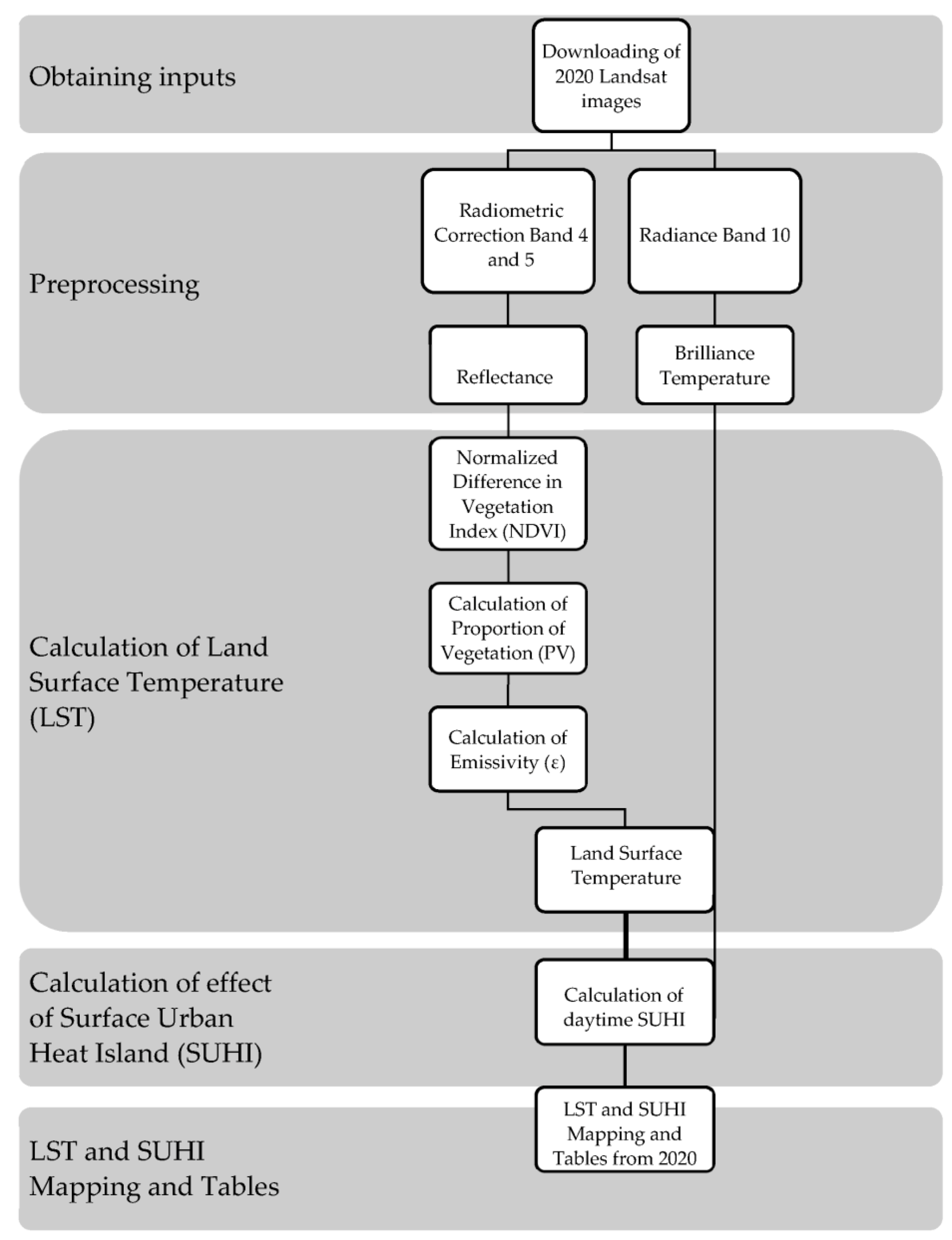
2.2. Methodology for Obtaining Land Surface Temperature and Surface Urban Heat Islands from Landsat Images

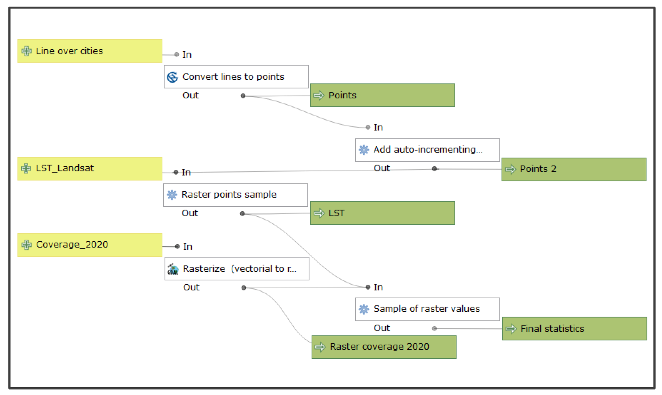
Figure 2 shows the methodology for obtaining Land Surface Temperature and Surface Urban Heat Islands from Landsat images. The steps consist of downloading the images and atmospheric and radiometric corrections in the corresponding bands, calculating the Normalized Difference Vegetation Index (NDVI) and LST, obtaining the SUHIs, and mapping and obtaining the statistics.

Obtaining inputs: As depicted in

Table 1. Characteristics of Landsat Data Corresponding to the El Bajío Region, May 2020.

Route	Row	ID	Date Obtained	Cloud Cover
029	045	LC08_L1TP_029045_20200512_20200820_02_T1	05/12/2020	0.03
028	045	LC08_L1TP_028045_20200521_20200820_02_T1	05/21/2020	0.21
027	046	LC08_L1TP_027046_20200514_20200820_02_T1	05/14/2020	1.24
028	046	LC08_L1TP_028046_20200521_20200820_02_T1	05/21/2020	0.03
027	045	LC08_L1TP_027045_20200514_20200820_02_T1	05/14/2020	3.04

, the Landsat products were downloaded from the EarthExplorer platform. The search criteria used to download the dataset for this study correspond to the weather information provided by the Comisión Nacional del Agua (Comisión Nacional del Agua, Spanish acronym, CONAGUA, 2020) database [31]. Where it is observed that the hottest months corresponding to the Bajío area are April and May, thus selecting the images closest in time and best visualized, i.e., with little or no cloud cover. The acquired data belong to level 1, which are orthorectified products. They consist of quantified data and scaled, calibrated Digital Numbers (DN) representing multispectral image data obtained through both the Operational Land Imager (OLI) and the Thermal Infrared Sensor (TIRS). The products are presented in a 16-bit positive integer format (scaled to 55,000 gray levels) and can be rescaled to Top of Atmosphere (TOA) reflectance and/or radiance using radiometric change of scale coefficients provided in the product metadata file (MTL file). The MTL file also contains the thermal constants required to convert thermal infrared sensor (TIRS) data to the brightness temperature in the satellite [32].

Spectral Radiance in OLI and TIRS Sensor: Images are processed in absolute radiance units using 32-bit floating-point calculations. These values are converted to 16-bit integer values in the finished Level 1 product. They can then be converted to spectral radiance using the reflectance scale factors provided in the metadata file [33]:

$$L_{\lambda }=M_L{Q}_{cal }+A_L$$

(1)

where

$L_{\lambda }$ = The spectral radiance value of (TOA) measured in values of (Watts/(${\mathrm{m}}^2$* srad * $\mathsf{\mu }\mathrm{m}$)).

$M_L$ = The specific multiplicative scaling factor (RADIANCE_MULT_BAND_x, where x is the number of the band).

$A_L$= The specific additive scaling factor obtained from the metadatum (RADIANCE_ADD_BAND_x, where x is the number of the band).

$Q_{cal }$ = Standard product quantified and calibrated by pixel values (DN). This value refers to each of the bands in the image.

Top of Atmosphere Reflectance (TOA) in OLI sensor: The entire 16-bit values in the Level 1 product can also be transformed into TOA reflectance. The following equation is used to turn Level 1 DN values into reflectance [33]:

$$\rho \lambda \prime =M_{\rho } * Q_{cal }+A_{\rho }$$

(2)

where

$\rho \lambda \prime$= TOA planetary reflectance, without correcting for the solar angle.

$M_{\rho }$ = Multiplicative scaling factor for metadata scaling (REFLECTANCE_MULT_BAND_x, where x is the band number).

$A_{\rho }$= Additive scaling factor based on metadata (REFLECTANCE_ADD_BAND_x, where x is the band number).

$Q_{cal }$ = Quantified and calibrated product pixel values (DN).

One should consider that $\rho \lambda \prime$ does not have a correction for the solar angle. Therefore, to obtain TOA reflectance in the sun angle, the following conversion should be used:

$$\rho \lambda =\frac{\rho \lambda \prime }{cos\left({\theta }_{SZ}\right)}=\frac{\rho \lambda \prime }{sin\left({\theta }_{SE}\right)}$$

(3)

where

$\rho \lambda$ = Planetary TOA reflectance.

${\theta }_{SE}$ = Local solar elevation angle; the sun elevation angle of the center of the scene in degree is provided by the metadata as (SUN_ELEVATION).

${\theta }_{SZ}$ = Local solar zenith angle; ${\theta }_{SZ}$ = 90° − ${\theta }_{SE}$.

Obtaining the Brightness Temperature: To calculate the Land Surface Temperature, it is necessary to obtain the brightness temperature of the thermal bands based on the radiance result. The brightness temperature is the effective temperature seen by the satellite under the assumption of unit emissivity [33]. The conversion equation is as follows:

$$T=\frac{k_2}{ ln(\frac{k_1}{L_{\lambda }}+1)}$$

(4)

where

$T$ = Brightness temperature of Top of Atmosphere.

$L_{\lambda }$ = TOA spectral radiance (Watts/(${\mathrm{m}}^2$ * srad * $\mathsf{\mu }\mathrm{m}$)).

$k_1$ = Specific thermal conversion content of metadata band(K1_CONSTANT_BAND_x, where x is the thermal band number).

$k_2$ = Specific thermal conversion content of metadata band (K2_CONSTANT_BAND_x, where x is the thermal band number).

Threshold Method based on NDVI to calculate Emissivity: Surface emissivity is a measure of the inherent efficiency of the surface, since it converts thermal energy into radiant energy over the surface. It depends on the composition, roughness, and moisture content of the surface and the observation conditions, in other words, the wavelength, pixel resolution, and viewing angle [34]. Thermal infrared emissivity is therefore an essential parameter for both surface characterization and atmospheric correction methods. The mapping of emissivity from satellite data is therefore a key issue to resolve. The main problem is temperature coupling and the effect of emissivity on thermal radiances [35].

To calculate emissivity, [36] found a high correlation between the emissivity measurement and the Normalized Difference Vegetation Index (NDVI) derived from reflectance in the red and near-infrared bands. This relationship is of potential use in sensors with infrared thermal bands because the NDVI can easily be derived from radiometric spectral measurements found on board many of the operational meteorological satellites. Accordingly, various approaches have been used to predict the emissivity of the Earth’s surface from NDVI values [35,36,37]. Therefore, in this study, the Normalized Difference Vegetation Index (NDVI) Threshold method used to calculate the emissivity of the Earth’s surface was chosen. It is worth recalling that NDVI is defined as equation 5 [38].

$$NDV I=\frac{{\rho }_2-{\rho }_1}{{\rho }_2+{\rho }_1}$$

(5)

where

${\rho }_2$: the reflectance measured in near-infrared, and ${\rho }_1$: the reflectance corresponding to red wave bands.

For Landsat OLI 8, it is:

$$NDV I=\frac{NIR\left(band5\right)-R\left(band4\right)}{NIR\left(band5\right)+R\left(band4\right)}$$

(6)

Once the NDVI has been obtained, the threshold method uses certain NDVI values (Thresholds) to distinguish between soil pixels (NDVI<NDVIs) and complete vegetation pixels (NDVI>NDVIv). Therefore, for pixels composed of soil and vegetation (mixed pixels, NDVIs ≤ NDVI ≤ NDVIv), the method uses the following equation [37].

$${\epsilon }_{\lambda }={\epsilon }_{\upsilon \lambda }{P}_{\upsilon }+{\epsilon }_{s\lambda }(1-P_{\upsilon }) + C_{\lambda }$$

(7)

where ${\epsilon }_{\upsilon }$ and ${\epsilon }_s$ are, respectively, soil emissions and vegetation; $P_{\upsilon }$ is the proportion of vegetation (also called fractional vegetation cover, FVC); and C is a term that considers the cavity effect due to surface roughness (C = 0 for flat surfaces). The proportion of vegetation is obtained through the equation [39]:

$$P_{\upsilon }={\left(\frac{NDVI-NDV{I}_S}{NDV{I}_V-NDV{I}_S}\right)}^2$$

(8)

where $NDV{I}_S$ = 0.2 y $NDV{I}_V$ = 0.5 for global conditions [40]. However, these values can be obtained from the NDVI histogram [41]. Using the histogram methodology designed by [41], the thresholds for each urban area were obtained in the El Bajío area, as shown in

Table 2. Thresholds from NDVI for calculating surface emissivity.

Metropolitan or Conurbated Area	NDVIs	NDVIv
* Aguascalientes	0.065086	0.565007
	0.0631847	0.537497
Guanajuato	0.112763	0.623928
Celaya	0.122759	0.696545
San Miguel de Allende	0.06	0.602271
Salamanca	0.0957022	0.695735
San Francisco del Rincón	0.12534	0.69975
León	0.0739849	0.646419
Irapuato	0.0851054	0.590401
La Piedad Pénjamo	0.125289	0.534888
Moroleón	0.08	0.502058
Querétaro	0.102353	0.622047
San Juan del Rio	0.115708	0.58884
Rioverde	0.188243	0.614252
San Luis Potosí	0.0652032	0.559044

* For the metropolitan area of Aguascalientes, two images were used, as a result of which different thresholds were used for each image.

.

Finally, using the geometric model proposed by authors [42], the cavity term ($C_{\lambda }$) for a mixed area and a close view of the nadir is given by the value:

$$C_{\lambda } =(1-{\epsilon }_{s\lambda }){\epsilon }_{\upsilon \lambda }F\prime (1-P_{\upsilon })$$

(9)

where $F$ is a geometric factor that varies between zero and one, depending on the geometric distribution of the surface. Given that $F\prime$ cannot be estimated from remote VNIR/TIR perception data, a mean value is usually chosen.

Land Surface Temperature: The Land Surface Temperature was calculated using the equation proposed by [43]:

$$T_S=\frac{BT}{1+\left[\left(\lambda BT/\rho \right) ln{\epsilon }_{\lambda }\right]}$$

(10)

where λ = 10.895 is equal to the wavelength of the radiance emitted; ${\epsilon }_{\lambda }$ is the emissivity calculated and $\rho$ = h$\frac{c}{\sigma }=1.438\times {10}^{-2} \mathrm{mk}$, whereby $\sigma$ is Boltzmann’s constant (${1.3810}^{23}$ J/K), h is Planck (${6.62610}^{34}$ Js); and $c$ is the speed of light (${2.99810}^8$ m/s) [44]. The result is obtained in Kelvin degrees, as a result of which the value of −273.15 is subtracted to convert it to Celsius degrees.

Surface Urban Heat Islands: From the LST calculated in equation [10] and converted to degrees Celsius in the Landsat Diurnal images, the SUHI was obtained using the following equation:

$$LS{T}_{}I \left(°C\right)-LS{T}_{}O \left(°C\right)=SUHI \left(°C\right)$$

(11)

$LS{T}_{}I \left(°C\right)$= Corresponds to the value obtained from the LST of each pixel within the metropolitan or conurbation area.

$LS{T}_{}O \left(°C\right)$= The average LST outside the metropolitan or conurbation area in a defined area of 10 km around each city.

The SUHIs were obtained by the difference in each pixel of the land surface temperature within the metropolitan or conurbation area minus the average LST in a 10 km zone of influence outside the urban area, obtaining a positive SUHI where the Surface Temperature has increased inside the cities. Subsequently, the results were plotted, and each city’s minimum, maximum, and average values were tabulated.

2.3. Transects

The use of transects in the various types of cover and soil is proposed since, as mentioned earlier [44], the profiles will help to explain the factors that shape the thermal landscape of the city. Figure 3 shows the steps that will be taken throughout this subsection.

2.3.1. Description of Categorization of El Bajío Cities for Transect Plotting

For the transect plotting, straight lines were drawn over each city, considering the 10 km buffer around the urban localities within the metropolitan areas and conurbations. Straight lines were drawn, attempting to go through extreme temperature points and diverse types of land cover and current land use. Distances were subsequently established by city size to place points along the lines and obtain the resulting LST and SUHI values as well as the type of cover coinciding with those points.

Cities were grouped according to the length of the lines considered for the transects and depending on the separation distance between the points placed on the straight lines, taking three groups into account: three kilometers for the metropolitan cities of Querétaro, León, Celaya, and La Piedad-Pénjamo, two kilometers for the metropolitan cities of San Luis Potosí, Aguascalientes, and Guanajuato, and one and a half kilometers for the metropolitan cities of Rioverde, Moroleón-Uriangato, San Francisco del Rincón, and the conurbated cities of San Juan del Río, Irapuato, Salamanca, and San Miguel de Allende. These distances between points were selected to obtain between 15 and 30 points per line to make the transect graphs, to ensure that there was sufficient information without saturating the graphs or hampering their interpretation.

2.3.2. Land Cover and Current Land Use

To obtain a sample of the transects, it was necessary to identify the land cover and current land use in the study area to determine the behavior of the daytime LST in Landsat in the various categories, and thereby identify how daytime LST interacts with current land cover and use in El Bajío, Mexico. To this end, each state’s official census information from the National Housing Inventory (Inventario Nacional de Viviendas, Spanish acronym INV, 2010) was extracted and used. Information on the blocks was subsequently combined with the number of dwellings, restricting it to an area containing both metropolitan and suburban and buffer areas. It was applied to regions in the El Bajío Industrial Corridor, highlighting the VIV0 column, referring to the number of houses for residential use in its respective table. A zero in the box indicates that there is no dwelling assigned as a residence. In the case of the DENUE, given that it specifically marks the location of the different lines of business, the information was subdivided by degree of sector, according to the INEGI Classification of Activities, based on the North American Industrial Classification, SCIAN 2007, where attributes were selected for each case:

• 11. PRIMARY ACTIVITIES. Natural resource exploitation.
• 21–23. SECONDARY ACTIVITIES. Transformation of goods such as mining, electricity, water, gas, and construction.
• 31–33. SECONDARY ACTIVITIES. Transformation of goods in manufacturing industries.
• 43–49. TERTIARY ACTIVITIES. Distribution of goods such as trade and transportation.
• 51–81. TERTIARY ACTIVITIES. These include services and information management.
• 93.TERTIARY ACTIVITIES. Government.

GlobeLand30 types of land cover were combined with the current land uses to identify each of the changes in LST of the landscapes present inside and outside the metropolitan and suburban areas. The following steps were taken to incorporate the inputs:

• The DENUE points were incorporated by an analysis of proximity to the blocks. They were therefore converted from points to polygons to identify the blocks in which economic activities were located.
• The blocks were subsequently classified according to the number of residential dwellings as well as the economic activity or activities that take place within them,

  Table 3. Classification of Current Land Use according to INEGI Data.

  Code	Current Type of Land Use	Contents
  1	Housing	Blocks with housing for purely residential use
  2	Other uses	Blocks without housing containing secondary activities such as the transformation of goods such as mining, electricity, water, gas, and construction or tertiary government activities
  3	Industry	Blocks without housing that contain secondary goods transformation activities in manufacturing industries
  4	Mixed	Blocks with housing and secondary activities involving the transformation of goods in manufacturing industries
  5	Mixed specialized	The specialized mixed category includes secondary activities involving the transformation of goods in manufacturing industries, as well as tertiary activities that include services and information management
  6	Trade and services	This category includes tertiary activities involving the distribution of goods such as trade, transportation, services, and information management

  .

A category of roads was also constructed by adapting the GlobeLand30 land cover to the size of urban locations, and block areas were subtracted to obtain the roads in polygons. In addition, green areas available in the 2017 Geostatistical Framework were included, comprising objects such as airstrips and medians. Finally, the GlobeLand30 types of cover were integrated with current land use classes and road and green area categories. Once the data had been incorporated, the resulting layer was rasterized.

2.3.3. Transect Design

Once the data resulting from the Landsat LST had been obtained, as well as the layer resulting from the integration of land cover and current land uses, the layers were superimposed over the study area, including the buffer area, and four transects were drawn per city. Every attempt was made to go through the diverse types of cover and certain points of interest within each urban area, such as airports, heat-insulating roofs, bodies of water, and green areas.

Subsequently, obtaining points on the transects separated by the estimated distance of 3, 2, and 1.5 km depending on the city was automated within the processing of the QGIS tool modeler to achieve the sample of raster values of LST, types of cover, and current land use. Figure 4 shows a diagram with the procedure and the tools used for generating points in the transects and extracting values from the rasters.

Once the tools had been automated, this made it possible to process the cities to which the same distances were going to be applied and reduce processing times. Finally, the samples of values were exported in tables to graph the results of the data obtained.

3. Results

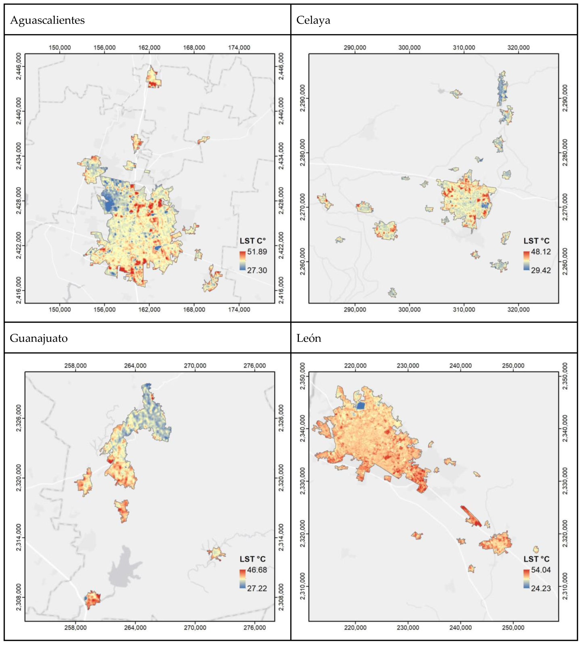
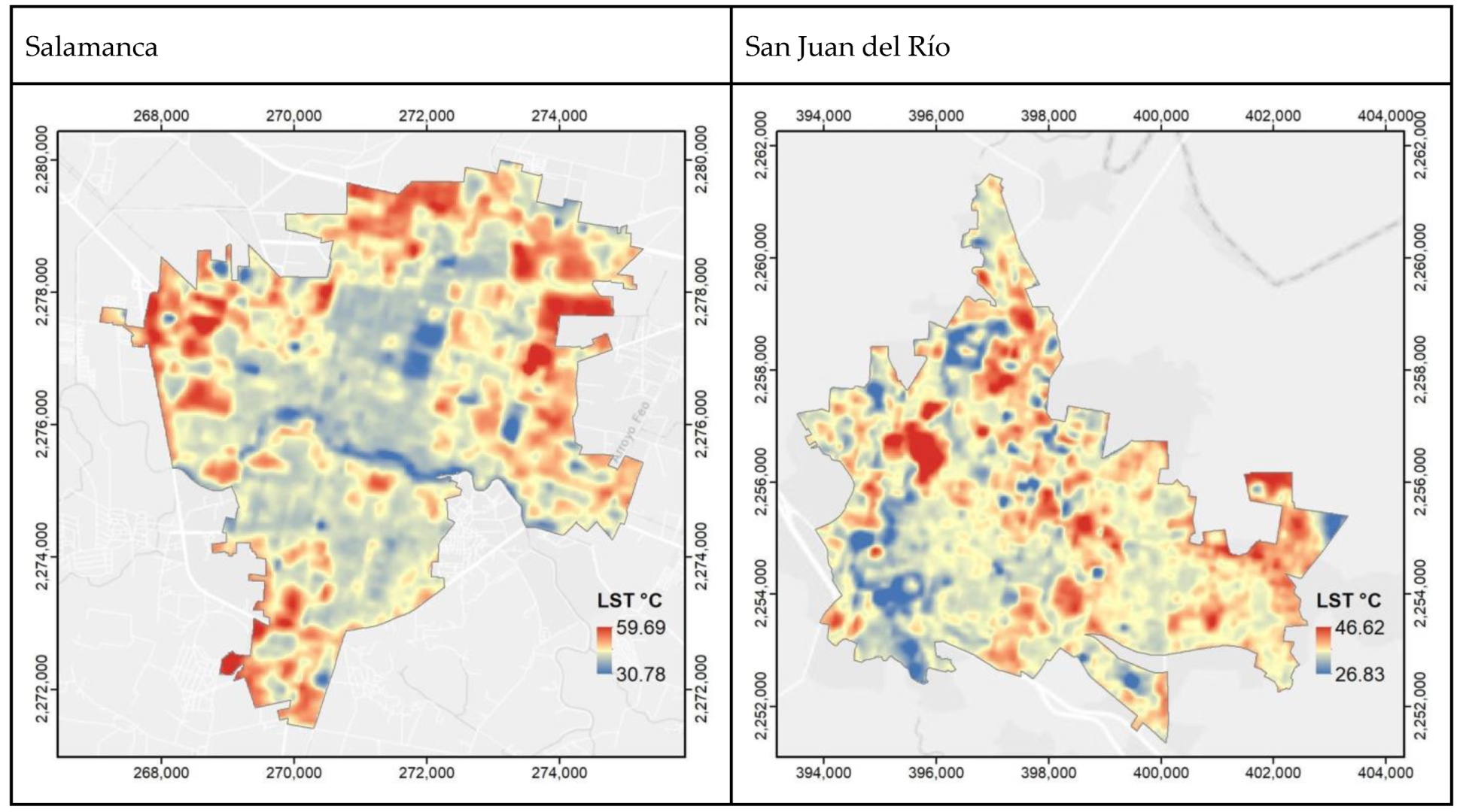
3.1. Landsat Daytime Land Surface Temperature 2020

Land Surface Temperatures obtained with Landsat images for each metropolitan area and conurbation are detailed in Appendix A.1; this shows the behavior of the daytime LST obtained from the Landsat images of the metropolitan cities and conurbations of El Bajío, Mexico. The Landsat images have higher resolution and show the areas with high or low LST in greater detail. Within the urban area of the cities, those with the maximum temperatures are the conurbation of Salamanca (59.7 °C) and the conurbations of León (53.1 °C) and Irapuato (52.7 °C), while Querétaro (21.6 °C) and León (24.3 °C) are the cities with the minimum LST. It is worth noting that, although the metropolitan area of Querétaro is one of the largest, most industrial cities in El Bajío, it has the lowest temperatures, due to the bodies of water inside the city. The opposite is true of the conurbation of Salamanca which, although the Lerma River runs through it, has a high LST identified in crop areas. In regard to the outside of the urban area of each city, the LST was obtained within a 10 km buffer.

The exterior of the urban area records lower daytime LST in all cities, since, it does not exceed the minimum LST of 30 °C, unlike the interior. It also has lower maximum LSTs than the interior area. As one would expect, areas close to bodies of water have minimum temperatures, as in the city of Querétaro, both inside and outside the urban area; although, the presence of thermal construction materials or specific buildings also causes minimum LSTs as in the metropolitan area of Aguascalientes, both inside and outside the urban area.

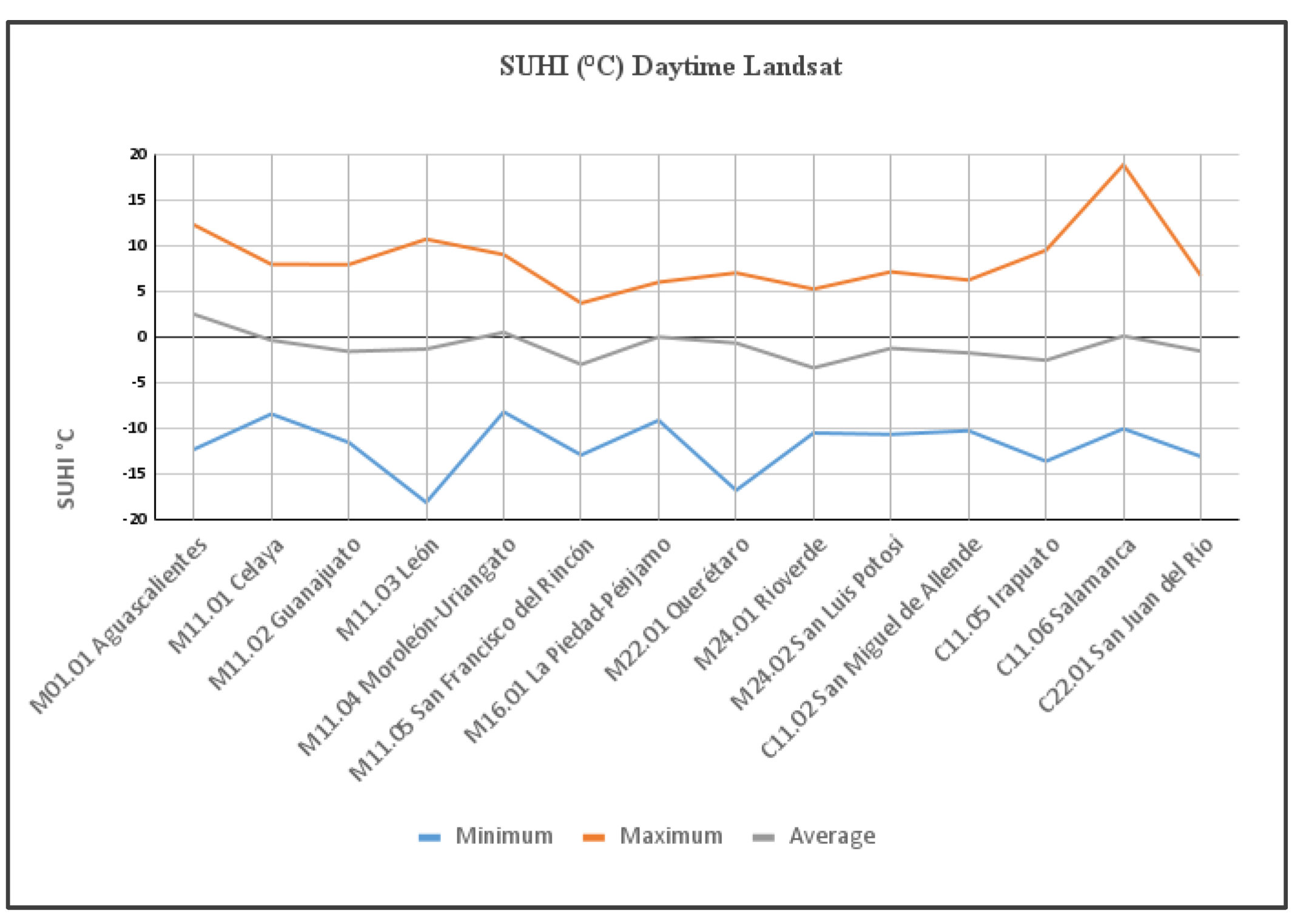
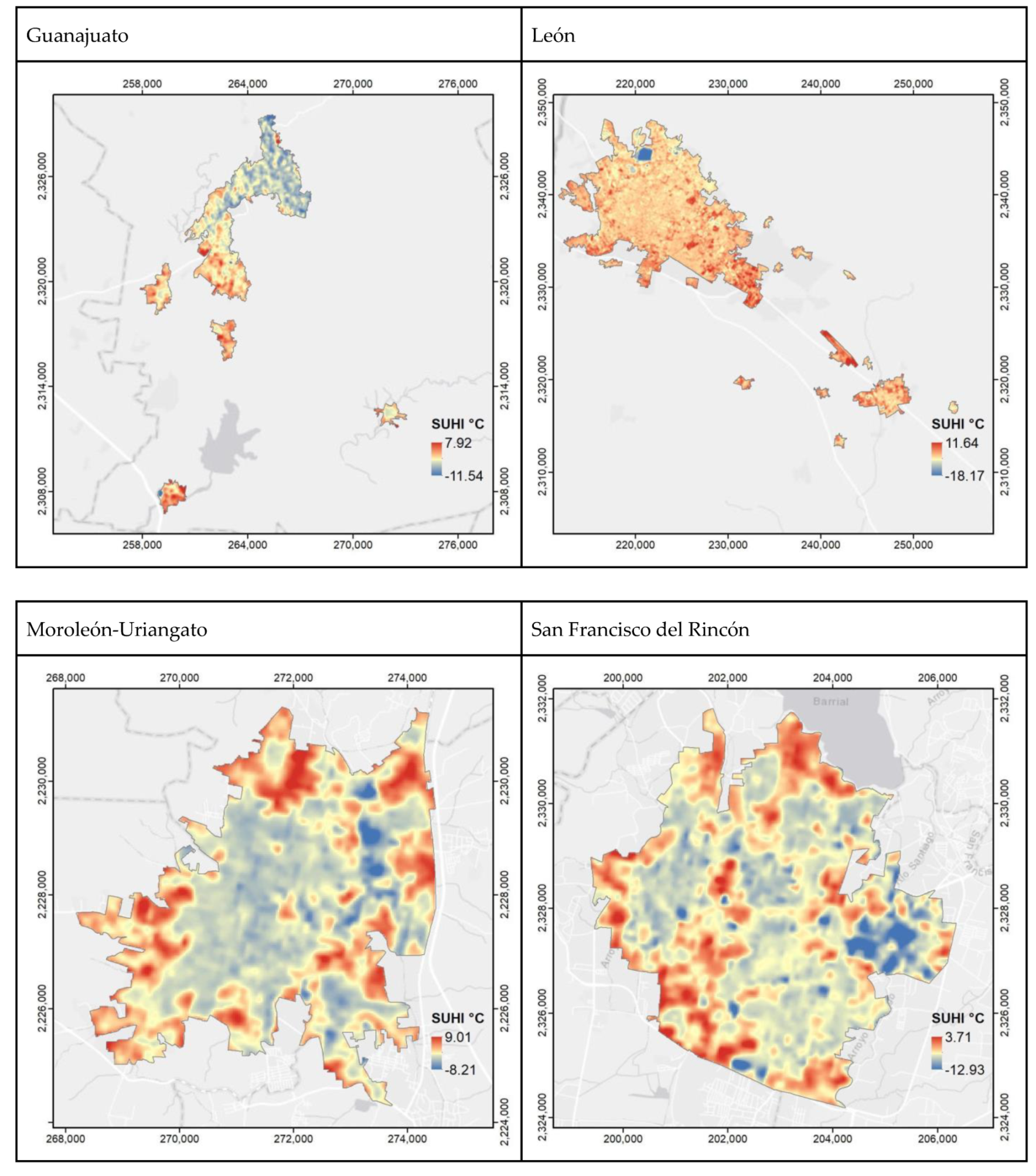
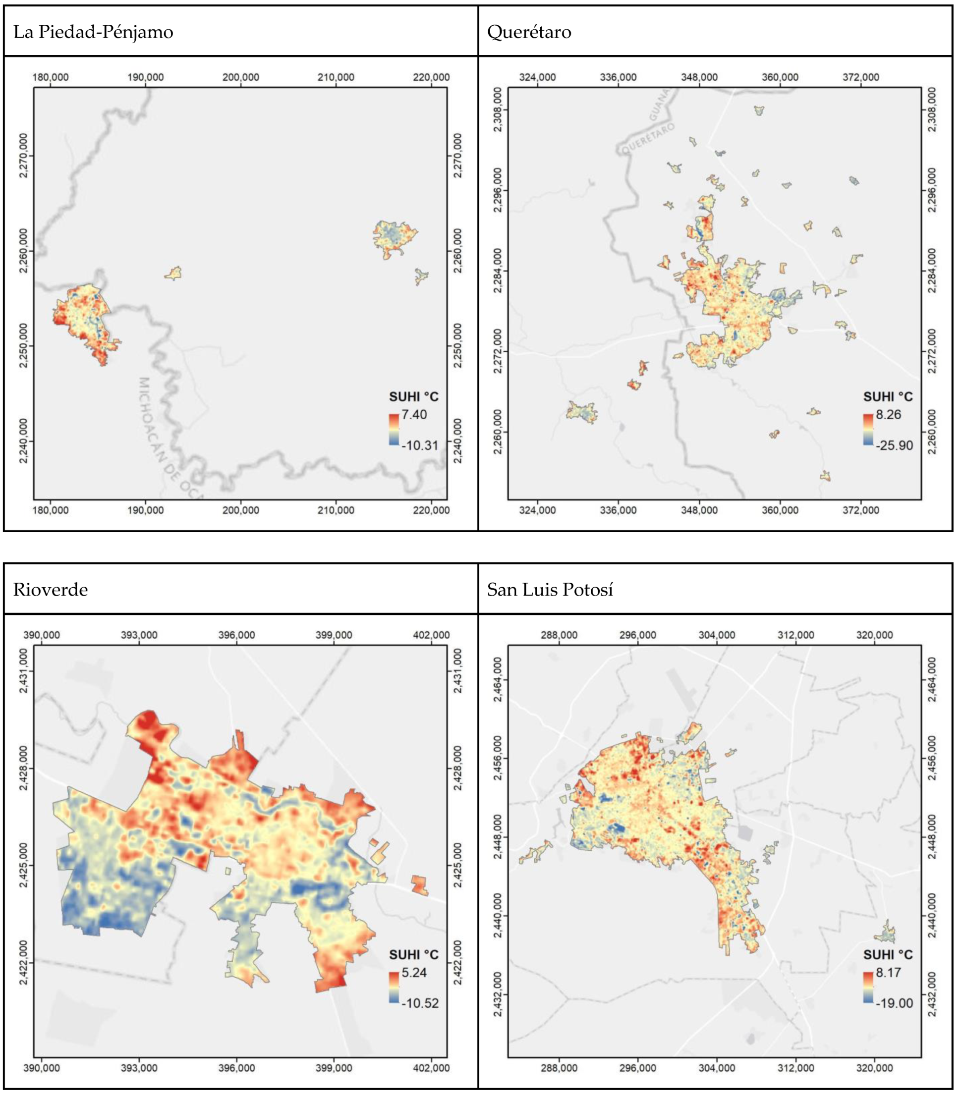
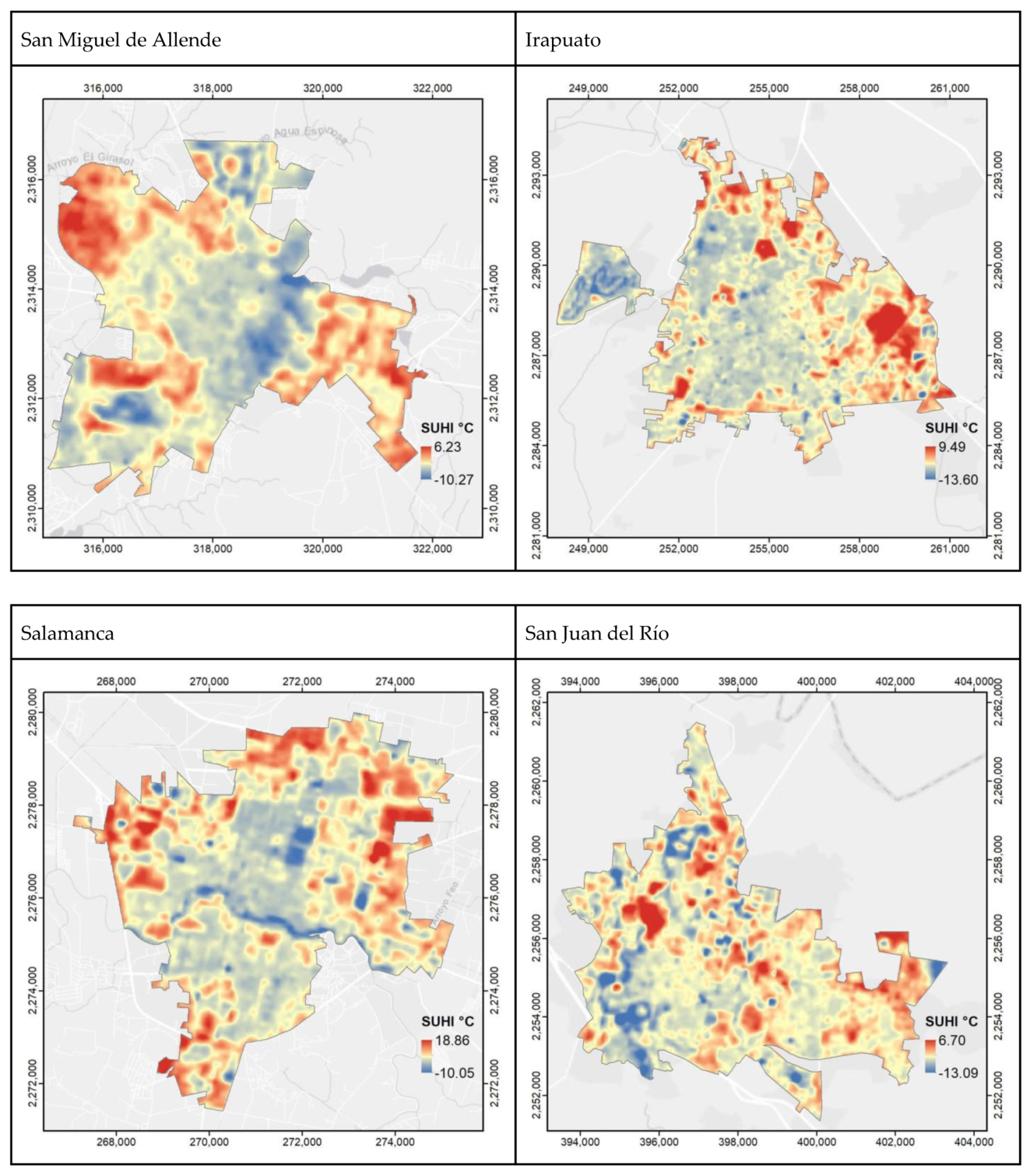
3.2. Daytime Landsat Surface Urban Heat Island 2020

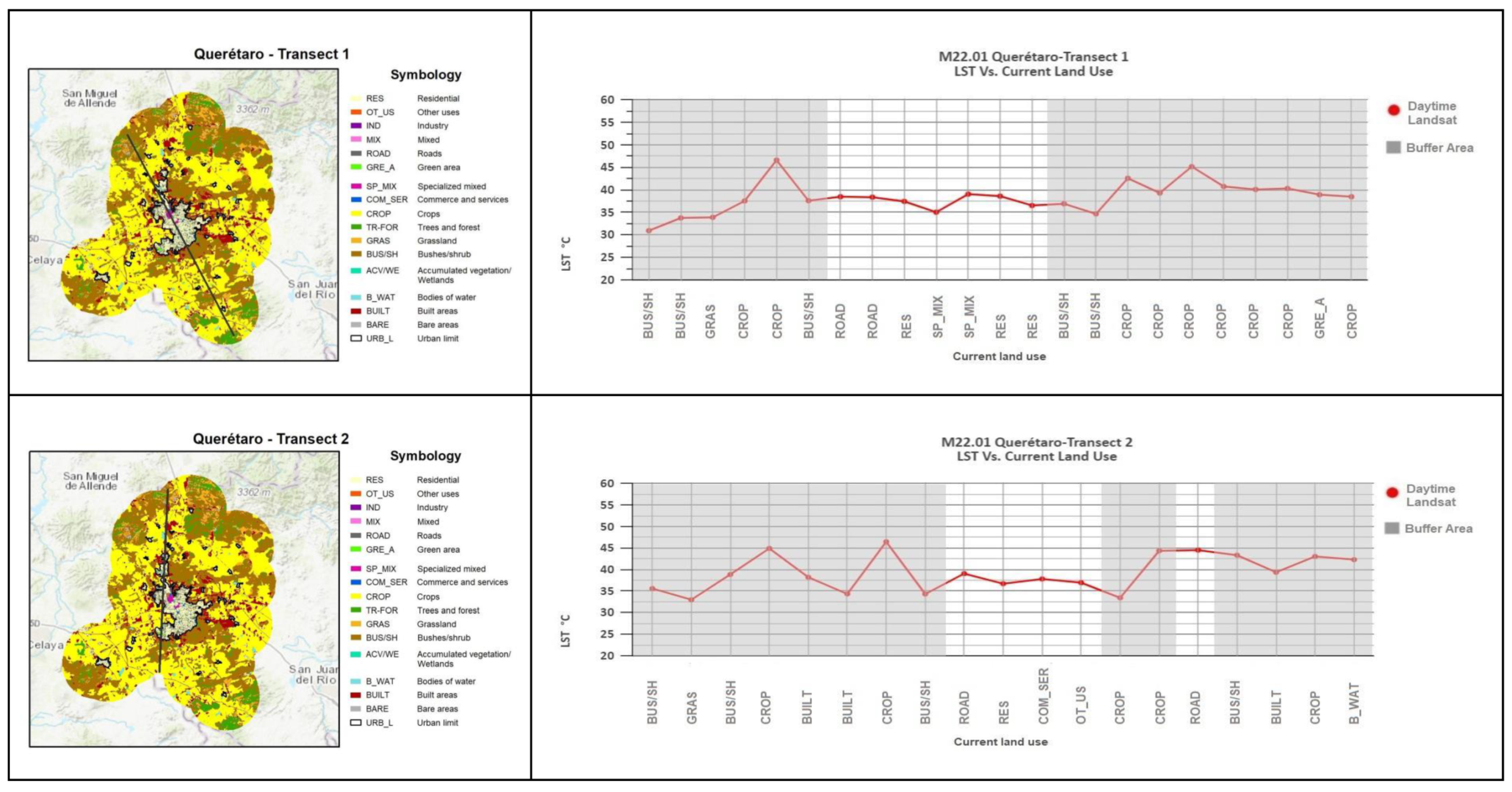
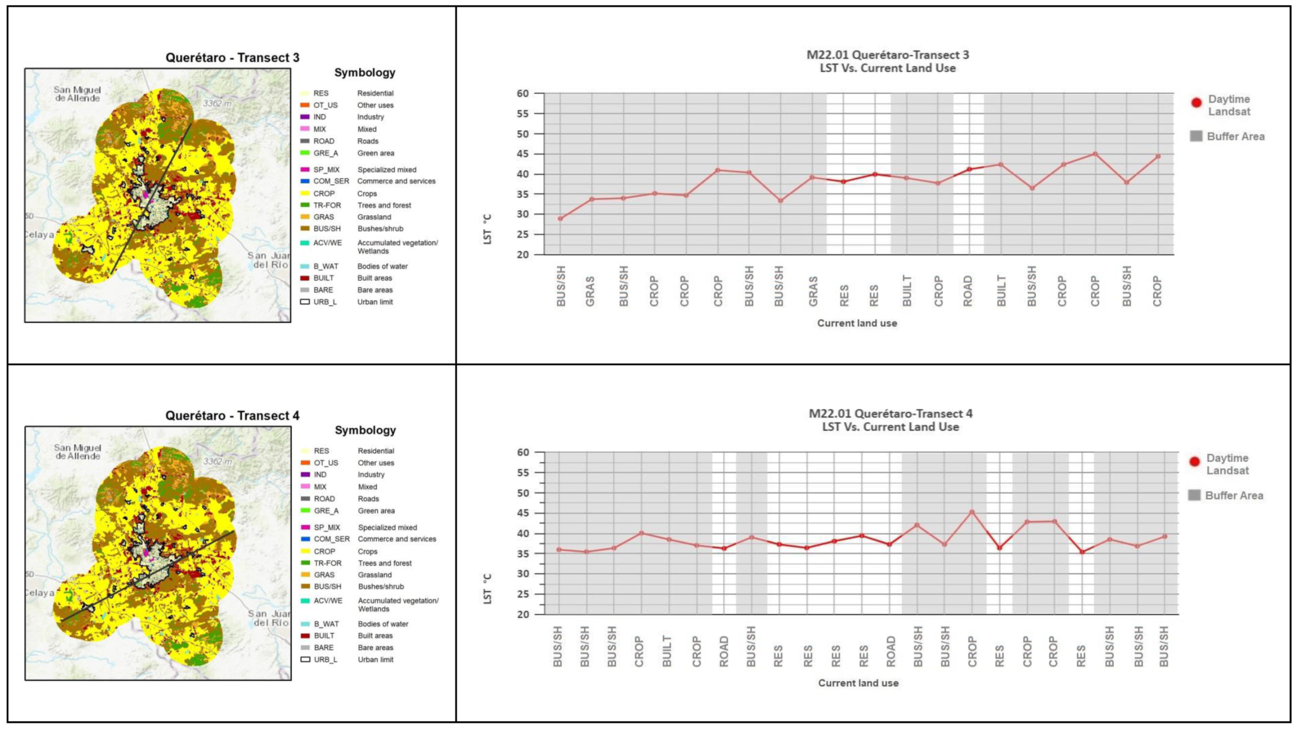
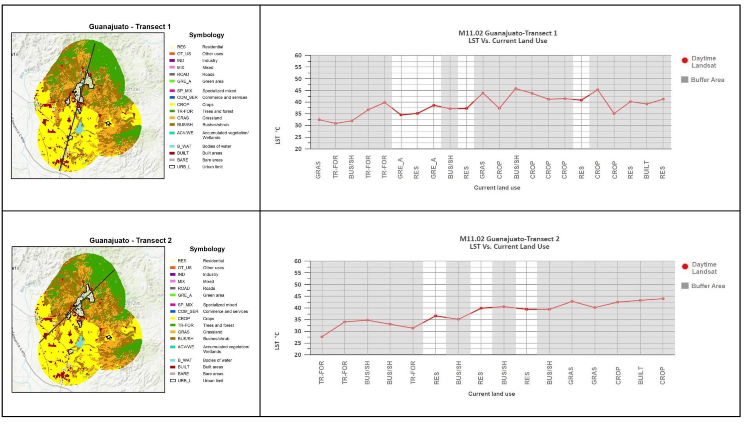
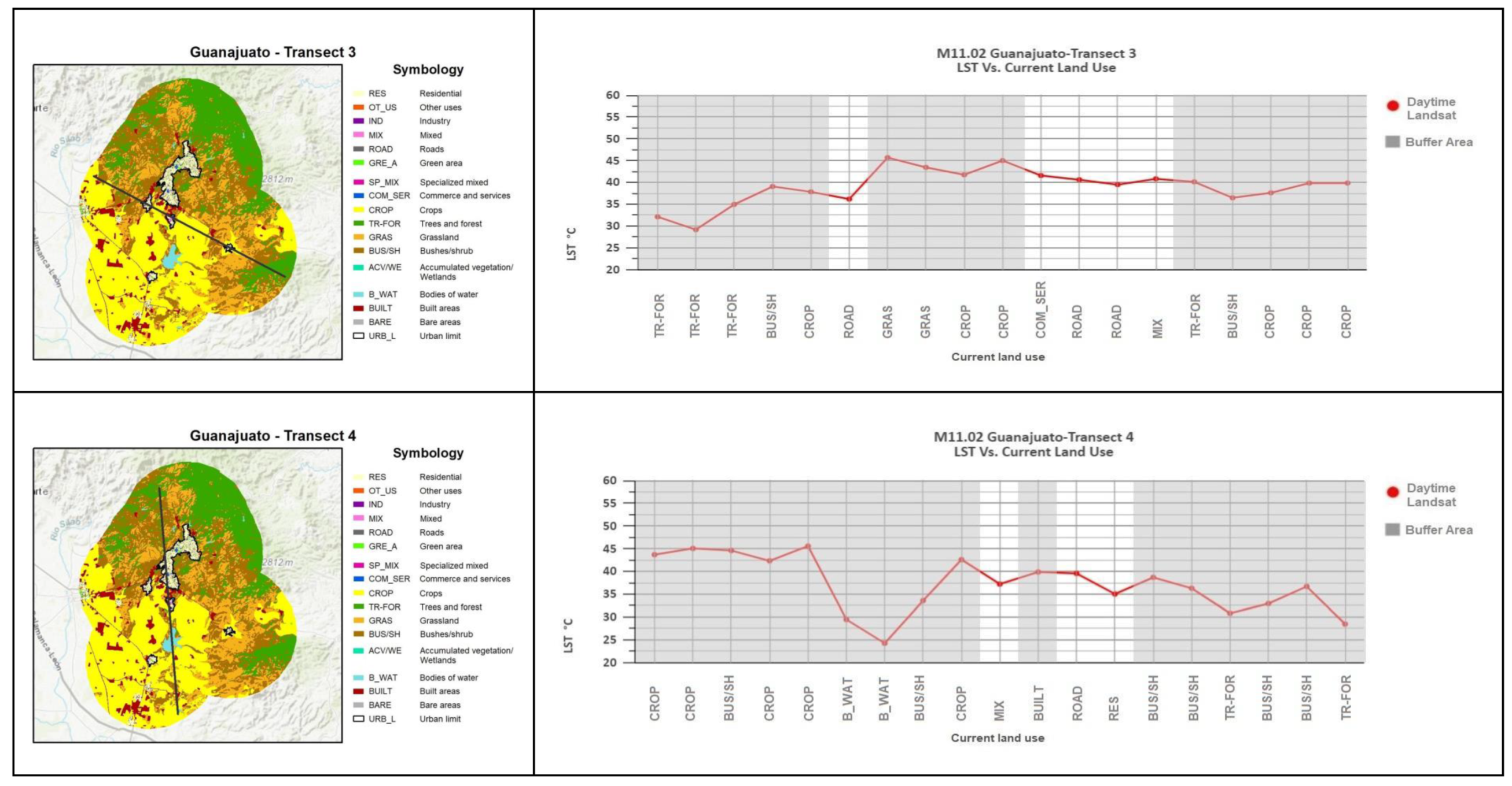
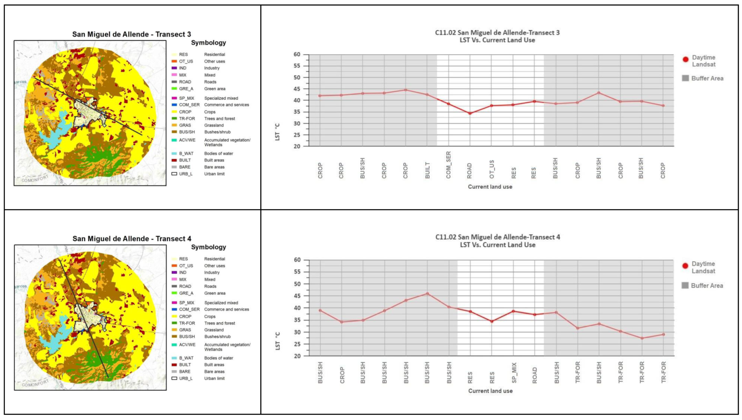
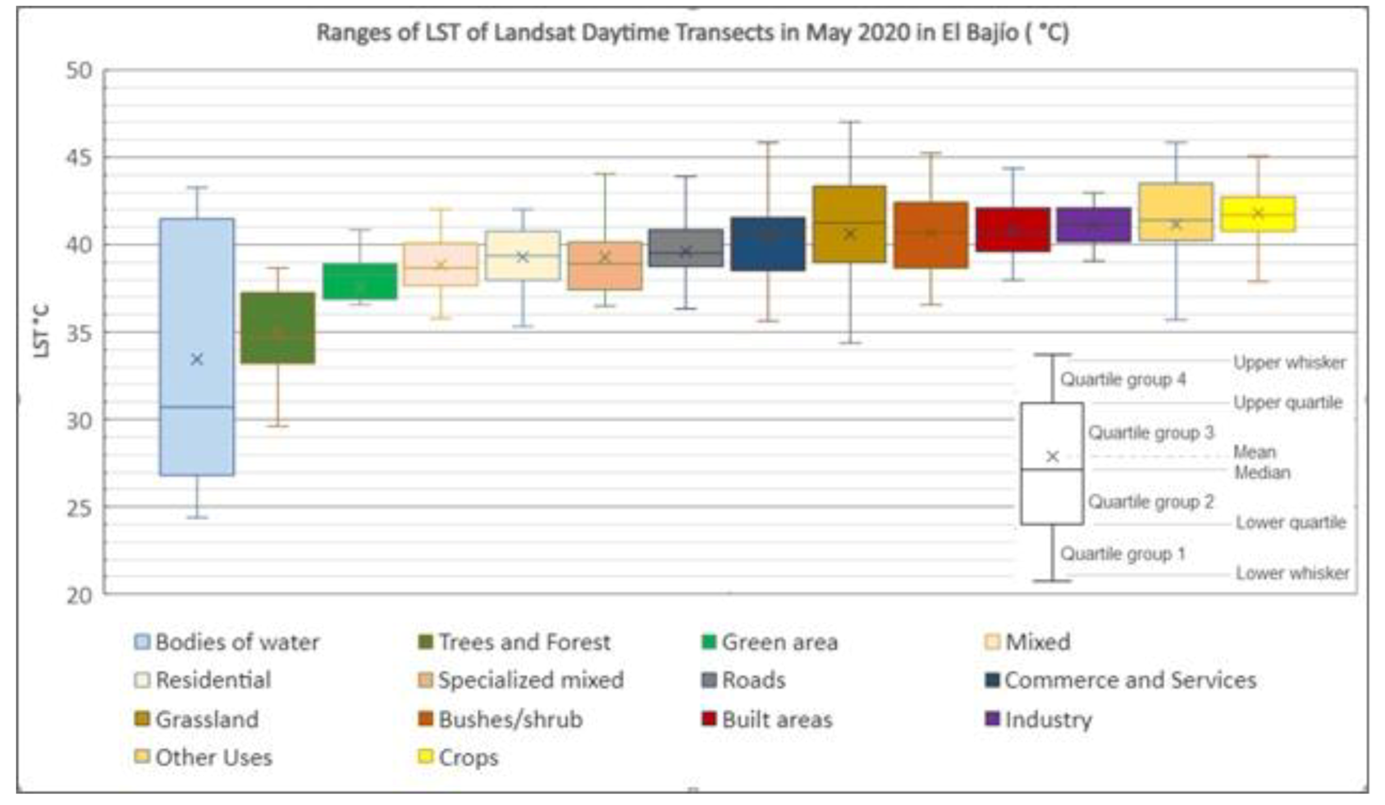
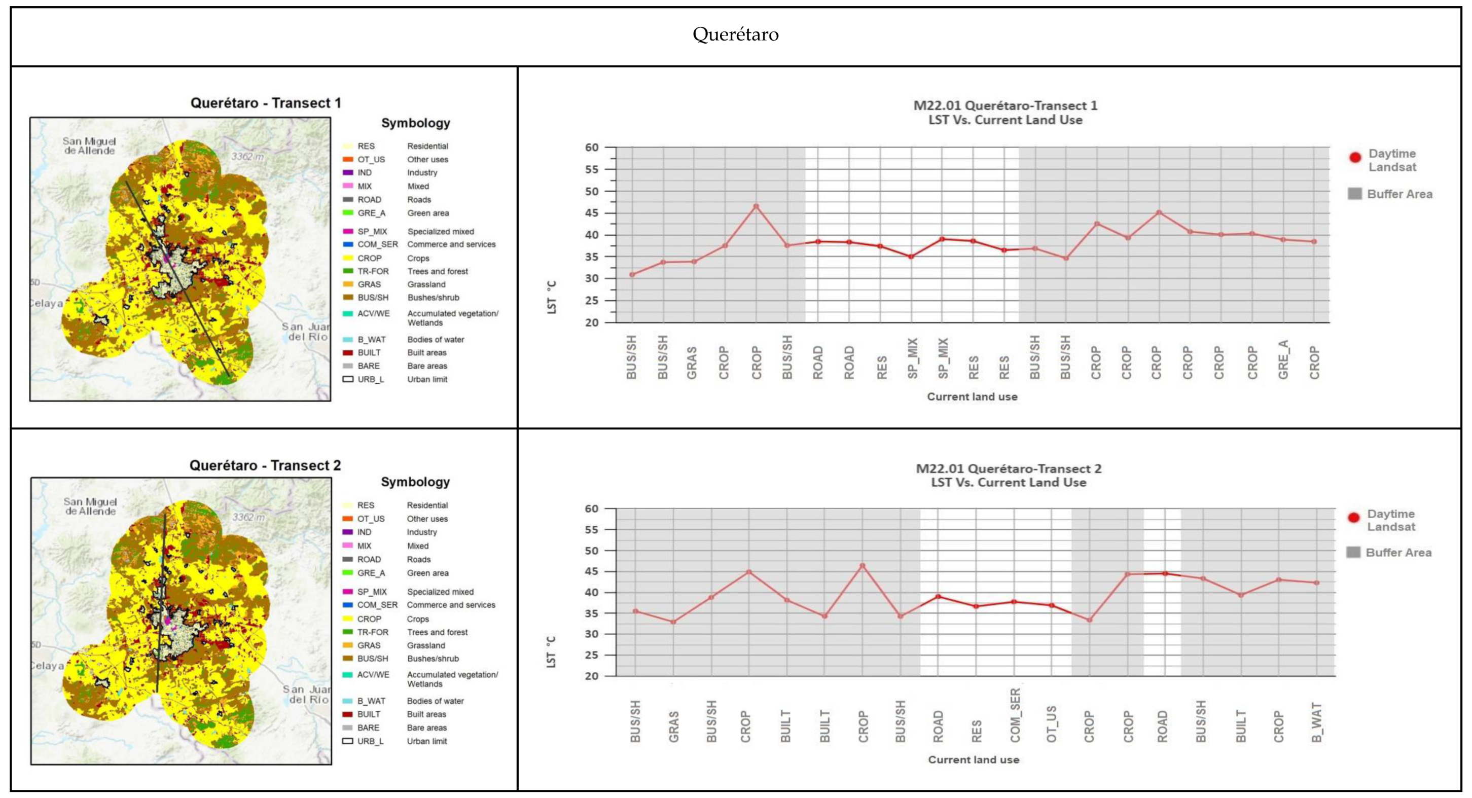
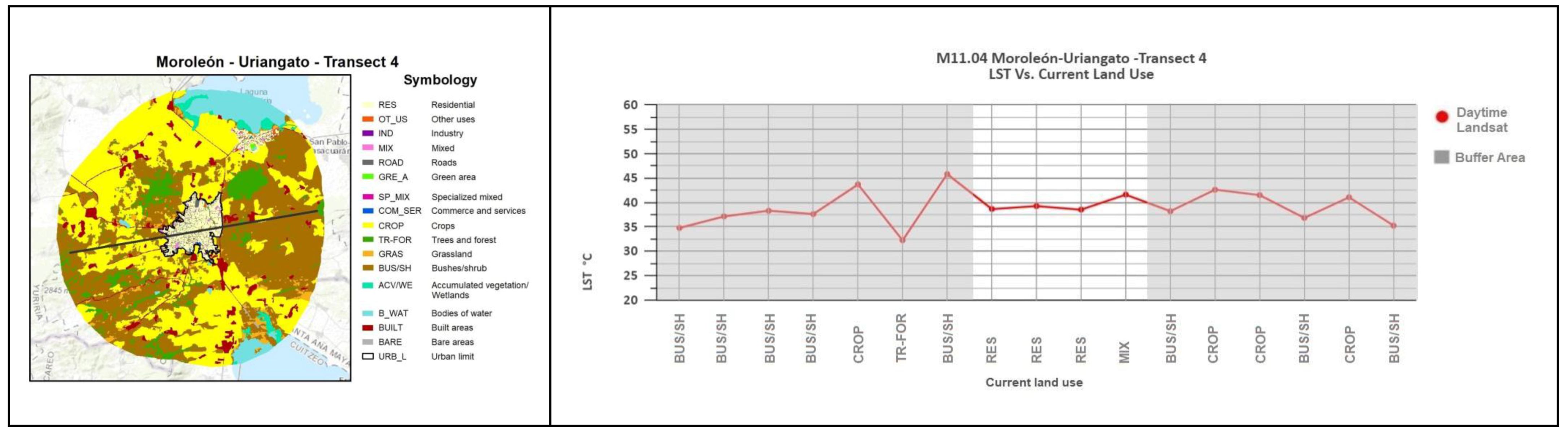
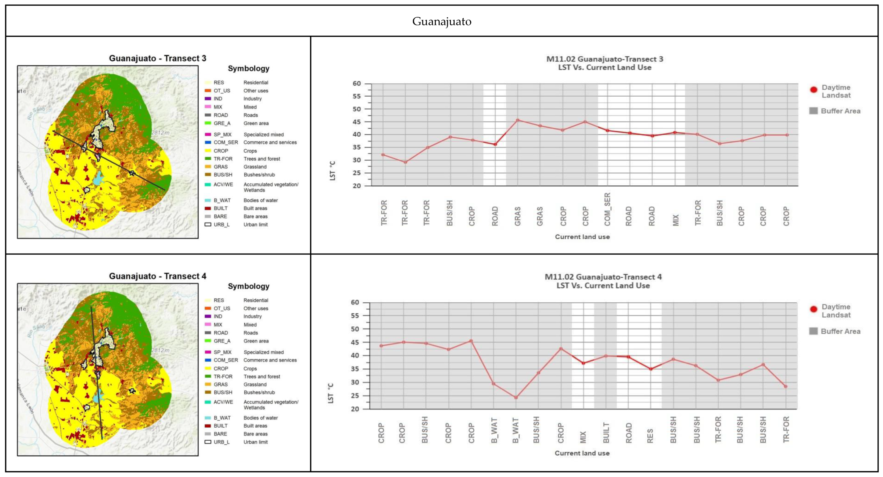
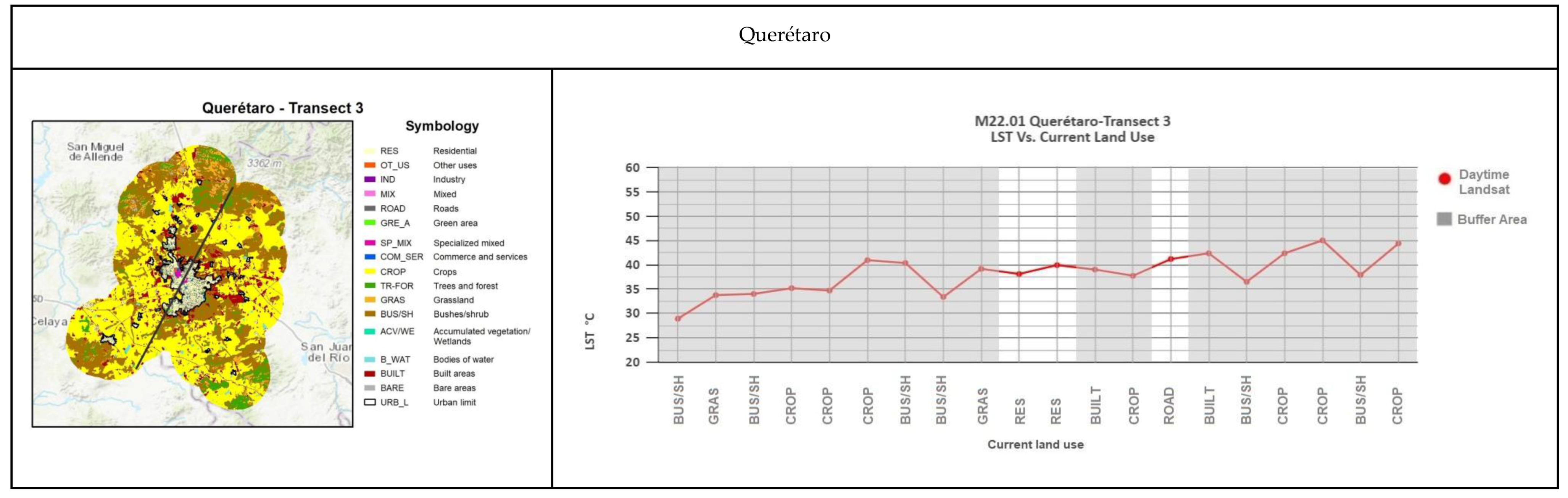
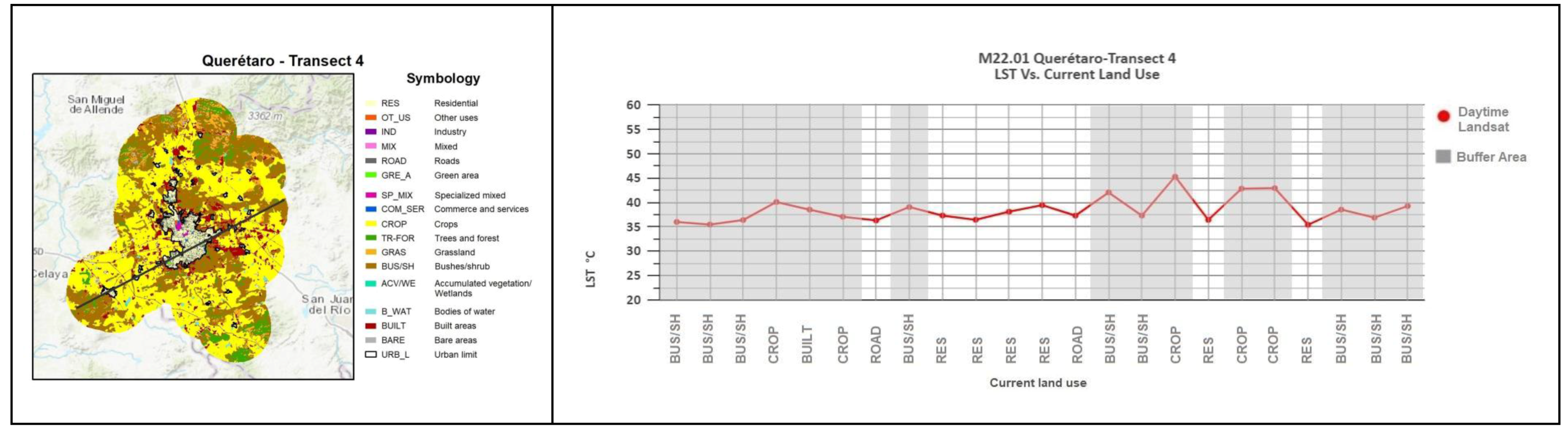
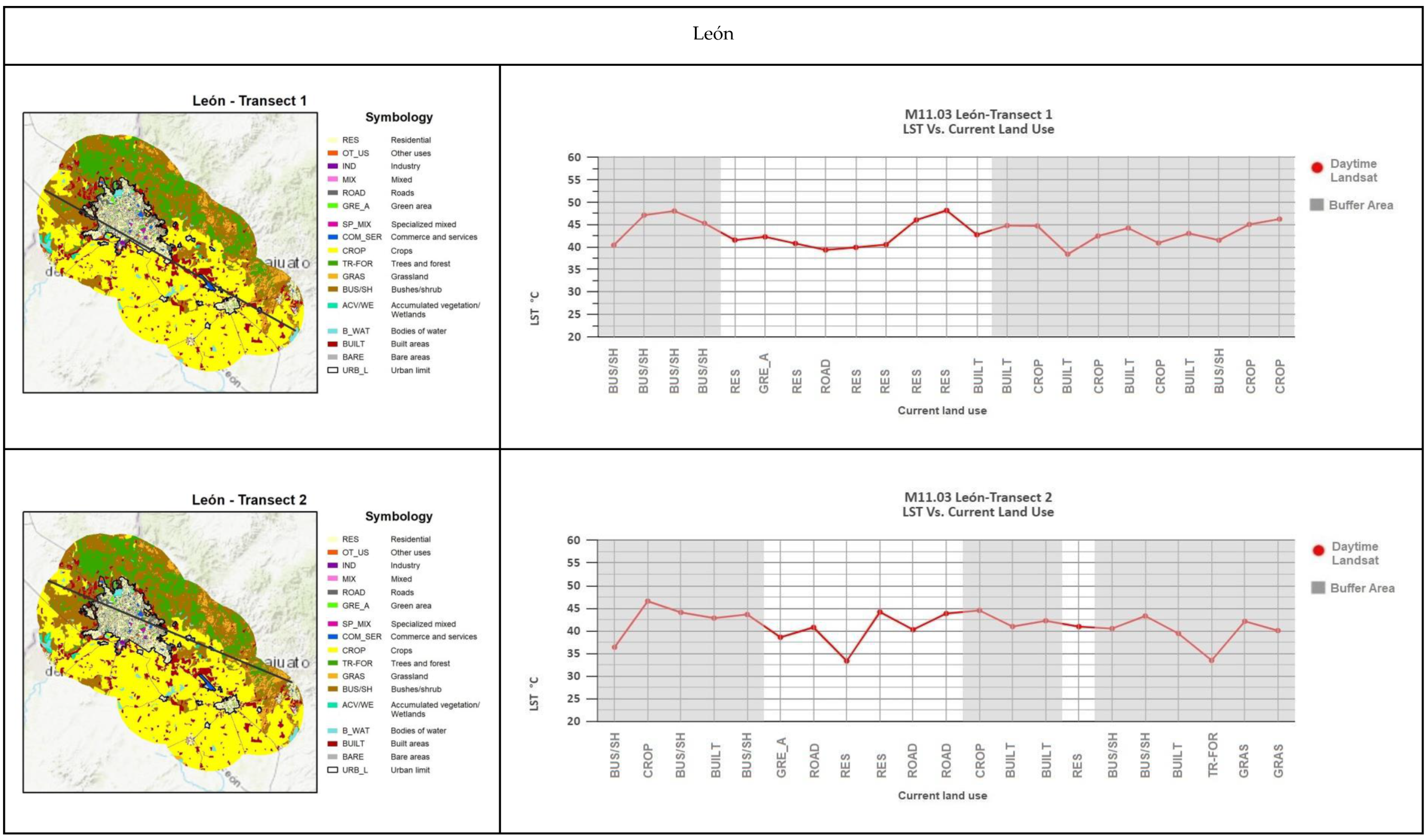
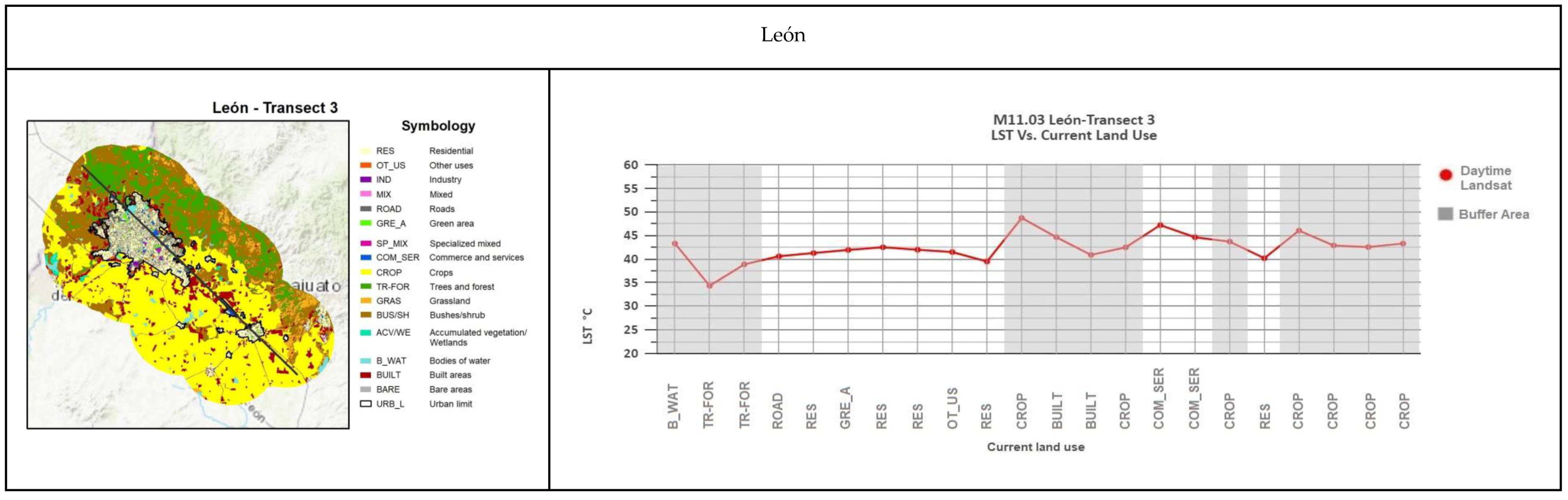
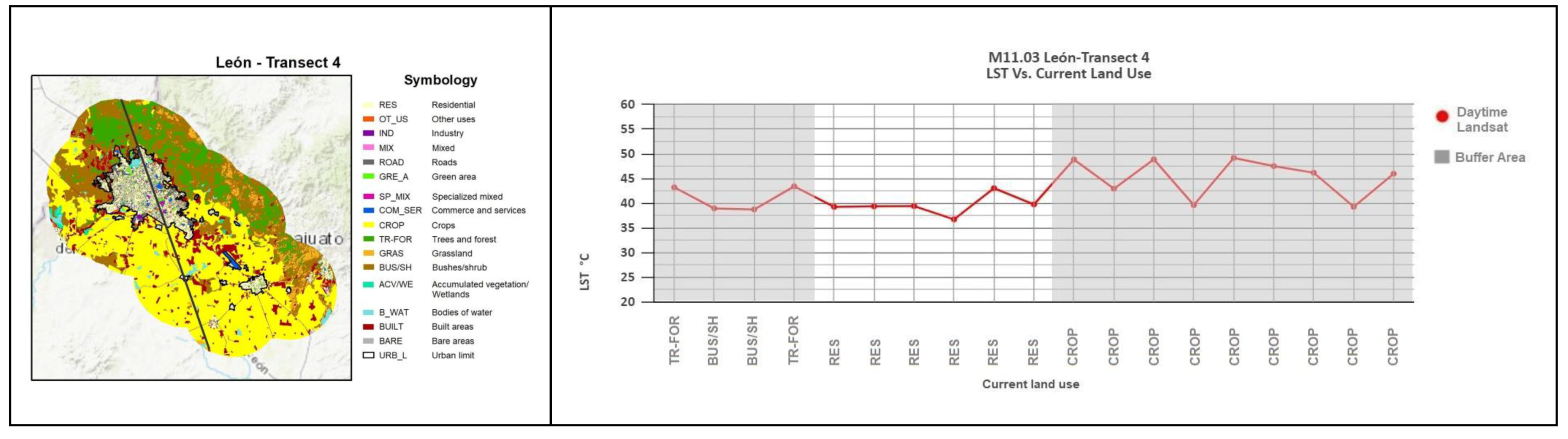
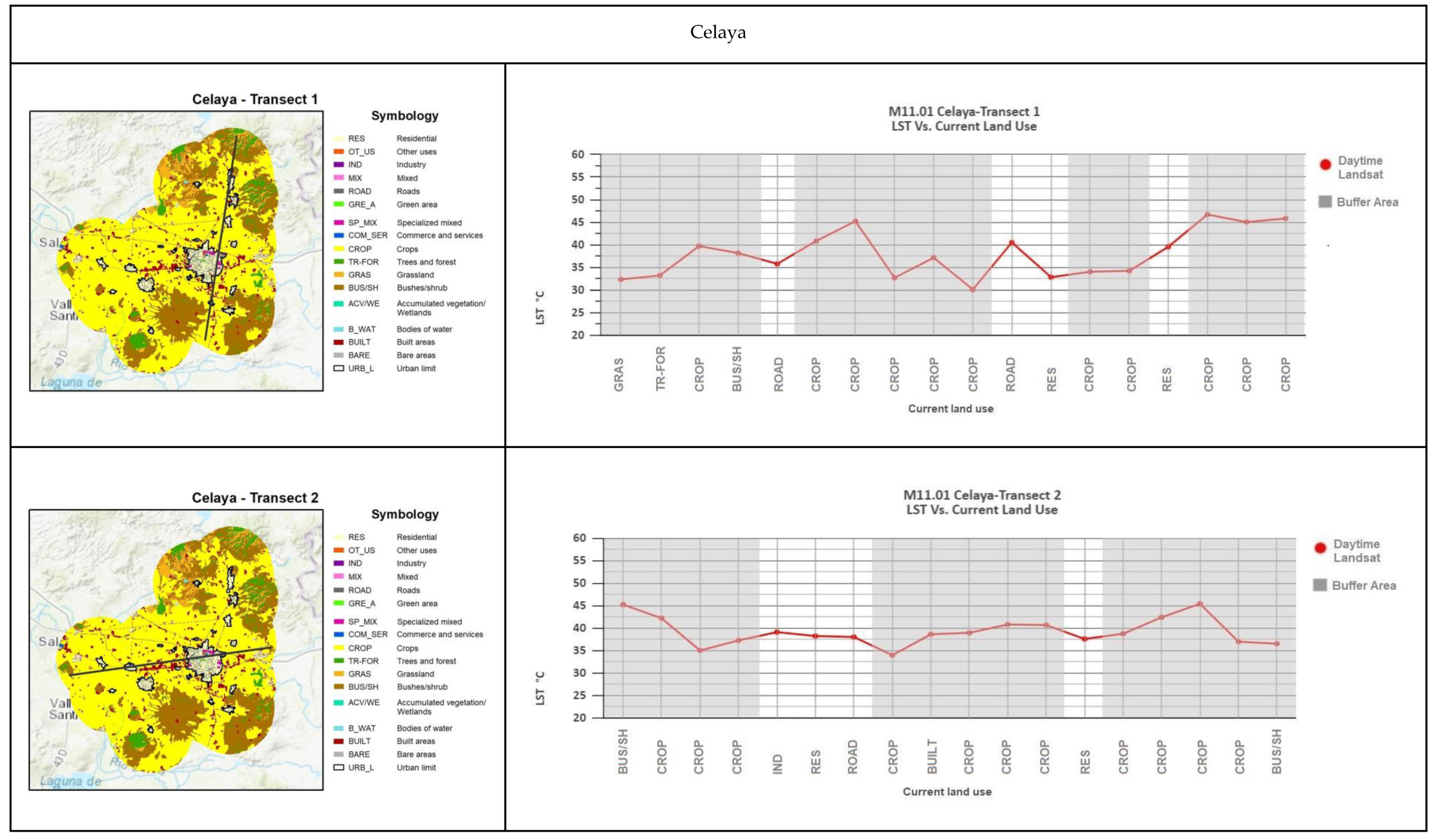
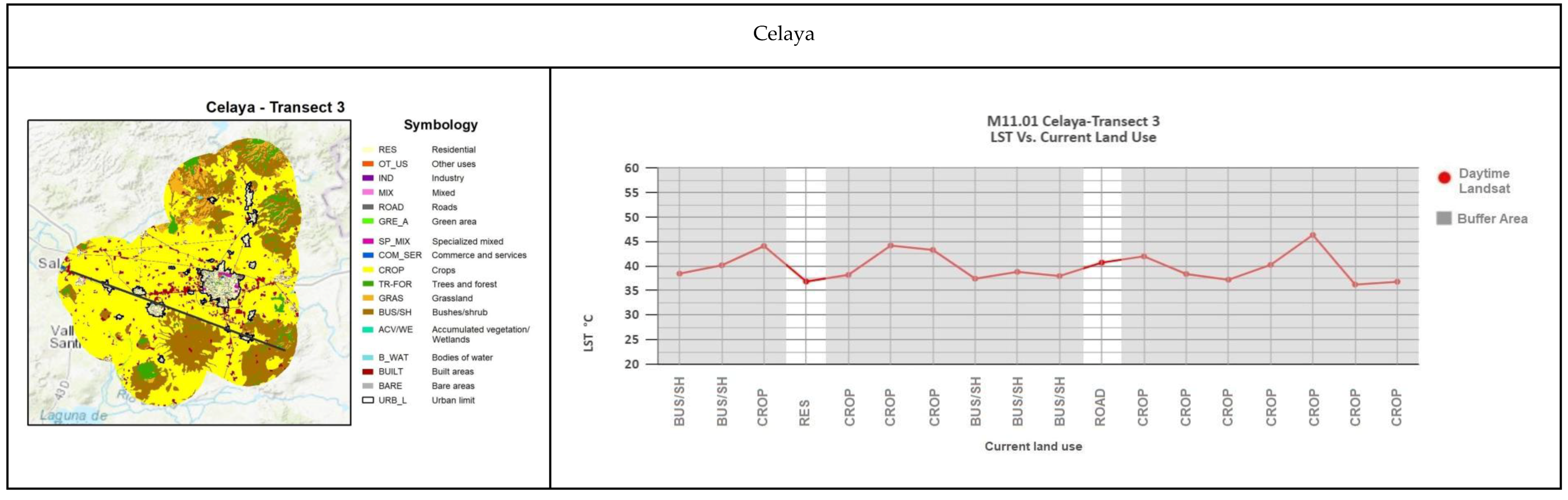
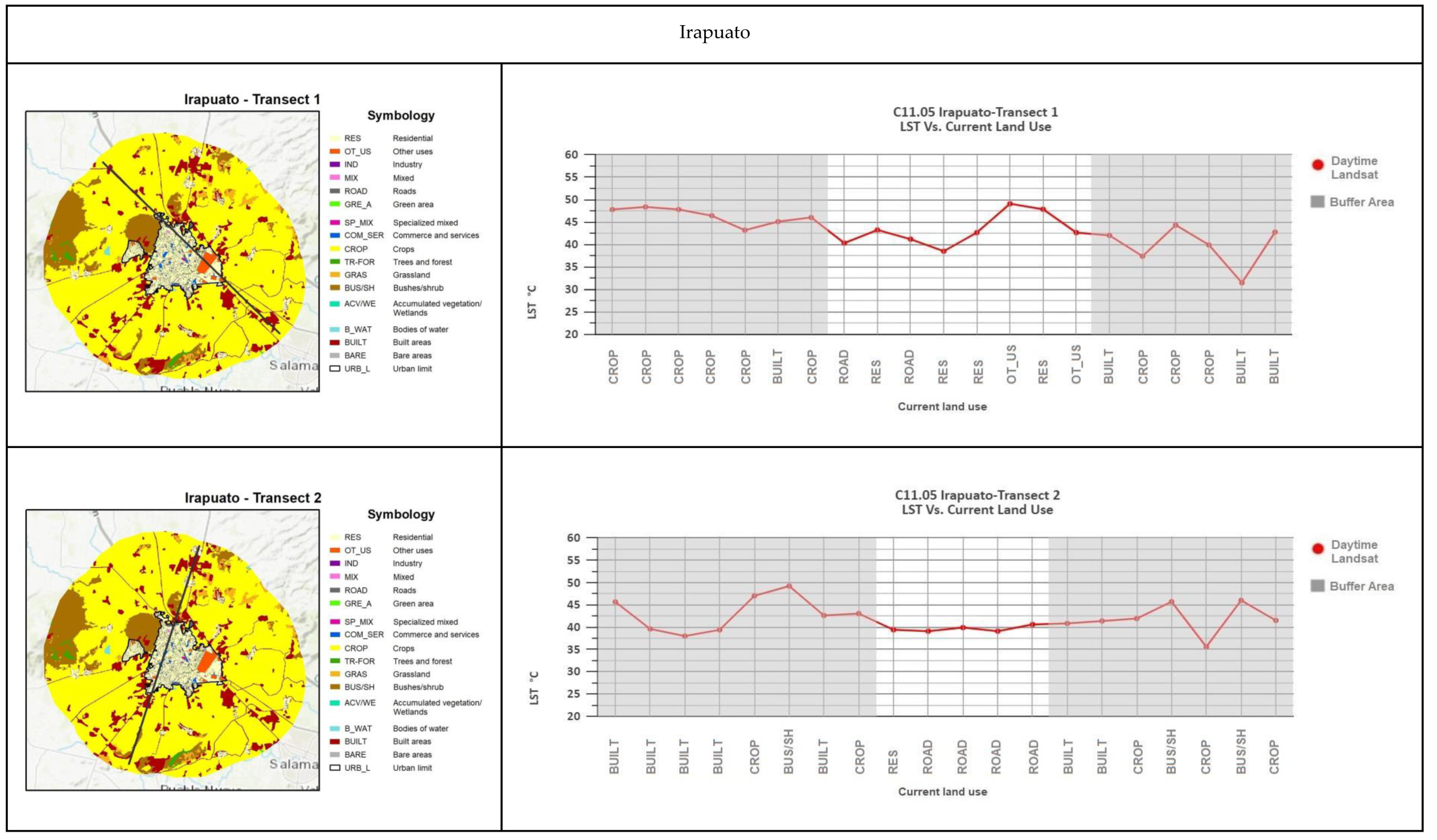
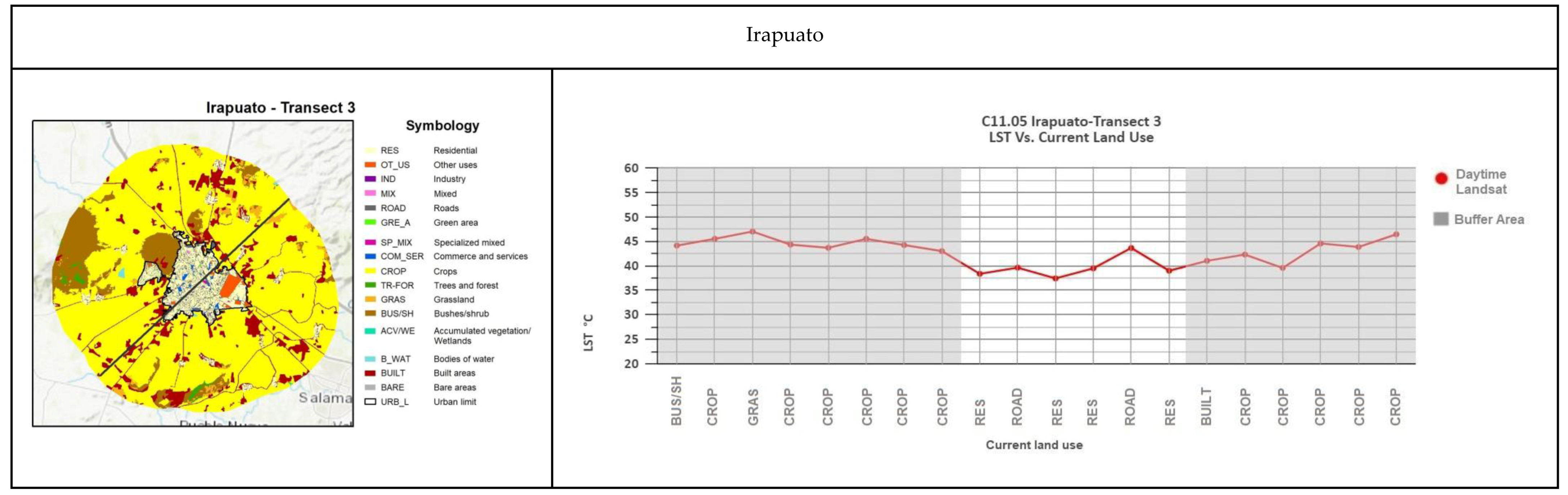
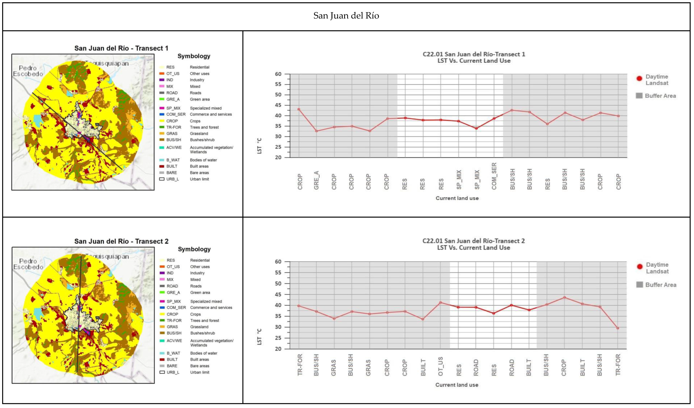
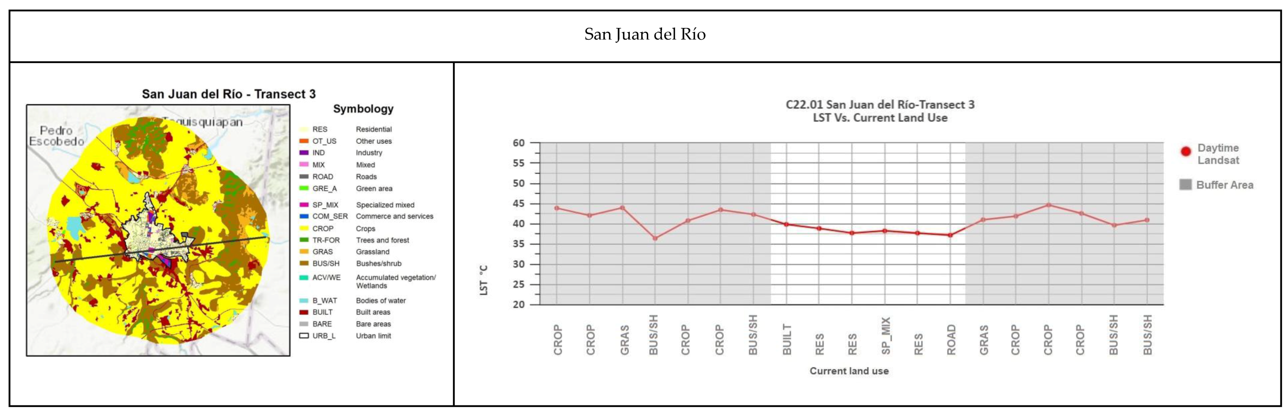
An analysis of the daytime SUHIs in Appendix A.2 shows that positive values indicate that LST is higher inside the urban area than outside in the buffer, while negative values indicate that the LST is higher in the buffer than in the urban area. As well as, in most of the El Bajío cities, the highest LST occurs within the city, creating a positive SUHI. The Landsat images show a minimum to maximum range of SUHIs from −18.1 to 18.9 °C, whereas for the fourteen cities, the average minimum is −3.4 °C and the average maximum of 2.5 °C, with an average difference of −1 °C. In other words, during the daytime in El Bajío in May 2020, the LST was 1 °C higher outside the urban area than inside. The behavior of SUHIs with Landsat in the El Bajío region can be seen in Figure 5 in their minimum, maximum, and average values by city. It is also possible to see the cities with negative SUHIs and the way some had extremely low minimums, as in the case of León with −18.1 °C or Querétaro with −16.8 °C, whereas Salamanca had a maximum of 18.9 °C.

The analysis of the Land Surface Temperature and the Surface Urban Heat Islands with daytime Landsat images shows that the LST not only varies according to the urban limit, but that due to its spatial resolution, it gives rise to exploration depending on the types of cover and soils inside and outside the urban limit. In this way, transect plotting is proposed to identify the LST according to the corresponding land cover or use and analyze its behavior.

3.3. Transects

We used transects of different distances to measure the SUHI effect in different classes of land cover and current land use. Four transects were built for each city in the study. Points were subsequently calculated every 3, 2, and 1.5 km according to the size of the city on the transects, and samples of the LST, land cover, and current land use were obtained; the results are shown in Appendix B.

In the largest cities with separation points of three kilometers, the transects show a temperature increase during the day in urban areas. The most temperate zones correspond to forests, followed by scrub and crops. In some cases, the transects tend to show SUHI and high LST points in urban areas. However, temperature anomalies are also found in certain crop areas, possibly due to the lack of bodies of water and the corridors of construction areas formed outside the urban limits.

Regarding Querétaro, the daytime images show the high surface temperatures associated with crop areas. There is a need to analyze the agricultural practices and the species planted in these areas. Moreover, it is essential to identify the materials used to build urban residential buildings due to the low temperatures they reflect. However, the behavior is as expected since the existing bodies of water do not significantly reduce the temperature of the surroundings, or at least this is not noticeable in the transects. Moreover, the SUHIs are concentrated in the western part of the city due to the concentration of manufacturing industries in that area (Figure 6).

Regarding the cities with separation points of two kilometers in their transects, as in the city of Guanajuato, the types of cover with low LST are trees and forests, bushes and scrub, and bodies of water. On the other hand, grasslands, crops, and residential land use increase LST. Due to the type of vegetation surrounding the city of Guanajuato, LST and SUHIs are more noticeable in the south since this area is predominantly under cultivation (Figure 7).

Finally, in the case of Rioverde, high surface temperatures are associated with bushes and scrub in cities with transects that have points every 1.5 km. In contrast, low temperatures are found in wooded areas. The urban area of Rioverde is a transition zone between the two, with no temperature anomalies. High LST values can be seen north of the city of Rioverde, whereas low temperatures are associated with the southwest.

The city of San Miguel de Allende has a significant percentage of water cover outside the urban area, demonstrating how bodies of water keep the surrounding areas of the urban area cool. Another factor in keeping the surrounding areas cool is the advantage of retaining a high percentage of the natural ecosystem around the urban area.

As shown in Figure 8, Transect 2 highlights the importance of water bodies in decreasing temperature and their function as heat sinks for neighboring areas. The SUHIs are therefore concentrated in the northwestern part of San Miguel de Allende; this region is the furthest from an extensive body of water and wooded areas.

The LST values summarized in the form of box plots in Figure 9 are especially representative of the land-cover categories that take up a high percentage of the cities in the El Bajío Industrial Corridor, Mexico. In this case, the crop areas and other land use related to exposed soils devoid of vegetation stand out as they present a higher LST than the green areas found within all the cities included in this study.

We associate the month of May with seasonal crops, which are of greater scope and profitability for many farmers in the country. In that case, there is a lower production of these foods since it also goes through a dry season, generating the presence of bare soils or with little vegetation, which consequently generates an increase in the LST. On the other hand, the dynamics within the cities are different. Many vegetation areas correspond to gardens, parks, and park areas, which maintain constant hydration by the neighborhoods or governmental maintenance programs, keeping the areas with continuous vegetation.

We assume that the crop zones correspond to the Panorama Agrolimentario 2020, as in the rest of the country, where grain corn, beans, sorghum, wheat, vegetables, and greens are the main crops [45]. On the other hand, the variety of techniques and conditions of cultivation must be considered, such as fallow, irrigation, rainfed, or/and greenhouse.

4. Discussion

Changes in land use are related to the context of anthropogenic climate change and global warming, meaning that their understanding and active management are increasingly important [46]. As noted in studies such as those by [47,48], the occurrence of Urban Surface Heat Islands depends on a range of factors, including large-scale and mesoscale climate conditions, microclimate, geographic location, the biophysical characteristics of the land surface, urban structure, population size, wind corridors, human lifestyle, and energy consumption. Apparently, zoning, as an urban planning tool, profoundly affects the physical characteristics of urban landscapes by imposing restrictions such as maximum building height and density, the extent of impervious surface and open space, and types of land use and activities. These variables, in turn, control surface energy exchange, surface and subsurface hydrology, micro- to mesoscale weather and climate systems, and other environmental processes [49].

The heat island effect is mainly due to a combination of factors, including the concentration of heat-absorbing surfaces, the lack of vegetation, and the presence of heat-generating sources. The view of profiles or transects in the different cities, therefore, enables one to observe the impact of these zonings on well-defined transects that show changes in land use and their association with changes in surface temperature, such as works in [50,51].

Within Mexican cities, [50] present a study of a city in northeastern Mexico. Characterized by large surfaces exposed to the sun, the study of this city shows a predominance of the city’s high temperatures due to pavements and buildings with scarce vegetation within the urban area. All measurements were obtained during the warm period in transects in the main roads of the urban layout, to which there is a significant presence of heavy industry, light industry, and large commercial corridors. In a similar study in Toluca city in central Mexico, [25] concluded that the high temperatures correspond to the area with the most extensive urban infrastructure located towards the city’s center. The lack of vegetation, the scarcity of bodies of water, multiple buildings, and construction with heat-absorbing materials, and a large concentration of vehicles characterize this area. Outside of cities, the heat island effect is generally less pronounced. The lower density of buildings and pavement and the presence of vegetation and agricultural activity can help dissipate heat and cool the air. However, fallow agricultural areas can also have the opposite effect and increase the urban heat island effect [52,53].

A study by Gough in 2020 [54] found that if fallow land is without proper management and the vegetation is allowed to dry out or die, the urban heat island effect can increase. In this case, the land can become a significant heat source rather than a heat sink and contribute to the urban heat island effect. Therefore, proper management and planning are crucial to mitigate potential adverse effects on the urban heat island [53,54,55].

Urban Heat Island studies are generally carried out mainly in two ways: first, by measuring UHI in air temperature using car transects and weather station networks; and second, by measuring UHI in surface temperature using remote sensing. The vast majority of climatological studies of UHI in Mexico have been carried out using in situ data, which have the advantage of high temporal resolution and an extensive data record; however, they have a poor spatial resolution and involve high costs due to measurement instruments acquisition and regular field trips. Whereas satellite thermal data, as in this case, have more excellent spatial coverage, allowing identification of UHI in a more versatile way, with the advantage of having more spatial and even temporal information at different coverage scales, such as local and regional.

Utilizing satellite data has become increasingly important for researchers and decision makers to understand the climatic effects of urbanization and, more importantly, how to contribute to more sustainable urban development. In such a way, the results of UHI studies between cities with different climatic and socioeconomic environments, such as ours, use data that allow for the identification of areas vulnerable to UHI, which, in turn, can be related to other fields of study, such as health, by identifying diseases that have developed in specific areas of the cities or sectors of the population derived from UHI. This research work is a precedent for other studies in the methodology employed and how the results are presented in terms of comparing the same region in different temporalities or regions with similar land-cover characteristics. In addition, it can serve as theoretical support material to forecast future behavior and propose measures that will allow, if not diminish, the effect of the UHI to be controlled or redistributed through implementing public policy strategies.

5. Conclusions

Through the incorporation of thermal profiles, the proposed methodology makes it possible to identify the land uses that intensify the LST, providing detailed information on the variation with distinct types of land cover. It also details the importance, for example, of green and blue areas, as well as crop areas within urban environments. In the present study, we used box plots to show the distribution of LST transects of different distances in different land use types. We analyzed the urban heat island effect in cities of the El Bajío Industrial Corridor in Mexico.

With respect to the case study, the peri-urban expansion that increases the use of urban land in a gradient ranging from natural ecosystems to crop areas and built areas (such as buildings, industries, housing, and roads), significantly affects the temperature change in cities.

The characteristics of the cities in El Bajío that most intensify the effect of the SUHIs have greater urban conglomeration; in other words, the built areas are not scattered. Other characteristics include having limited vegetation or green areas and a sizable industrial or mixed area, with few or no bodies of water, which have been seen to operate as temperature regulators. Furthermore, located around urban areas, crops such as vegetables, red fruits, corn, wheat, and sorghum that use fallow as part of agricultural practices minimize natural areas and directly contribute to the increase in temperature in the SUHI. This warrants a more specific study to identify the species causing this to find a way to mitigate this effect.

Finally, processing the images with the tools described proved helpful in automating the process. Moreover, since the tools used in this study are affordable for everyone, and given that the software is free and open source, the proposed procedure can be widely used in other cities.

References

1. Rao, P.K. Remote sensing of urban “heat islands” from an environmental satellite. AMER Meteorol. Soc. 1972, 53, 647–648. [Google Scholar]
2. Oleson, K.W.; Bonan, G.B.; Feddema, J. Effects of white roofs on urban temperature in a global climate model. Geophys. Res. Lett. 2010, 37. [Google Scholar] [CrossRef] [Green Version]
3. Fuentes Pérez, C.A. Islas de Calor Urbano en Tampico, México: Impacto del microclima a la calidad del hábitat. Nova Sci. 2015, 7, 495–515. [Google Scholar] [CrossRef] [Green Version]
4. Morales Méndez, C.C.; Madrigal Uribe, D.; González Becerril, L.A. Isla de calor en Toluca, México. CIENCIA ergo-sum, Revista Científica Multidisciplinaria de Prospectiva. Atmósfera 2007, 14, 307–316. [Google Scholar] [CrossRef]
5. Roth, M. Effects of cities on local climates. In Proceedings of the Workshop of Institute for Global Environment Studies/Asia-Pacific Network (IGES/APN) Mega-city Project, Kitakyushu, Japan, 23–24 January 2002. [Google Scholar]
6. Oke, T.R. The urban energy balance. Prog. Phys. Geogr. 1988, 12, 471–508. [Google Scholar] [CrossRef]
7. Kalnay, E.; Cai, M. Impact of urbanization and land-use change on climate. Nature 2003, 423, 528–531. [Google Scholar] [CrossRef]
8. Zhou, L.M.; Dickinson, R.E.; Tian, Y.H.; Fang, J.Y.; Li, Q.X.; Kaufmann, R.K.; Myneni, R.B. Evidence for a significant urbanization effect on climate in China. Proc. Natl. Acad. Sci. USA 2004, 101, 9540–9544. [Google Scholar] [CrossRef] [Green Version]
9. Jones, P.D.; Lister, D.H.; Li, Q. Urbanization effects in large scale temperature records, with an emphasis on China. J. Geophys. Res. Atmos. 2008, 113. [Google Scholar] [CrossRef]
10. Parker, D.E. Urban heat island effects on estimates of observed climate change. WIREs Clim. Chang. 2010, 1, 123–133. [Google Scholar] [CrossRef]
11. Fujibe, F. Detection of urban warming in recent temperature trends in Japan. Int. J. Climatol Q. J. R. Meteorol. Soc. 2009, 29, 1811–1822. [Google Scholar] [CrossRef]
12. Stone, B. Urban and rural temperature trends in proximity to large US cities: 1951–2000. Int. J. Climatol Q. J. R. Meteorol. Soc. 2007, 27, 1801–1807. [Google Scholar] [CrossRef]
13. Grimmond, C.S.B.; Blackett, M.; Best, M.J.; Barlow, J.; Baik, J.-J.; Belcher, S.E.; Bohnenstengel, S.I.; Calmet, I.; Chen, F.; Dandou, A.; et al. The international urban energy balance models comparison project: First results from phase 1. J. Appl. Meteorol. Climatol. 2010, 49, 1268–1292. [Google Scholar] [CrossRef]
14. Sabrin, S.; Karimi, M.; Nazari, R. Developing Vulnerability Index to Quantify Urban Heat Islands Effects Coupled with Air Pollution: A Case Study of Camden, NJ. ISPRS Int. J. Geo-Information 2020, 9, 349. [Google Scholar] [CrossRef]
15. Nichol, J.E. High-resolution surface temperature patterns related to urban morphology in a tropical city: A satellite-based study. J. Appl. Meteorol. Climatol. 1996, 35, 135–146. [Google Scholar] [CrossRef]
16. Streutker, D.R. A remote sensing study of the urban heat island of Houston, Texas. Int. J. Remote Sens. 2002, 23, 2595–2608. [Google Scholar] [CrossRef]
17. Ángel, L.; Ramírez, A.; Domínguez, E. Isla de calor y cambios espacio-temporales de la temperatura en la ciudad de Bogotá. Rev. Acad. Colomb. Cienc. 2010, 34, 173–183. [Google Scholar]
18. Nichol, J.; Wong, W.S. Modeling urban environmental quality in a tropical city. Landsc. Urban. Plan. 2005, 73, 49–58. [Google Scholar] [CrossRef]
19. Owen, T.W.; Carlson, T.N.; Gillies, R.R. An assessment of satellite remotely-sensed land cover parameters in quantitatively describing the climatic effect of urbanization. Int. J. Remote Sens. 1998, 19, 1663–1681. [Google Scholar] [CrossRef] [Green Version]
20. Voogt, J.A.; Oke, T.R. Thermal remote sensing of urban climates. Remote Sens. Environ. 2003, 86, 370–384. [Google Scholar] [CrossRef]
21. Roth, M.; Oke, T.R.; Emery, W.J. Satellite-derived urban heat islands from three coastal cities and the utilization of such data in urban climatology. Int. J. Remote Sens. 1989, 10, 1699–1720. [Google Scholar] [CrossRef]
22. Imhoff, M.L.; Zhang, P.; Wolfe, R.E.; Bounoua, L. Remote sensing of the urban heat island effect across biomes in the continental USA. Remote Sens. Environ. 2010, 114, 504–513. [Google Scholar] [CrossRef] [Green Version]
23. Jáuregui, E. Heat island development in Mexico City. Atmos. Environ. 1997, 31, 3821–3831. [Google Scholar] [CrossRef]
24. Barradas, V.L. La Isla de Calor Urbana y la Vegetación Arbórea; Oikos Publicación del Instituto de Ecología, UNAM: Ciudad de México, México, 2016; pp. 1–4. [Google Scholar]
25. Romero Dávila, S.; Morales Méndez, C.C.; Némiga, X.A. Identificación de las islas de calor de verano e invierno en la ciudad de Toluca, México. Rev. Climatol. 2011, 11. [Google Scholar]
26. Soto Diaz, A.B.; Pérez Ruiz, E.R. Uso de Percepción Remota y Sistemas de Información Geográfica Para la Determinación de ISLAS de Calor Urbano en Ciudad Juárez, Chihuahua. Memorias de Resúmenes en Extenso SELPER-XXI-México-UACJ-2015. 2015. Available online: https://www.uacj.mx/CGTI/CDTE/JPM/Documents/SELPER/assets/m016.pdf (accessed on 28 December 2022).
27. CONAPO, SEDESOL, SEGOB. Catálogo Sistema Urbano Nacional 2018. México, Consejo Nacional de Población (CONAPO). Secretaría de Desarrollo Social (SEDESOL). Secretaría de Gobernación (SEGOB). 2018. Available online: http://www.gob.mx/cms/uploads/attachment/file/400771/SUN_2018.pdf (accessed on 28 December 2022).
28. Marco Geoestadístico, Instituto Nacional de Estadística y Geografía (INEGI 2017). Available online: https://www.inegi.org.mx/app/biblioteca/ficha.html?upc=889463142683 (accessed on 5 December 2021).
29. Zhou, D.; Xiao, J.; Bonafoni, S.; Berger, C.; Deilami, K.; Zhou, Y.; Sobrino, J.A. Satellite remote sensing of surface urban heat islands: Progress, challenges, and perspectives. Remote Sens. 2019, 11, 48. [Google Scholar] [CrossRef] [Green Version]
30. GlobeLand30: Global Geo-Information Public Product. Available online: http://www.globallandcover.com/ (accessed on 5 December 2021).
31. Resúmenes Mensuales de Temperaturas y Lluvia. Comisión Nacional del Agua (CONAGUA). Available online: https://smn.conagua.gob.mx/es/climatologia/temperaturas-y-lluvias/resumenes-mensuales-de-temperaturas-y-lluvias (accessed on 12 January 2021).
32. Acharya, T.D.; Yang, I. Exploring Landsat 8. IJIEASR 2015, 4, 4–10. [Google Scholar]
33. Ihlen, V. Landsat 8 (L8) Data Users Handbook; US Geological Survey: Sioux Falls, SD, USA, 2019. [Google Scholar]
34. Sobrino, J.; Raissouni, N.; Li, Z.-L. A comparative study of land surface emissivity retrieval from NOAA data. Remote Sens. Environ. 2001, 75, 256–266. [Google Scholar] [CrossRef]
35. Valor, E.; Caselles, V. Mapping land surface emissivity from NDVI: Application to European, African, and South American areas. Remote Sens. Environ. 1996, 57, 167–184. [Google Scholar] [CrossRef]
36. Van de Griend, A.; OWE, M. On the relationship between thermal emissivity and the Normalized Difference Vegetation Index for natural surfaces. Int. J. Remote Sens. 1993, 14, 1119–1131. [Google Scholar] [CrossRef]
37. Sobrino, J.A.; Jiménez-Muñoz, J.C.; Sòria, G.; Romaguera, M.; Guanter, L.; Moreno, J.; Martínez, P. Land surface emissivity retrieval from different VNIR and TIR sensors. IEEE Trans. Geosci. Remote Sens. 2008, 46, 316–327. [Google Scholar] [CrossRef]
38. Rouse, J. Monitoring the vernal advancement of retrogradation of natural vegetation. NASA/GSFC Type III Final. Rep. Greenbelt MD 1974, 371. [Google Scholar]
39. Carlson, T.N.; Ripley, D.A. On the relation between NDVI, fractional vegetation cover, and leaf area index. Remote Sens. Environ. 1997, 62, 241–252. [Google Scholar] [CrossRef]
40. Sobrino, J.A.; Jiménez-Muñoz, J.C.; Paolini, L. Land Surface Temperature retrieval from LANDSAT TM 5. Remote Sens. Environ. 2004, 90, 434–440. [Google Scholar] [CrossRef]
41. Jiménez-Muñoz, J.C.; Sobrino, J.A.; Gillespie, A.; Sabol, D.; Gustafson, W.T. Improved land surface emissivities over agricultural areas using ASTER NDVI. Remote Sens. Environ. 2006, 103, 474–487. [Google Scholar] [CrossRef]
42. Sobrino, J.; Caselles, V.; Becker, F. Significance of the remotely sensed thermal infrared measurements obtained over a citrus orchard. ISPRS J. Photogramm. Remote Sens. 1990, 44, 343–354. [Google Scholar] [CrossRef]
43. Artis, D.A.; Carnahan, W.H. Survey of emissivity variability in thermography of urban areas. Remote Sens. Environ. 1982, 12, 313–329. [Google Scholar] [CrossRef]
44. Weng, Q.; Lu, D.; Schubring, J. Estimation of land surface temperature–vegetation abundance relationship for urban heat island studies. Remote Sens. Environ. 2004, 89, 467–483. [Google Scholar] [CrossRef]
45. SIAP (Servicio de Información Agroalimentaria y Pesquera). Panorama Agroalimentario 2020. Available online: https://nube.siap.gob.mx/gobmx_publicaciones_siap/pag/2020/Atlas-Agroalimentario-2020 (accessed on 18 January 2023).
46. Turner, B.L.; Lambin, E.F.; Reenberg, A. The emergence of land change science for global environmental change and sustainability. Proc. Natl. Acad. Sci. USA 2007, 104, 20666–20671. [Google Scholar] [CrossRef] [Green Version]
47. Oke, T.R. The energetic basis of the urban heat island. Q. J. R. Meteorol. Soc. 1982, 108, 1–24. [Google Scholar] [CrossRef]
48. Taha, H. Urban climates and heat islands: Albedo, evapotranspiration, and anthropogenic heat. Energy Build. 1997, 25, 99–103. [Google Scholar] [CrossRef] [Green Version]
49. Wilson, J.S.; Clay, M.; Martin, E.; Stuckey, D.; Vedder-Risch, K. Evaluating environmental influences of zoning in urban ecosystems with remote sensing. Remote Sens. Environ. 2003, 86, 303–321. [Google Scholar] [CrossRef]
50. Maldonado, L.M.; Lovriha, I.M. Morfología de isla de calor urbana en Hermosillo, Sonora y su aporte hacia una ciudad sustentable. Biotecnia 2017, 19, 27–33. [Google Scholar] [CrossRef]
51. Khan, M.S.; Ullah, S.; Chen, L. Comparison on Land-Use/Land-Cover Indices in Explaining Land Surface Temperature Variations in the City of Beijing, China. Land 2021, 10, 1018. [Google Scholar] [CrossRef]
52. Chatterjee, S.; Gupta, K. Exploring the spatial pattern of urban heat island formation in relation to land transformation: A study on a mining industrial region of West Bengal, India. Remote Sens. Appl. Soc. Environ. 2021, 23, 100581. [Google Scholar] [CrossRef]
53. Halder, B.; Bandyopadhyay, J.; Banik, P. Monitoring the effect of urban development on urban heat island based on remote sensing and geo-spatial approach in Kolkata and adjacent areas, India. Sustain. Cities Soc. 2021, 74, 103186. [Google Scholar] [CrossRef]
54. Gough, W.A. Thermal signatures of peri-urban landscapes. J. Appl. Meteorol. Climatol. 2020, 59, 1443–1452. [Google Scholar] [CrossRef]
55. Pramanik, S.; Punia, M. Land use/land cover change and surface urban heat island intensity: Source–sink landscape-based study in Delhi, India. Environ. Dev. Sustain. 2020, 22, 7331–7356. [Google Scholar] [CrossRef]
Figure 1. Metropolitan and conurbations cities of the El Bajío Industrial Corridor, Mexico.
Earth 04 00007 g001
Figure 2. Methodology for Obtaining Daytime LST and SUHIs from Landsat 8 Satellite Images.
Earth 04 00007 g002
Figure 3. Methodology for Defining Transects.
Earth 04 00007 g003
Figure 4. QGIS Modeler Processing to Obtain LST Values, Land Cover, and Current Land Uses of Transects.
Earth 04 00007 g004
Figure 5. Surface Urban Heat Islands in Metropolitan and Conurbated Areas Calculated Using Daytime Landsat Images.
Earth 04 00007 g005
Figure 6. Transects of Querétaro metropolitan city.
Earth 04 00007 g006aEarth 04 00007 g006b
Figure 7. Transects of Guanajuato metropolitan city.
Earth 04 00007 g007aEarth 04 00007 g007b
Figure 8. Transects of San Miguel de Allende conurbated city.
Earth 04 00007 g008aEarth 04 00007 g008b
Figure 9. Boxplots showing ranges of LST of Landsat Daytime Transects in May 2020 in El Bajío (°C), the values are sorted by mean in ascending order.
Earth 04 00007 g009