
Development of Global Snow Cover—Trends from 23 Years of Global SnowPack


German Remote Sensing Data Center (DFD), German Aerospace Center (DLR), 82234 Wessling, Germany
*
Author to whom correspondence should be addressed.
Earth 2023, 4(1), 1-22; https://doi.org/10.3390/earth4010001
Submission received: 25 November 2022
/
Revised: 16 December 2022
/
Accepted: 18 December 2022
/
Published: 20 December 2022
Abstract
:Globally, the seasonal snow cover is the areal largest, the most short-lived and the most variable part of the cryosphere. Remote sensing proved to be a reliable tool to investigate their short-term variations worldwide. The medium-resolution sensor MODIS sensor has been delivering daily snow products since the year 2000. Remaining data gaps due to cloud coverage or polar night are interpolated using the DLR’s Global SnowPack (GSP) processor which produces daily global cloud-free snow cover. With the conclusion of the hydrological year 2022 in the northern hemisphere, the snow cover dynamics of the last 23 hydrological years can now be examined. Trends in snow cover development over different time periods (months, seasons, snow seasons) were examined using the Mann–Kendall test and the Theil–Sen slope. This took place as both pixel based and being averaged over selected hydrological catchment areas. The 23-year time series proved to be sufficient to identify significant developments for large areas. Globally, an average decrease in snow cover duration of −0.44 days/year was recorded for the full hydrological year, even if slight increases in individual months such as November were also found. Likewise, a large proportion of significant trends could also be determined globally at the catchment area level for individual periods. Most drastic developments occurred in March, with an average decrease in snow cover duration by −0.16 days/year. In the catchment area of the river Neman, which drains into the Baltic Sea, there is even a decrease of −0.82 days/year.

1. Introduction
Seasonal snow cover is globally the most noticeable part of the cryosphere. In terms of areal coverage, it is its largest component, but at the same time, the most short-lived and most variable. In the northern hemisphere, approximately 40–50% of the land surface is covered by snow during mid-winter [1,2]. Snow is an integral part of the climate system as it controls atmospheric processes due to its high albedo, low thermal conductivity and significant latent heat [3] and has therefore been classified by the World Meteorological Organization’s (WMO) Global Climate Observing System (GCOS) as an Essential Climate Variable (ECV) [4]. Hydrologically, the seasonal snow cover is an important natural reservoir: it accumulates during the cold season, while meltwater is released again in warmer and drier periods and provides freshwater for over one billion people worldwide [5]. The smallest changes in timing and/or the amount of accumulated snow can have a drastic impact on runoff, phenology and water supply [6,7]. Since both small-scale and short-term changes in snow cover can have drastic effects for large regions, the GCOS places the following requirements on a global snow product: the snow-covered area should be recorded daily and the spatial resolution should be at least 1000 m (100 m in complex terrain). These requirements can only be met using remote sensing methods [8].
Both active and passive remote sensing systems offer opportunities for snow observation [9]. Passive microwave remote sensing has a long history in the analysis of the snowpack since it is not influenced by clouds and can penetrate the snowpack. Thus, sensors such as the Scanning Multichannel Microwave Radiometer (SMMR) on Nimbus-7 have been used for this purpose since the early 1990s [10]. Although these sensors deliver daily information and also hydrologically relevant parameters such as the Snow Water Equivalent (SWE), their major drawback is their very coarse spatial resolution. Even newer sensors such as the Advanced Microwave Scanning Radiometer for EOS (AMSR-E) on Aqua have only a spatial resolution of 25 km [11]. Active microwave (Synthetic Aperture Radar; SAR) systems offer much better resolutions, but they are only capable of detecting melting (wet) snow [12]. High-resolution optical sensors such as the Landsat satellite family and Sentinel-2 offer a very good spatial resolution, which also allows analyses in the mountains [13], but they do not provide the desired temporal (daily) coverage. In order to meet the requirements specified by the GCOS (daily recording, at least 1000 m resolution), we therefore have to use medium-resolution optical remote sensing sensors such as the MODerate resolution Imaging Spectroradiometer (MODIS).
The MODIS snow products [14] have a long history in analysis of snow cover dynamics worldwide. The areas of application range from spatially limited areas such as the Himalayas [15] or the Andes [16,17] to global investigations such as albedo analysis [18]. Sensor fusion methods are also used to increase time series by combining MODIS data with AVHRR [19]. There are also methods for spatial downscaling of the information from MODIS with the help of high-resolution optical data from Sentinel-2 and/or Landsat-8 [20,21]—this is mainly carried out with regard to their applicability in mountains [22], where a spatial resolution of 100 m is required by GCOS.
Nevertheless, there is a disadvantage here too: optical systems can only deliver correct data in daylight and in a cloud-free atmosphere—which inevitably leads to data gaps. To solve this issue, various methods have been developed to fill these gaps [15,23]. One of these methods is the Global SnowPack (GSP) [24] product developed at the German Aerospace Center (Deutsches Zentrum für Luft- und Raumfahrt; DLR), whose time series, now covering 23 hydrological years, is examined in this study.
Large-scale analyses of the snow cover development have been carried out by [25] who found a decrease in Snow Cover Extent (SCE) of 1 million km2 (or 4%) for the entire Northern Hemisphere compared to the long-term mean since 1966–2020. For the global mountain ranges, [22] found for 38 observed years (1982–2020) a mean SCE decrease of −3.6% ± 2.7%, and a Snow Cover Duration (SCD) decrease of −15.1 days ± 11.6 days. Our study will focus on changes in the SCD and also on different time periods—since drastic changes in the SCD can occur on a small scale and are limited to a few months, such as an increase in the SCD during the boreal spring in the Sápmi region (North Fennoscandia) [26]. A shift in the SCD was found particularly in continental areas; [27] analyzed snow data in Canada from 185 stations and found an SCD decrease of −1.68 days/decade in the boreal autumn and an increase of +0.28 days/decade in the boreal spring.
The scope of this study is the global analysis of the snow cover data, now covering 23 hydrological years. Different periods of time are examined with proven methods of trend analysis [15,28,29,30]. This took place as both pixel based and aggregated to hydrological catchment areas [31,32,33]. The following three research questions should be answered:
- Are 23 years sufficient to detect significant trends in snow cover development?
- Is the comparatively small FAO data set with the aggregated major basin areas suitable to allow statements for hydrologically defined areas?
- In which areas (pixel and basin based) are trends identified?
The novelty of our approach is that we use gap-free data from 119 MODIS tiles worldwide and for a period now spanning 23 years on a daily basis to make high-resolution global statements on snow development and at the same time extract them for selected hydrological units. In addition, the availability of the GSP data in near real-time enables very up-to-date processing. The analysis already includes the hydrological year 2022, which ended on 31 August 2022 in the northern hemisphere. The article is structured as follows: First, the data set and methods used are presented. Then, they are shown according to the selected criteria for the major basin areas. Finally, the developments of the most conspicuous time periods (seasons) are shown in the Results section (each for the pixel-based and basin-based evaluation).
2. Materials and Methods
2.1. Snow Cover Extent
Information on global snow coverage is derived from the MODIS sensors onboard the satellites Terra (since 02/2000) and Aqua (since 07/2002). Based on the Normalized Difference Snow Index (NDSI) [34], the daily snow cover products MOD10A1 [35] (Terra) and MYD10A1 [36] (Aqua) are made available free of charge by the National Snow and Ice Data Center (NSIDC) [14]. The data set is available in the sinusoidal projection—a pseudo cylindrical equal-area map projection [37]. The globe is further subdivided into 36 horizontal and 18 vertical tiles, the snow product is only calculated for tiles where land areas exist. Figure 1 shows an example of a daily composite of the layer “NDSI_snow_cover”.
The NDSI uses the spectral property of snow; it has a high reflectance in the visible spectrum (VIS), but has a low reflectance in the short-wave infrared (SWIR). The calculation is based on Equation (1) [38]:
where is the reflectance in the green wavelength region (band 4 for MODIS: 545–565 nm), is the SWIR reflectance (band 6 for MODIS: 1.628–1.652 µm). The NDSI can take values between −1 and +1, and is related to fractional Snow Cover Area (fSCA) by the linear relationship [39]. Thus, a NDSI of 0.4 represents a fSCA of 54.4%. While the NDSI threshold of 0.4 is often used in the literature to create binary snow masks (because most of the area is snow-covered), an underestimation can occur especially in coniferous forests [40]. Therefore, the NDSI is combined with the Normalized Difference Vegetation Index (NDVI) to also assign low NDSI values (0.1–0.4) to a binary snow mask if the NDVI is high enough at the same time. The NDSI values in the “NDSI_snow_cover” layer are already quality checked and scaled from 0 to 100, where a value greater than or equal to 10 represents snow cover.
Figure 1 also shows the following: there are numerous data gaps in the daily product, whether due to lack of coverage (especially near the equator), cloud cover or the polar night. However, to establish the complete duration of snow cover, these gaps must be filled. Spatial and temporal approaches were developed for this [41]. The Cloud-Gap Filled (CGF) products of the NSIDC provides Terra (MOD10A1F) and Aqua (MYD10A1F) data that are filled with values from previous sources in a temporal approach [23]. Other approaches use spatial filling (by surrounding pixels), or a combination of both methods [42]. The GSP method is a multi-sensor, spatial and temporal gap-filling approach and runs in four consecutive steps [24]:
- Daily combination: Merging the daily snow cover maps of Terra and Aqua (if both are available). Terra data are given preferential treatment, since channel 6, which is required for the NDSI calculation, does not work with Aqua and band 7 is used here instead.
- Three-day interpolation: Gaps in the current day are filled with data from the following day, then with data from the previous day.
- Topographic interpolation: If the cloud cover of the land pixels in each tile is below 30%, the absolute upper snow line (altitude level above which only snow occurs) and the absolute lower snow line (altitude level below which only snow-free pixels occur) are determined with a digital elevation model. Pixels with altitudes above the absolute upper snow line are classified as snow, and pixels with altitudes below the absolute lower snow line as snow-free.
- Seasonal interpolation: In the last step, the remaining gaps are filled by a temporal interpolation over the previous days. The number of days to fill is stored in a separate array and is used for accuracy estimation.
The result is a gap-free global binary (either snow-covered or snow-free) snow cover map for each day of the hydrological year. From this, the duration of snow cover for different periods can now be calculated.
2.2. Snow Cover Duration
The SCD represents the number of days when each pixel is covered by snow during a certain period of time [43]. It is calculated based on Equation (2):
where are the snow-covered pixels and is the amount of days in the observed period of time. A normalization to values between 0 and 1 was carried out in order to avoid distortions caused by leap years. The periods of time considered in this study are described in Table 1.
The hydrological year was chosen for the division of the snow seasons. We define its start with the beginning of the meteorological autumn, which is in the northern hemisphere (NH) on September 1st, and in the southern hemisphere (SH) on March 1st. The name for the hydrological year is always the year in which it ends. The hydrological year 2001 begins in the northern hemisphere on 1 September 2000 and ends on 31 August 2001, in the southern hemisphere it begins on 1 March 2000 and ends on 28 February 2001. Snow seasons are further divided into an early and late season, which should represent snow accumulation and melting of snow [44]. The time of the separation is the maximum snow cover, which corresponds to mid-winter (i.e., 15 January in the northern hemisphere, 15 July in the southern hemisphere) [45]. The sum of “early” and “late” snow cover duration then forms the snow cover duration over the entire (hydrological) year and is referred to as “full”. Figure 2 shows the global mean annual snow cover duration () which was used to select the major catchment areas.
2.3. Selection of Major Basins
In addition to the pixel-based analysis of the development of the snow cover duration, the trend test was also applied to hydrologically delimited areas. For this, we used watershed boundary data that are provided by the Food and Agriculture Organization (FAO) [46]. Here, catchment areas with similar properties are merged into major basin areas, which leads to a manageable number of 231 basins worldwide. The selection of the major basin areas affected by snow was guided by (Figure 2). For each basin, was clipped using the shapefile and the Snow Cover Fraction (SCF) [47,48] was derived using the mean value of all valid pixels. To obtain full days, this value was multiplied by 365.25 days. An empirically determined threshold of >50 days was set to obtain snow-affected catchment areas. Figure 3 shows the selected 57 major basins that were included in the analysis.
Figure 4 shows the selected catchment areas sorted according to their area extent and their average snow coverage. The largest catchment areas are the Siberian West Coast, the Northwest Territories and the Ob River. The greatest snow coverage is achieved for the islands of the Arctic Ocean (since Greenland is part of them).
2.4. Trend Analysis
The Mann–Kendall (MK) test [49,50] was performed to analyze the statistical significance of the trends of SCD. For each of the 19 periods of time listed in Table 1, the entire time series of 23 years was examined. In the MK test, a null hypothesis (H0), which states that there is no monotonic trend, was tested against three possible alternatives: (i) there is an increasing monotonic trend, (ii) there is a decreasing monotonic trend, or (iii) there is neither a descending, nor an ascending monotonic trend. The null hypothesis is rejected if the -value is less than the predefined significance level. We used significance levels of 0.05, 0.1 and 0.2. Since no autocorrelation was found in the data sets, the original test was used. The magnitude of the trend was determined by the Theil–Sen slope [51], which, in contrast to linear regression, is more robust against outliers. The trend analysis was performed in Python 3.9, for the combination of Mann–Kendall Test and Theil–Sen Slope the package pyMannKendall [52] was used. For the pixel-based analysis, the MK test was performed for all valid land pixels (i.e., ocean and inland water bodies are omitted). For the basin-based analysis, the mean SCD of the entire catchment area was used for the analysis. Details on the calculation can be found in Appendix A.
3. Results
Due to the large number of seasons examined, only a small selection can be shown in this section. Therefore, it is restricted to the most relevant periods with the largest number of significant developments (pixel and basin based). Additionally, the histograms of all Theil–Sen slopes and the mean slopes for each confidence interval are summarized in Appendix B.
3.1. Pixel-Based Analysis
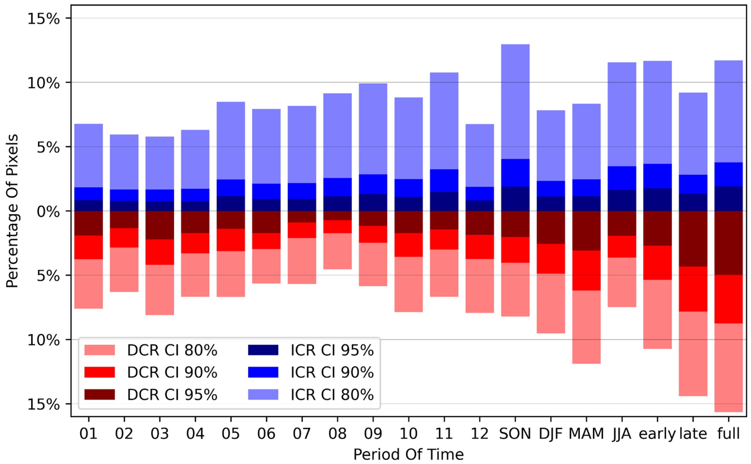
The pixel-based trend analysis was performed for all 119 tiles for the 19 seasons mentioned (a total of 2261 analyses). In order to determine which periods have a particularly large number of significant developments, the percentage of pixels that fall within the 95%, 90% and 80% confidence interval (CI) was determined both for increasing (ICR) and decreasing (DCR) developments of SCD. The result is shown in Figure 5.
As can be seen from Figure 5, there are no distinct seasons that are showing extreme developments, but in general, the monthly trends have less significant areas than the meteorological seasons. In turn, these have less significant developments than the snow-seasonal developments. This applies equally to all confidence levels. However, since the associated Theil–Sen slopes show very pronounced developments in some seasons, we will show the most interesting ones:
3.1.1. Pixel-Based SCD Trend for March (03)
In March, the SCD development is significant for 12% of the area in the 80% confidence level (3% in the 95% confidence level). Figure 6 shows the areas where significant developments are taking place and also indicates the magnitude of the developments.
The decrease in the SCD in the Baltic Sea region is particularly striking, and there are also significant decreases in the Siberian mountains, as well as in North America (from Lake Winnipeg to the Great Lakes). However, the large areas of increase in SCD in Central Asia are not significant.
3.1.2. Pixel-Based SCD Trend for April (04)
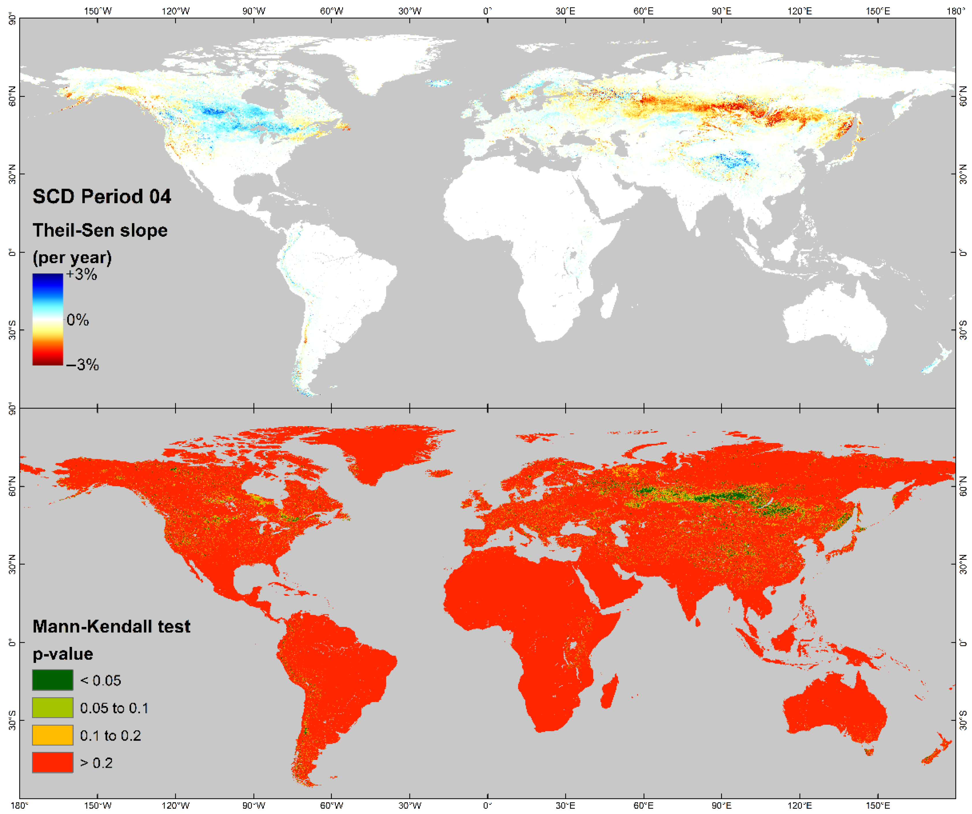
In April, the number of significant pixels is not extraordinarily high (11% at 80% confidence level, 3% at 95% confidence level). Figure 7 shows why this month is special.
In North America, particularly in southern Canada, large areas show an increase in SCD, although only few areas are significant. The situation is different in Eurasia. A mostly significant decrease in SCD can be observed over a broad strip stretching from the Baltic Sea over Lake Baikal to Japan.
3.1.3. Pixel-Based SCD Trend for November (11)
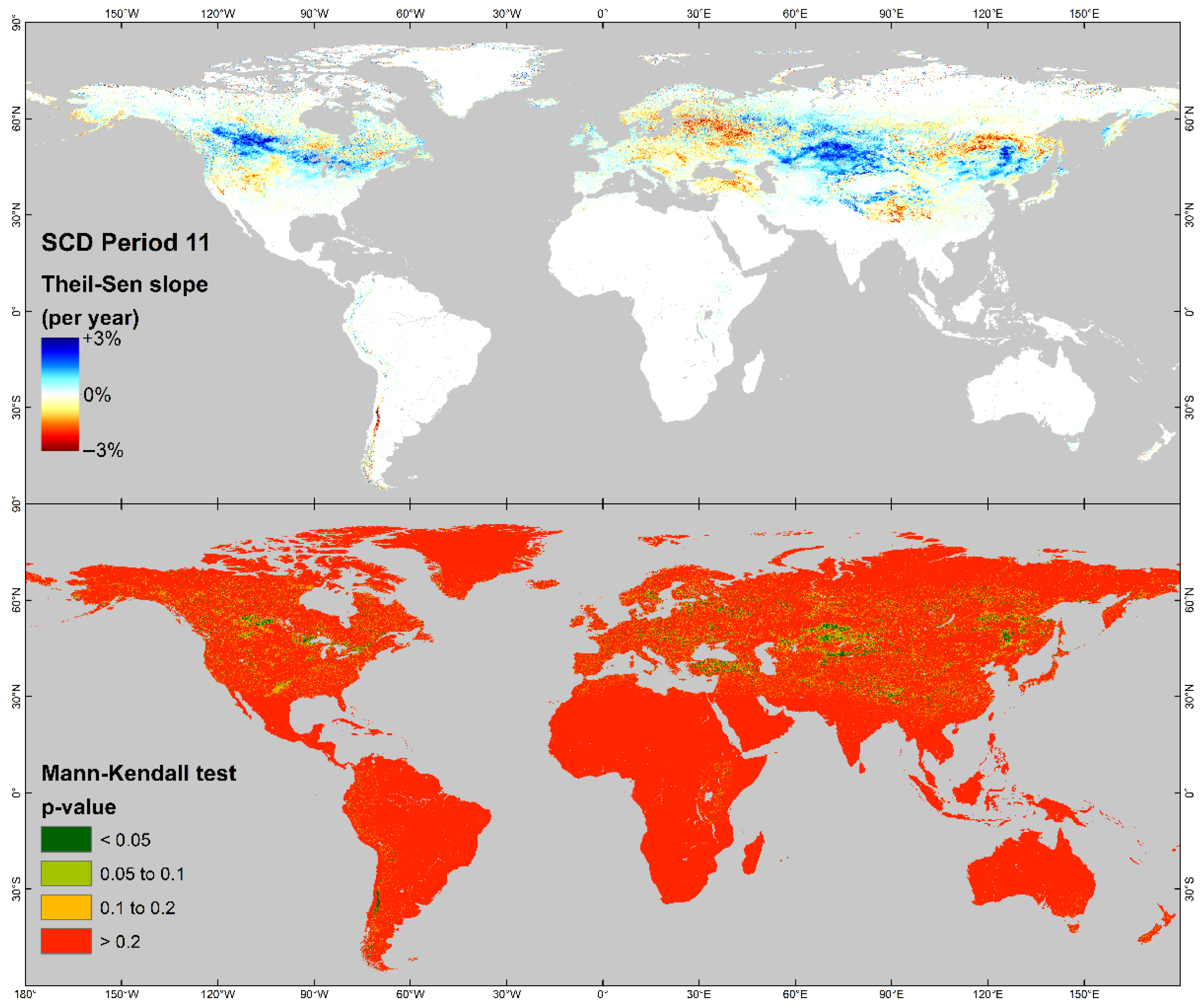
With 22% significant pixels (in the 80% confidence level), November shows the highest value in the monthly analysis (3% in the 95% confidence level). Figure 8 shows that this month is particularly marked by an increase in the SCD.
In November, a (mostly significant) increase in SCD is observed in much of Canada. A similarly strong increase can be seen in Central Asia and in China in the area of Manchuria.
3.1.4. Pixel-Based SCD Trend for Boreal Spring (MAM)
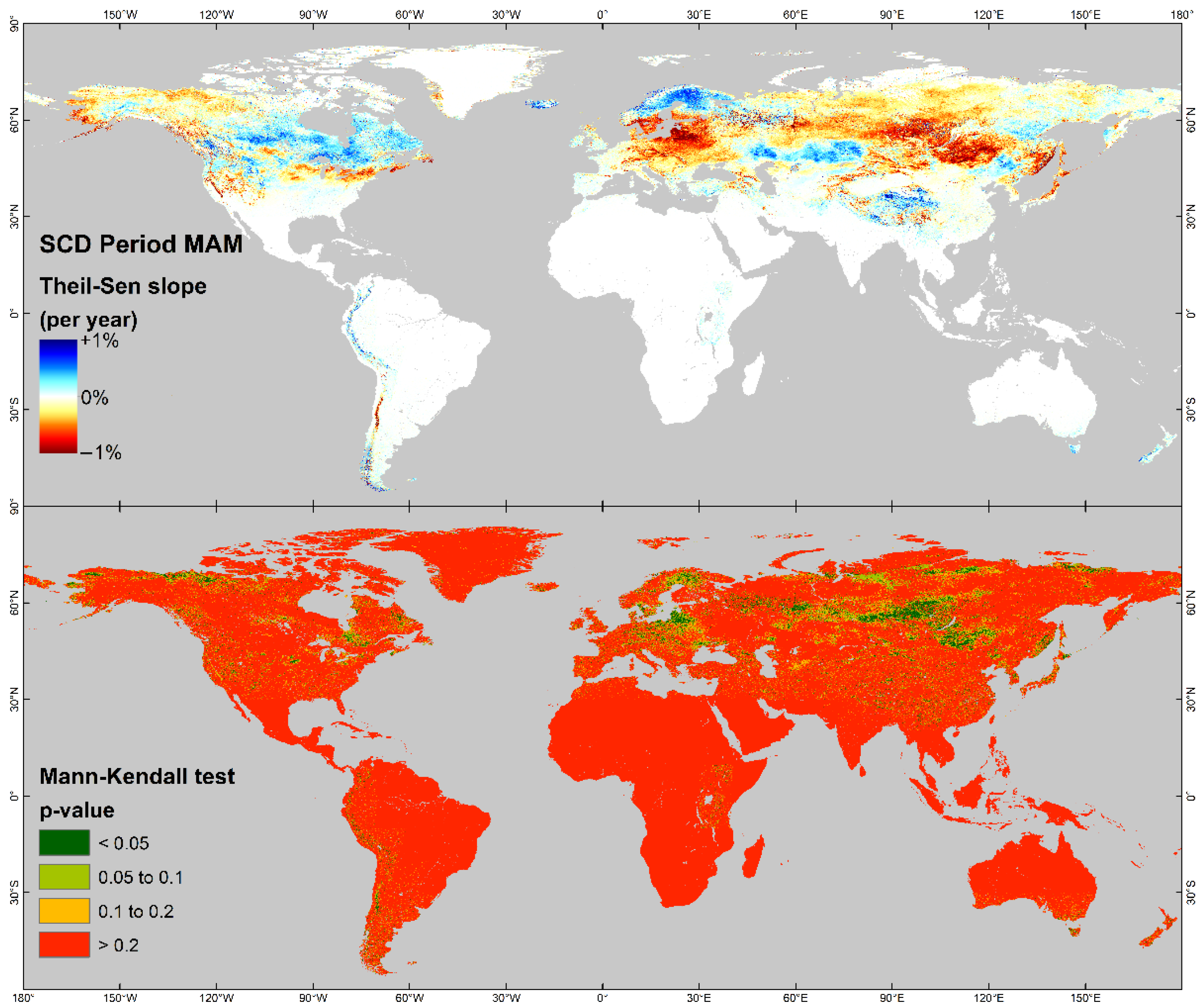
In the boreal spring (March–May), almost 18% of the pixels achieve significant developments of SCD (80% confidence level; 4.3% in the 95% confidence level). Figure 9 shows the development in this meteorological season.
While the prevailing increase in SCD in North America is not significant, the sometimes drastic SCD decreases in Eurasia are mostly significant. A significant increase can also be observed in northern Europe in the area of Sápmi.
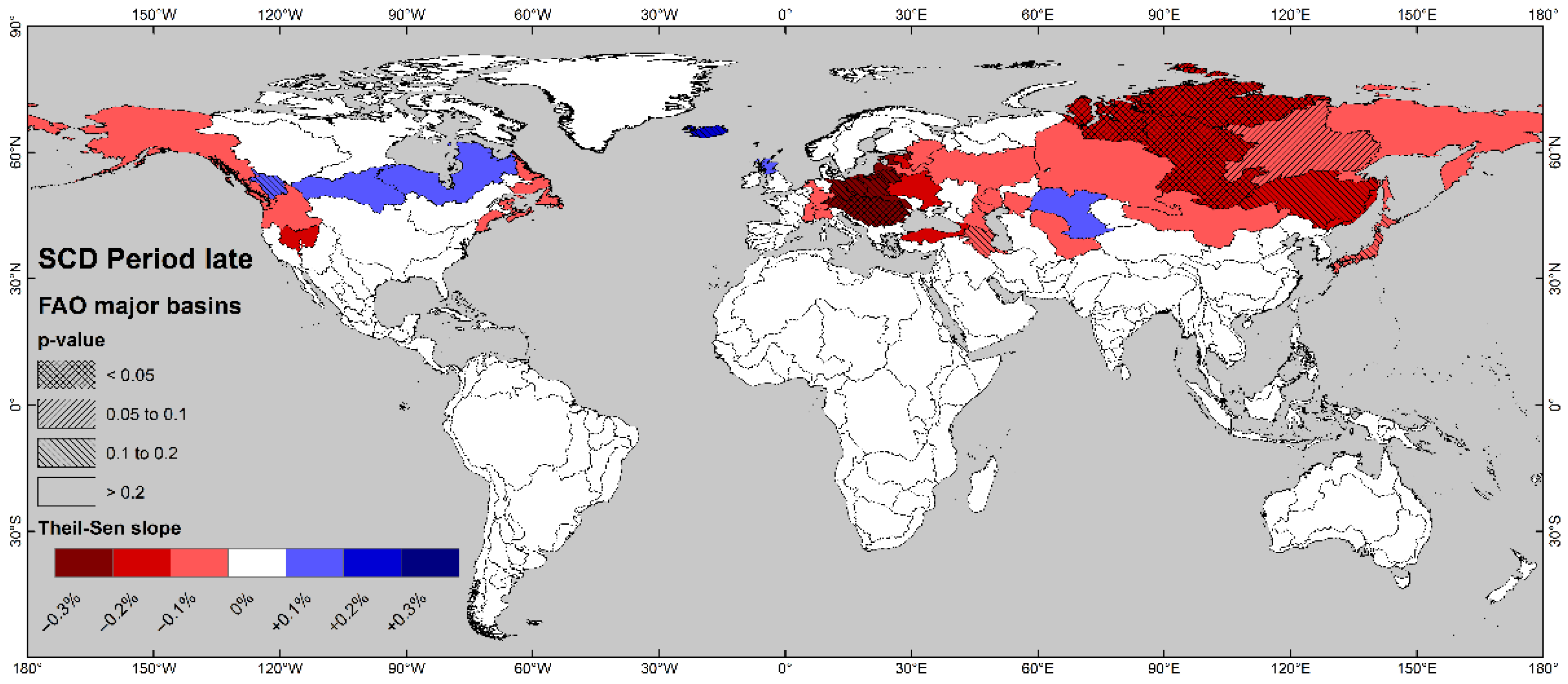
3.1.5. Pixel-Based SCD Trend for Late Snow Season
In the late snow season, 21% of the pixels show significant development at the 80% confidence level (6% at the 95% confidence level). Figure 10 shows the SCD developments.
This season, especially in the far north of Canada and Russia, there is a significant decrease in snow cover duration. The significant decrease in the Baltic Sea region, which was already determined for March, is also reflected here.
3.2. Basin-Based Analysis
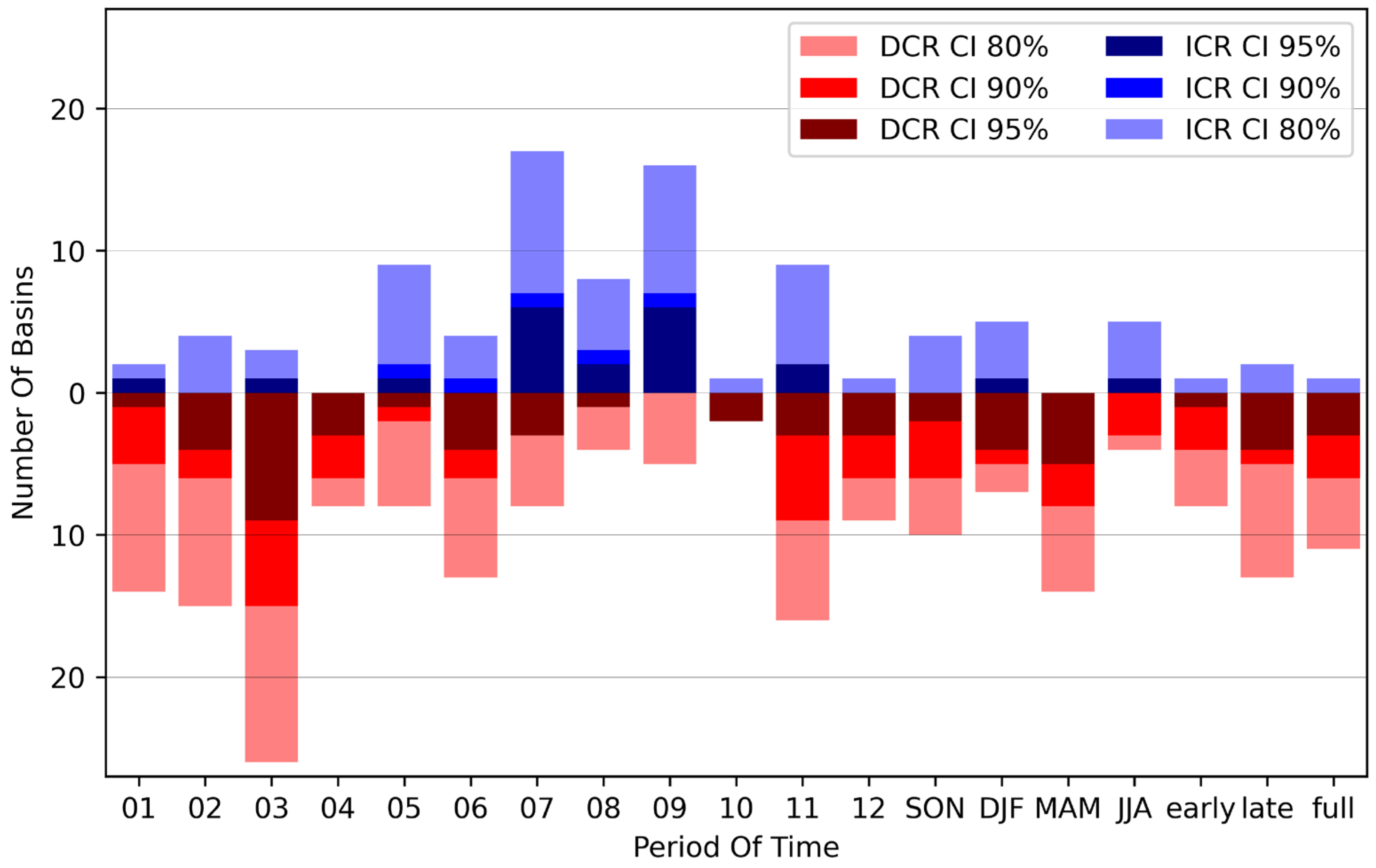
The SCD development averaged over all pixels of the 57 selected FAO main basin areas show in general similar results. However, in contrast to the pixel-based trend analysis, three periods of time are emerging in which a larger number of basins shows significant developments of SCD (Figure 11).
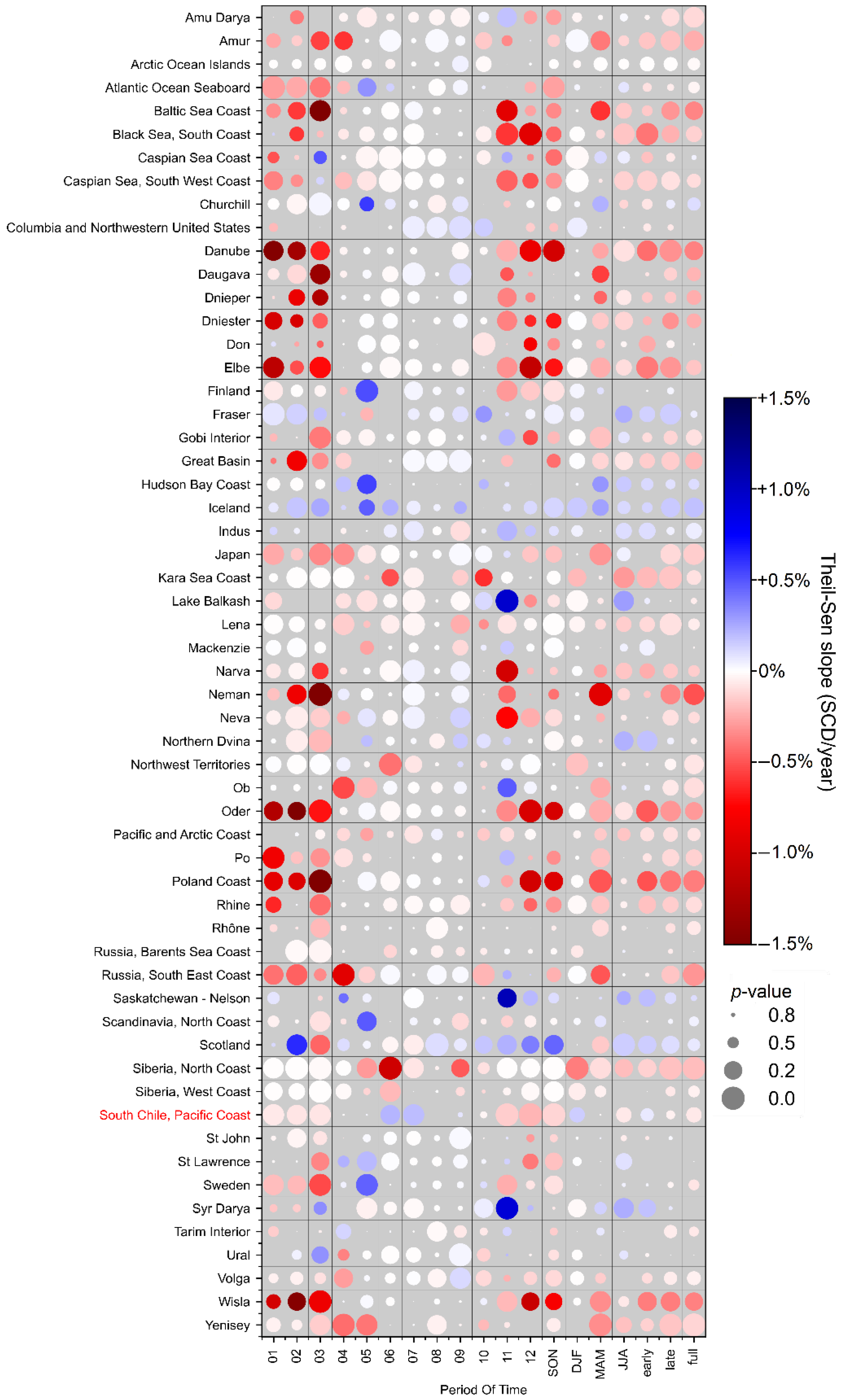
The two months of March and November, as well as the late snow season, stand out here and will be examined in more detail. Figure 12 summarizes the development of all 57 catchment areas for the 19 seasons.
3.2.1. Basin-Based SCD Trend for March
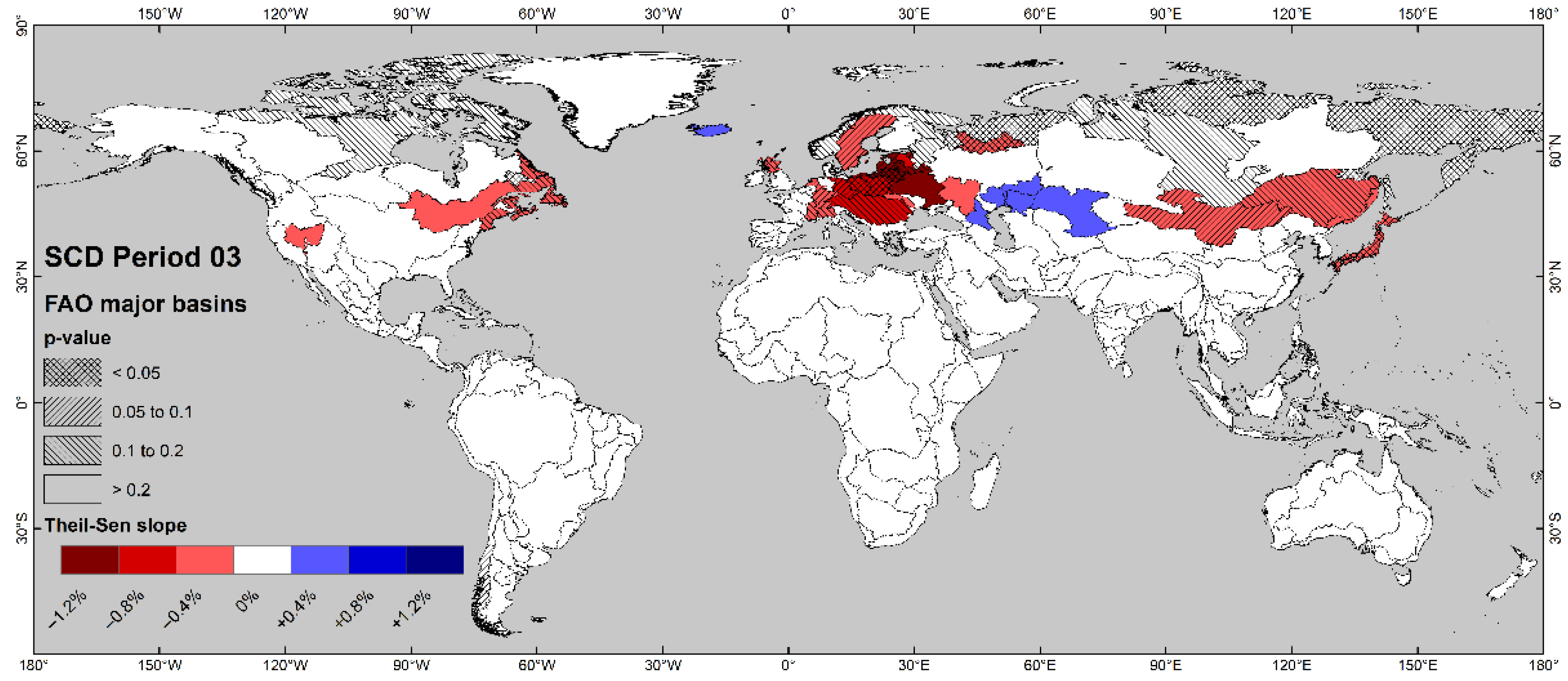
As already seen from the pixel-based analysis, the region surrounding the Baltic Sea in particular is a hotspot of the SCD decrease in March. This is also reflected in the analysis of the major basin areas for this month. A total of 18% of the examined basins show a significant development of the SCD in the 95% confidence level (almost 50% do so in the 80% confidence level). Figure 13 shows the magnitudes and significance for this month.
As mentioned, it is above all the catchment areas that drain into the Baltic Sea that the strongest trends are shown here. For Wisla, it is −0.26 days/year for this month; on the Poland coast, it is −0.47 days/year; and on the river Oder, it is −0.22 days/year. However, the catchment area of the Neman River, which flows through Belarus, Lithuania and the Russian enclave of Kaliningrad, has the strongest trend at −0.85 days/year. Positive trends can be seen in Iceland and some basins in Central Asia; however, their development is not significant.
3.2.2. Basin-Based SCD Trend for November
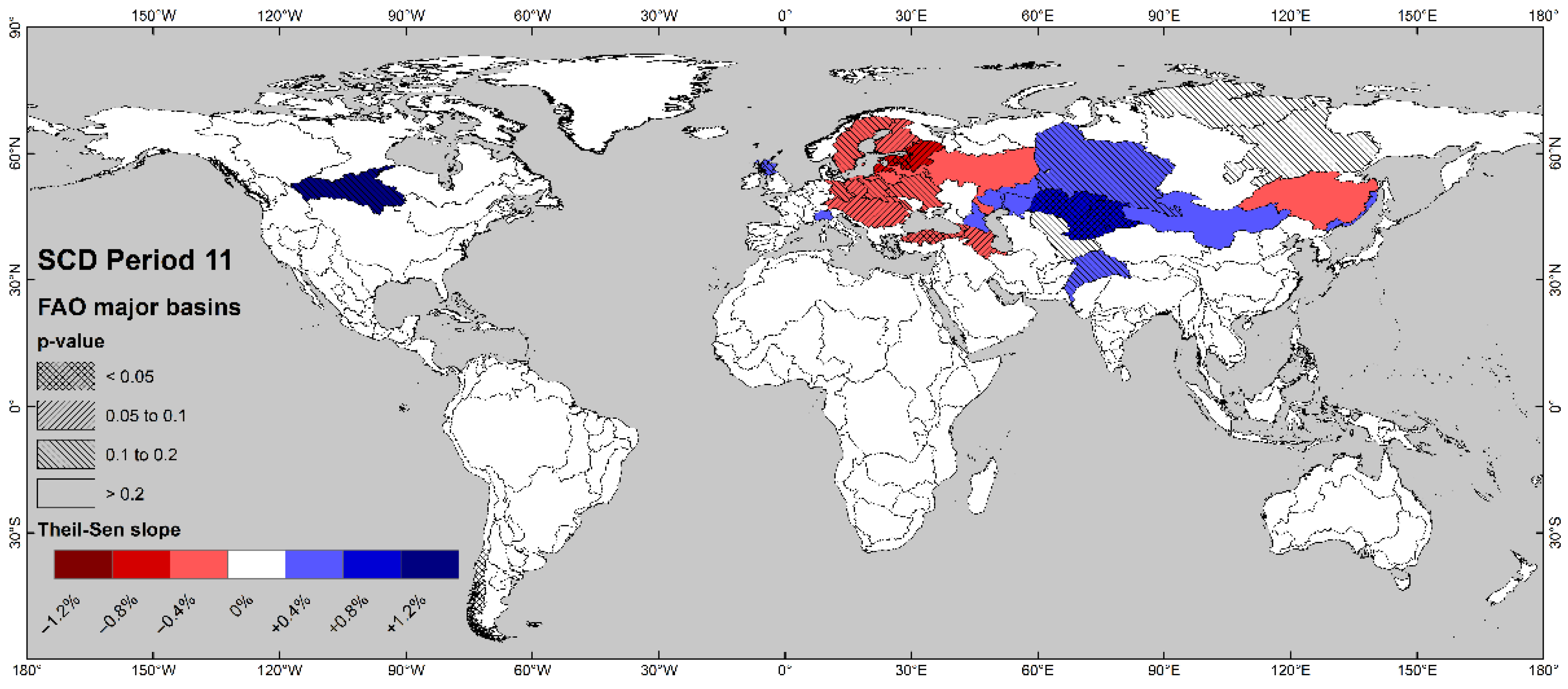
The month of November shows the second strongest trends with a significant development of 40% of all basin areas (in the 80% confidence level); however, only five catchment areas (9%) are significant in the 95% confidence level. Figure 14 shows the developments for the month of November.
The catchment areas of the Narva (the border river between Estonia and Russia) show significant negative developments this month with −0.3 days/year and the southern coast of the Black Sea with −0.18 days/year. However, the trends of two catchments in Central Asia are more striking: the Lake Balkash catchment at +0.29 days/year and the Syr Darya catchment at +0.27 days/year. The maximum significant SCD increase (within the 80% confidence level) shows the catchment area of the Nelson River in Canada/Unite States with +0.31 days/year.
3.2.3. Basin-Based SCD Trend for Late Snow Season
In terms of snow seasons, the late season SCD shows the most significant developments with 26% of all basins in the 80% confidence level (7% on the 95% confidence level). Figure 15 shows the developments for the late season SCD.
When considering the catchment areas, the trends for March are also reflected in the late season SCD. This applies to the catchment areas of the Baltic Sea. The largest decrease in the 95% confidence level shows the Danube with −0.95 days/year, followed by the Siberian North Coast with −0.54 days/year and the Kara Sea Coast with −0.52 days/year. Additionally, the fourth largest basin of this study—the river Yenisey—shows a significant decrease in SCD with −0.50 days/year. Positive trends occur again in basins in southern Canada, but they are not significant.
4. Discussion
The first research question was to answer whether the now 23-year data set of complete GSP data is sufficient to identify reliable trends. We are aware that the 30-year Climate Normal (CN) [53] determined by the WMO (the youngest completed is 1991–2020) were chosen in order to be able to make secured statements, and that our data set is of course smaller. Nevertheless, we want to put our results in this context. The global trend analysis of mountain areas of the SCD examined by [22] covered 38 years (1982–2020). A mean trend of −0.4 days/year was observed for this period, which agrees well with our pixel-based trend for the whole SCD of −0.44 days/year. We also succeeded in confirming the snow cover changes in Europe predicted by [54] based on regional climate models. As in their simulations, the Baltic Sea region turns out to be a hotspot for changing SCD, they see an SCD decrease of −0.55 days/year over 60 years for the CN 2071–2100 compared to CN 1961–1990. We found the largest significant decreases for the basin areas in the boreal spring and March. The Poland coast showed a similar decrease for this period of −0.47 days/year, while the Neman river was almost twice as much at −0.85 days/year. The SCD increase in northern Fennoscandia in the boreal spring shown in Figure 9 confirms previous studies [26]. For the continental areas in Canada, the SCD increase found by [27] in the boreal spring (Figure 9) could be confirmed. However, e.g., the Nelson River showed a significant SCD increase of +0.31 days/year even in November, where [27] found a general decrease. In the month of November, the continental basins of Syr Darya and Lake Balkash in Asia also stood out with significant SCD increases (Figure 14). For Syr Darya, we found +0.27 days/year, which corresponds to the findings of the 28-year time series from [45]. The Lake Balkash catchment SCD increase of +0.29 days/year coincides with a climate change induced precipitation increase in this region of +0.654 mm/year [55]. The general SCD increase in Northeast China (NEC) in the Manchurian region also has climatological causes (see Figure 8, Figure 9 and Figure 10). This is attributed by [56] (who studied the period 1985–2010) to a weakening of the East Asian Winter Monsoon (EAWM), which allows colder air to penetrate from the north. Along with increased water vapor content, this leads to increased snowfall in NEC. The comparisons with previous, mostly regional studies over longer periods of time show that our results of the 23 examined years confirmed previous findings but also new trends could be identified; 23 years are therefore sufficiently well suited to depicting trends.
The next point to discuss is the accuracy, on the one hand of the MODIS data itself, on the other hand of the gap-filled product. The absolute accuracy of this product is given by [57] as >93% depending on the land cover. The accuracy of MODIS on Aqua is slightly lower due to the defective band 6. In order to reliably determine trends, a correction for the gaps due to cloud cover is essential, since in Europe, for example, these cover 46.86% of the pixels for Terra and 48.47% for Aqua [43]. In the first step, the daily combination of Terra and Aqua, the accuracy remains at 92% [58,59]. The 3-day interpolation leads to hardly any deterioration in accuracy, and that of the topographical interpolation is given by [60] with 95%. Filling the remaining gaps with the pixel values of preceding days has a greater influence on the accuracy. The accuracy drops with increasing time steps, a cloud-persistence count (CPC) layer is included in our and the CGF product [61]. The filling of cloud gaps occurs mainly in the first few days with an exponential decrease. In the example from [61], 90% of the gaps were filled after just 5 days. After 10 days, there are usually no more gaps. A study by [3] in Chile was therefore satisfied with a temporal filling of up to 3 days and obtained almost cloud-free snow coverage. During the polar night, the gaps are of course larger, but due to the usually continuous snow cover during this time, there is no loss of accuracy either. The gap-free SCD is validated either indirectly with weighted individual accuracies of the different steps [58,62], or directly with measuring stations on the ground. The latter are unfortunately very unequally distributed or are missing entirely. In comparison with station data, [59] achieved an accuracy of 92.79–93.34% for the gap-free SCD data set in China; for the described GSP product, an accuracy of 86.66% was achieved for Europe (station data mainly exist in the Netherlands and Norway) [43]. For Chile the overall accuracy was between 81 and 92% [63]. For our global approach, np analysis of the accuracy was carried out so far, and due to the examined areas, only indirect validation is possible. An estimation of the accuracy based on the CPC is still in progress.
The next point is to discuss whether the chosen approach, which combines the MK test and Theil–Sen slope, is suitable. The combination of these has often been used for snow surface dynamics [17,64,65], but it also means that some developments remain undetected. Larger interannual SCD variations and fluctuations lead to a lower significance and are therefore not noticeable in such a large data set. On a regional scale, however, these strong fluctuations can already have catastrophic hydrological effects such as floods or droughts, as has been shown in [26]. The strength, or even the weakness, of the Theil–Sen slope calculation lies in the fact that such extremes are filtered out—even if these are not real outliers, but only reflect the natural variability. Alternatively, it would be advisable to rather use the coefficient of variance (CV; the standard deviation divided by the mean) [66]. This would also allow to better assess the significance of SCD changes, since, for example, one day less SCD per year has a smaller impact in the Arctic than in the central European low mountain ranges. There is also the question of whether the choice of catchment areas as aggregation makes sense. From a hydrological point of view, this has definitely proven to be the case [28,29], but the set threshold values meant that only one basin in the southern hemisphere was examined. For the southern hemisphere, an investigation of mountainous areas as in [22] would therefore make more sense, since there is no extensive snow cover in the lowlands—but most of the seasonal snow cover occurs in the lowlands of the northern hemisphere [67]. This leads to the desired follow-up investigations, which are to be carried out with the data set (and the additional years).
In the future, evaluations should therefore be carried out according to altitude as well as meridional and zonal classification. Of course, this is then no longer globally feasible, but is applied to selected catchment areas that were shown in this study. The relatively snow-poor areas of the southern hemisphere should be considered by examining the global mountain ranges in a further study in order to be able to compare the results of the GSP processor directly with the work of [22]. Together with information on flora (NDVI and land cover classes), the influence of snow development on vegetation development is to be examined with regard to the important topic of greening of the Arctic [68].
5. Conclusions
In summary, it was found that the 23 years that are now available are already sufficient to determine significant trends for a considerable part of the observed areas. This was possible for the snow cover duration of the entire hydrological year in the 80% confidence interval for almost 25% of the observed area (pixel-based). For the sometimes very large (an aggregated) major basin areas of the FAO data set, it was shown that these are very well suited to interpreting the snow cover development averaged over the entire catchment area. Nevertheless, of course this study cannot replace detailed hydrological modeling (with additional area properties and meteorological conditions), and a closer look should certainly at least consider the relief dependency. However, we are showing an easy-to-implement possibility to achieve a global overview of basin-dependent SCD developments—and then to take a closer look at interesting basins. For both the pixel-based and basin-based analysis, we found a global general decrease in SCD. In some areas, there was also a shift in the snow cover season (earlier onset or delayed melt) with roughly the same overall duration.
Author Contributions
Conceptualization, S.R. and A.J.D.; methodology, S.R.; software, S.R.; formal analysis, A.J.D.; data curation, S.R.; writing—original draft preparation, S.R.; writing—review and editing, A.J.D.; visualization, S.R.; supervision, A.J.D.; project administration, A.J.D.; funding acquisition, A.J.D. All authors have read and agreed to the published version of the manuscript.
Funding
This research was funded by the internal DLR “Polar Monitor” project.
Institutional Review Board Statement
Not applicable.
Informed Consent Statement
Not applicable.
Data Availability Statement
Daily MODIS snow information is provided by the National Snow and Ice Data Center (NSIDC) is freely available from Terra (https://nsidc.org/data/mod10a1/versions/61; accessed on 15 September 2022) and Aqua (https://nsidc.org/data/myd10a1/versions/61; accessed on 15 September 2022). The results of the latest version of the gap-free product GSPare available on the DLR’s GeoService (https://geoservice.dlr.de; accessed on 20 November 2022). For visualization, the daily product can be displayed on https://geoservice.dlr.de/web/maps/eoc:gsp:daily (accessed on 20 November 2022), the yearly accumulated snow cover durations (SCDs) on https://geoservice.dlr.de/web/maps/eoc:gsp:yearly (accessed on 20 November 2022).
Acknowledgments
We sincerely thank the scientific editor for his valuable comments and suggestions for improvement. Many thanks also go to the three anonymous reviewers who significantly improved the manuscript with their detailed comments.
Conflicts of Interest
The authors declare no conflict of interest.
Appendix A
The Mann–Kendall (MK) test [49,50] is used to determine whether there is a monotonic trend in a time series, and the Theil–Sen slope [51] is used to determine the magnitude of the trend. In the MK test, the null hypothesis (H0) indicates no trend, while the alternative hypothesis indicates the presence of a trend. In the following, and stand for two consecutive years (where is later than ), and stand for the SCD of the corresponding years. First, the strength of the sequence for the time series is described by the MK statistic S is derived from Equations (A1) to (A2) [48]:
After that, the variance of depending on the number of years is calculated using Equation (A3):
Finally, the statistic is calculated from and , which states whether there is a positive or negative trend (Equation (A4)):
The trend is significant when , where is the significance level corresponding to the -value and can be set to e.g., 0.05. Finally, the magnitude of the trend () is calculated by the Theil–Sen slope (Equation (A5)):
Appendix B
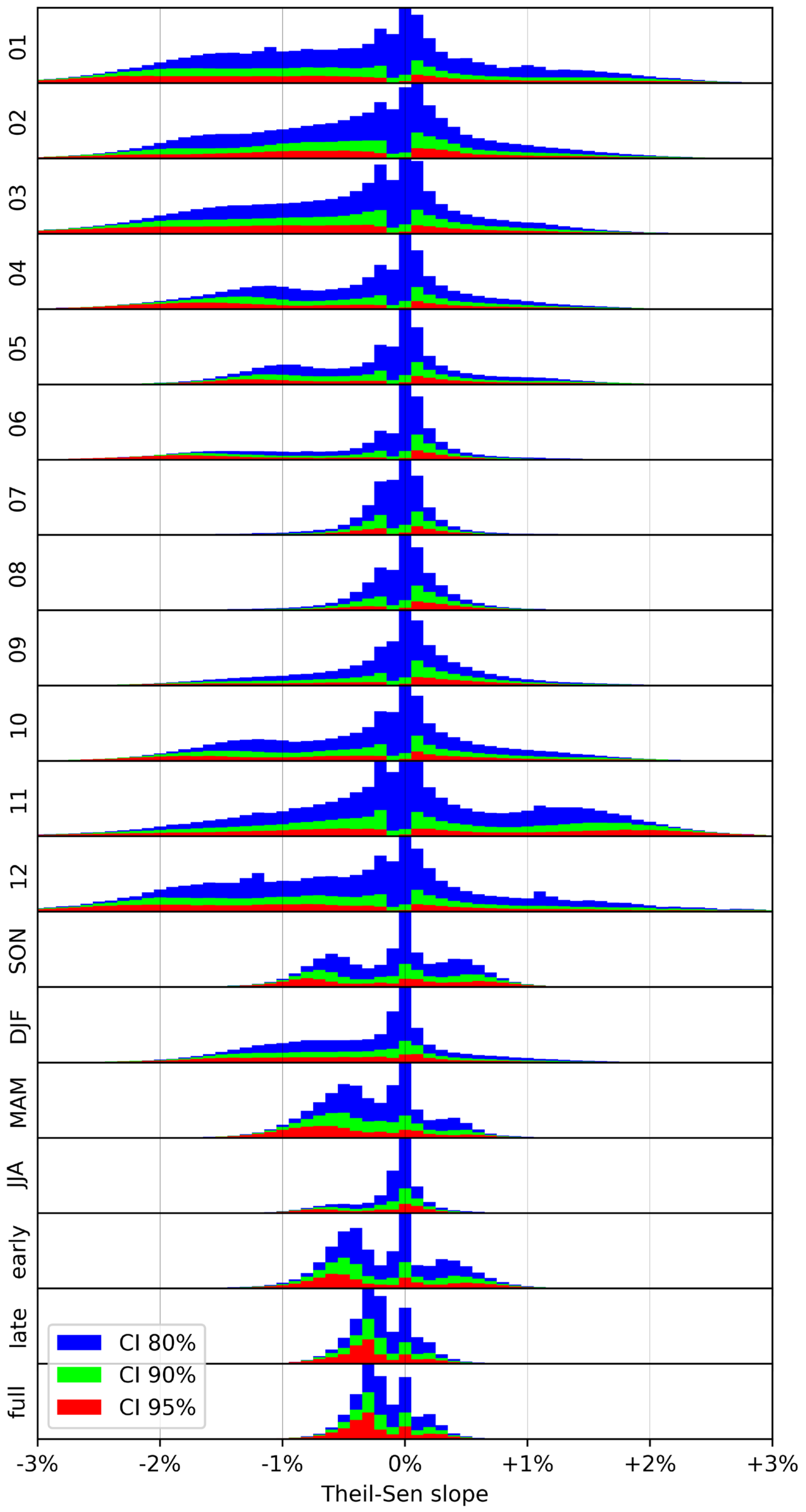
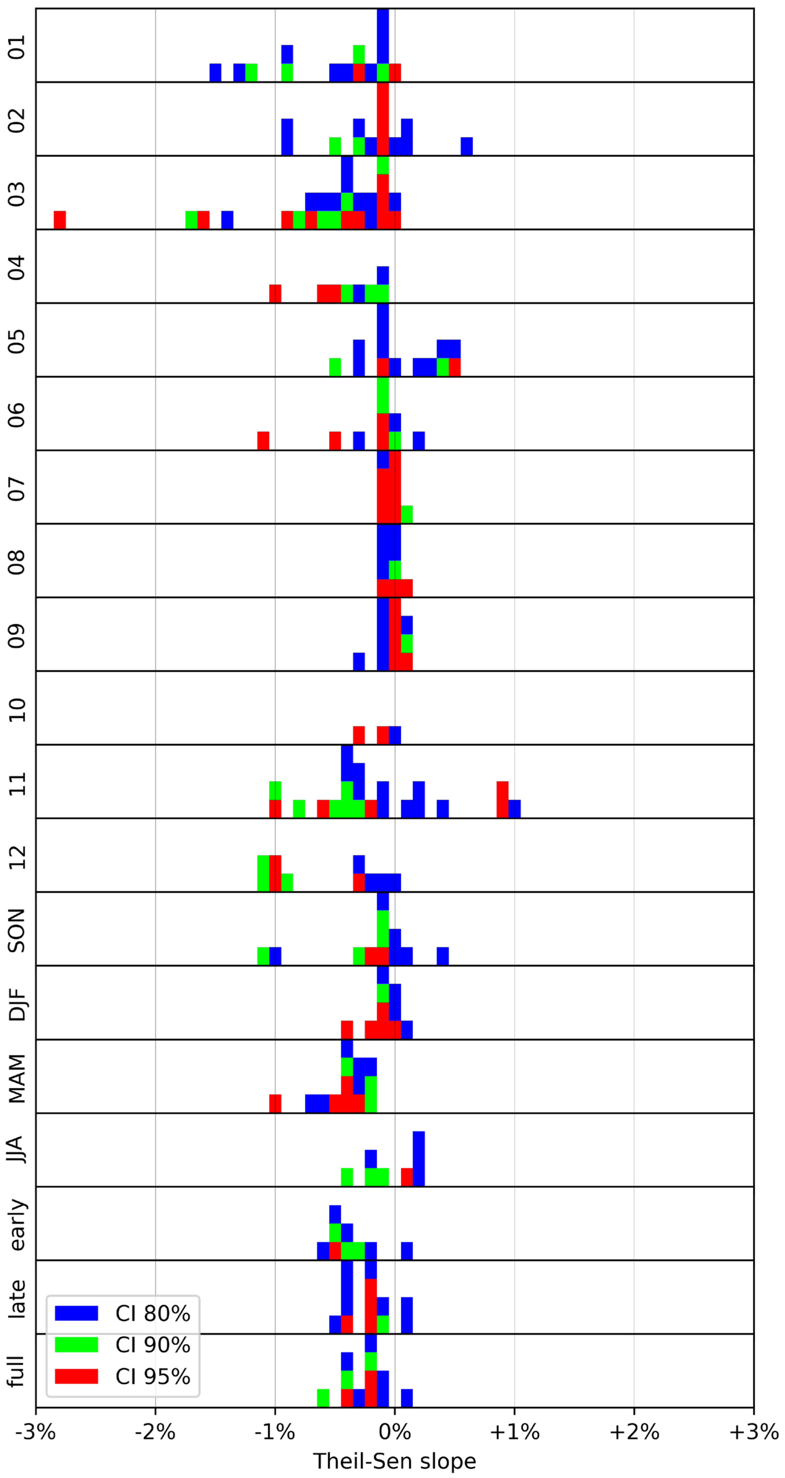
Since, for the sake of clarity, only the most relevant time periods are presented in the manuscript, the histograms for the pixel- and basin-based analysis are shown below. Figure A1 shows the histograms of the pixel-based analysis, Figure A2 shows the histograms of the basin-based analysis. In addition, Table A1 and Table A2 show the mean slope values for the time periods and confidence intervals.
Figure A1.
Histograms of derived Theil–Sen slopes of the pixel-based trend analysis of SCD for the 19 observed periods. The color coding represents the confidence intervals, and a normalization with the largest value was carried out.
Figure A1.
Histograms of derived Theil–Sen slopes of the pixel-based trend analysis of SCD for the 19 observed periods. The color coding represents the confidence intervals, and a normalization with the largest value was carried out.

Figure A2.
Histograms of derived Theil–Sen slopes of the basin-based trend analysis of SCD for the 19 observed periods. The color coding represents the confidence intervals, and a normalization with the largest value was carried out.
Figure A2.
Histograms of derived Theil–Sen slopes of the basin-based trend analysis of SCD for the 19 observed periods. The color coding represents the confidence intervals, and a normalization with the largest value was carried out.


Table A1.
Arithmetic mean of the slopes (scaled to days per year) of the pixel-based trend analysis for the three confidence intervals. Note that the pixels are a percentage of the total (not the total number N).
Table A1.
Arithmetic mean of the slopes (scaled to days per year) of the pixel-based trend analysis for the three confidence intervals. Note that the pixels are a percentage of the total (not the total number N).
| Period | CI 80% [Days/Year] (%) | CI 90% [Days/Year] (%) | CI 95% [Days/Year] (%) |
|---|---|---|---|
| 01 | −0.12 (13%) | −0.18 (6%) | −0.23 (3%) |
| 02 | −0.09 (11%) | −0.12 (5%) | −0.14 (2%) |
| 03 | −0.16 (12%) | −0.22 (6%) | −0.27 (3%) |
| 04 | −0.10 (11%) | −0.17 (5%) | −0.22 (2%) |
| 05 | −0.05 (13%) | −0.07 (6%) | −0.07 (3%) |
| 06 | −0.09 (11%) | −0.16 (5%) | −0.24 (3%) |
| 07 | −0.01 (12%) | −0.01 (4%) | −0.01 (2%) |
| 08 | 0.00 (11%) | 0.00 (4%) | −0.00 (2%) |
| 09 | −0.02 (13%) | −0.04 (5%) | −0.05 (2%) |
| 10 | −0.07 (14%) | −0.11 (6%) | −0.14 (3%) |
| 11 | 0.03 (14%) | 0.04 (6%) | 0.03 (3%) |
| 12 | −0.12 (13%) | −0.17 (6%) | −0.22 (3%) |
| SON | −0.04 (17%) | −0.07 (8%) | −0.11 (4%) |
| DJF | −0.29 (15%) | −0.40 (7%) | −0.48 (4%) |
| MAM | −0.20 (18%) | −0.28 (9%) | −0.35 (4%) |
| JJA | −0.07 (16%) | −0.12 (7%) | −0.17 (4%) |
| early | −0.14 (19%) | −0.18 (9%) | −0.22 (4%) |
| late | −0.33 (21%) | −0.43 (11%) | −0.52 (6%) |
| full | −0.44 (24%) | −0.57 (13%) | −0.69 (7%) |
Table A2.
Arithmetic mean of the slopes (scaled to days per year) of the basin-based trend analysis for the three confidence intervals. N shows the total number of basin areas.
Table A2.
Arithmetic mean of the slopes (scaled to days per year) of the basin-based trend analysis for the three confidence intervals. N shows the total number of basin areas.
| Period | CI 80% [Days/Year] (N) | CI 90% [Days/Year] (N) | CI 95% [Days/Year] (N) |
|---|---|---|---|
| 01 | −0.15 (15) | −0.13 (6) | −0.03 (2) |
| 02 | −0.03 (19) | −0.04 (6) | −0.01 (4) |
| 03 | −0.16 (28) | −0.20 (16) | −0.20 (10) |
| 04 | −0.10 (8) | −0.12 (6) | −0.19 (3) |
| 05 | 0.03 (15) | 0.04 (4) | 0.08 (2) |
| 06 | −0.03 (16) | −0.06 (7) | −0.11 (4) |
| 07 | 0.00 (18) | 0.01 (10) | 0.00 (9) |
| 08 | 0.00 (9) | 0.01 (4) | 0.01 (3) |
| 09 | 0.00 (14) | 0.02 (7) | 0.01 (6) |
| 10 | −0.03 (3) | −0.04 (2) | −0.04 (2) |
| 11 | −0.03 (23) | −0.08 (11) | 0.01 (5) |
| 12 | −0.17 (10) | −0.26 (6) | −0.22 (3) |
| SON | −0.13 (14) | −0.23 (6) | −0.06 (2) |
| DJF | −0.03 (11) | −0.09 (6) | −0.10 (5) |
| MAM | −0.33 (14) | −0.33 (8) | −0.42 (5) |
| JJA | 0.02 (8) | −0.10 (4) | 0.13 (1) |
| early | −0.42 (9) | −0.51 (4) | −0.55 (1) |
| late | −0.42 (15) | −0.42 (5) | −0.48 (4) |
| full | −0.72 (12) | −1.02 (6) | −0.77 (3) |
References
- Hall, D.K.; Riggs, G.A.; Salomonson, V.V. Development of methods for mapping global snow cover using moderate resolution imaging spectroradiometer data. Remote Sens. Environ. 1995, 54, 127–140. [Google Scholar] [CrossRef]
- Pepe, M.; Brivio, P.A.; Rampini, A.; Nodari, F.R.; Boschetti, M. Snow cover monitoring in alpine regions using ENVISAT optical data. Int. J. Remote Sens. 2005, 26, 4661–4667. [Google Scholar] [CrossRef]
- Goodrich, L.E. The influence of snow cover on the ground thermal regime. Can. Geotech. J. 1982, 19, 421–432. [Google Scholar] [CrossRef] [Green Version]
- GCOS, WMO. Systematic Observation Requirements for Satellite-Based Data Products for Climate—2011 Update; GCOS, WMO: Geneva, Switzerland, 2011. [Google Scholar]
- Mankin, J.S.; Viviroli, D.; Singh, D.; Hoekstra, A.Y.; Diffenbaugh, N.S. The potential for snow to supply human water demand in the present and future. Environ. Res. Lett. 2015, 10, 114016. [Google Scholar] [CrossRef]
- Winkler, D.E.; Butz, R.J.; Germino, M.J.; Reinhardt, K.; Kueppers, L.M. Snowmelt timing regulates community composition, phenology, and physiological performance of alpine plants. Front. Plant Sci. 2018, 9, 1140. [Google Scholar] [CrossRef] [Green Version]
- Elder, K.; Dozier, J.; Michaelsen, J. Snow accumulation and distribution in an alpine watershed. Water Resour. Res. 1991, 27, 1541–1552. [Google Scholar] [CrossRef] [Green Version]
- Dietz, A.J.; Kuenzer, C.; Gessner, U.; Dech, S. Remote sensing of snow—A review of available methods. Int. J. Remote Sens. 2012, 33, 4094–4134. [Google Scholar] [CrossRef]
- Painter, T.H.; Berisford, D.F.; Boardman, J.W.; Bormann, K.J.; Deems, J.S.; Gehrke, F.; Hedrick, A.; Joyce, M.; Laidlaw, R.; Marks, D.; et al. The airborne snow observatory: Fusion of scanning lidar, imaging spectrometer, and physically-based modeling for mapping snow water equivalent and snow albedo. Remote Sens. Environ. 2016, 184, 139–152. [Google Scholar] [CrossRef] [Green Version]
- Chang, A.T.C.; Foster, J.L.; Hall, D.K.; Robinson, D.A.; Peiji, L.; Meisheng, C. The use of microwave radiometer data for characterizing snow storage in Western China. Ann. Glaciol. 1992, 16, 215–219. [Google Scholar] [CrossRef] [Green Version]
- Kelly, R.E.; Chang, A.T.; Tsang, L.; Foster, J.L. A prototype AMSR-e global snow area and snow depth algorithm. IEEE Trans. Geosci. Remote Sens. 2003, 41, 230–242. [Google Scholar] [CrossRef]
- Tsai, Y.L.S.; Dietz, A.; Oppelt, N.; Kuenzer, C. Wet and dry snow detection using Sentinel-1 SAR data for mountainous areas with a machine learning technique. Remote Sens. 2019, 11, 895. [Google Scholar] [CrossRef] [Green Version]
- Koehler, J.; Bauer, A.; Dietz, A.J.; Kuenzer, C. Towards forecasting future snow cover dynamics in the European Alps—The potential of long optical remote-sensing time series. Remote Sens. 2022, 14, 4461. [Google Scholar] [CrossRef]
- Hall, D.K.; Riggs, G.A.; Salomonson, V.V.; DiGirolamo, N.E.; Bayr, K.J. MODIS snow-cover products. Remote Sens. Environ. 2002, 83, 181–194. [Google Scholar] [CrossRef] [Green Version]
- Ackroyd, C.; Skiles, S.M.; Rittger, K.; Meyer, J. Trends in snow cover duration across river basins in high mountain asia from daily Gap-Filled MODIS fractional snow covered area. Front. Earth Sci. 2021, 9, 713145. [Google Scholar] [CrossRef]
- Malmros, J.K.; Mernild, S.H.; Wilson, R.; Tagesson, T.; Fensholt, R. Snow cover and snow Albedo changes in the central andes of Chile and Argentina from Daily MODIS Observations (2000–2016). Remote Sens. Environ. 2018, 209, 240–252. [Google Scholar] [CrossRef] [Green Version]
- Saavedra, F.A.; Kampf, S.K.; Fassnacht, S.R.; Sibold, J.S. Changes in andes snow cover from MODIS data, 2000–2016. Cryosphere 2018, 12, 1027–1046. [Google Scholar] [CrossRef] [Green Version]
- Xiao, L.; Che, T.; Chen, L.; Xie, H.; Dai, L. Quantifying snow albedo radiative forcing and its feedback during 2003–2016. Remote Sens. 2017, 9, 883. [Google Scholar] [CrossRef] [Green Version]
- Zhou, H.; Aizen, E.; Aizen, V. Deriving long term snow cover extent dataset from AVHRR and MODIS data: Central Asia case study. Remote Sens. Environ. 2013, 136, 146–162. [Google Scholar] [CrossRef]
- Premier, V.; Marin, C.; Steger, S.; Notarnicola, C.; Bruzzone, L. A novel approach based on a hierarchical multiresolution analysis of optical time series to reconstruct the daily high-resolution snow cover area. IEEE J. Sel. Top. Appl. Earth Obs. Remote Sens. 2021, 14, 9223–9240. [Google Scholar] [CrossRef]
- Revuelto, J.; Alonso-González, E.; Gascoin, S.; Rodríguez-López, G.; López-Moreno, J.I. Spatial downscaling of MODIS snow cover observations using Sentinel-2 snow products. Remote Sens. 2021, 13, 4513. [Google Scholar] [CrossRef]
- Notarnicola, C. Overall negative trends for snow cover extent and duration in global mountain regions over 1982–2020. Sci Rep 2022, 12, 13731. [Google Scholar] [CrossRef] [PubMed]
- Hall, D.K.; Riggs, G.A.; Foster, J.L.; Kumar, S.V. Development and evaluation of a cloud-gap-filled MODIS daily snow-cover product. Remote Sens. Environ. 2010, 114, 496–503. [Google Scholar] [CrossRef] [Green Version]
- Dietz, A.J.; Kuenzer, C.; Dech, S. Global SnowPack: A new set of snow cover parameters for studying status and dynamics of the planetary snow cover extent. Remote Sens. Lett. 2015, 6, 844–853. [Google Scholar] [CrossRef]
- Dunn, R.J.H.; Aldred, F.; Gobron, N.; Miller, J.B.; Willett, K.M.; Ades, M.; Adler, R.; Allan, R.P.; Allan, R. Global climate. Bull. Am. Meteorol. Soc. 2021, 102, S11–S142. [Google Scholar] [CrossRef]
- Rößler, S.; Witt, M.S.; Ikonen, J.; Brown, I.A.; Dietz, A.J. Remote sensing of snow cover variability and its influence on the Runoff of Sápmi’s Rivers. Geosciences 2021, 11, 130. [Google Scholar] [CrossRef]
- Brown, R.D.; Smith, C.; Derksen, C.; Mudryk, L. Canadian in situ snow cover trends for 1955–2017 including an assessment of the impact of automation. Atmos. Ocean 2021, 59, 77–92. [Google Scholar] [CrossRef]
- Atif, I.; Iqbal, J.; Mahboob, M. Investigating snow cover and hydrometeorological trends in contrasting hydrological regimes of the Upper Indus Basin. Atmosphere 2018, 9, 162. [Google Scholar] [CrossRef] [Green Version]
- Blahušiaková, A.; Matoušková, M.; Jenicek, M.; Ledvinka, O.; Kliment, Z.; Podolinská, J.; Snopková, Z. Snow and climate trends and their impact on seasonal runoff and hydrological drought types in selected mountain catchments in Central Europe. Hydrol. Sci. J. 2020, 65, 2083–2096. [Google Scholar] [CrossRef]
- Desinayak, N.; Prasad, A.K.; El-Askary, H.; Kafatos, M.; Asrar, G.R. Snow cover variability and trend over the Hindu Kush Himalayan Region using MODIS and SRTM data. Ann. Geophys. 2022, 40, 67–82. [Google Scholar] [CrossRef]
- Niu, G.-Y.; Yang, Z.-L. An observation-based formulation of snow cover fraction and its evaluation over large north american river basins. J. Geophys. Res. 2007, 112, D21101. [Google Scholar] [CrossRef]
- Hoogeveen, J.; Faurès, J.-M.; Peiser, L.; Burke, J.; van de Giesen, N. GlobWat—A Global Water Balance Model to Assess Water Use in Irrigated Agriculture. Hydrol. Earth Syst. Sci. 2015, 19, 3829–3844. [Google Scholar] [CrossRef] [Green Version]
- Wang, L.; Lv, A. Identification and diagnosis of transboundary river basin water management in china and neighboring countries. Sustainability 2022, 14, 12360. [Google Scholar] [CrossRef]
- Hall, D.K.; Riggs, G.A. Normalized-Difference Snow Index (NDSI). In Encyclopedia of Snow, Ice and Glaciers; Singh, V.P., Singh, P., Haritashya, U.K., Eds.; Encyclopedia of Earth Sciences Series; Springer: Dordrecht, The Netherlands, 2011; pp. 779–780. ISBN 978-90-481-2641-5. [Google Scholar]
- Hall, D.K.; Riggs, G.A. MODIS/Terra Snow Cover 5-Min L2 Swath 500m, Version 61; National Snow and Ice Data Center: Boulder, CO, USA, 2021; Digital media.
- Hall, D.K.; Riggs, G.A. MODIS/Aqua Snow Cover 5-Min L2 Swath 500m, Version 61; National Snow and Ice Data Center: Boulder, CO, USA, 2021; Digital media.
- Snyder, J.P. Map Projections–a Working Manual. Washington, DC: United States Government Printing Office. US Geol. Surv. Prof. Pap. 1987, 1395, 96. [Google Scholar]
- Riggs, G.A.; Hall, D.K.; Salomonson, V.V. A snow index for the landsat thematic mapper and moderate resolution imaging spectroradiometer. In Proceedings of the IGARSS ’94—1994 IEEE International Geoscience and Remote Sensing Symposium, Pasadena, CA, USA, 8–12 August 1994; IEEE: Pasadena, CA, USA, 1994; Volume 4, pp. 1942–1944. [Google Scholar]
- Salomonson, V.V.; Appel, I. Estimating fractional snow cover from MODIS using the normalized difference snow index. Remote Sens. Environ. 2004, 89, 351–360. [Google Scholar] [CrossRef]
- Klein, A.G.; Hall, D.K.; Riggs, G.A. Improving snow cover mapping in forests through the use of a canopy reflectance model. Hydrol. Process. 1998, 12, 1723–1744. [Google Scholar] [CrossRef]
- Li, X.; Jing, Y.; Shen, H.; Zhang, L. The recent developments in cloud removal approaches of MODIS snow cover product. Hydrol. Earth Syst. Sci. 2019, 23, 2401–2416. [Google Scholar] [CrossRef] [Green Version]
- Fugazza, D.; Manara, V.; Senese, A.; Diolaiuti, G.; Maugeri, M. Snow cover variability in the greater alpine region in the MODIS era (2000–2019). Remote Sens. 2021, 13, 2945. [Google Scholar] [CrossRef]
- Dietz, A.J.; Wohner, C.; Kuenzer, C. European snow cover characteristics between 2000 and 2011 derived from improved MODIS daily snow cover products. Remote Sens. 2012, 4, 2432–2454. [Google Scholar] [CrossRef] [Green Version]
- Wang, X.; Xie, H. New methods for studying the spatiotemporal variation of snow cover based on combination products of MODIS terra and aqua. J. Hydrol. 2009, 371, 192–200. [Google Scholar] [CrossRef]
- Dietz, A.; Conrad, C.; Kuenzer, C.; Gesell, G.; Dech, S. Identifying changing snow cover characteristics in Central Asia between 1986 and 2014 from remote sensing data. Remote Sens. 2014, 6, 12752–12775. [Google Scholar] [CrossRef] [Green Version]
- Food and Agriculture Organization of the United Nations, FAO Land and Water Division. Major Hydrological Basins of the World. Available online: https://data.apps.fao.org/catalog//iso/7707086d-af3c-41cc-8aa5-323d8609b2d1 (accessed on 17 August 2022).
- Riggs, G.; Hall, D. Continuity of MODIS and VIIRS snow cover extent data products for development of an earth science data record. Remote Sens. 2020, 12, 3781. [Google Scholar] [CrossRef]
- Zou, Y.; Sun, P.; Ma, Z.; Lv, Y.; Zhang, Q. Snow cover in the three stable snow cover areas of china and spatio-temporal patterns of the future. Remote Sens. 2022, 14, 3098. [Google Scholar] [CrossRef]
- Mann, H.B. Nonparametric tests against trend. Econometrica 1945, 13, 245. [Google Scholar] [CrossRef]
- Kendall, M.G. Rank Correlation Methods; Charles Griffin Book Series; Oxford University Press: London, UK, 1975. [Google Scholar]
- Sen, P.K. Estimates of the regression coefficient based on Kendall’s Tau. J. Am. Stat. Assoc. 1968, 63, 1379–1389. [Google Scholar] [CrossRef]
- Hussain, M.; Mahmud, I. PyMannKendall: A python package for non parametric Mann Kendall family of trend tests. JOSS 2019, 4, 1556. [Google Scholar] [CrossRef]
- Arguez, A.; Durre, I.; Applequist, S.; Vose, R.S.; Squires, M.F.; Yin, X.; Heim, R.R.; Owen, T.W. NOAA’s 1981–2010 U.S. Climate normals: An overview. Bull. Am. Meteorol. Soc. 2012, 93, 1687–1697. [Google Scholar] [CrossRef]
- Jylhä, K.; Fronzek, S.; Tuomenvirta, H.; Carter, T.R.; Ruosteenoja, K. Changes in frost, snow and baltic sea ice by the end of the twenty-first century based on climate model projections for Europe. Clim. Chang. 2008, 86, 441–462. [Google Scholar] [CrossRef]
- Guo, L.; Xia, Z. Temperature and precipitation long-term trends and variations in the Ili-Balkhash Basin. Theor. Appl Clim. 2014, 115, 219–229. [Google Scholar] [CrossRef]
- Wang, H.; He, S. The increase of snowfall in Northeast China after the Mid-1980s. Chin. Sci. Bull. 2013, 58, 1350–1354. [Google Scholar] [CrossRef] [Green Version]
- Hall, D.K.; Riggs, G.A. Accuracy assessment of the MODIS snow products. Hydrol. Process. 2007, 21, 1534–1547. [Google Scholar] [CrossRef]
- Dietz, A.J.; Kuenzer, C.; Conrad, C. Snow-cover variability in Central Asia between 2000 and 2011 derived from improved MODIS daily snow-cover products. Int. J. Remote Sens. 2013, 34, 3879–3902. [Google Scholar] [CrossRef]
- Liu, J.; Zhang, W.; Liu, T. Monitoring recent changes in snow cover in Central Asia using improved MODIS snow-cover products. J. Arid Land 2017, 9, 763–777. [Google Scholar] [CrossRef]
- Parajka, J.; Pepe, M.; Rampini, A.; Rossi, S.; Blöschl, G. A regional snow-line method for estimating snow cover from MODIS during cloud cover. J. Hydrol. 2010, 381, 203–212. [Google Scholar] [CrossRef]
- Hall, D.K.; Riggs, G.A.; DiGirolamo, N.E.; Román, M.O. Evaluation of MODIS and VIIRS cloud-gap-filled snow-cover products for production of an earth science data record. Hydrol. Earth Syst. Sci. 2019, 23, 5227–5241. [Google Scholar] [CrossRef] [Green Version]
- Gafurov, A.; Bárdossy, A. Cloud removal methodology from MODIS snow cover product. Hydrol. Earth Syst. Sci. 2009, 13, 1361–1373. [Google Scholar] [CrossRef] [Green Version]
- Mattar, C.; Fuster, R.; Perez, T. Application of a cloud removal algorithm for snow-covered areas from daily MODIS imagery over Andes Mountains. Atmosphere 2022, 13, 392. [Google Scholar] [CrossRef]
- Choudhury, A.; Yadav, A.C.; Bonafoni, S. A Response of snow cover to the climate in the Northwest Himalaya (NWH) using satellite products. Remote Sens. 2021, 13, 655. [Google Scholar] [CrossRef]
- Thapa, A.; Muhammad, S. Contemporary snow changes in the Karakoram Region attributed to improved MODIS data between 2003 and 2018. Water 2020, 12, 2681. [Google Scholar] [CrossRef]
- Helbig, N.; van Herwijnen, A.; Magnusson, J.; Jonas, T. Fractional snow-covered area parameterization over complex topography. Hydrol. Earth Syst. Sci. 2015, 19, 1339–1351. [Google Scholar] [CrossRef] [Green Version]
- Lemke, P.; Ren, J.; Alley, R.B.; Allison, I.; Carrasco, J.; Flato, G.; Fujii, Y.; Kaser, G.; Mote, P.; Thomas, R.H.; et al. Observations: Changes in snow, ice and frozen ground. In Climate Change 2007: The Physical Science Basis; Contribution of Working Group I to the Fourth Assessment Report of the Intergovernmental Panel on Climate Change; Solomon, S., Qin, D., Manning, M., Chen, Z., Marquis, M., Averyt, K.B., Tignor, M., Miller, H.L., Eds.; Cambridge University Press: Cambridge, UK; New York, NY, USA, 2007. [Google Scholar]
- Swanson, D. Trends in greenness and snow cover in Alaska’s Arctic national parks, 2000–2016. Remote Sens. 2017, 9, 514. [Google Scholar] [CrossRef]
Figure 1.
Global Mosaic of Terra Snow Product MOD10A1 from 12 March 2008. The 119 tiles used for GSP are framed in red (Antarctica is not included in this study).
Figure 1.
Global Mosaic of Terra Snow Product MOD10A1 from 12 March 2008. The 119 tiles used for GSP are framed in red (Antarctica is not included in this study).

Figure 2.
Annual mean snow cover duration () derived from 23 hydrological years (2000–2022).

Figure 3.
Overview of the catchment areas that are included in the analysis (green), that have only sparse snow cover (yellow) and that have no snow cover at all (red) (basins obtained from [46]).
Figure 3.
Overview of the catchment areas that are included in the analysis (green), that have only sparse snow cover (yellow) and that have no snow cover at all (red) (basins obtained from [46]).

Figure 4.
Overview of the area extent of the selected basins and their mean snow cover (basins obtained from [46]).
Figure 4.
Overview of the area extent of the selected basins and their mean snow cover (basins obtained from [46]).

Figure 5.
Overview of the results of the pixel-based trend analyses. The number of pixels (percentage of all 371 Mio. Pixels) are shown that have a significant trend in the confidence intervals (CI) 80%, 90% and 95%. The decreasing (DCR) developments of the SCD are shown in red, the increasing (ICR) developments are shown in blue.

Figure 6.
Pixel-based development of SCD in March. The Theil–Sen slope is shown above and the associated p-values are shown below.
Figure 6.
Pixel-based development of SCD in March. The Theil–Sen slope is shown above and the associated p-values are shown below.

Figure 7.
Pixel-based development of SCD in April. The Theil–Sen slope is shown above and the associated p-values are shown below.
Figure 7.
Pixel-based development of SCD in April. The Theil–Sen slope is shown above and the associated p-values are shown below.

Figure 8.
Pixel-based development of SCD in November. The Theil–Sen slope is shown above and the associated p-values are shown below.
Figure 8.
Pixel-based development of SCD in November. The Theil–Sen slope is shown above and the associated p-values are shown below.

Figure 9.
Pixel-based development of SCD in the meteorological season MAM. The Theil–Sen slope is shown above and the associated p-values are shown below.
Figure 9.
Pixel-based development of SCD in the meteorological season MAM. The Theil–Sen slope is shown above and the associated p-values are shown below.

Figure 10.
Pixel-based development of SCD in the late snow season. The Theil–Sen slope is shown above and the associated p-values are shown below.
Figure 10.
Pixel-based development of SCD in the late snow season. The Theil–Sen slope is shown above and the associated p-values are shown below.

Figure 11.
Overview of the results of the basin-based trend analyzes. It is shown how many major basins have a significant trend in the confidence intervals (CI) 80%, 90% and 95%. The decreasing (DCR) developments of the SCD are shown in red, the increasing (ICR) developments are shown in blue.
Figure 11.
Overview of the results of the basin-based trend analyzes. It is shown how many major basins have a significant trend in the confidence intervals (CI) 80%, 90% and 95%. The decreasing (DCR) developments of the SCD are shown in red, the increasing (ICR) developments are shown in blue.

Figure 12.
Summary of the trend analysis for the 57 studied major basin areas for the 19 periods of time. The color shows the magnitude of the SCD development (changes in duration percentage), the circle size indicates the significance (the larger, the closer the p-value is to 0). The only basin on the southern hemisphere is shown in red on the y-axis.

Figure 13.
Basin-based development of the SCD in March. The Theil–Sen slope is color coded and the corresponding p-values are hatched over it.
Figure 13.
Basin-based development of the SCD in March. The Theil–Sen slope is color coded and the corresponding p-values are hatched over it.

Figure 14.
Basin-based development of the SCD in November. The Theil–Sen slope is color coded and the corresponding p-values are hatched over it.
Figure 14.
Basin-based development of the SCD in November. The Theil–Sen slope is color coded and the corresponding p-values are hatched over it.

Figure 15.
Basin-based development of the late season SCD. The Theil–Sen slope is color coded and the corresponding p-values are hatched over it.
Figure 15.
Basin-based development of the late season SCD. The Theil–Sen slope is color coded and the corresponding p-values are hatched over it.

Table 1.
Selected periods in this study. In addition to the months, there are meteorological seasons and snow seasons (based on hydrological years).
Table 1.
Selected periods in this study. In addition to the months, there are meteorological seasons and snow seasons (based on hydrological years).
| Period of Time | Start | End | Days | |
|---|---|---|---|---|
| 01 | 1 January | 31 January | 31 | |
| 02 | 1 February | 28/29 February 1 | 28/29 1 | |
| 03 | 1 March | 31 March | 31 | |
| 04 | 1 April | 30 April | 30 | |
| 05 | 1 May | 31 May | 31 | |
| 06 | 1 June | 30 June | 30 | |
| 07 | 1 July | 31 July | 31 | |
| 08 | 1 August | 31 August | 31 | |
| 09 | 1 September | 30 September | 30 | |
| 10 | 1 October | 31 October | 31 | |
| 11 | 1 November | 30 November | 30 | |
| 12 | 1 December | 31 December | 31 | |
| SON | 1 September | 30 November | 91 | |
| DJF | 1 December | 28/29 February 1 | 90/91 1 | |
| MAM | 1 March | 31 May | 92 | |
| JJA | 1 June | 31 August | 92 | |
| Early snow season | NH | 1 September | 14 January | 136 |
| SH | 1 March | 14 July | ||
| Late snow season | NH | 15 January | 31 August | 229/230 1 |
| SH | 15 July | 28/29 February 1 | ||
| Full snow season | NH | 1 September | 31 August | 365/366 1 |
| SH | 1 March | 28/29 February 1 | ||
1 in leap years.
Disclaimer/Publisher’s Note: The statements, opinions and data contained in all publications are solely those of the individual author(s) and contributor(s) and not of MDPI and/or the editor(s). MDPI and/or the editor(s) disclaim responsibility for any injury to people or property resulting from any ideas, methods, instructions or products referred to in the content. |
© 2022 by the authors. Licensee MDPI, Basel, Switzerland. This article is an open access article distributed under the terms and conditions of the Creative Commons Attribution (CC BY) license (https://creativecommons.org/licenses/by/4.0/).
Share and Cite
MDPI and ACS Style
Roessler, S.; Dietz, A.J. Development of Global Snow Cover—Trends from 23 Years of Global SnowPack. Earth 2023, 4, 1-22. https://doi.org/10.3390/earth4010001
AMA Style
Roessler S, Dietz AJ. Development of Global Snow Cover—Trends from 23 Years of Global SnowPack. Earth. 2023; 4(1):1-22. https://doi.org/10.3390/earth4010001
Chicago/Turabian StyleRoessler, Sebastian, and Andreas Jürgen Dietz. 2023. "Development of Global Snow Cover—Trends from 23 Years of Global SnowPack" Earth 4, no. 1: 1-22. https://doi.org/10.3390/earth4010001