Incremental Phase-Current Based Fault Passage Indication for Earth Faults in Resonant Earthed Networks

Abstract

We propose a method for the fault passage indication of earth faults in resonant-earthed networks, based on phase current measurements alone. This is particularly relevant for electricity distribution systems at medium-voltage levels. The method is based on the relative magnitudes of the phasor changes in the phase currents due to the fault. It is tested for various network types and operation configurations by simulating the network in pscad and using the simulated currents as the input for an implementation of the method in matlab. In over-compensated networks, the method shows reliable detection of the fault passage, with good selectivity and sensitivity for both homogeneous and mixed (cable and overhead line) feeders. However, for the less common under-compensated systems, it has limitations that are described further in this study. The method has good potential for being cost effective since it requires only current measurements, from a single location, at a moderate sampling rate.

1. Introduction

Resonant earthing is widely used in medium-voltage networks in the Nordic countries, and also in some other European countries, including Germany and Switzerland, besides scattered use worldwide. This system-earthing method is found from the lowest medium-voltage distribution levels, such as 10 kV or less, up to somewhat over 100 kV. Its history extends a little over a century, since Petersen’s initial patent applications in 1917 [1] and his article in 1919 [2]. Its key feature is that the system earthing, typically of the neutral point of a three-phase source, is made through an inductance that is chosen to compensate the network’s parasitic shunt capacitance to earth. The inductor used for this purpose is a Petersen coil, sometimes called a compensation coil or simply a coil.

1.1. Compensation

If an earth fault occurs from a phase conductor in a network without deliberate system earthing (an isolated network), a current can nonetheless flow in the fault by passing around a loop that includes the capacitances of lines and cables between the other phases and earth. In order to ‘compensate’ or ‘neutralize’ this current, a neutral-earthing coil can be added, chosen to give a current that largely cancels the capacitive current. The current that remains to flow to earth through the fault is therefore very low, potentially of the order of a few amps. This special earthing arrangement can thus result in a much lower earth-fault current than would occur with no intentional system earthing. A resistance may be added in parallel with the coil to provide a small extra resistive component in the earth fault current. This helps protection systems to determine which of several outgoing feeders supplied from the same resonant-earthed source contains an earth fault.

Particular advantages of a very low earth-fault current are the self-extinction of transient arcing earth faults and low ‘earth-potential rise’ around the point of a fault. Transient earth faults easily arise in overhead line systems, due to external disturbances, such as arcing across a gap after lightning-induced overvoltage. They are often self-extinguishing in a resonant earthed network, as the low current does not sustain a strong arc. In that case, there is no disturbance to network customers, in contrast to other earthing methods that would require a circuit-breaker, recloser or fuse to operate to stop the arcing. Medium-voltage earth faults can impress dangerous voltages on metallic parts of equipment, or on low-voltage networks, or the soil surrounding an electrode. In areas where the ground has high resistivity, it is difficult to achieve low enough earthing resistance to limit the earth-potential rise to an acceptable level when earth fault currents are hundreds of amps. Compensation of the fault current to much lower values provides a way to improve the safety in these situations.

1.2. Locating Faults

The above characteristics have contributed to the popularity of resonant earthing. However, due to the small magnitude of the earth fault current, it becomes very challenging to locate an earth fault in this type of network. When a persistent (non-transient) earth fault occurs, it is necessary to locate and repair the fault. A resonant earthed network could potentially be operated with a persistent earth fault for hours [3] to keep customers connected while letting the fault be traced. However, sustained operation with a persistent fault is not always a popular option, as it puts stress on the insulation of the non-faulted phases in all the network components, and may cause danger at the fault point despite the small fault current. This approach is practiced in some regions, but is not permitted in others. Where it is not used, there is further incentive to locate transient faults quickly, during the short time before the faulted feeder is disconnected so that the fault can be quickly repaired and the affected customers reconnected.

Traditional fault-locating functions in protection relays are based on measuring the network impedance between the relay and the fault when a high fault current flows. They do not perform well with small currents. Such relay functions are sometimes disabled when resonant earthing is used in order to avoid confusion [4]. Some of the studies on traditional impedance-based fault distance estimation methods can be found in [5,6,7]. The improvement of admittance-based fault distance estimation methods over time is described in [8]. Despite developments in this field, errors in the distance estimation increase greatly for earth faults with significant resistance.

1.3. Fault Passage Indication

Fault passage indicator (FPI) based solutions are increasingly promising due to the reducing cost and increasing capability of measurements, computation and communication. These developments make it feasible to have, for example, multiple points in a single distribution feeder at which measurements are processed and the results are sent back to a control center. Each FPI determines whether a fault occurred downstream of it, i.e., on the other side of it from the source substation, where the coil is located. A fault can then be identified as being in a particular section, delimited on one side by the source or the last FPI that detected a downstream fault, and on the other side by the line-end or the first FPI that did not detect a downstream fault. The location accuracy provided by the FPIs depends on the distance between the delimiting pair of points, i.e., on the length of the network sections between FPIs.

Due to the poor performance of true fault location (distance estimation) in resonant earthed systems, a small number of FPIs positioned in strategic locations can provide better improvement in reliability indices than having a central fault locator (FL) [9]. However, reliable identification of the fault passage is itself a challenging task. The small magnitudes of the fault currents, compared even to normal load currents, are one reason. Another reason is that during an earth fault, there are zero-sequence currents associated with the fault throughout the whole system, as even non-faulted feeders and branches have a change of zero-sequence current into their capacitance when the presence of an earth fault shifts the neutral potential away from the earth potential. This means that the magnitude alone of the zero sequence current is not an adequate candidate for identifying the fault passage.

More information is required for reliably identifying the fault passage, if fundamental frequency phasor quantities are used. The following are some examples of approaches that have been published.

The use of voltage as well as current measurements is suggested in [10] for the successful identification of both transient and permanent faults. Only current measurements are used in [11], but additional information is obtained by deliberately changing the zero sequence parameters of the system during the fault, with comparison of measurements from before and after that change. The change could be a change of resistance parallel with the coil. Another approach is to use the negative sequence currents for identification of the fault passage, which is suggested in [11,12]. The changes in zero sequence and negative sequence currents are used in these methods. However, the sensitivity of these methods is not satisfactory in the range of several kilohms of fault resistance. In Sweden, many types of medium-voltage networks are legally required to disconnect earth faults up to 5 k$\Omega$ promptly [13]. Locating faults of up to this resistance is therefore important for reducing customer outage times.

In [14], faulty section identification was performed by the evaluation of voltage sag measured at the secondary sides of medium to low voltage transformers. That method required a change in the zero sequence parameters during the fault, which was implemented by switching a resistor in parallel with the Petersen coil to give a substantial additional current of nearly 100 A, causing a clear voltage sag. In [15], a current-based solution is presented that uses the phase differences between the faulty phase and healthy phases for fault passage identification. It works better for under-compensated networks and has only been tested for systems with overhead lines. In [16], synchronized measurements of the zero sequence currents are centrally collected from different points in the network, and their amplitudes are compared; the method is not expected to be suitable for feeders with both overhead lines and underground cables.

There are several studies that use transient information, signal injection or traveling wave detection to identify the fault passage [17,18,19]. All of these approaches have interesting potential, and are examples of modern devices being able to extract information that was less accessible to traditional relays. However, the present work focuses on solutions based on steady-state information, i.e., phasor values calculated from whole AC periods.

Beyond dependable detection, cost effectiveness is one of the major issues when it comes to implementing FPI-based solutions for faulty section identification, given that several FPI devices would typically be required in each feeder. Requirements of voltage measurements and communication of high-frequency measurements may increase the cost. Hence, there is an interest in methods based on current alone at the fundamental frequency for fault passage identification in resonant-earthed networks.

1.4. Overview of This Work

The present work proposes a fault passage indication that uses the magnitude of the phasor changes in phase currents between times just before and after a fault occurs. Section 2 presents the theory behind the method, and Section 3 presents the method’s algorithm. Section 4 describes the simulated networks and the process of investigating the method. Section 5 shows the method’s performance for several cases, followed by a discussion in Section 6.

2. Theory

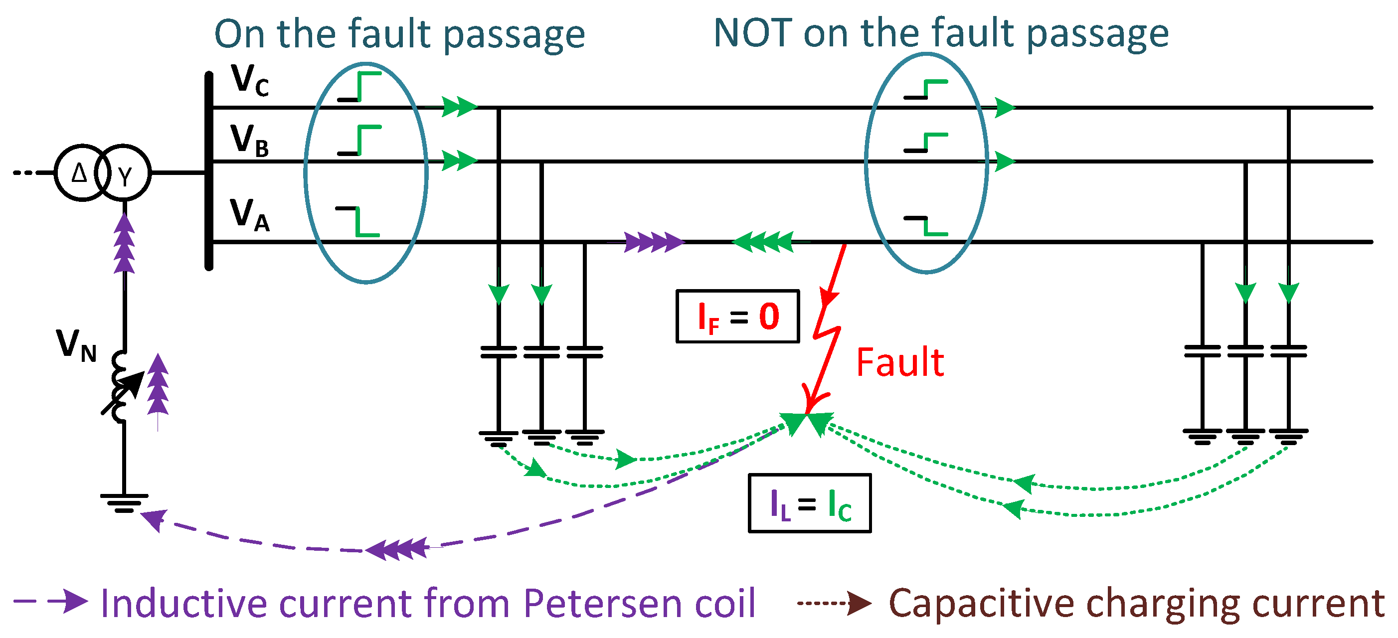
In a symmetric three-phase network with resonant earthing, the potential of the transformer neutrality during balanced conditions is equal to the earth potential. During an earth fault, this potential changes, depending on the fault’s resistance. For a metallic earth fault, the voltage of the faulty phase becomes almost zero. All potentials in the network shift by approximately this same phasor change because the currents caused by the earth fault are not high enough to cause large voltage drops in the network impedances. The change in the faulty-phase potential therefore appears between the neutral and earth in the opposite direction, driving a current through the coil.

Figure 1 shows the current distribution during an earth fault in a resonant earthed system when the Petersen coil is tuned to the resonant point.

The coil’s inductance at the resonant point can be expressed in terms of the system’s angular frequency $\omega$ and phase-to-earth capacitance C, as

$$L=\frac{1}{3{\omega }^{2}C}$$

(1)

In this simple model with a symmetric network, no series impedance in the lines, purely capacitive shunt admittance, and no resistance in the coil, the fault current $i_{\mathrm{F}}$ through the fault location is zero when (1) is fulfilled.

In a balanced operation, the phase quantities are separated by ${120}^{\circ }$. If E is the phase-voltage magnitude, and $\alpha =1\angle {120}^{\circ }$, then with phase-A potential as the reference angle, the phase potentials and currents can be expressed in the following way, where the appended subscript ‘1’ denotes the initial, no-fault case:

$$\begin{array}{cc}\hfill v_{\mathrm{A}1}=E,& i_{\mathrm{A}1}=j\omega CE\hfill \\ \hfill v_{\mathrm{B}1}={\alpha }^{2}E,& i_{\mathrm{B}1}={\alpha }^{2}j\omega CE\hfill \\ \hfill v_{\mathrm{C}1}=\alpha E,& i_{\mathrm{C}1}=\alpha j\omega CE\hfill \end{array}$$

(2)

Consider a solid earth fault on phase A. The currents involved are only of the level of load currents or lower, so the source continues to maintain the usual voltages between phase conductors and the source neutral. The fault makes the potential of the faulted phase-conductor, relative to earth, change from phasor E to 0. All the other potentials in the system are therefore shifted by this same phasor change to become

$$\begin{array}{cc}\hfill v_{\mathrm{N}2}& =-E\hfill \\ \hfill v_{\mathrm{A}2}& =0\hfill \\ \hfill v_{\mathrm{B}2}& ={\alpha }^{2}E+v_{\mathrm{N}2}=({\alpha }^2-1)E\hfill \\ \hfill v_{\mathrm{C}2}& =\alpha E+v_{\mathrm{N}2}=(\alpha -1)E\hfill \end{array}$$

(3)

The capacitance of the faulted phase to earth therefore completely discharges, while the capacitances of the healthy phases to earth charge further due to the potential rise of the healthy phases. The changes in the phase currents due to the earth fault are then

$$\begin{array}{cc}\hfill \Delta i_{\mathrm{A}}& =i_{\mathrm{A}2}-i_{\mathrm{A}1}=j\omega C\left(v_{\mathrm{A}2}-v_{\mathrm{A}1}\right)=j\omega CE(0-1)=-j\omega CE\hfill \\ \hfill \Delta i_{\mathrm{B}}& =i_{\mathrm{B}2}-i_{\mathrm{B}1}=j\omega C\left(v_{\mathrm{B}2}-v_{\mathrm{B}1}\right)=j\omega CE({\alpha }^2-1-{\alpha }^2)=-j\omega CE\hfill \\ \hfill \Delta i_{\mathrm{C}}& =i_{\mathrm{C}2}-i_{\mathrm{C}1}=j\omega C\left(v_{\mathrm{C}2}-v_{\mathrm{C}1}\right)=j\omega CE(\alpha -1-\alpha )=-j\omega CE.\hfill \end{array}$$

(4)

This shows that the phasor changes in the phase currents due to a metallic earth fault are equal:

$$\Delta i_{\mathrm{A}}=\Delta i_{\mathrm{B}}=\Delta i_{\mathrm{C}}\mathrm{and}\mathrm{therefore}\mathrm{also}|\Delta i_{\mathrm{A}}|=|\Delta i_{\mathrm{B}}|=|\Delta i_{\mathrm{C}}|.$$

(5)

Equation (5) is also valid for resistive earth faults in the simple model of Figure 1, as long as the Petersen coil is tuned to the resonant point. In this condition, the magnitudes of changes in the phase currents have a similar nature regardless of whether the measurement point is on the fault passage or not.

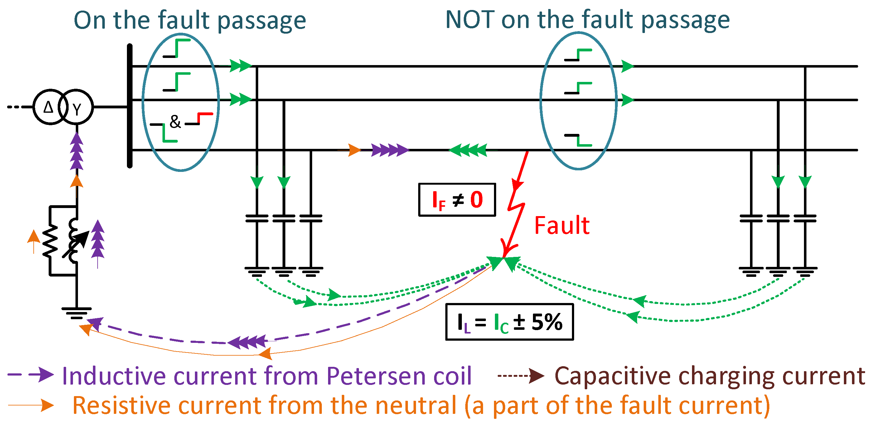
Real distribution networks are usually not transposed, so asymmetries exist during normal operation, particularly with open-wire overhead lines. The transformer neutral’s potential, $v_{\mathrm{N}}$, in an unfaulted operation is then not equal to the earth’s potential. If the coil is tuned to the resonant point, $v_{\mathrm{N}}$ will be very sensitive to any unbalance, reaching high levels in normal operation. This is one reason why resonant earthed networks are seldom operated at the resonant point [20]. The usual practice is to run the network in a slightly over-compensated condition [21], meaning that the coil produces somewhat more current than is needed to cancel the capacitive current. This additional current can pass through an earth fault. Figure 2 shows the situation of an earth fault in an over-compensated network.

In some cases, there is a resistance connected in parallel with the Petersen coil to assist the protection systems in finding the faulty feeder [22] and to subdue the rise in neutral voltage due to natural asymmetries. The maximum fault current through the fault location can be controlled by the choice of resistance and the degree of over-compensation.

The fault current flows through the faulty phase and returns through the fault location. Hence, at points on the fault passage from source to fault, the change in the current magnitude of the faulty phase is not equal to the changes in the current magnitudes of healthy phases. Anywhere else in the network, not on the fault passage, Equation (5) remains valid.

In a real system, the lines will carry the load current as well as the currents due to system capacitance and the fault. A steady load is negligible for the above analysis because phasor-changes in the phase currents ($\Delta i$) are considered, based on ideal measurements. However, large changes in load during the fault would create a risk of affecting the detection result by introducing another cause of $\Delta i$. This is treated further in the Discussion.

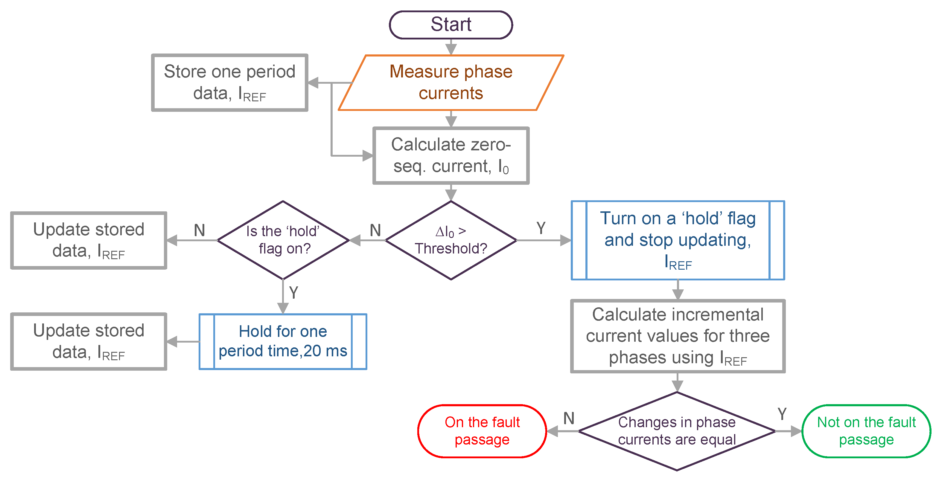
3. Proposed Algorithm

Figure 3 shows the flow chart of the proposed algorithm to identify the fault passage. The algorithm continuously samples the phase currents, calculates the zero-sequence currents and stores one-cycle phasor data of the latest cycle. If the change in the zero-sequence current is above a preset threshold, the algorithm infers a fault condition and holds the stored phasors without updating them.

The later cycles of phase currents are then compared with the stored cycle to find the changes in the phase currents. If the magnitudes of these phasor changes in phase currents are similar for all three phases, the location of that measurement is reported as not being on the fault passage; otherwise, the location is reported as being on the fault passage. In practice, the changes in the healthy phases are not expected to be precisely equal, due to factors such as measurement errors or natural unbalances in the network. However, the distinguishing gap between the changes in the faulty phase and healthy phases is seen by the simulation to exist despite reasonable levels of these disturbing factors.

The stored cycle should not be held for comparisons with cycles coming much later, e.g., multiple seconds between the compared cycles. One reason is that the correct comparison of the phase angle between widely separated cycles, without a further synchronizing signal such as a system voltage, is sensitive to disturbance from frequency deviations, as taken up further in the Discussion. After a reasonable time for making an FPI decision, such as 0.1 s after fault inception, the stored cycle can again start to be refreshed in a practical implementation. However, in the plotted simulation results, a longer time is used to show the long-term development of the measured quantities; there is no issue with frequency, as the simulation has a known frequency and a suitable sample rate.

The phasors are derived by discrete Fourier transform (DFT) on one-cycle windows of samples to find the fundamental frequency component’s magnitude and phase. For the chosen sample rate of 1 kHz, there are 20 samples in a one-cycle window for the network’s 50 Hz nominal frequency. The phasor angles are defined relative to the first point in the one-cycle window. In order to have the pre-fault and post-fault phasors using the same angle reference, the time between their two windows is chosen as a whole number of periods, i.e., a multiple of 20. This assumes that the network is at its nominal frequency. The assumption is true for the simulated data, but there could be a deviation in a real system, as is taken up further in the Discussion.

4. Test-Network Description

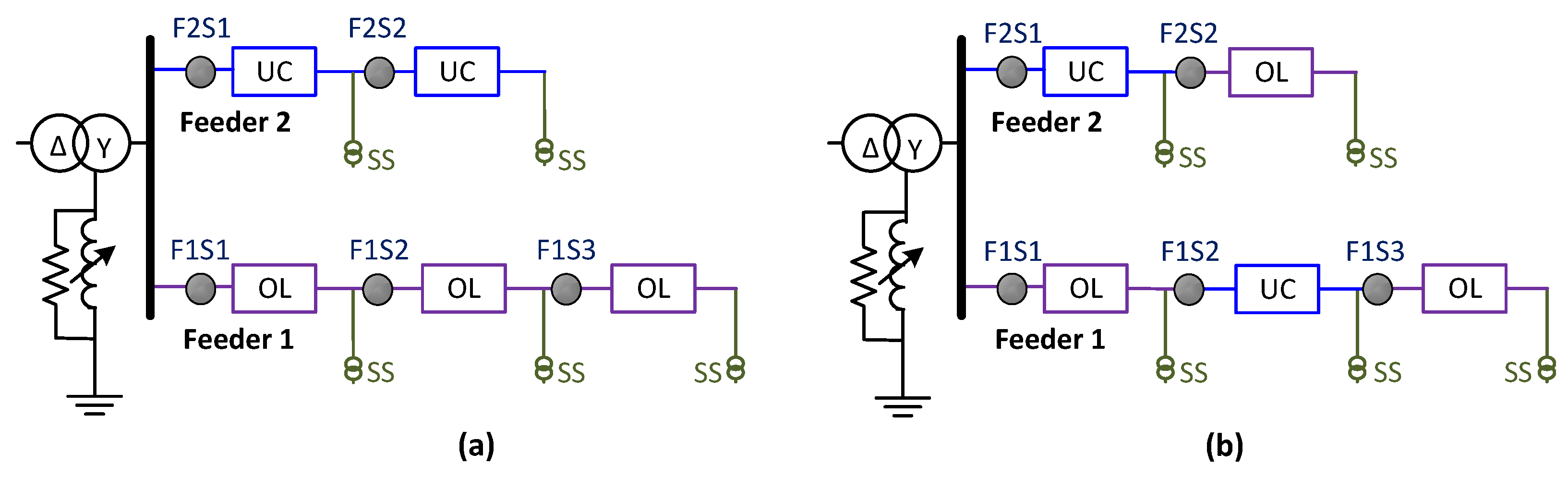
The proposed method was tested by implementing it in Matlab, and running this with input from time-domain simulations in PSCAD of various resonant earthed networks. Results presented here are based on the two networks shown in Figure 4.

The first has homogeneous feeders, i.e., feeders that contain either entirely overhead lines or entirely underground cables. The second has mixed (heterogeneous) feeders, containing both overhead lines and underground cables. Each of these shown networks has two feeders. F1S1, F1S2, and F1S3 are locations of FPIs in feeder 1, at the beginning of feeder sections 1–3 respectively. Locations F2S1 and F2S2 are named similarly for the second feeder.

These test networks were chosen from a wider range of simulated networks as giving a clear demonstration of the performance of the proposed method in various scenarios. The method was also tested for feeders with several branches, which were found to have a negligible impact beyond what can be seen from the two networks of Figure 4 when looking at the different FPI locations with various combinations of line and cable in the five sections of the two feeders. For both of the networks, the nominal line-voltage is 22 kV, and the total connected load is about 7.025 MW (power factor 0.9 lagging), distributed between the five secondary substations (SS). The Petersen coil is tuned for 10 A over-compensation, and a resistor in parallel with the coil provides 3 A when subjected to the system’s rated phase-voltage.

For the network with homogeneous feeders, Feeder 1 is 30 km long with section lengths of 10.5 km, 16.5 km and 3 km. Feeder 2 is 20 km long with two equal sections of 10 km. For the network with mixed feeders, the difference compared to the homogeneous network is simply that the second section of each of the feeders is swapped. Hence, the homogeneous and mixed networks both have the same capacitive charging current, which is 56 A.

The PSCAD implementation uses the $\Pi$-section line model. This is simple but sufficient, as the proposed method uses fundamental frequency phasors, and the lengths of the sections are electrically very short for this frequency. The simulations were run with a solution time step of 50 $\mathsf{\mu }$s. However, in order to represent a simple measurement system, current values sampled at just 1 kHz were recorded from the mentioned FPI locations for further analysis in Matlab. The parameters of the overhead lines and cables are shown in

Table 1. Network parameters.

Type		Resistance	Inductance	Capacitance
		($\mathbf{\Omega }$/km)	(mH/km)	(nF/km)
Cables	+ve seq.	0.319	0.37	219.9
	zero seq.	1.258	5.1	219.7
Line	+ve seq.	0.21	1.1	11.05
	zero seq	0.67	4.8	3.95

, and are based on values used for this type of study by a sponsoring utility.

5. Results

This section describes tests of the proposed method’s operation in several simulated cases. Locations on and off the fault passage are tested, as either a false-positive or false-negative result from an FPI is likely to increase the time taken to locate the fault. When using FPIs, the section that will be considered to be faulty is delimited by at the upstream end by the last FPI that reports a fault passage (or by the source substation) and at the downstream end by the first FPI that does not (or by the end of the line). A wrong result from one FPI could in some cases cause the wrong section of line to be searched.

The following subsections show a figure for each presented test. Each figure has subplots for the five tested FPI locations in the studied network. Each subplot has one curve per phase, marked $|\Delta i_x|$, which is the magnitude of the phasor change of current in phase-x. With the chosen 1 kHz sample frequency, there is one point per millisecond. The value plotted at each time point is based on the fundamental component of the DFT of 1 cycle (20 measurement samples) ending at that point, minus the DFT of the selected pre-fault cycle. When there is not a whole number of cycles between these two compared cycles, an appropriate angle-shift is applied to obtain the correct phase difference.

If not mentioned otherwise, the system is 10 A over-compensated, and the resistance in the neutral in parallel with the Petersen coil is selected to provide a maximum of 3 A resistive current.

5.1. Performance for Different Network Types: Line, Cable, Mixed

Traditionally, distribution feeders tended to be either open-wire overhead lines or underground cables, with little or no mixture. Overhead lines are common in rural networks, whereas cables are common in urban areas. The number of mixed feeders with significant proportions of both overhead lines and cables is increasing, especially in the Nordic countries. A major driver for this is the demand for increased reliability of rural networks in bad weather. This has led to more underground cables replacing overhead lines. It has also become common in heavily wooded areas to use aerial insulated cables instead of open-wire lines to increase reliability while keeping the line visible and avoiding digging.

Underground or aerial cables increase the charging capacitance many times compared to open-wire lines, as is clear from Table 1. For a homogeneous feeder, the relation between magnitudes of capacitive currents and load current is therefore very different for cables in comparison to lines. It is important to check the robustness of the proposed method for the different types of network feeders with their different capacitances, and also for mixtures.

5.1.1. Networks with Homogeneous Feeders

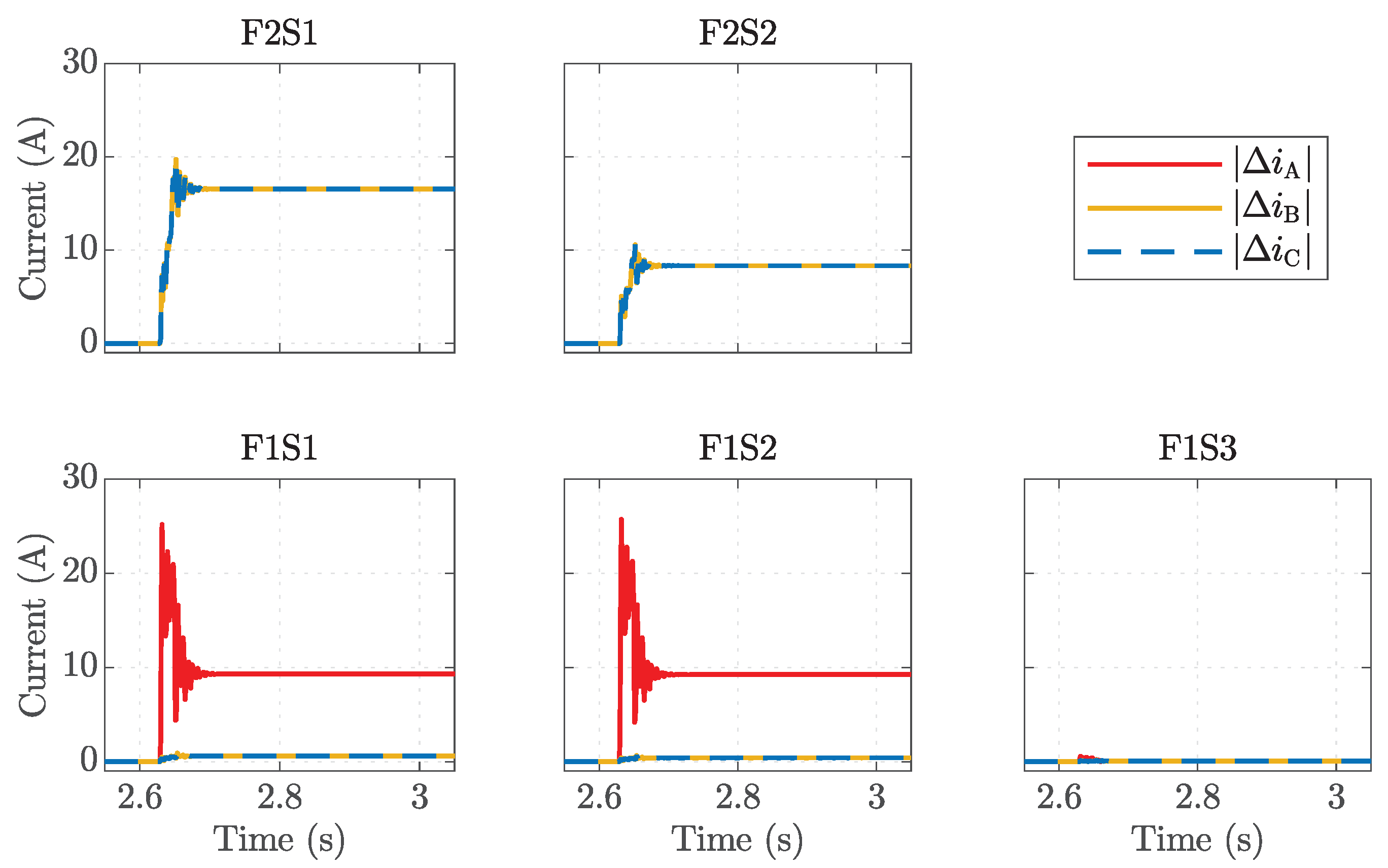
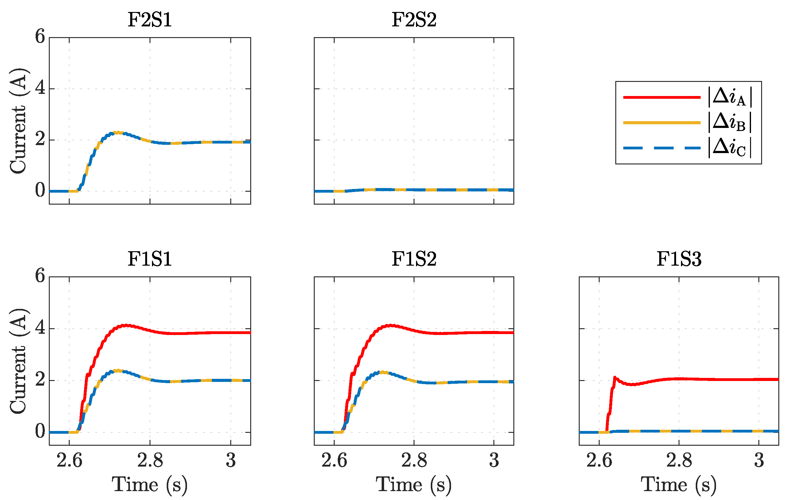
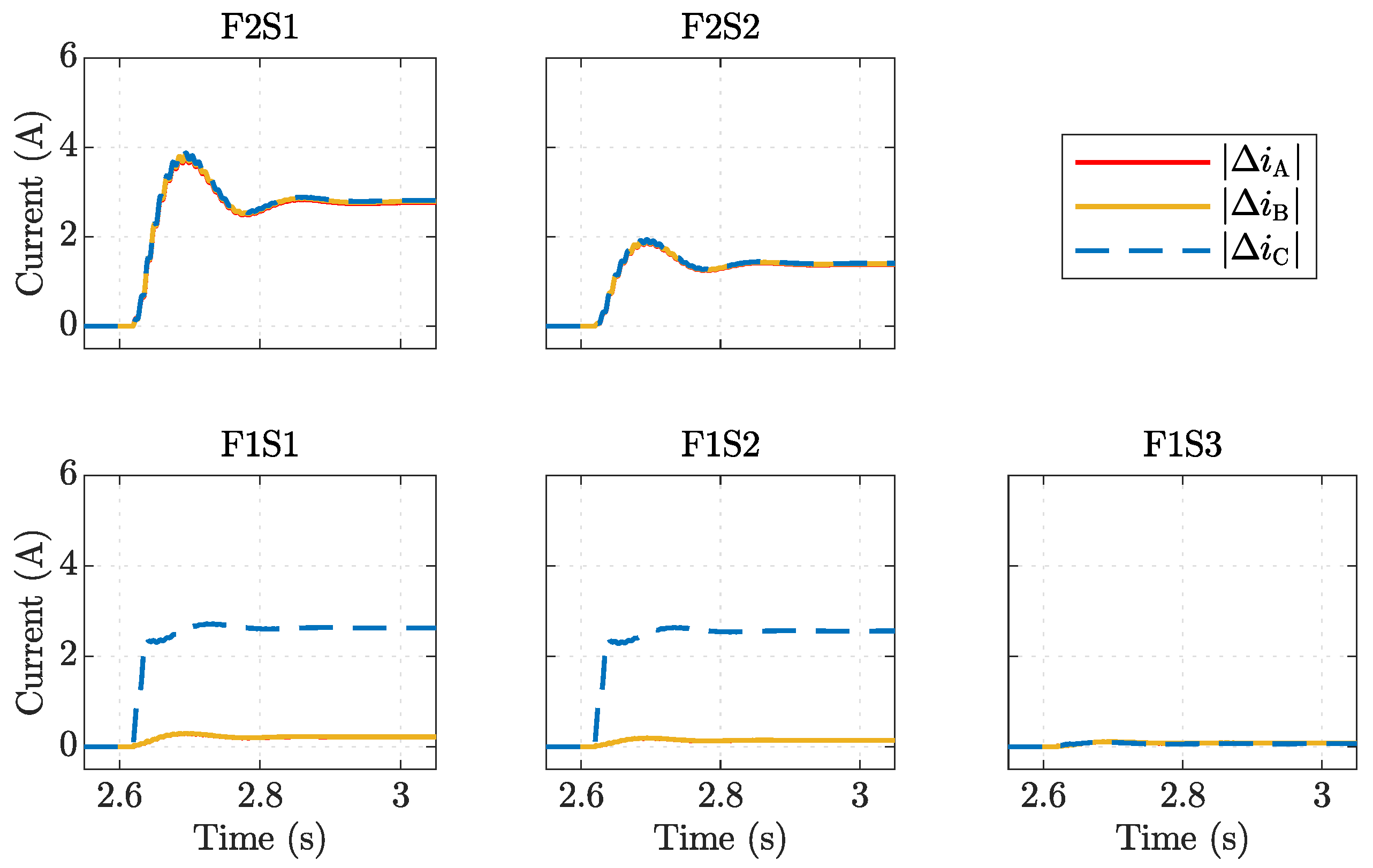
The network shown in Figure 4a is used here as an example with homogeneous feeders. Figure 5 shows the results for a solid earth fault in the middle of the second section of the feeder with overhead lines, between F1S2 and F1S3.

The fault occurs at 2.61 s, and the changes in current magnitudes of the three phases are the same for the FPIs in feeder 2 (F2S1 and F2S2). In contrast, for feeder 1, the changes in current magnitudes are not the same for feeder sections 1 and 2, but they are for feeder section 3. The fault is therefore deduced to be in feeder section 2 since F1S3 is located at the beginning of feeder section 3. The magnitudes of changes in the healthy-phase currents are smaller in feeder 1 than in feeder 2 because feeder 2 contains cables.

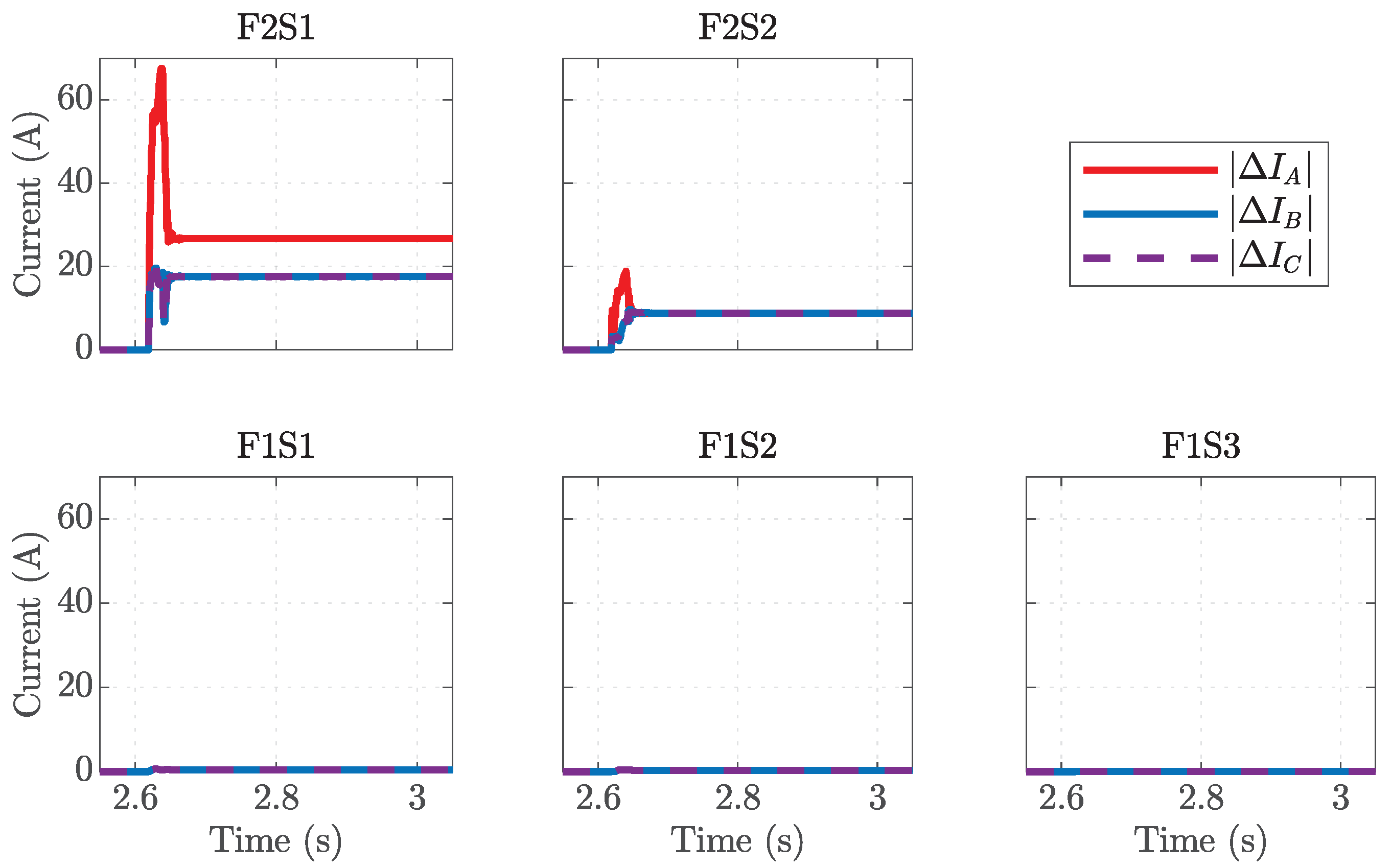
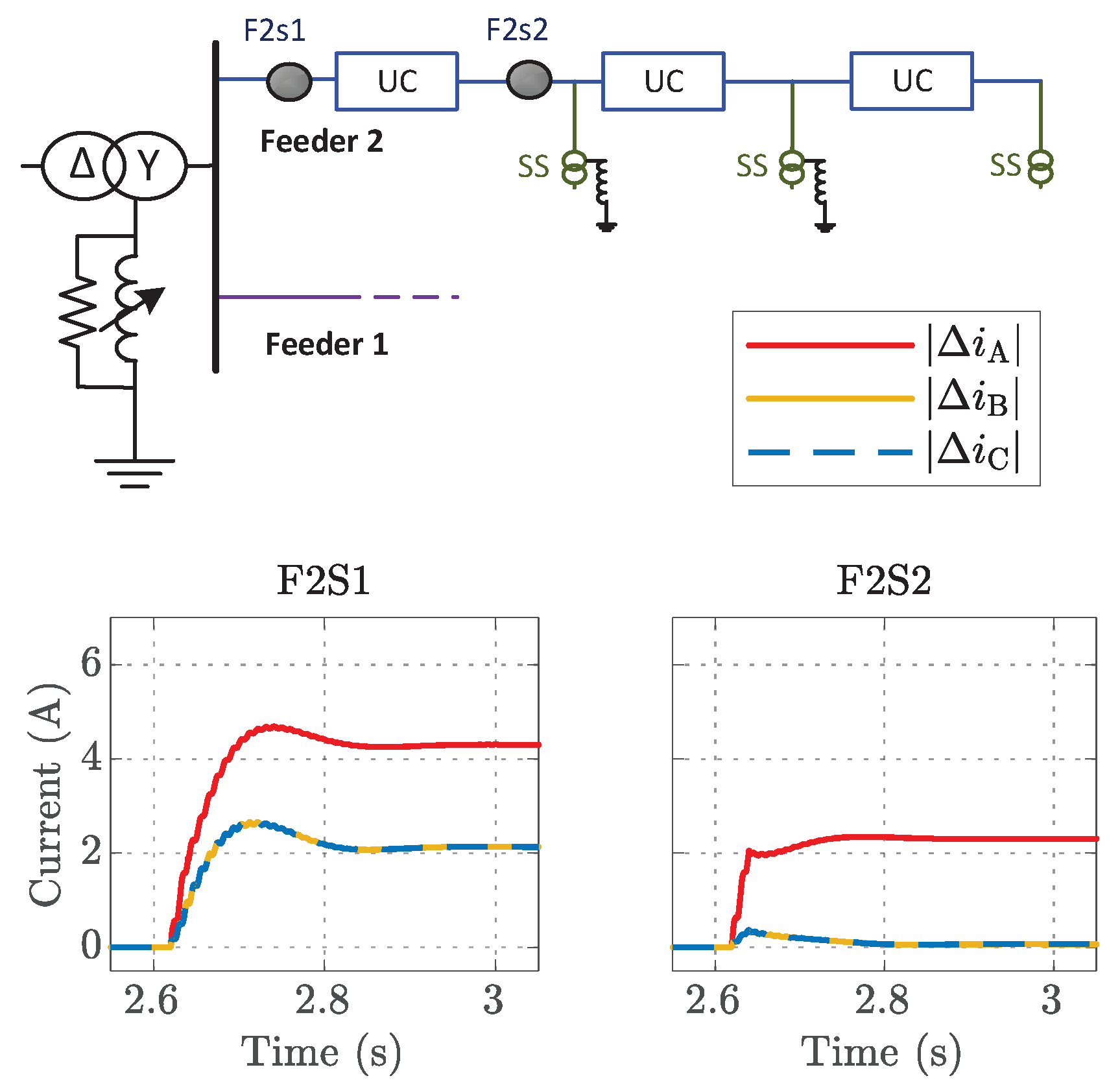
For the same network, Figure 6 shows the result when a solid fault is applied in the first section of feeder 2, which consists of cables. The changes in current magnitudes are not visible for feeder 1 since all the vertical axes are scaled to be consistent and to accommodate the values for feeder 2. The changes for F2S1 are not the same throughout the whole duration. However, for F2S2 the changes are not the same right after the fault inception but then they become the same. Therefore, the proposed method should not be decided on based on the information from the transient period. The sampling frequency used in the analyses is 1 kHz, which is not sufficient to provide reliable information during the transient periods.

5.1.2. Networks with Mixed Feeders

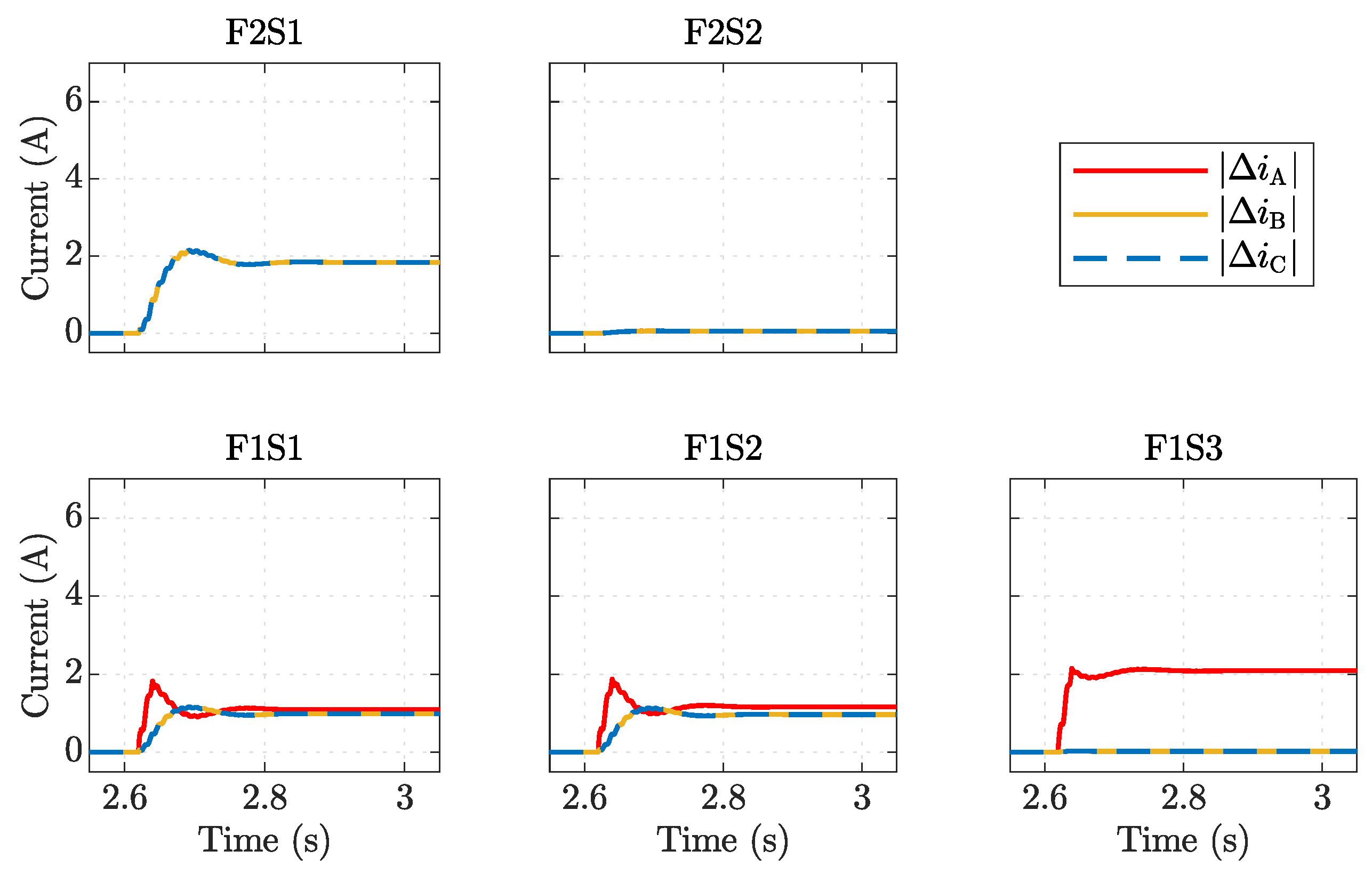
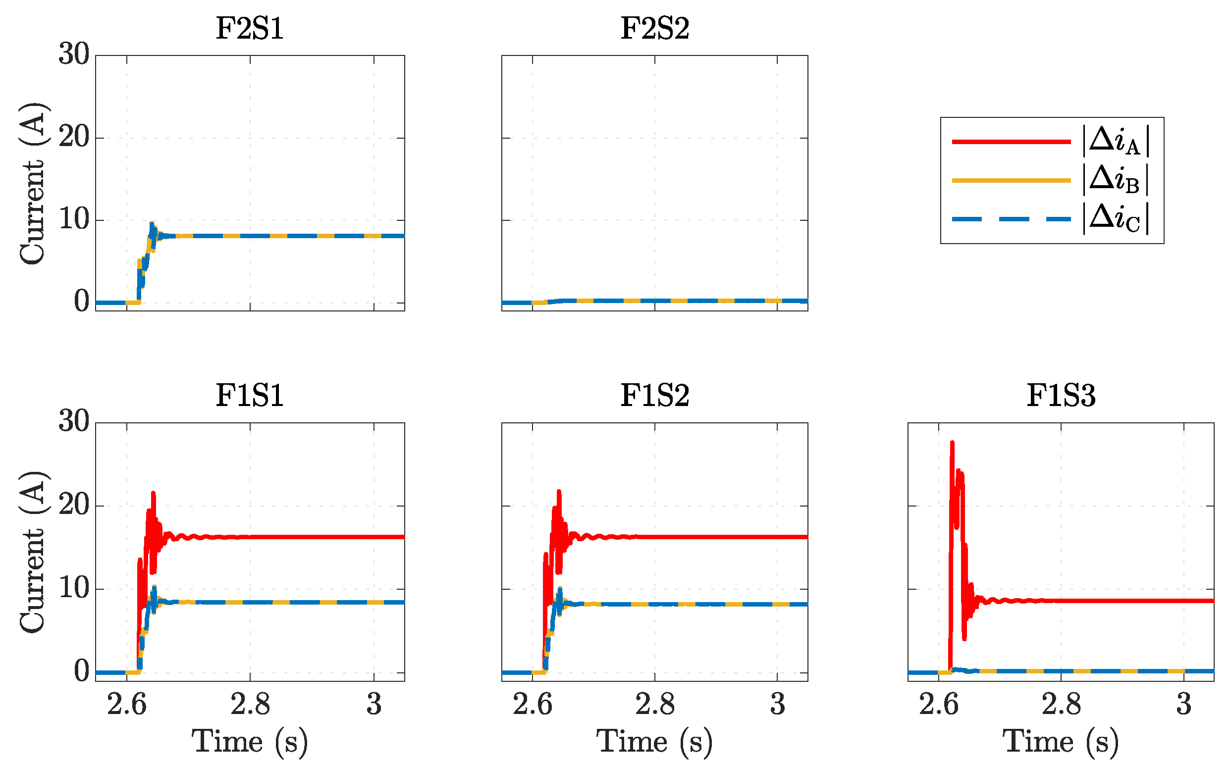
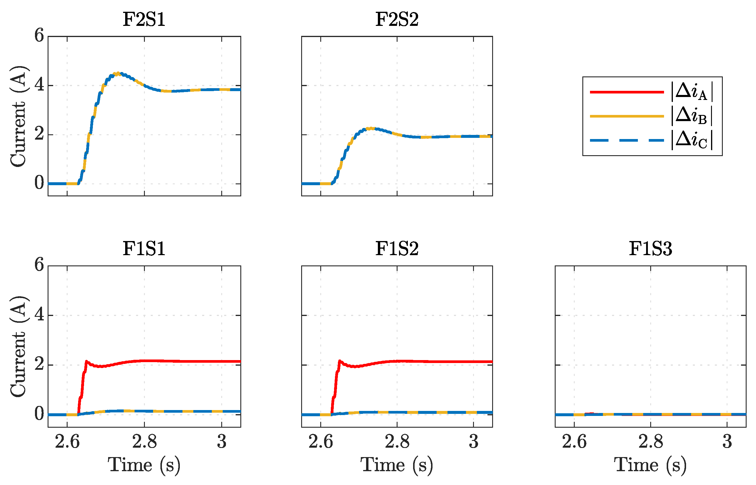
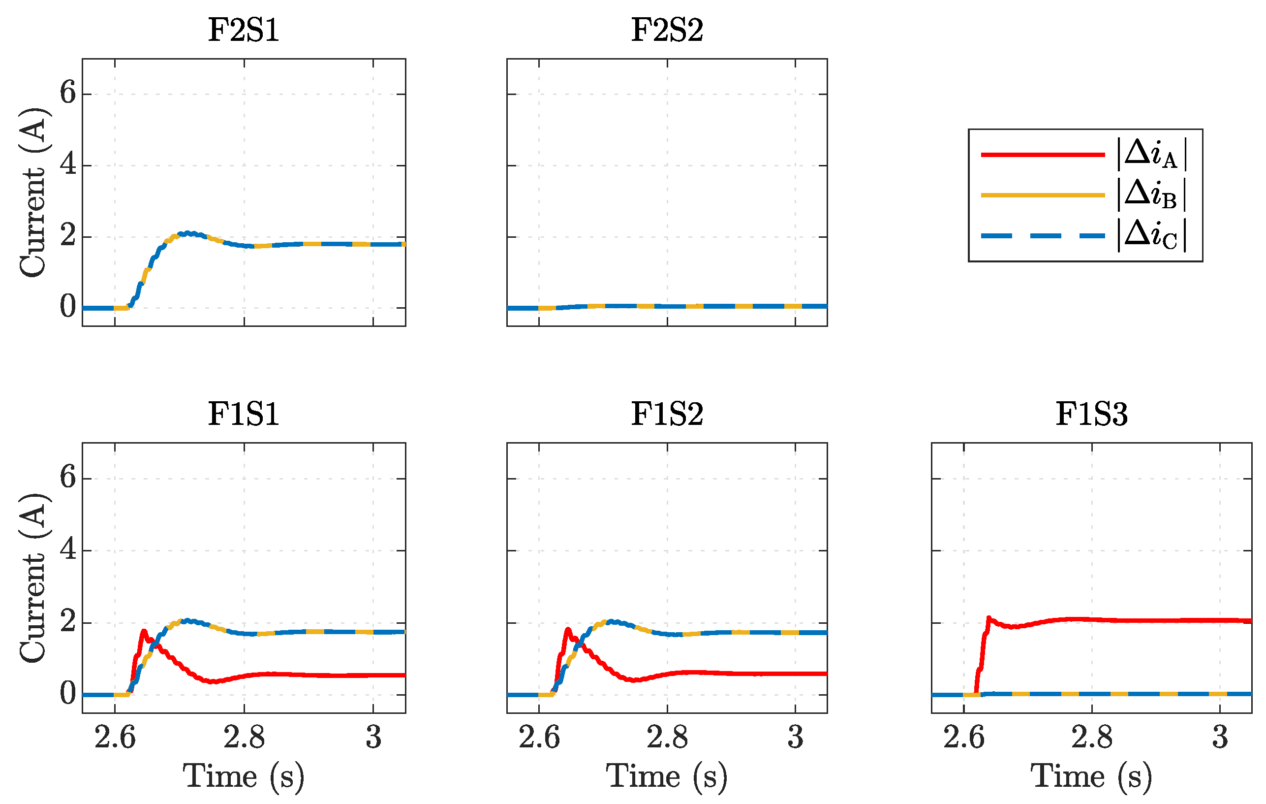
The network shown in Figure 4b is used to check the performance of the proposed method in mixed feeders. The third section of feeder 1 contains overhead lines. Figure 7 shows the results for a solid earth fault on an overhead line in the end section of feeder 1. For all the FPIs in feeder 1, the magnitudes of current change are not similar between the phases. This suggests that the fault is in feeder section 3, between the last FPI (F1S3) and the end of the network.

Although the first section of feeder 1 contains overhead lines, the capacitive current flowing through it is high because the second section consists of cables. The third section is the last part of the feeder, and it contains overhead lines. Therefore, the changes for the healthy phases are greater for F1S1 and F1S2 compared to F1S3. For the second feeder, changes in the first section are greater than that in the second section because the first section of this feeder contains cables whereas the second section contains overhead lines. However, for both sections, the magnitudes of the changes in all phase currents are almost the same since feeder 2 belongs to the healthy part of the network.

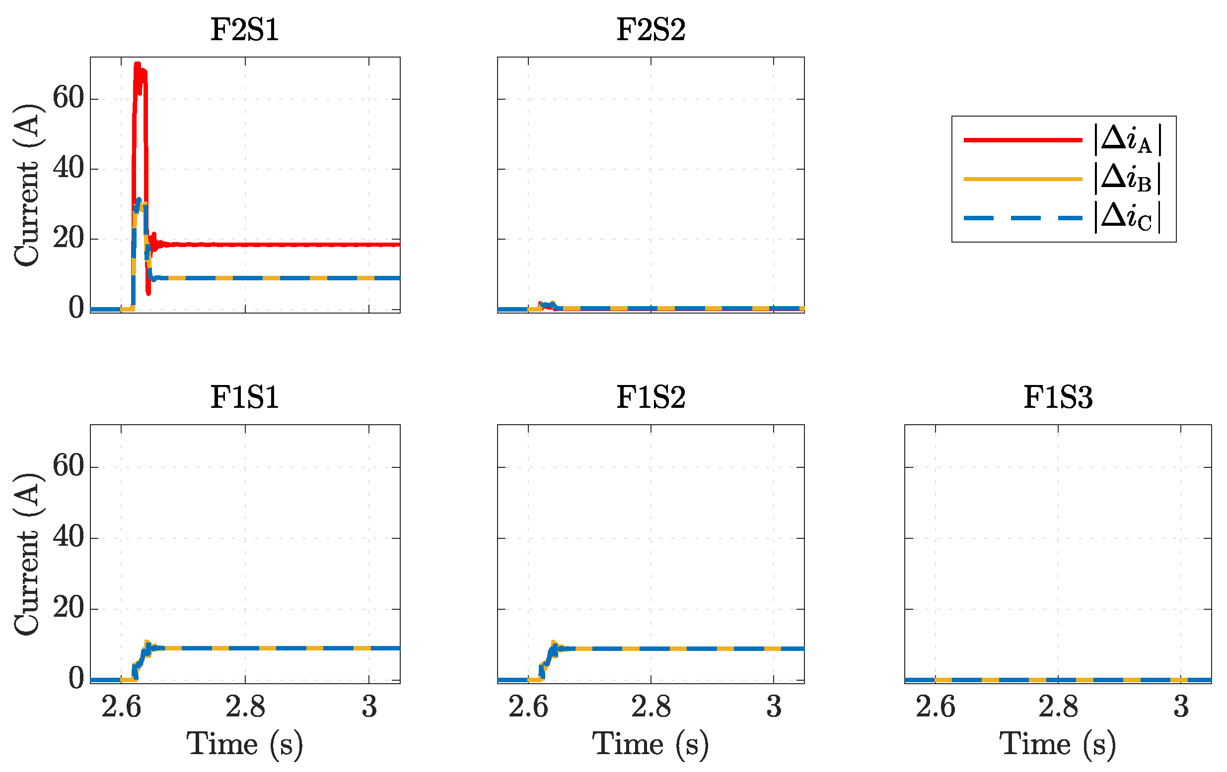
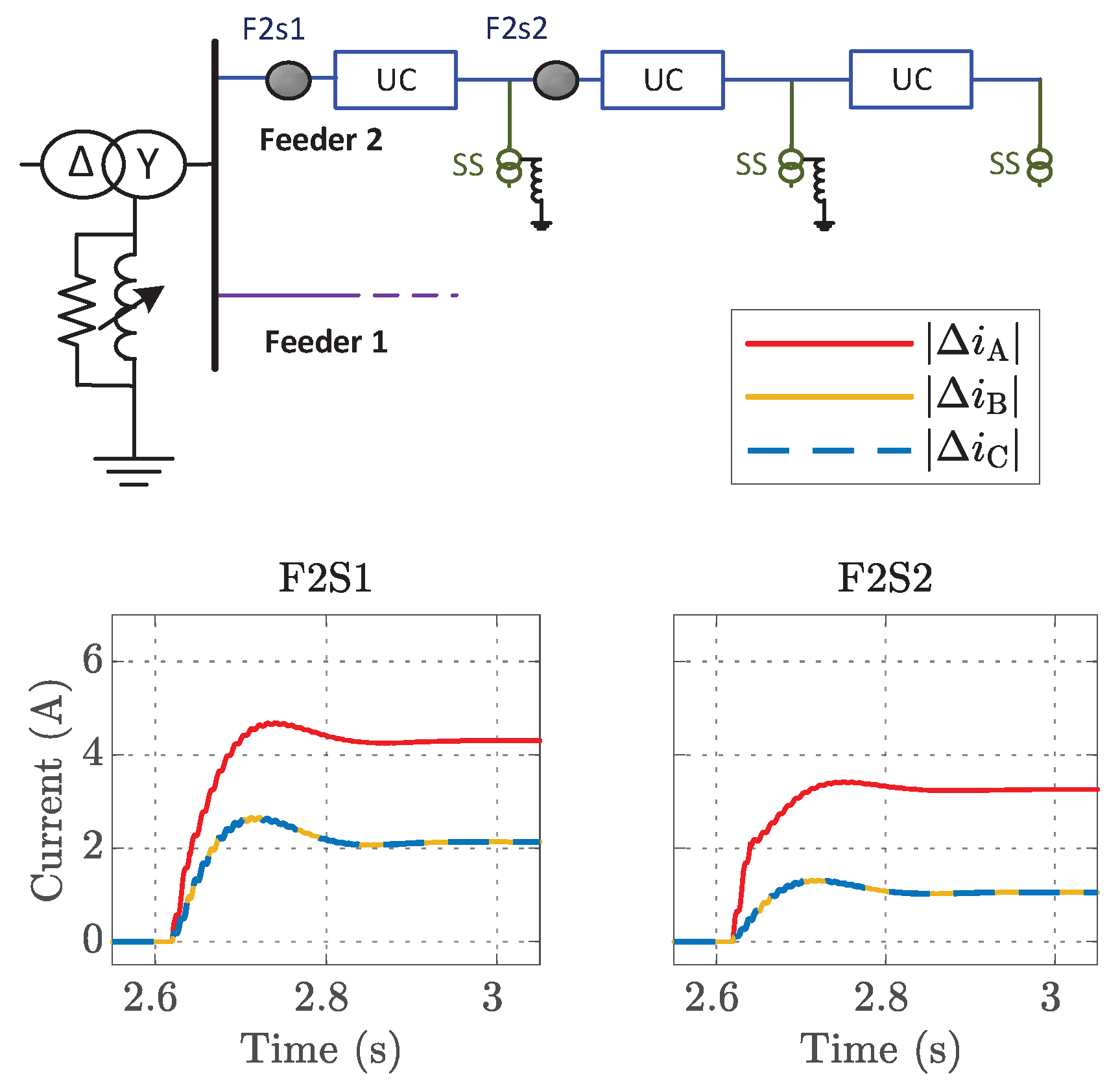
Figure 8 shows the results for a solid earth fault in the first section of feeder 2. This section contains cables in that mixed feeder. The change in the healthy phase currents is almost similar to the case with a fault in feeder 1 (Figure 7). This characteristic shows that the changes in the healthy phases are primarily due to the quantity of charging current flowing through a location of a feeder during the fault. However, the magnitude of change for the faulty phase current is higher than that for the healthy phases for F2S1 but not for F2S2. It indicates that the fault lies between these two measurement points.

5.2. Impacts of Fault Resistance

Most of the faults in distribution systems involve resistances of various magnitudes. It is important that the system can identify the resistive faults to ensure safety in the surroundings of the earth fault location. In Sweden, earth faults of up to 5 k$\Omega$ fault resistance must be identified and automatically cleared within 5 s if any part of the network contains overhead lines. Any persistent fault up to this resistance therefore would require that the fault is found and repaired in order to be able to restore all customers. The proposed method is, therefore, tested, even for 5 k$\Omega$ fault resistances in mixed feeders.

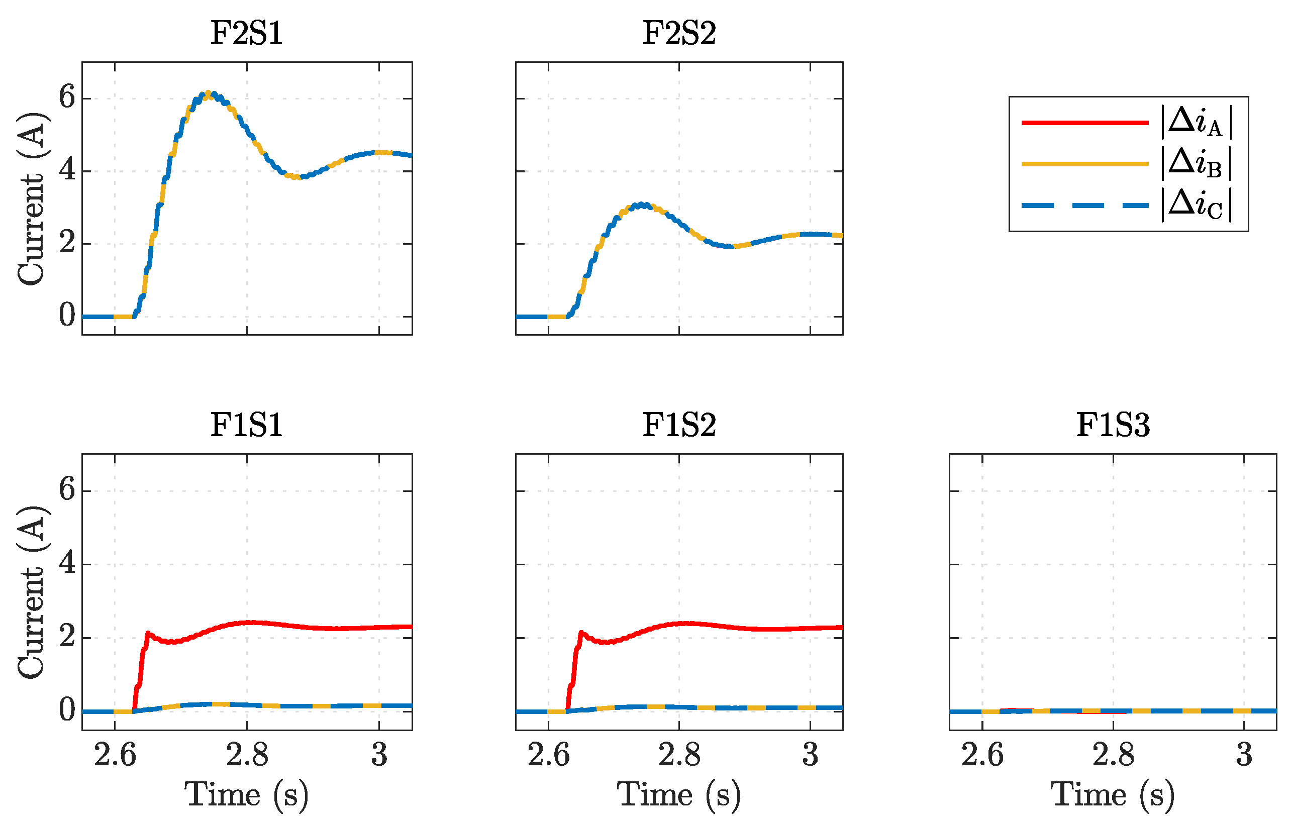
Figure 9 shows the results for a 5 k$\Omega$ earth fault in the third section of feeder 1, which is a part of the mixed feeder with overhead lines. In order to observe the impact of the fault resistance, this figure can be compared with Figure 7 (solid fault), as all other details are the same between these two cases. The magnitude of the highest change has reduced from about 28 A to 4 A. The difference between the changes of the healthy phases and that of the faulty phase also reduced from about 18 A to about 2 A. This reduction can act as a deciding factor of the sensitivity of the proposed method. For example, changes of load during the few cycles after the fault inception will more easily disturb the FPI decision if the change that the FPI is looking for is weak.

5.3. Dependency on Resistive Current in the Neutral

A resistance in parallel with the Petersen coil can be used in various ways. A high resistance giving just a few amps of resistive current can be left normally connected. This helps restrict the neutral displacement during normal operation and enables the use of the watt-metric method by protection systems for identifying the faulty feeder. In some countries, a much lower resistance may be connected after a persistent fault is detected to enable the operation of fuses or simple fault location. In Sweden, the practice is to use only a high resistance, which remains connected during normal operation and during faults.

The effect of the resistive current is shown here for the network with homogeneous feeders, with a 5 k$\Omega$ fault resistance in the overhead-line feeder, between F1S2 and F1S3. Figure 10 shows the case with a neutral resistor in parallel with the coil, set to contribute 3 A resistive current in a solid earth fault; this was the situation for the earlier studied cases too.

Figure 11 differs only in that the neutral resistor is not present. The fault current reaches the steady state earlier when the resistor is connected at the neutral. The faulty section can be determined by the proposed method in both cases: with and without the resistor. Hence, unlike the watt-metric method, the method is not dependent on the resistive current from the system’s earthing, besides not requiring a voltage measurement.

5.4. Impact of Natural Unbalances in the Networks

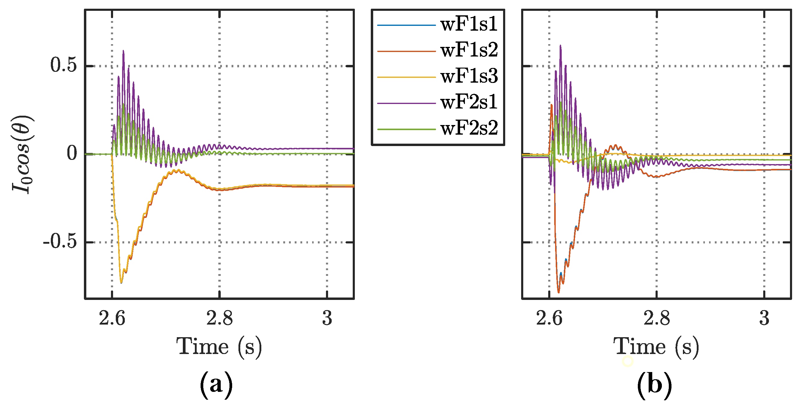
Asymmetries exist during normal operations in the distribution systems and thus displacements in the neutral voltage. This has an impact on the angle of the zero sequence voltage during fault conditions. The watt-metric method may become insufficient to distinguish between the faulty and healthy parts of the systems if the asymmetries are large enough. Figure 12 shows one such condition.

The vertical axes show the resistive part of the zero sequence current, $I_{0}cos\left(\theta \right)$ where $I_0$ is the magnitude of the zero sequence current and $\theta$ is the angle between zero sequence voltage and the zeros sequence current. To simulate the natural unbalanced condition, the capacitance of phase A is increased, and phase C is decreased by 1% from the balanced condition. The results in Figure 13 are for the same conditions as for Figure 12b, and it shows that the proposed method is not severely impacted by network asymmetry.

5.5. Impact of the Network’s Compensation Location and Degree

The foregoing tests considered one level of over-compensation, with the compensation provided entirely at the neutral of a single transformer that supplies the network. The following tests consider some differing cases of practical relevance.

5.5.1. Distributed Compensation

Distributed compensation splits the compensation inductance between different points in the network. A typical implementation is that one tunable central coil compensates for part of the network and adjusts the compensation degree, while several earthed zig-zag transformer windings with fixed values are spread throughout the system to locally compensate for outlying parts of the network. This distributed approach was described even in Petersen’s patent [1], but its uptake in Sweden has been driven more recently by the move to using cables to replace even long rural lines [23]. Previously, the cable networks were in urban areas, where the high load density restricts the total length of cable that will be found in a network. Distributed compensation is a better choice for the networks that have long feeders with cables, where the series resistance becomes significant as a proportion of the shunt capacitive reactance.

Feeder 2 of the network presented in Figure 4a is used as an example. The first section and feeder 1 are compensated for by the central coil, whereas the second section is divided into two equal parts and compensated for with two local compensation coils of the same size. This arrangement is shown in Figure 14 and Figure 15. The fault is between F2S2 and the end of the feeder, and has a resistance of 5 k$\Omega$.

Figure 14 shows the results when the placement of F2S2 is before these two compensation coils. The changes for the healthy phases are moderate because the capacitive currents for the remaining part of the feeder do not cross this location.

Figure 15 shows the case when the placement of F2S2 is just after one of these two local compensating coils. Now, capacitive currents of 5 km of cables pass through F2S2, so the changes for the healthy phases are almost half compared to that for F2S1. The proposed method shows satisfactory results in both conditions.

5.5.2. Under-Compensation

Although resonant earthed systems are most commonly run in compensated conditions, a few are run in under-compensated conditions [21]. The network can become under-compensated due to failures in the tuning mechanism of the Petersen coil, or failure of any of the distributed coils in the case of distributed compensation.

It is therefore of interest to test the method’s performance with under-compensation, although this is not as important as over-compensation. For this purpose, the mixed network (with purely central compensation) is tuned to 10 A under-compensation, and faults are applied in different feeder sections.

Figure 16 shows the results when 5 k$\Omega$ fault resistance is applied after F1S3. The changes in the current magnitudes are not the same on the fault passage, but the change for the faulty phase is smaller than that of the healthy phases. It is more prominent when Figure 16 is compared with Figure 9 since all other conditions are the same for these two cases, except the degree of compensation.

In this case, the network is under-compensated, so the fault current is capacitive. The change in the faulty-phase current due to an earth fault appears as inductive because it arises mainly from the reduction in the capacitive current. The fault current (capacitive) flowing from the start of the feeder is added with this reduced charging current (inductive) throughout the fault passage. As a result, the magnitude of the change in the faulty-phase current becomes smaller for under-compensated networks compared to over-compensated networks.

To demonstrate the impact of this feature, Figure 17 shows an example with 10 A under-compensation, implemented by reducing the length of the second section of feeder 1 from 10 km to 5.5 km to reduce the charging current. The method then does not determine F1S1 and F1S2 to be on the fault passage since the changes for the three phases are almost equal: this is a wrong decision. The changes for faulty and healthy phases can become equal, depending on the compensation degree and amount of charging current at an FPI’s location on the feeder.

Therefore, the proposed method is not well suited to under-compensated networks, which would require further investigation. This work focuses on over-compensated networks, which is a common situation in Sweden.

6. Discussion

Identification of the fault passage is challenging for resonant earthed systems because the magnitude of the fault current is fairly small even compared to load currents, and because zero sequence current flows throughout the whole system during an earth fault.

The proposed FPI method is aimed at simplicity and low cost by using only current measurements, at the one location, at the relatively low sample rate of 1 kHz. It also has no requirement on including or changing an earthing resistance during the fault. These points give the potential for lower cost than for several other approaches that were surveyed in Section 1.

The method showed good selectivity for over-compensated networks. However, it was shown to have reliability problems for systems with high capacitive currents, operated in under-compensated conditions. Looking into the changes in the angles instead of magnitudes may provide reliable results during these situations; further investigations can focus on this.

The test cases studied here had a fault implemented as a switched impedance. There have not been tests of faults that give sharp transients of current, such as an intermittent arcing fault.

In the test implementation with 50 Hz fundamental frequency and 1 kHz sampling frequency, phasors were calculated from windows of 20 sample points, i.e., 1 cycle. The windows used for calculating phasors from before and after the fault had their start-points separated by an integer multiple of the window length, in order to compare the phasors with correct relative angles. If the system frequency deviates from 50 Hz, a phase-error will arise in the comparison, proportional to the frequency deviation and the number of window-lengths of separation. How much this could affect the results depends partly on the load currents at the FPI location, as even a constant load will contribute to the phasor change between two measurements that have an erroneous relative shift in their relative phase. In a very large power system, such as the continental European system (usually controlled within $\pm 25$mHz), the frequency at almost all times, except short, extreme disturbances, gives only up to 1${}^{\circ }$ phase error when phasors are compared between times separated by two window lengths (40 ms). However, smaller systems have larger bands of normal variation: for example, some are 4 times as much in the Nordic synchronous system, and much smaller island systems are also to be found. A larger number of periods separating the compared windows might also be desired. Some mitigation is therefore advisable for robust practical implementations of the method. An example of a design mitigation is to measure the actual frequency continually, and based on this, to apply a phase compensation after performing the DFT, or adjust the sampling frequency in proportion to the system frequency.

The method is based on comparing phasors between different times before and after the occurrence of an earth-fault, denoted by subscripts 1 and 2 in Equation (4). If a significant change of load occurs in this same interval, the sensitivity of the method can be reduced from 5 k$\Omega$ fault resistance to a lower value depending on the magnitude, phase angle and phase balance of the change.

Regarding the above effects of off-nominal frequency and load changes, it should be remembered that FPIs are aimed at improving supply reliability in an economic way; they are not a critical protection function whose misoperation poses danger. An occasional bad result due to external disturbance sources may be preferable for cost/benefit compared to an alternative that avoids the infrequent problem at the expense of including more measurements or complexity.

7. Conclusions

Testing based on simulation results showed good prospects for the proposed method in networks operated in over-compensated conditions. The method is not reliable for under-compensated networks; further investigation is required focusing on this matter.

The method’s advantage compared to some other available FPI implementations is that it works with very minimal information input: just phase currents at the FPI location, sampled at 1 kHz. This is in contrast to methods that require a voltage measurement too, measurements from multiple locations, higher-frequency measurement of transients, or changes of neutral-earthing resistance.