Dynamic Regression Prediction Models for Customer Specific Electricity Consumption

Abstract

We have developed a conventional benchmark model for the prediction of two days of electricity consumption for industrial and institutional customers of an electricity provider. This task of predicting 96 values of 15 min of electricity consumption per day in one shot is successfully dealt with by a dynamic regression model that uses the Seasonal and Trend decomposition method (STL) for the estimation of the trend and the seasonal components based on (approximately) three years of real data. With the help of suitable R packages, our concept can also be applied to comparable problems in electricity consumption prediction.

1. Introduction

Energy demand forecasting is an important factor for the effective management and planning of power systems. The population growth, rising living standards, urbanization, technological developments and industrialization have steadily raised the energy demand across many countries [1]. For electricity providers and regulators, the accuracy of their forecasts is crucial, as an overestimation of the respective demands might cause an excessive production in energy, which generally is difficult and costly to store, or even a substantially wasted investment in the construction of abundant power facilities. On the other hand, an underestimation may result in a risky operation strategy and unmet demand, as well as an insufficient preparation of their spinning reserves, potentially causing the system to fail in a vulnerable region [2].

Nowadays, electricity demand is subject to a wide variety of exogenous variables, including prevailing weather conditions, calendar effects, demographic and economic variables, as well as the general randomness inherent in individual needs. The effective integration of said factors into the forecasting methods in order to accurately meet the demand load has always been a challenge for modern power industries [2]. However, sometimes the only available information for the prediction are past consumption data from individual customers. This prediction challenge can then only be overcome with sophisticated prediction methods.

Since the forecasting of electricity demand is a classical problem, many forecasting models have been developed. Traditional forecasting models are frequently used for such problems, for example linear regression models, stochastic processes models, exponential smoothing and ARIMA (AutoRegressive Integrated Moving Average) models [3,4,5]. Recently, artificial neural network-based models (ANN) have been used as alternative approaches for forecasting purposes as well, as they can potentially learn non-linear dependencies in the electricity demand time series and have performed fairly well [6,7,8]. Furthermore, other Machine Learnings (ML) techniques such as Deep Convolution Neural Network (CNN), Support Vector Machine (SVM), Random forest algorithm were used to predict SARS-CoV-2 (COVID-19) based on symptoms and for discovering new candidate drugs and vaccines in silico diagnoses [9,10]. Among all forecasting algorithms that are being utilized for the prediction of future wind speeds, Support Vector Regression (SVR) and ANN are the most commonly used models [11].

There are rather few studies regarding forecasting methods for electricity consumption, where dynamic regression models are utilized in conjunction with the STL (Seasonal and Trend decomposition using Loess) decomposition method or where the Fourier series is applied in order to estimate seasonalities. Tarsitano and Amerise [12] have developed a new forecasting system for hourly electricity load in six Italian macro-regions. A seasonal autoregressive integrate moving average process (SARIMAX) with external variables as lagged hourly loads and calender effects together with a backward stepwise regression for parameter estimation was performed. Badri et al. [13] make a comparison between a variety of time series techniques, such as exponential smoothing, Box-Jenkins, and dynamic regression. Wang, Galjanic and Johnson [14] used a dynamic regression method and a two stage regression with ARMA (AutoRegressive Moving Average) model for predicting two day-ahead load electricity. Both models take into account temperature values, calendar effects, trend, seasonality and holiday components in the form of predictor variables. They have concluded that the dynamic regression model has the best performance overall compared to the alternative vendor developed models. Misha and Shaik [15] investigate the performance of a Prophet method with the Seasonality and Trend analysis with Loess (STL-ETS) method for electricity demand in regions of Texas. Tian et al. [16] combines the STL decomposition with GRU networks, where, firstly, a decomposition of the original data is performed via the STL method and the subsequent decomposed data are then imported into the main prediction module, which uses two GRU (Gated recurrent unit) networks with different structures to obtain the local and global dependencies of the data. Qiuyu et al. [17] decomposes the load using STL into two components, a base one which includes the trend and seasonality as well as a weather sensitive component. While the trend and seasonality is forecasted using the Holt-Winter method, a SVR model is trained by historical load data and meteorological data in forecasting the weather-sensitive component. Permata et al. [18] compare dynamic harmonic regression forecasting and its hybrid version involving calendar variation effects with double seasonal ARIMA (DSARIMA) for the electricity load.

The purpose of this study is to develop a benchmark model that captures the overall complexity of the electricity demand that a local electricity supplier faces on a daily basis. Here, we particularly focus on commercial customers that consume up to 100 MWh per year (the available data are provided by a local German electricity provider). We propose two dynamic regression approaches that differ mainly in their method for estimating the trend and seasonal components. Compared to other popular traditional time series models, these approaches are rarely investigated variants. The dynamic regression model makes use of the standard regression method to represent the relevant information from the independent variables (such as calendar variables or past consumption values) and an ARIMA model for the dynamic evolution of the error term to include the time series dynamics. In our first suggestion, we use Fourier series to model the seasonal periodicities, while the second technique uses the Seasonal and Trend decomposition using Loess method for estimating trend and seasonal effects.

Data sets of eight individual customers, which record the respective electricity consumption every fifteen minutes over the course of three years, have been provided by an electricity provider and will serve as the foundation for our research. Based on that, both of our proposed models will provide out-of sample forecasts for each data set. Specifically, we choose two-days ahead, seven-days ahead, and a month ahead as our forecasting horizons. Furthermore, the forecasting results of the electricity provider, that uses a variation of the average method, will serve as a benchmark for our studies. We consider the root mean square error (RMSE), mean absolute percentage error (MAPE) and mean absolute error (MAE) as performance measures for the quality of the forecasts delivered by the different methods. The results of our analysis demonstrate a clearly superior performance of the STL-based variant of the dynamic regression approach.

The rest of our work is organized as follows. In the next section, we survey and review the methods for modelling time series with trend and seasonality using decomposition methods and dynamic regression models. The third section covers the conceptual issues with respect to the data and research design. The presentation of the numerical results is the subject of the fourth chapter. Finally, we discuss our findings and provide the conclusion in the last section.

2. Modelling Time Series with Trend and Seasonality

A time series denotes a list of numbers, where each value is tagged with a time stamp recording the exact time when the value was registered. The main features of many time series are trend and seasonal variations. A trend exists when there is a long-term increase or decrease in the data, while a seasonal pattern occurs if the time series is affected by seasonal factors such as the time of the year or the day of the week. We will survey some classical prediction models for such time series below.

2.1. Time Series Regression Models

As a predictive modelling technique, regression is meant to find the relationship between a dependent (target) variable y and independent variable(s) (predictor) x. A seasonal model containing s seasons and a trend ${\mu }_t$ is given by:

$$y_t={\mu }_t+s_t+{ϵ}_t$$

(1)

where $s_t={\alpha }_i$ when t falls in the ith season (i.e., if we have $t=i+j·s$ for $i=1,\dots ,s;j=0,1,2,\dots$) and ${ϵ}_t$ is the residual error series, which may be autocorrelated. For example, with a time series $Y_t$ observed for each calender month beginning with $t=1$ at January, a seasonal indicator model with a linear trend is given by:

$$y_t={\beta }_{1}t+s_t+{ϵ}_t=\{\begin{array}{cc}\hfill {\beta }_{1}t+{\alpha }_1+{ϵ}_t& t=1,13,\dots \\ \hfill {\beta }_{1}t+{\alpha }_2+{ϵ}_t& t=2,14,\dots \\ \hfill ⋮\hfill & \\ \hfill {\beta }_{1}t+{\alpha }_{12}+{ϵ}_t& t=12,24,\dots \end{array}$$

(2)

The parameters for the model in Equation (2) can be estimated by the linear least squares method via treating the seasonal term $s_t$ as a ’factor’. When we have the choice between many possible predictors, criteria for selecting the best predictors should be used in a regression model. Popular criteria are the adjusted $R^2$, Akaike’s Information Criterion (AIC), Corrected Akaike’s Information Criterion ($AI{C}_c$) and Schwarz’s Bayesian Information Criterion (BIC). After selecting the regression variables and fitting a regression model, the residuals are analyzed to check the assumptions of the model. Usually, the residuals are assumed to be identically and independently distributed and have zero mean. Moreover, it is often useful for the residual analysis to assume that the residuals are normally distributed with a constant variance [19].

2.1.1. Fourier Series

A popular alternative to using seasonal dummy variables as above, especially for long seasonal periods, is to use a Fourier series approach. If m is the seasonal period, then the Fourier terms are given by

$$x_{2k-1,t}=sin\left(\frac{2k\pi t}{m}\right),x_{2k,t}=cos\left(\frac{2k\pi t}{m}\right)$$

(3)

with $k\in \mathbb{N}$, of course, multiplied by the corresponding Fourier coefficients.

2.1.2. Loess Smoother

While the use of Fourier series is a global approximation method, Loess smoothers are local approximators that are similar to the nearest neighborhood regression (see [20] for details). The acronym Loess stands for locally estimated scatter-plot smoothing. We will describe its principle form:

Suppose $x_i$ and $y_i$ for $i=1,\dots ,n$ are measurements of an independent and a dependent variable, respectively. The loess regression curve $\widehat{f}\left(x\right)$, is a smoothing of y given x and is computed in the following way:

1.

For each i, define the weights $w_k\left(x_i\right)$ depending on the distance of $x_k$ to $x_i$, and fit a polynomial of low degree d (often $d\in \{0,1\}$) by solving the weighted least-squares problem

$$\sum _{k=1}^n{w}_k\left(x_i\right){(y_k-{\beta }_0-{\beta }_1{x}_k-\dots -{\beta }_d{x}_k^d)}^2$$

2.

With the just obtained weights ${\widehat{\beta }}_j\left(x_i\right)$ define the estimator

$${\widehat{y}}_i=\sum _{j=0}^d{\widehat{\beta }}_j\left(x_i\right)x_i^j$$

3.

Check the residuals $e_i=y_i-{\widehat{y}}_i$, define a robustness weight ${\delta }_k$ that relates $e_k$ to the median of the $|e_i|$ and compute new estimates ${\widehat{y}}_i$ via the steps 1 and 2, but with the weights ${\delta }_k{w}_k\left(x_i\right)$

This procedure is repeated a few times. For exact details on the form of the distance and the robustness weights, we refer to [21]. Note that this procedure is computationally quite intensive, as it requires the solution of n weighted least-squares problems per iteration, but it can explain non-linear relations by its very nature. It can also be observed as an alternative to the nonlinear regression of the neural network form.

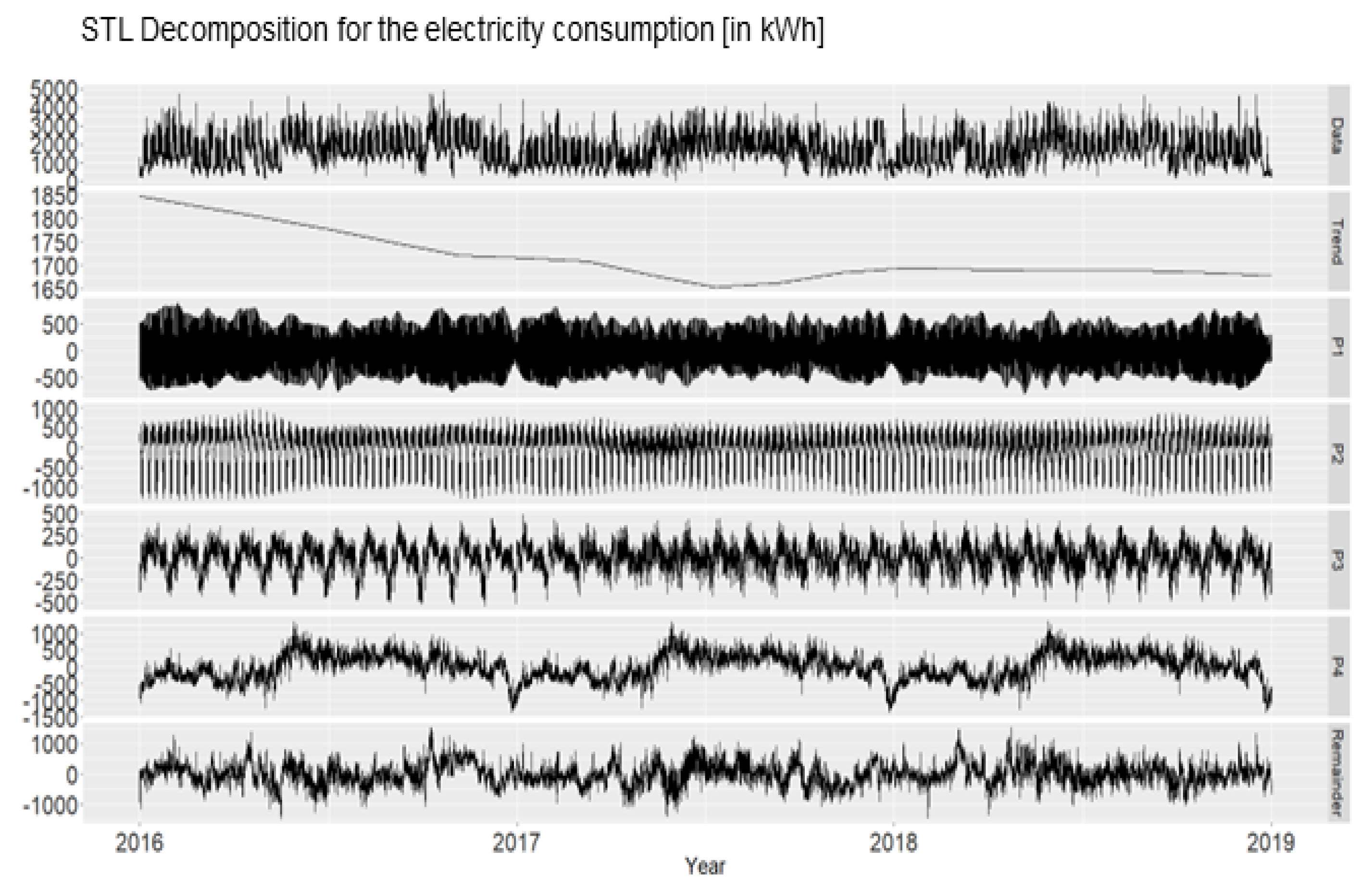
2.2. Time Series Decomposition

Time series can exhibit a variety of patterns, and it is often helpful to split said time series into several components, each representing an underlying pattern category. There are two forms of classical decompositions, additive and multiplicative decompositions. The first method is used when the magnitude of the seasonal fluctuations, or the variation around the trend-cycle, does not depend on the level of the time series, while the latter is applied if the seasonal effect tends to increase as the trend increases. We say that the data are seasonally adjusted, if all underlying seasonal components have been removed from the original data. In the case of an additive model, the seasonal time series $Y_t$ can be decomposed into a seasonal component $S_t$ and non-seasonal components such as a trend-cycle $T_t$ and irregular components $R_t$. It is given by:

$$Y_t=S_t+T_t+R_t$$

(4)

Decomposing a time series into different components has been a main research area for a long time. It started with Persons [22], in the early 1920s, by decomposing the time series into its most important components. Since then many different decomposition methods along with seasonal adjustment were suggested. The most important one is the X-11 method developed by the Bureau of the Census in 1950s and 1960s [23]. It has been expanded recently into the X-13ARIMA-SEATS program [24].

The STL method is a versatile and robust way of decomposing time series and was developed by [21]. STL is an acronym for “Seasonal and Trend decomposition using Loess”. The STL procedure is carried out in an iterated cycle of detrending and then updating the seasonal component from the resulting sub-series. At every iteration, the robustness weights are formed based on the estimated irregular component; the former are then used to down-weight outlying observations in subsequent calculations. The iterated cycle is therefore composed of two recursive procedures, the inner and outer loops [25].

Assume our data are represented by Equation (4); the basic steps involved in STL to produce seasonally adjusted data and trend estimation are given in the original paper of Cleveland [21]. Suppose that the number of each seasonal periods is given by $n_{\left(p\right)}$. In the inner loop, each pass $n_{\left(i\right)}$ applies seasonal smoothing that updates the seasonal component, followed by trend smoothing that updates the trend component. Let $S_t^{\left(k\right)}$ and $T_t^{\left(k\right)}$ be the seasonal and trend components at the end of the kth pass, then updating those components into the pass $k+1$ is usually conducted using the following steps:

1.

A detrended series $Y_t-T_t$ is computed;

2.

In the second step, the cycle-subseries are formed and smoothed on the detrended series using Loess with $h=n_{\left(s\right)}$ and $d=1$. For example, for a monthly series with a yearly seasonality $n_{\left(p\right)}=12$, the first subseries consists of the January values, the second is the February values, and so on. The collection of smoothed values for the entire cycle-subseries is a temporary seasonal series, $C_t^{(k+1)}$;

3.

A low-pass filter is applied into the smoothed cycle-subseries $C_t^{(k+1)}$ and consists of the three moving averages followed one by one, where the two first moving averages have a length of $n_{\left(p\right)}$, while the last has a length of 3. In the end, a Loess smoothing with $d=1$ and $h=n_{\left(l\right)}$ is applied, and the output is defined as $L_t^{(k+1)}$;

4.

The seasonal component from the $(k+1)$st loop is $S_t^{(k+1)}=C_t^{(k+1)}-L_t^{(k+1)}$;

5.

A deseasonalized series $Y_t-S_t^{(k+1)}$ is computed;

6.

In the last step, the trend component is estimated using the deseasonalized series and smoothing them with $h=n_{\left(t\right)}$ and $d=1$ and is given by $T_t^{(k+1)}$.

Each pass of the outer loop $n_{\left(o\right)}$ consists of the inner loop followed by a computation of robustness weights and starts first by removing both the estimated seasonal and trend components received from the inner loop. Then, the remainder is:

$$R_t=Y_t-S_t-T_t$$

For each time point $Y_t$, a weight is defined. These robustness weights reflect how extreme $R_t$ is. For example, an outlier in the data that results in a very large $|R_t|$ will have a small or zero weight. Therefore, introduce:

$$v=6median\left(\right|R_t\left|\right)$$

Then, the robustness weight at time point t is:

$$r_t=B\left(\frac{|R_t|}{v}\right)$$

where B is the bisquare weight function:

$$B\left(\alpha \right)=\{\begin{array}{cc}\hfill {(1-{\alpha }^2)}^2\hfill & \mathrm{for} 0\le \alpha <1\\ \hfill 0\hfill & \mathrm{for} \alpha >1\end{array}$$

The inner loop now is repeated, but in the smoothness of steps 2 and 6, the neighborhood weight for a value at time t is multiplied by the robustness weight $r_t$. Hence, the STL method has 6 parameters $n_{\left(p\right)}$, $n_{\left(i\right)}$, $n_{\left(o\right)}$, $n_{\left(l\right)}$, $n_{\left(t\right)}$, $n_{\left(s\right)}$ that in practice are mostly chosen in an automated way.

We have chosen the STL decomposition procedure as opposed to other decomposition methods in the literature for the following reasons:

• Unlike SEATS and X11, STL can handle any type of seasonality, not only monthly and quarterly data;
• The seasonal component is allowed to change over time, and the rate of change can be controlled by the user;
• The smoothness of the trend-cycle can also be controlled by the user;
• It can be robust to outliers (i.e., the user can specify a robust decomposition), so that occasional unusual observations will not affect the estimates of the trend-cycle and seasonal components. They will, however, affect the remainder component;
• The implementation of the STL procedure is based purely on numerical methods and does not require any mathematical modelling.

On the other hand, the STL method also carries some disadvantages. In particular, it does not handle the working day or calendar variation automatically, and it only provides facilities for additive decompositions [26]. However, it is also possible to handle a multiplicative decomposition by first taking the logarithm of the data, which would obviously emulate an additive decomposition. Following this, the transformation of the acquired components would then need to be reversed. Decompositions that lie somewhere in-between the additive and multiplicative can be obtained via a Box-Cox transformation $(Y_t^{\lambda }-1)/\lambda$ of the respective data with $0<\lambda <1$.

2.3. Seasonal ARIMA Models

Seasonal ARIMA models ($\mathit{SARIMA}(p,d,q){(P,D,Q)}_s$) are linear time series of past observations and random errors and can be defined as:

$${\Phi }_P\left(B^s\right){\varphi }_p\left(B\right){(1-B^s)}^D{(1-B)}^d{y}_t={\Theta }_Q\left(B^s\right){\theta }_q\left(B\right){ϵ}_t$$

(5)

where s is the seasonal length, ${(1-B)}^d$ and ${(1-B^s)}^D$ are the nonseasonal and seasonal differencing operators, while ${\Phi }_P,{\varphi }_p,{\Theta }_Q,\mathrm{and}{\theta }_q$ are polynomials of orders $P,p,Q,\mathrm{and}q$, respectively. B is the back shift operator expressed by $B{y}_t=y_{t-1}$ and ${ϵ}_t$ is a sequence of white noises with zero mean and constant variance.

A multi-step model-building strategy for seasonal ARIMA models was introduced in [27]. It consists of model specification, model fitting, and model diagnostics. In model specification, the autocorrelation function (ACF) and partial autocorrelation function (PACF) of the sample data are used to identify the orders of the ARIMA model. At this stage, data transformation such as a Box-Cox transformation can be used to make a time series stationary. A stationary series is one whose properties do not depend on the time at which the series is observed. Model fitting consists of finding the best estimate of the parameters within a given model. Methods such as maximum likelihood estimation (MLE) and information criteria such as $AI{C}_c$ are mainly used to determine the unknown parameters of the model. Model diagnostics analyze the quality of the model chosen. This phase consists of different diagnostic statistics and plots of the residuals that are used to defined the most parsimonious model that is chosen for forecasting.

2.4. Dynamic Regression Models

Standard regression models cannot represent the delicate interdependencies of time series dynamics that can be handled by seasonal $\mathit{ARIMA}$ models. In this section, the error term of the regression model will therefore contain auto-correlation. Suppose that we have the observations $\{y_1,\dots ,y_n\}$ which are given as a linear function of the k predictor variables $\{x_{1,t},\dots ,x_{k,t}\}$ and the error series ${\eta }_t$, which follows an $\mathit{ARIMA}$ model. Then, the dynamic regression model with $\mathit{ARIMA}(p,d,q)$ errors is defined as:

$$\begin{array}{c}\hfill y_t={\beta }_0+{\beta }_1{x}_{1,t}+\dots +{\beta }_k{x}_{k,t}+{\eta }_t\hfill \\ \hfill {\varphi }_p\left(B\right){(1-B)}^d{\eta }_t={\theta }_q\left(B\right){ϵ}_t\hfill \end{array}$$

(6)

where ${ϵ}_t$ is a white noise series. To estimate the parameters of the model, we minimize the sum of squared ${ϵ}_t$ values. This avoids problems with the $AI{C}_c$ values in this setting [26].

2.5. Average Method

An average method is a simple forecasting method, where the forecasts of all future values are given as the average (or “mean”) of the observed values of corresponding past observations (“historical data”) [26]. As a simple example, suppose that we are at time t and consider the last three observations as the corresponding history, then the average method predicts $y_{t+1}$ as:

$${\widehat{Y}}_{t+1}=\overline{\mathrm{Y}}=\frac{Y_t+Y_{t-1}+Y_{t-2}}{3}$$

3. Predicting Electricity Consumption: Conceptual Issues

Our research aims to provide a conventional benchmark prediction model for electricity consumption. By conventional, we mean a non-neural network based approach, specifically. Furthermore, we would like to come up with a prediction method that at least beats the average-based method used by the electricity provider we collaborated with. The major research questions we investigate are:

• Are dynamic regression models capable of modelling electricity consumption data and generating acceptable forecasts?
• When is it hard to beat the average-method-variant?
• When does at least the best method perform well?
• When does no method perform well?

We will use the eight real data sets to answer these and other related questions.

On top of it, our task was to come up with a “conventional” benchmark prediction model (no neural networks were allowed) that beats the averaging method. The exact prediction should be all 15 min consumption amounts of the individual customer for the next day. Even more, we were not allowed to use the data of today, as in the practical application, they are not known before tomorrow. Thus, we had to predict 96 values ahead in one shot which—in our minds—is quite an ambitious task.

Below, we will describe the data, the methods that we compare for predicting electricity consumption, their actual use and the type of error measures for judging the forecasting performance of the different methods.

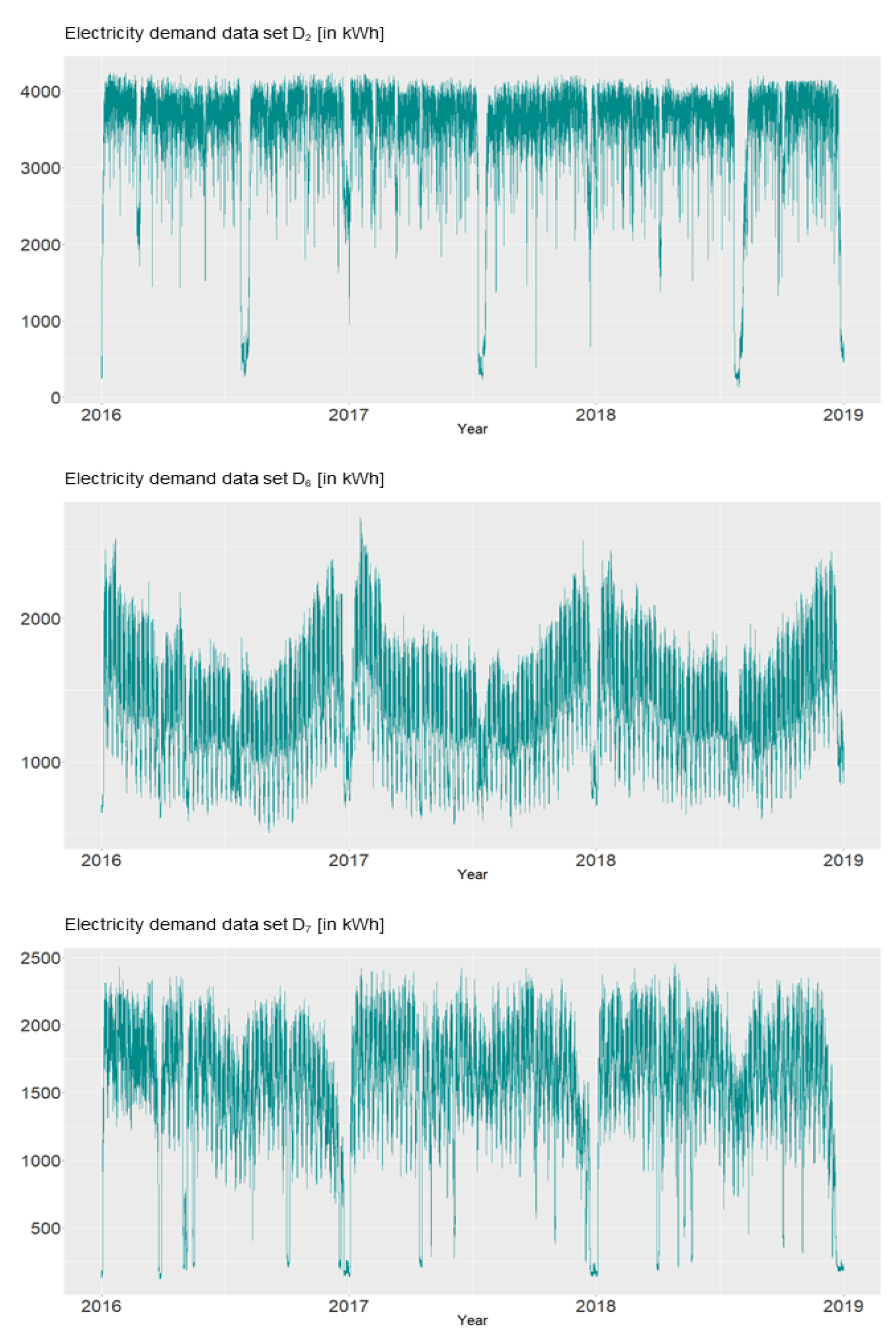
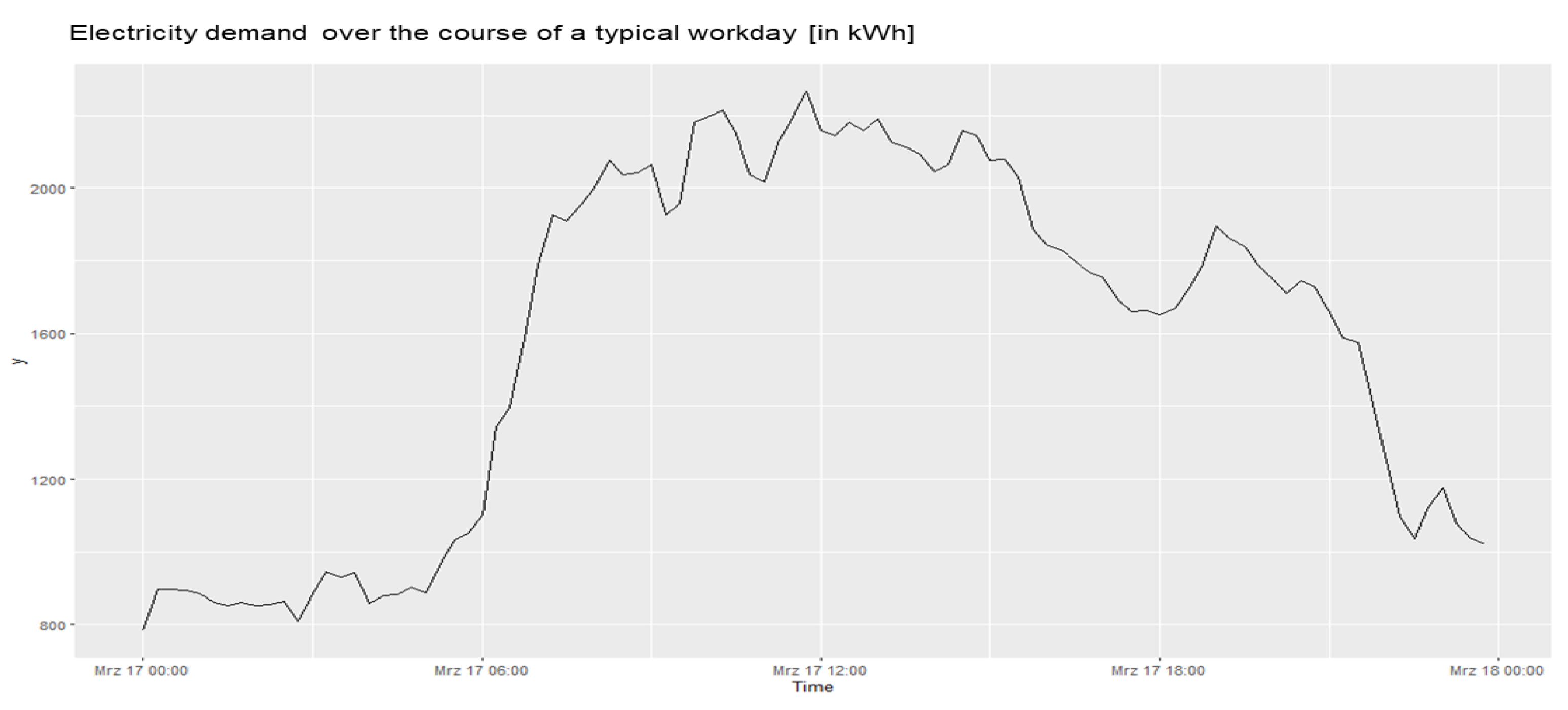
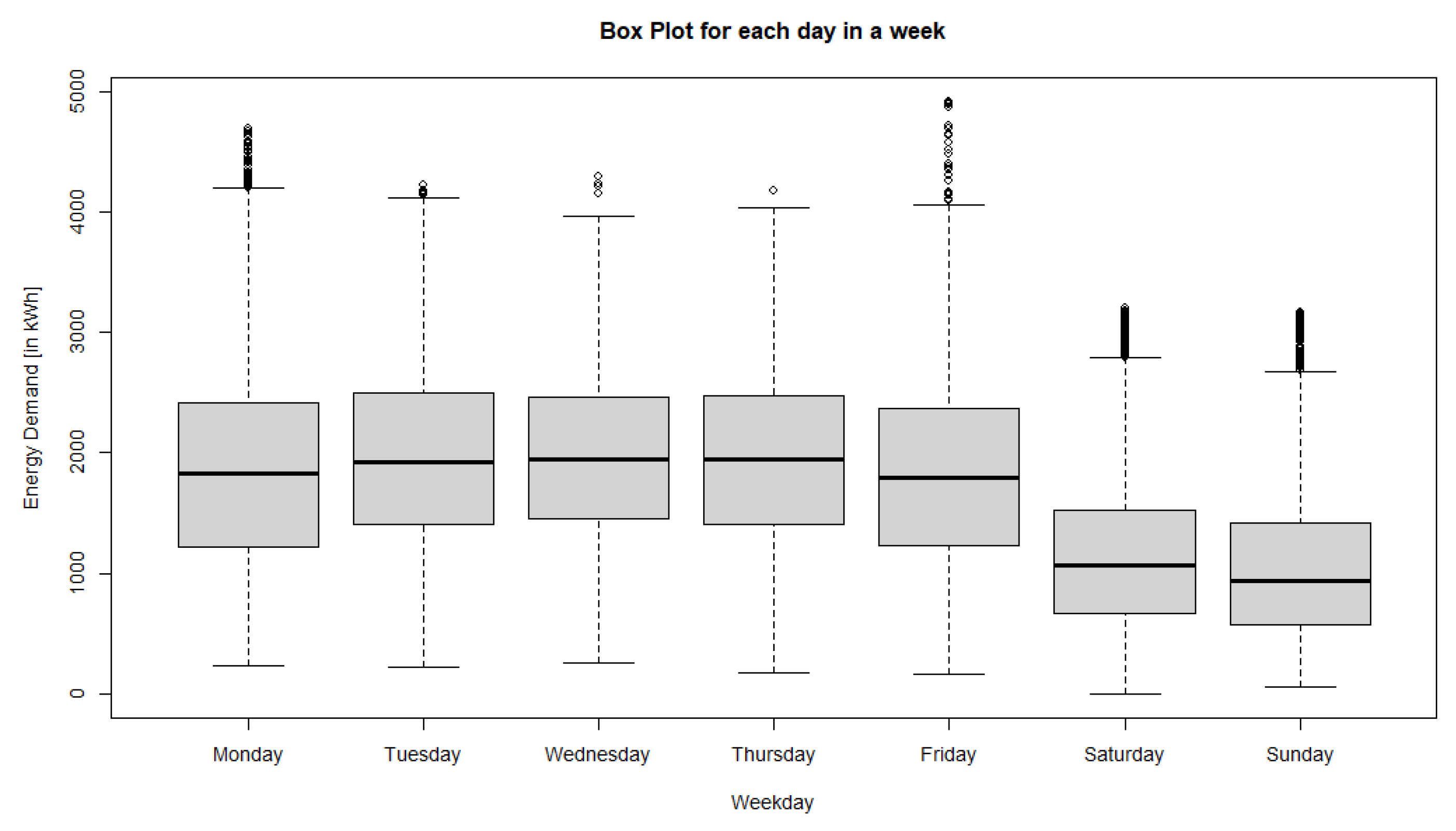
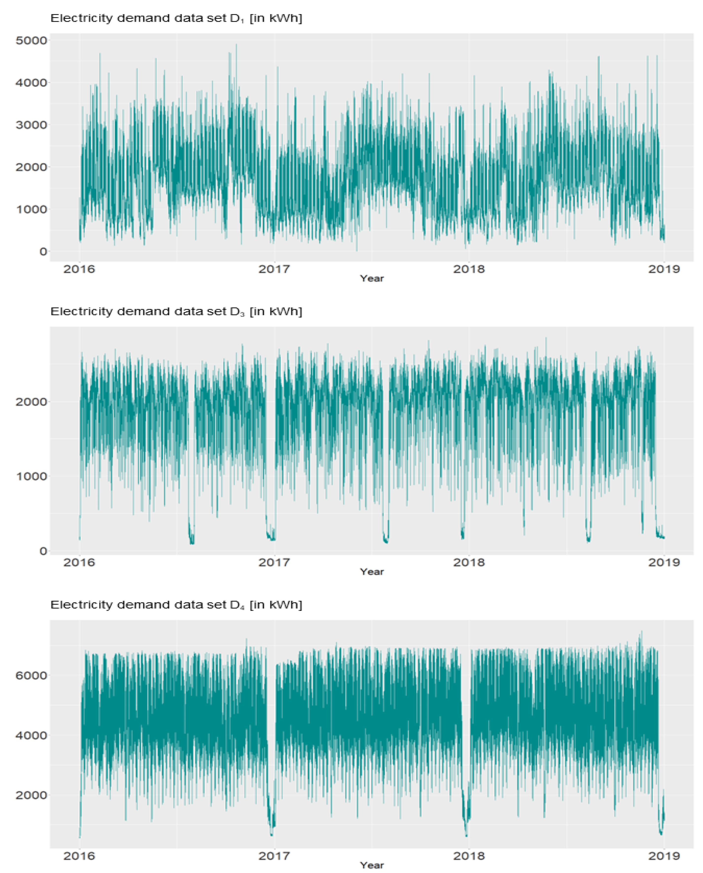
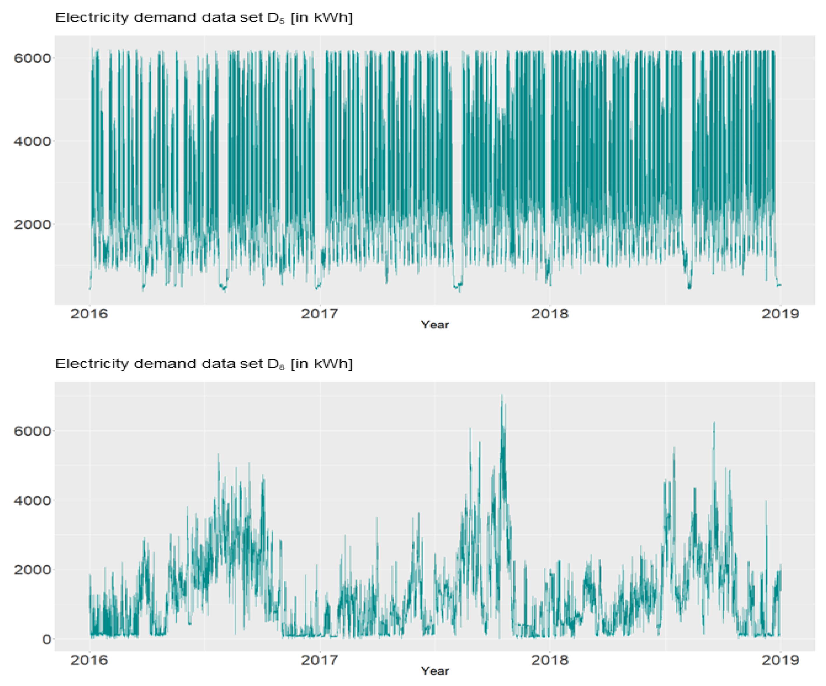
3.1. Data Exploration and Analysis

As mentioned before, the energy demand data are provided by a local electricity supplier, and, for the sake of simplicity and confidentiality, we will use an anonymous way of abbreviation for the eight data sets displayed in Figure 1 and Figure A1 (see Appendix A for further time series data of electricity consumption), e.g., “$D_1$”, “$D_2$”, “$D_3$”, “$D_4$”, “$D_5$”, “$D_6$”, “$D_7$”, and “$D_8$”. These represent high frequency data sets (96 data points per day represented in kWh) with potentially multiple seasonalities and a weak trend component that usually contain three years worth of observations starting from 2016. In general, the customers’ consumption behaviors are quite heterogeneous. For example, the top diagram in Figure 1 shows the demand for data “$D_2$” which significantly decreases at the beginning of every quarter. In the last diagram of Figure 1, the consumption of “$D_7$” displays sharp decreases during the given years. The electricity demand for data “$D_6$” decreases smoothly in the middle of the years, which means that the consumption is high in January and decreases until approximately the ninth month with an increase thereafter.

Moreover, the figures below provide some context regarding the general structure as well as the characteric behavior of energy consumption. Specifically, Figure 2 displays a very typical behavior of electricity consumption at a workplace over the course of a workday. It is fairly intuitive that the consumption is at its lowest at the beginning of the day and does not significantly increase until work has started early in the morning. The peak is usually reached in the early afternoon and then starts steadily decreasing until the workday is over. On the other hand, Figure 3 contains a boxplot that highlights some differences between workdays and weekend days. It is evident that the consumption level is significantly lower during the weekend, as the workload in that time period is usually far lower as well.

Remark 1

(Predictable anomalies). Some data points appear to be anomalies, as they represent a very notable downward spike. Some of those instances are actually predictable in the sense that the customer has announced a maintenance action on that time leading to a reduced electricity consumption. Since this is not a regular event, it is hard to learn such a pattern. Even more, it will have an impact on learning the regular variations. It would therefore be suitable to eliminate these data points. However, since we did not have the full information on these anomalies, we could not simply exclude them.

3.2. Research Design

In order to forecast the electricity demand, we consider two dynamic regression approaches.

3.2.1. Dynamic Harmonic Regression

Here, we use the Fourier series approach to model the seasonal periodicities. Furthermore, temperature values taken from the provider Deutscher Wetterdienst [28] and working days occurring in the same region of the local electricity supplier will be used as predictor variables.

This model is represented by the following formula:

$$\begin{array}{c}\hfill y_t={\beta }_0+{\beta }_{1}t+{\beta }_2{x}_{2,t}+{\beta }_3{x}_{3,t}+\sum _{i=1}^M\sum _{k=1}^{K_i}({\beta }_{4,k}cos\frac{2\pi tk}{p_i}+{\beta }_{5,k}sin\frac{2\pi tk}{p_i})+{\eta }_t\hfill \\ \hfill {\varphi }_p\left(B\right){(1-B)}^d{\eta }_t={\theta }_q\left(B\right){ϵ}_t\hfill \end{array}$$

(7)

where $x_{2,t},x_{3,t}$ are predictor variables as working days and temperature values. ‘M’ corresponds to the number of seasonal periods. In our case, for 15 min data sets, we have considered four seasonal periods: daily, weekly, monthly and yearly seasonality. For each of the periods ‘$p_i$’, the number of Fourier terms $\left(K_i\right)$ are chosen to find the best statistical model for a given set of data. In order to determine the adequate number of Fourier terms corresponding to each of the periods, the AIC values of the ARIMA model with varying Fourier terms were calculated. In order to keep a reasonable computation time, we have restricted each $K_i$ to be within $\{1,\dots ,10\}$. As a result, for all data sets, $K=(10,8,8,8)$ were found to be the best choice.

3.2.2. Dynamic Regression Model with STL Decomposition

The trend and seasonalities are estimated first using the STL method and then those are included as independent variables in the regression model, as follows:

$$\begin{array}{c}\hfill log\left(y_t\right)={\beta }_0+{\beta }_{1}ST{L}_t+{\beta }_{2}ST{L}_{p_1}+{\beta }_{3}ST{L}_{p_2}+{\beta }_{4}ST{L}_{p_3}\hfill \\ \hfill +{\beta }_{5}ST{L}_{p_4}+{\eta }_t\hfill \\ \hfill {\varphi }_p\left(B\right){(1-B)}^d{\eta }_t={\theta }_q\left(B\right){ϵ}_t\hfill \end{array}$$

(8)

$ST{L}_t$ specifies the estimated trend values from the STL method, while $ST{L}_{p_1}$, $ST{L}_{p_2}$, $ST{L}_{p_3}$, $ST{L}_{p_4}$ are the predictor variables for the seasonal periodicities taken from the method STL with periods $p_1=96,p_2=672,p_3=2922,p_4$ = 35,063, for the daily, weekly, monthly and yearly seasonality, respectively. The estimated trend and seasonal periods were obtained using R as a programming language (the hyperparameters for the ARIMA method were found by using the auto.arima function in R. To obtain the STL parameters, the seasonal package in R was used). For instance, Figure 4 shows an example of the multiple STL method applied to the data $D_1$ and gives an estimation of these components, and, moreover, the trend and the remainder component. To properly interpret this graph, it is important to notice the vertical scales. In this case, the trend and the monthly seasonality have relatively narrow ranges compared to the other components: the trend decreases until the middle of 2017 and then stays the same level for the remaining part. The monthly seasonality is weak. Moreover, a log transformation is performed on all data sets. Estimation of the Box-Cox lambda leads to a value larger than zero which suggests one to use log-transformed data for the STL-method. However, the STL method expects an additive decomposition, which is why it is reasonable to apply the logarithm first.

To choose the appropriate model, we separate the available data into training and test data. Three forecasting horizons, two-days, seven-days, and a month ahead, are performed on the 15 min electricity demand data using the two approaches mentioned above. For the dynamic regression model with the STL decomposition method, the trend and seasonal values necessary for the test set were obtained using two techniques. Firstly, the trend values were forecasted using a linear regression, while the seasonal values were simply taken from the last year of the estimated component, and secondly, the trend and seasonal values were forecasted using the STL method. Among the two techniques, we choose the best one to report its testing results.

4. Numerical Results

4.1. Dynamic Harmonic Regression

Figure 5, Figure 6, Figure 7 and Figure 8 (see Appendix A, Figure A2, Figure A3 and Figure A4 for other data sets) show the actual consumption compared to the forecasted one obtained from the Dynamic Harmonic Regression model, as well as the average method applied from the local electricity supplier for all the data sets, for one month, seven days, and two days ahead of the forecasting horizon, respectively. For example, the best time series forecasting model fitting from the dynamic harmonic regression with temperature, working days, and the chosen Fourier terms as independent variables and an $ARIMA(2,1,1)$ model for the error term for the data $“D_1”$ is given by:

$$\begin{array}{c}\hfill y_t=1525-0.0015trend-4.598temp+426.3working+\hfill \\ \hfill \sum _{i=1}^M\sum _{k=1}^{K_i}({\beta }_{4,k}cos\frac{2\pi tk}{p_i}+{\beta }_{5,k}sin\frac{2\pi tk}{p_i})+{\eta }_t\hfill \\ \hfill {\varphi }_2\left(B\right)(1-B){\eta }_t={\theta }_1\left(B\right){ϵ}_t\hfill \end{array}$$

with $p_1=96,p_2=672,p_3=2922,p_4=\mathrm{35,063}$, and $K=(10,8,8,8)$ and:

$$\begin{array}{c}\hfill {\varphi }_2\left(B\right)=1-0.7273B+0.1427B^2\hfill \\ \hfill {\theta }_1\left(B\right)=1+0.6125B\hfill \end{array}$$

The forecast results obtained from the Dynamic Harmonic Regression are different depending on the forecasting horizon, as the input sets slightly differ (note that the method gets more information for the shorter time period predictions), while the currently employed average approach remains the same over the different periods. For example, the predictions from the two models for the three forecasting horizons of data set “$D_2$” (see e.g., Figure 5) do not capture the stark drop in demand, which is a result of the holidays at the end of the year. However, a different performance of the forecasts is obtained for the data “$D_6$”. All three monthly, weekly, and the two daily forecasts are predicted very well from the dynamic harmonic regression model and the average method with small differences to the actually observed values (see, e.g., Figure 6).

Whereas the average forecasts of the data “$D_4$” in Figure 7 yield a higher accuracy than the dynamic harmonic regression, especially capturing the lower values on the last days of the month, we observe a different performance for the data “$D_3$” in Figure 8. Here, the dynamic harmonic regression model outperforms the average approach for each of the forecast horizons, especially for the very short forecasting period. In the Appendix A (Figure A2, Figure A3 and Figure A4) you will find the forecasting results for the other data sets with analogue results.

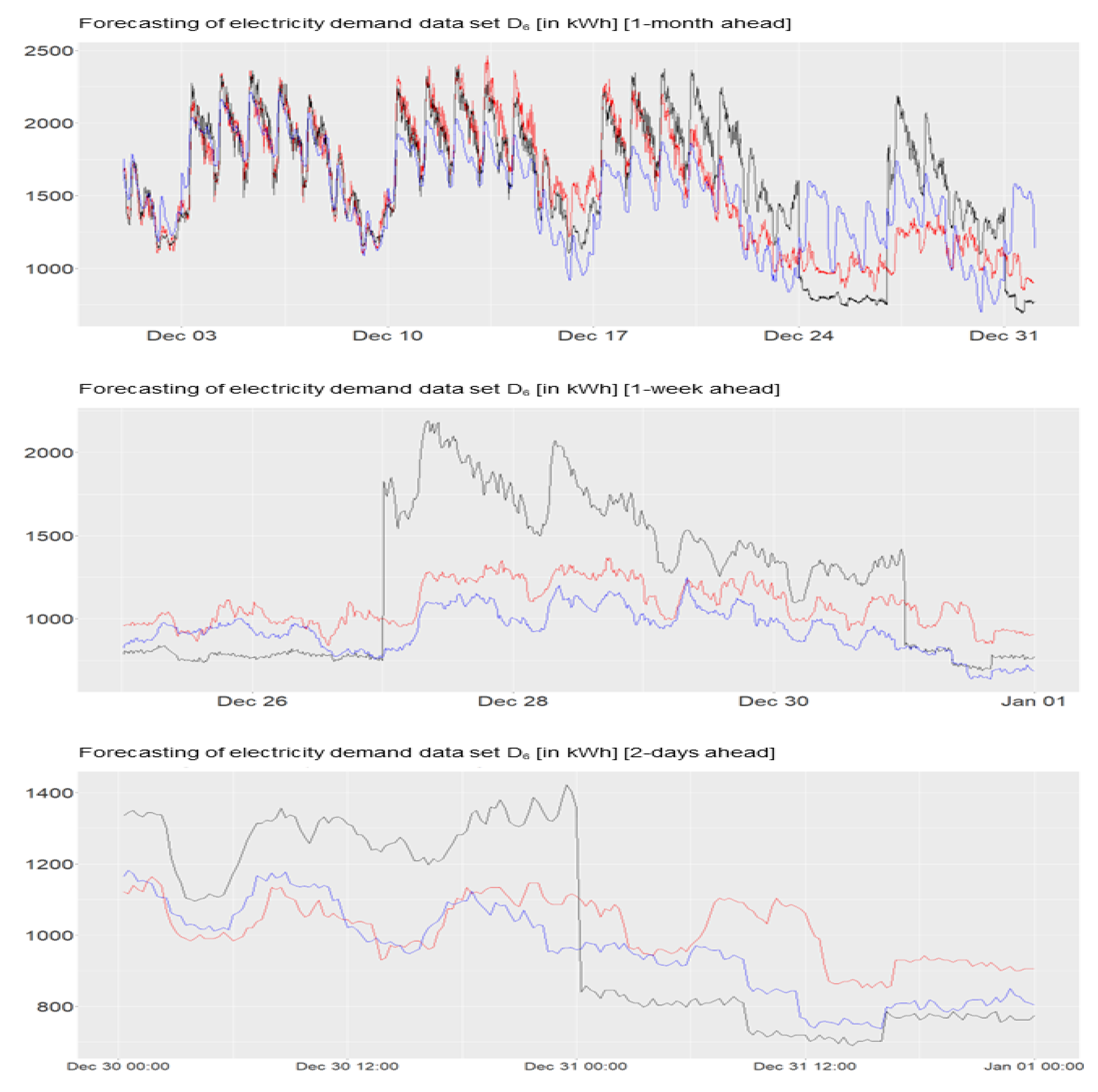
4.2. Dynamic Regression with STL

The fitted version of the Dynamic Regression with STL for data “$D_4$” is given by:

$$\begin{array}{c}\hfill log\left(y_t\right)=-1.297+1.008ST{L}_t+1.077ST{L}_{p_1}+1.028ST{L}_{p_2}+1.124ST{L}_{p_3}+1.01ST{L}_{p_4}+{\eta }_t\hfill \\ \hfill {\varphi }_1\left(B\right){\eta }_t={\theta }_3\left(B\right){ϵ}_t\hfill \end{array}$$

with $p_1=96,p_2=672,p_3=2922,p_4=\mathrm{35,063}$, and

$$\begin{array}{c}\hfill {\varphi }_1\left(B\right)=1-0.9839B\hfill \\ \hfill {\theta }_3\left(B\right)=1+0.2253B+0.2700B^2+0.2399B^3\hfill \end{array}$$

Test on Individual Regression Coefficients (t Test)

Performing the t-test for the individual coefficients on the regression part, we found that the temperature and working days did not prove to be significant for the model and therefore they were removed. The statistics for the model corresponding to the remaining variables are given below. We have obtained similar results when performing the analysis for the remaining data sets.

•     Residuals:  Min             1Q          Median      3Q           Max
•                    −2649.28      −341.56         3.91        347.19      2328.30
• Coefficients:
•                                         Estimate   Std.   Error   t value   Pr(>|t|)
• (Intercept)                   −1.297428       7.999 × 10    −5.071   3.96 × 10⁻⁰⁷   ***
• STL_t                            1.088 × 10    1.747 × 10⁻⁰²   62.286   <   2 × 10⁻¹⁶   ***
• STL_p1                         1.077 × 10    5.120 × 10⁻⁰³   210.315   <   2 × 10⁻¹⁶   ***
• STL_p2                         1.028 × 10    2.901 × 10⁻⁰³   354.392   <   2 × 10⁻¹⁶   ***
• STL_p3                         1.124 × 10    6.259 × 10⁻⁰³   179.633   <   2 × 10⁻¹⁶   ***
• STL_p4                         1.010 × 10    2.268 × 10⁻⁰³   445.197   <   2 × 10⁻¹⁶   ***
• ---
• Signif.   codes:    0   ***   0.001   **   0.01   *   0.05   .   0.1     1
• Residual   standard   error:   516.5   on   102233   degrees   of   freedom
• Multiple   R-squared:    0.8041,          Adjusted   R-squared:      0.8041
• F-statistic:   8.393 × 10⁴   on   5   and   102233 DF,    p-value:   <   2.2 × 10⁻¹⁶

The forecasted values of the STL method outperform the average method on all the data sets. For example, for the data “$D_3$” (see Figure 9), the dynamic regression with STL has captured the trend and seasonal components in the data quite well without the need for further independent variables, as included in the first proposed model. Even though the forecasts for the monthly, weekly, and daily values obtained from the STL method are better than those of the average method, there is some unusual behavior that the dynamic regression with STL did not manage to capture. This can be observed for the monthly and weekly forecasting results for the data “$D_2$” (see Figure 10).

Furthermore, for regular data sets such as the values of “$D_6$” (see Figure 11), both models achieved good results capturing the dynamics in the series with some small differences in favour of the STL method. In general, good forecasting results of the STL method can be observed as well for the other data sets in the Appendix A (Figure A5, Figure A6, and Figure A7).

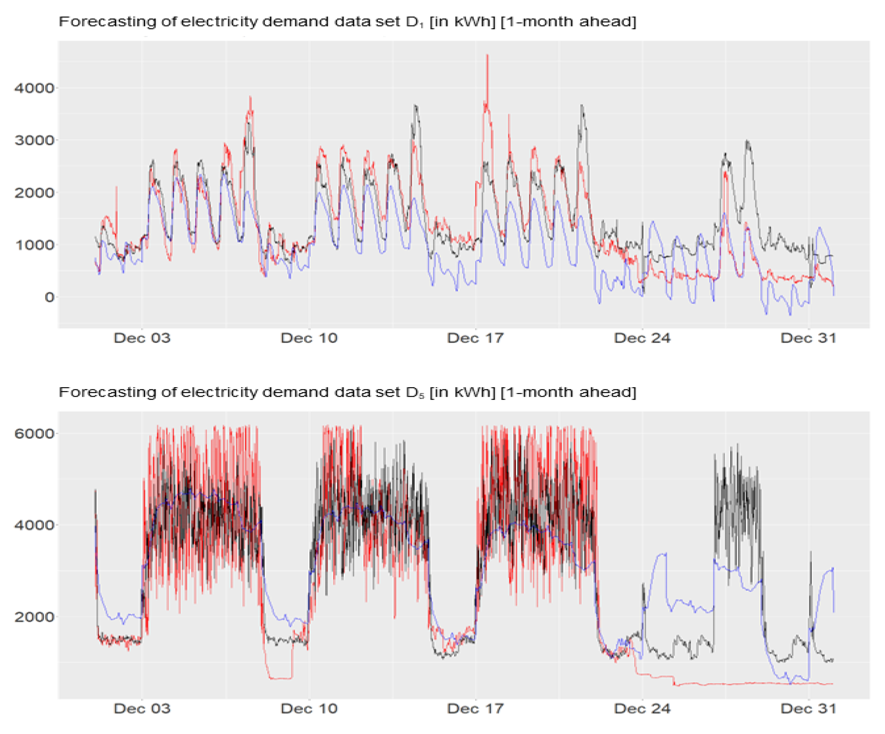
4.3. Comparison of the Model Performances

The purpose of our research was to find a conventional benchmark prediction method for electricity consumption. To this end, we have developed two dynamic regression forecasting models and compared them with the average method used by the electricity provider. As stated in the introduction, we have considered the RMSE, MAPE and MAE in order to measure and compare the forecasting results across the one-month, seven-day, and two-day forecasting horizons.

With regard to the research questions posed in Section 3, the results shown in

Table 1. Comparison of the forecasting methods for a forecasting horizon of one month.

Data	Model	RMSE	MAPE	MAE
“$D_1$”	Average Method	526.37	52.99	395.51
	Dynamic Harmonic Regression	658.13	50.65	536.50
	Dynamic Regression with STL	502.12	40.52	365.18
“$D_2$”	Average Method	1301.08	89.18	811.46
	Dynamic Harmonic Regression	1099.71	78.34	725.62
	Dynamic Regression with STL	953.37	62.12	721.95
“$D_3$”	Average Method	1138.69	366.40	908.28
	Dynamic Harmonic Regression	813.07	280.83	753.46
	Dynamic Regression with STL	403.32	74.34	302.41
“$D_4$”	Average Method	891.80	35.19	675.77
	Dynamic Harmonic Regression	1455.22	70.84	1263.73
	Dynamic Regression with STL	1095.55	23.65	769.45
“$D_5$”	Average Method	1374.82	93.59	966.60
	Dynamic Harmonic Regression	1290.3	98.48	1017.46
	Dynamic Regression with STL	1250	48.33	865.28
“$D_6$”	Average Method	244.05	13.55	176.53
	Dynamic Harmonic Regression	253.86	14.49	203.80
	Dynamic Regression with STL	200.88	12.03	161.64
“$D_7$”	Average Method	672.27	173.25	548.95
	Dynamic Harmonic Regression	402.88	96.73	324.12
	Dynamic Regression with STL	354.39	48.57	270.09
“$D_8$”	Average Method	746.45	Inf	561.90
	Dynamic Harmonic Regression	838.06	Inf	705.59
	Dynamic Regression with STL	723.57	Inf	580.34

,

Table 2. Comparison of the forecasting methods for a forecasting horizon of seven days.

Data	Model	RMSE	MAPE	MAE
“$D_1$”	Average Method	810.40	154.53	715.87
	Dynamic Harmonic Regression	467.06	86.48	370.42
	Dynamic Regression with STL	365.18	49.90	256.27
“$D_2$”	Average Method	2592.55	357.94	2512.66
	Dynamic Harmonic Regression	2130.54	303.97	1914.59
	Dynamic Regression with STL	2044.07	280.74	1913.46
“$D_3$”	Average Method	1396.29	694.94	1266.59
	Dynamic Harmonic Regression	884.68	478.95	867.47
	Dynamic Regression with STL	116.17	58.51	104.95
“$D_4$”	Average Method	527.80	53.55	450.46
	Dynamic Harmonic Regression	1136.01	103.28	1000.73
	Dynamic Regression with STL	225.77	13.86	163.78
“$D_5$”	Average Method	2179.19	310.30	1645.88
	Dynamic Harmonic Regression	1742.89	283.96	1507.42
	Dynamic Regression with STL	158.46	22.99	124.11
“$D_6$”	Average Method	379.64	28.96	323.32
	Dynamic Harmonic Regression	277.45	21.48	228.75
	Dynamic Regression with STL	171.56	13.97	152.21
“$D_7$”	Average Method	647.05	287.58	591.61
	Dynamic Harmonic Regression	486.13	183.64	385.78
	Dynamic Regression with STL	41.55	16.80	34.62
“$D_8$”	Average Method	869.15	201.53	713.78
	Dynamic Harmonic Regression	828.33	340.48	731.67
	Dynamic Regression with STL	700.69	76.51	452.43

and

Table 3. Comparison of the forecasting methods for a forecasting horizon of two days.

Data	Model	RMSE	MAPE	MAE
“$D_1$”	Average Method	475.24	132.80	448.74
	Dynamic Harmonic Regression	686.95	141.99	510.26
	Dynamic Regression with STL	149.91	36.69	126.49
“$D_2$”	Average Method	2678.93	478.91	2622.51
	Dynamic Harmonic Regression	1475.34	253.16	1364.24
	Dynamic Regression with STL	537.83	88.02	481.78
“$D_3$”	Average Method	1365.10	699.81	1241.89
	Dynamic Harmonic Regression	104.87	50.17	89.20
	Dynamic Regression with STL	91.96	46.28	81.54
“$D_4$”	Average Method	230.65	16.49	213.28
	Dynamic Harmonic Regression	1149.15	80.77	1028.17
	Dynamic Regression with STL	247.50	15.38	200.62
“$D_5$”	Average Method	873.30	149.50	796.78
	Dynamic Harmonic Regression	1339.25	177.18	938.68
	Dynamic Regression with STL	114.59	17.67	93.82
“$D_6$”	Average Method	220.30	20.57	210.58
	Dynamic Harmonic Regression	366.04	31.05	303.20
	Dynamic Regression with STL	107.33	8.47	85.51
“$D_7$”	Average Method	395.63	168.81	339.67
	Dynamic Harmonic Regression	428.61	173.86	349.50
	Dynamic Regression with STL	49.28	23.71	47.93
“$D_8$”	Average Method	727.85	37.68	665.43
	Dynamic Harmonic Regression	1780.46	91.34	1721.95
	Dynamic Regression with STL	669.09	37.08	645.56

below demonstrate that dynamic regression models are capable of capturing the complexity of the electricity demand, especially combined with the seasonal and trend adjustment approach using the STL method. However, it was hard to beat the average method when the data contained outliers caused by planned maintenance by the customer, information that has been provided to the electricity provider in advance (see also Remark 1). Notably, this was the case with data set “$D_4$” (see Figure 7). In fact, this is the only instance where the forecasting of the electrity provider outperformed the dynamic regression with STL.

On the other hand, the dynamic regression method with STL outperforms the other methods in terms of RMSE, MAPE and MAE for every single data set. The estimation of the seasonality and the trend by the STL method was proved to capture the relevant information in the data, especially for shorter periods as well as holiday periods. This is evident even from just taking a look at the Figure A5, Figure A6, and Figure A7. The results computed from the dynamic harmonic regression, where the Fourier series approach is used to estimate the seasonal periodicities in our data, mainly provide good performance measures when the seasonality patterns do not change over time. As they are assumed to be fixed in the Fourier series approach, the estimates become worse when the dynamic regression with STL proves to be quite accurate in its forecasting.

The dynamic regression models fail to predict in some periods when there are some unusual jumps such as reductions of workloads occurring in the data and where usually the average method of the electricity provider works well. Of course, the latter is modified by using this additional information provided by the customer in advance, information that the dynamic regression methods did not have. Thus, one should not consider this as a better performance of the average method. Further, this simple average method does not always capture the trend in the data, especially when there are sudden changes in the consumption (that have not been announced to the provider) that do not occur regularly over time. Hence, the forecasts provided from this method do not really approximate the real consumption.

In general, for the time series demonstrating a close to regular behaviour in time, the forecasting performances of the three methods are quite close. Examples of data sets where this is the case are: “$D_1$”, “$D_6$”, or “$D_8$”. A completely different situation can be observed in the case of the data set “$D_7$”, where the dynamic regression with STL proves superior to the dynamic harmonic regression across all three forecasting horizons, which clearly beats the average method on its own.

Interestingly enough, the proposed methods perform differently depending on the forecasting horizon. The dynamic regression with STL intuitively improves for shorter forecasting horizons. Contrary to that, the dynamic harmonic regression exhibits the exact opposite behavior and improves for longer forecasting horizons.

For the sake of completion, we provide the forecasting results of the consumption for two days ahead where the test set now is November 2018 (see

Table A1. Comparison between dynamic regression with STL and the average method for a forecasting horizon of two days in November.

Data	Model	RMSE	MAPE	MAE
“$D_1$”	Average Method	759.20	25.74	535.56
	Dynamic Regression with STL	712.53	20.19	465.83
“$D_2$”	Average Method	394.81	8.52	314.64
	Dynamic Regression with STL	296.42	6.33	236.57
“$D_3$”	Average Method	295.23	11.92	223.94
	Dynamic Regression with STL	283.24	12.15	246.71
“$D_4$”	Average Method	869.86	13.53	724.98
	Dynamic Regression with STL	803.29	12.23	649.67
“$D_5$”	Average Method	1312.93	27.15	1100.95
	Dynamic Regression with STL	1276.12	26.48	1081.26
“$D_6$”	Average Method	145.23	5.93	105.05
	Dynamic Regression with STL	131.7767	5.86	107.68
“$D_7$”	Average Method	215.02	9.63	171.34
	Dynamic Regression with STL	191.2	9.02	156.37
“$D_8$”	Average Method	802.68	84.03	640.13
	Dynamic Regression with STL	610.43	68.01	492.64

in the Appendix A). Once again, the dynamic regression method with the STL adjustment approach demonstrates the best performance when compared to the average method and is the best model overall.

5. Conclusions

As a result of our research, we have developed and tested two dynamic regression methods for predicting the electricity consumption of individual industry customers of a local German electricity provider. While the method using a Fourier series approach was not able to beat the average method used by the electricity provider in a convincing way, the second dynamic regression model that used the STL approach for modelling the trend and seasonal components proved to be the best method among the three methods considered. It was able to capture the overall complexity of the electricity demand that a local electricity supplier faces on a daily basis.

To demonstrate this, we considered the forecasting behaviour of the methods on three forecasting horizons, two days, seven days, and a month ahead, for the 15 min electricity demand data. The forecasting results were assessed on the basis of the error measures RMSE, MAPE, and MAE. As a consequence of our statistical and conceptual analysis, we clearly recommend the use of the dynamic regression approach in conjunction with STL as a (non-neural network) benchmark model for the prediction of the electricity demand/consumption of individual customers for the next day (where in our concrete application we do not even know today’s consumption of the customer).

The lack of full information on the data sets (due to confidentiality) limited the success of the dynamic regression models to an extent. If one has more information about each customer, one can extend the model where such anomalies would be easily captured by the models. Our work on Dynamic regression methods can be viewed as a starting point for the industry partner application to forecast electricity consumption. Future work could consider other seasonal and trend estimation methods, such as X13-ARIMA-SEATS, or TBATS models, which use a combination of Fourier terms with an exponential smoothing state space model and a Box-Cox transformation for seasonality estimation. An alternative to Dynamic regression methods are hybrid approaches with different architectures from the supervised machine learning techniques, such as neural networks or recurrent neural networks.

References

1. Ozturk, S.; Ozturk, F. Forecasting energy consumption of Turkey by Arima model. J. Asian Sci. Res. 2018, 8, 52–60. [Google Scholar] [CrossRef] [Green Version]
2. Fan, S.; Hyndman, J.R. Short-term load forecasting based on a semi-parametric additive model. IEEE Trans. Power Syst. 2011, 27, 134–141. [Google Scholar] [CrossRef] [Green Version]
3. Huang, S.-J.; Shih, K.-R. Short-term load forecasting via ARMA model identification including non-Gaussian process considerations. IEEE Trans. Power Syst. 2003, 18, 673–679. [Google Scholar] [CrossRef] [Green Version]
4. Taylor, J.W. Short-term electricity demand forecasting using double seasonal exponential smoothing. J. Oper. Res. Soc. 2003, 54, 799–805. [Google Scholar] [CrossRef]
5. Weron, R. Modeling and Forecasting Electricity Loads and Prices: A Statistical Approach; John Wiley & Sons: Hoboken, NJ, USA, 2007; p. 403. [Google Scholar]
6. Amjady, N. Day-ahead price forecasting of electricity markets by a new fuzzy neural network. IEEE Trans. Power Syst. 2009, 21, 887–896. [Google Scholar] [CrossRef]
7. Hippert, H.S.; Pedreira, C.E.; Souza, R.C. Neural networks for short-term load forecasting: A review and evaluation. IEEE Trans. Power Syst. 2001, 16, 44–55. [Google Scholar] [CrossRef]
8. Zhang, Y.; Zhou, Q.; Sun, C.; Lei, S.; Liu, Y.; Song, Y. RBF neural network and ANFIS-based short-term load forecasting approach in real-time price environment. IEEE Trans. Power Syst. 2008, 23, 853–858. [Google Scholar] [CrossRef]
9. Lalmuanawma, S.; Hussain, J.; Chhakchhuak, L. Applications of machine learning and artificial intelligence for COVID-19 (SARS-CoV-2) pandemic: A review. Chaos Solitons Fractals 2020, 139, 110059. [Google Scholar] [CrossRef] [PubMed]
10. Pugliese, R.; Regondi, S.; Marini, R. Machine learning-based approach: Global trends, research directions, and regulatory standpoints. Data Sci. Manag. 2021, 4, 19–29. [Google Scholar] [CrossRef]
11. Zhao, E.; Sun, S.; Wang, S. New developments in wind energy forecasting with artificial intelligence and big data: A scientometric insight. Data Sci. Manag. 2022, 5, 84–95. [Google Scholar] [CrossRef]
12. Tarsitano, A.; Amerise, I. Short-term load forecasting using a two-stage sarimax model. Energy 2017, 133, 108–114. [Google Scholar] [CrossRef]
13. Badri, M.; Al-Mutawa, A.; Davis, D.; Davis, D. EDSSF: A decision support system (DSS) for electricity peak-load forecasting. Energy 1997, 22, 579–589. [Google Scholar] [CrossRef]
14. Wang, E.; Galjanic, T.; Johnson, R. Short-term electric load forecasting at Southern California Edison. In Proceedings of the 2012 IEEE Power And Energy Society General Meeting, San Diego, CA, USA, 22–26 July 2012; pp. 1–3. [Google Scholar]
15. Mishra, S.; Shaik, A.G. Performance Evaluation of Prophet and STL-ETS methods for Load Forecasting. In Proceedings of the 2022 IEEE India Council International Subsections Conference (INDISCON), Bhubaneswar, India, 15–17 July 2022; pp. 1–6. [Google Scholar]
16. Tian, Y.; Zhou, S.; Wen, M.; Li, J. A short-term electricity forecasting scheme based on combined GRU model with STL decomposition. In IOP Conference Series: Earth and Environmental Science; IOP Publishing: Bristol, UK, 2021; Volume 701, p. 012008. [Google Scholar]
17. Lu, Q.; Cai, Q.; Liu, S.; Yang, Y.; Yan, B.; Wang, Y.; Zhou, X. Short-term load forecasting based on load decomposition and numerical weather forecast. In Proceedings of the 2017 IEEE Conference on Energy Internet and Energy System Integration (EI2), Beijing, China, 26–28 November 2017; pp. 1–5. [Google Scholar]
18. Permata, R.; Prastyo, D. Others Hybrid dynamic harmonic regression with calendar variation for Turkey short-term electricity load forecasting. Procedia Comput. Sci. 2022, 197, 25–33. [Google Scholar] [CrossRef]
19. Royston, J.P. An extension of Shapiro and Wilks W test for normality to large samples. J. R. Stat. Soc. Ser. C Appl. Stat. 1982, 31, 115–124. [Google Scholar]
20. Cleveland, W.S. Robust locally weighted regression and smoothing scatterplots. J. Am. Stat. Assoc. 1979, 74, 829–836. [Google Scholar] [CrossRef]
21. Cleveland, R.B.; Cleveland, W.S.; McRae, J.E.; Terpenning, I. STL: A seasonal-trend decomposition procedure based on loess. J. Off. Stat. 1990, 6, 3–73. [Google Scholar]
22. Persons, W. Indices of Business Conditions: An Index of General Business Conditions; Harvard University Press: Harvard, MA, USA, 1919; pp. 5–107. [Google Scholar]
23. Shiskin, J.; Young, A.H.; Musgrave, J.C. The X-11 Variant of the Census Method II consumption Seasonal Adjustment Program; Technical Report #15; Bureau of Economic Analysis: Suitland, MD, USA, 1967. [Google Scholar]
24. Brian, M. The X-13A-S seasonal adjustment program. In Proceedings of the 2007 Federal Committee On Statistical Methodology Research Conference, Washington, DC, USA, 5–7 November 2007. [Google Scholar]
25. Theodosiou, M. Forecasting monthly and quarterly time series using STL decomposition. Int. J. Forecast. 2011, 27, 1178–1195. [Google Scholar] [CrossRef]
26. Hyndman, R.J.; Athanasopoulos, G. Forecasting: Principles and Practice; OTexts: Melbourne, Australia, 2018. [Google Scholar]
27. Geurts, M. Time Series Analysis: Forecasting and Control San Francisco; Prentice Hall: Hoboken, NJ, USA, 1976. [Google Scholar]
28. Deutscher Wetterdienst. Available online: https://www.dwd.de (accessed on 3 March 2021).
Figure 1. Electricity demand data “ D 2 ”, “ D 6 ”, “ D 7 ”—15 min values.
Electricity 04 00012 g001
Figure 2. Electricity demand over the course of a common workday from the data set “ D 2 ”.
Electricity 04 00012 g002
Figure 3. Boxplots for each weekday from the data set “ D 2 ”.
Electricity 04 00012 g003
Figure 4. Multiple STL for Electricity demand data “ D 1 ”.
Electricity 04 00012 g004
Figure 5. Forecastings of monthly, weekly and 2 days ahead of Dynamic Harmonic Regression and the local electricity supplier for the data set “ D 2 ”. Red: Actual Demand. Black: local electricity supplier. Blue: Dynamic Harmonic Regression. First plot: monthly forecasts. Second plot: weekly forecasts. Third plot: daily forecasts.
Electricity 04 00012 g005
Figure 6. Forecastings of monthly, weekly and 2 days ahead of Dynamic Harmonic Regression and the local electricity supplier for the data set “ D 6 ”. Red: Actual Demand. Black: local electricity supplier. Blue: Dynamic Harmonic Regression. First plot: monthly forecasts. Second plot: weekly forecasts. Third plot: daily forecasts.
Electricity 04 00012 g006
Figure 7. Forecastings of monthly, weekly and 2 days ahead of Dynamic Harmonic Regression and the local electricity supplier for the data set “ D 4 ”. Red: Actual Demand. Black: local electricity supplier. Blue: Dynamic Harmonic Regression. First plot: monthly forecasts. Second plot: weekly forecasts. Third plot: daily forecasts.
Electricity 04 00012 g007
Figure 8. Forecastings of monthly, weekly and 2 days ahead of Dynamic Harmonic Regression and the local electricity supplier for the data set “ D 3 ”. Red: Actual Demand. Black: local electricity supplier. Blue: Dynamic Harmonic Regression. First plot: monthly forecasts. Second plot: weekly forecasts. Third plot: daily forecasts.
Electricity 04 00012 g008aElectricity 04 00012 g008b
Figure 9. Forecastings of monthly, weekly and 2 days ahead of Dynamic Regression with STL and the local electricity supplier for the data set “ D 3 ”. Red: Actual Demand. Black: local electricity supplier. Blue: Dynamic Regression with STL. First plot: monthly forecasts. Second plot: weekly forecasts. Third plot: daily forecasts.
Electricity 04 00012 g009aElectricity 04 00012 g009b
Figure 10. Forecastings of monthly, weekly and 2 days ahead of Dynamic Regression with STL and the local electricity supplier for the data set “ D 2 ”. Red: Actual Demand. Black: local electricity supplier. Blue: Dynamic Regression with STL. First plot: monthly forecasts. Second plot: weekly forecasts. Third plot: daily forecasts.
Electricity 04 00012 g010
Figure 11. Forecastings of monthly, weekly and 2 days ahead of Dynamic Regression with STL and the local electricity supplier for the data set “ D 6 ”. Red: Actual Demand. Black: local electricity supplier. Blue: Dynamic Regression with STL. First plot: monthly forecasts. Second plot: weekly forecasts. Third plot: daily forecasts.
Electricity 04 00012 g011