Graphical Ways to Visualize Operational Risk Results for Transmission System Contingencies

Abstract

The increased complexity of the transmission grid can endanger the operational security of the grid. Operational risk assessment, a stochastic tool, helps to enhance security. Contingency analysis and its impact quantification are the main constituents of operational risk assessment. In this study, different graphical methods are proposed to visualize operational risk contingency-based detailed results: heat-map and risk-based contingency chart. Through the heat-map, the system operator can determine which contingencies contribute most to the operational risk and would therefore be the most threatening contingencies for operational security of the grid. The “risk-based contingency chart” allows the system operator to analyze contingency cases from the probability and impact aspect in one chart. Both tools may be used in the control room for improved operational planning. In this study of contingency analysis and various types of network studies of severity factor quantification, the IEEE 39-Bus sample network is used in Power-Factory to analyze the contingencies behavior under different operational scenarios.

1. Introduction

Operational risk assessment has the potential to play a significant role in short-term transmission-system planning, at time scales from less than an hour up to several days. Existing deterministic operational security assessment techniques use the so-called “N-1 criterion” in which all the contingency cases are treated as equally likely and equally severe events. The system is “N-1 secure” if it can handle any single component outage without interruption of load. The use of this criterion poses unnecessary limitations during periods with low component failure rates; on the other hand, it leads to an underestimation of the risk during periods when components have a high failure rate. Moreover, the N-1 deterministic method does not consider local conditions, e.g., adverse environment and geographical locations in the contingency list [1,2]. The limitations of the existing methods for maintaining operational security were also the base for the development of alternative methods in the GARPUR project [3,4,5,6], in which a number of European transmission system operators (TSOs) played a major role.

The “operational risk assessment” does not have these shortcomings, as was also clearly confirmed by the GARPUR project [7,8,9,10]. Operational risk assessment, as further introduced in Section 2.3, incorporates the stochastic aspect of the operational security through the probability of occurrence of a contingency case; it incorporates the impact through a severity factor, which could also be stochastic. The quantified operational risk holds for a specific period into the future, which is referred to as lead-time [2,11,12]. This stochastic operational security technique can also incorporate the adverse environmental uncertainties in the contingency analysis.

The operational risk could act as a decision criterion, either by itself or next to deterministic criteria, for recommended action to maintain the operational security of a transmission network.

At the European level, requirements regarding the use of stochastic methods are being set by the regulatory organizations. The European Parliament requires the use of stochastic methods for adequacy assessment [13]. In recent feedback to a document from the European transmission systems operators (ENTSO-E), the European agency for regulation of power transmission systems, ACER, has stated clearly that the stochastic method is needed for long-term planning [14,15]. Furthermore, ACER is also moving towards requiring the use of stochastic methods for operation of transmission systems. In a 2019 decision, it is stated that TSOs should come up with a proposal for such a methodology by the end of 2027 [16,17].

A stochastic method for power system operation was first used in the 1960s for the operational planning of the amount of spinning reserve in the interconnected system of Pennsylvania, New Jersey and Maryland (PJM) [18]. This “PJM method” is applied to the transmission system by including transmission line failures [19].

The operational risk assessment requires, in theory, calculating the probability of occurrence of all contingency cases within the lead time and the calculation of a severity factor for each contingency case (as explained in Section 2.3). For realistic systems, the number of possible contingency cases would be far too many to all be included in the calculation. Especially for shorter lead times, the computation of operational risk has only a limited time available, so “filtration of the contingency cases” is required. A significant amount of work has been conducted on this filtration. References [20,21,22,23] concentrate on the development of an algorithm to select the most influential contingency cases based on the overload impact; also, various contingency filtration techniques are investigated.

A large amount of work has also been conducted on stochastic models for components and systems. In [24], probabilistic aspects are incorporated in steady-state contingency analysis; the contingency case is considered a random variable under generation and loading uncertainties. It is proposed in [24] that this could be deployed for online security monitoring purposes. In [25], contingency ranking is used for first- and second-order contingencies through a probabilistic performance index. In [26] a “real-time contingency analysis” is performed to select the most influential contingency case based on the thermal limit violation. In [27], contingencies that consider the voltage impact are ranked based on a severity index. In [28], a “graph-theory approach” is deployed to select the most critical contingency case based on thermal limit violation. In [29], a “three-level harm-estimation-decision tree (HEDT)” approach is used to filter out the cascaded contingency case.

However, coming to broad application of ORA, as envisioned by ACER and by researchers like those in the GARPUR project, requires some barriers to be overcome. Some of those barriers were summarized in [11].

• The first one is a lack of standard definitions of severity factor. Several definitions are used in research studies, but there is no commonly used set of definitions. Such are needed for a TSO to compare and interpret the results and to exchange information related to operational risk with other operators, for instance, for benchmarking.
• The second potential barrier is the absence of criteria to identify the permissible risk level in the grid; in other words, when does the operational risk become so high that mitigation actions should be taken?
• The third major barrier is the lack of methods to decide which mitigation methods are needed to reduce the operational risk once that risk is perceived as being too high. Method are needed for presentation and detailed analysis of operational risk results; for example, efficient ways to visualize the operational risk data.
• A fourth barrier is the lack of data on instantaneous failure and repair rate.

All these barriers need to be removed. There is a strong link between the first two barriers, as acceptable risk levels depend strongly on the definition of severity factor, as explained in Section 2.3. The last two barriers can be removed mostly independently from the first two. This paper addresses the third challenge by identifying the available results after the operational risk assessment and by proposing two methods to present those results in graphical ways for easy interpretation. Such visualization of the results will assist the TSOs in taking meaningful remedial actions to reduce the operational risk. A limited amount of work has been conducted on contingency data visualization from the operational risk point of view. For instance, in [30], a risk-based method is used to visualize and identify the risk level of the power grid based on various operational constraints. The energy management system (EMS) usually presents contingency analysis data in a tabulated form. In [31], contingency analysis data are presented in a three-dimensional form. However, in this way, the contribution of an individual contingency to the operational risk cannot be identified. In [32], a real-time interactive visualization tool is used to analyze contingency cases.

The contributions of this paper can be summarized as follows:

• The systematic identification of the data available after an ORA, as the base for making a decision, and the way in which this differs from the data available from the conventional (N-1) approach to operational security. This is addressed mainly in Section 3.1.
• The proposal of graphical methods to visualize the results of operational risk assessment of a transmission system. Those graphical presentations can be easily interpreted during the operational stage. The methods are introduced in Section 3 and their application is illustrated in Section 4.
• The proposal of a heat-map that assists the TSOs in visualizing the contribution of individual contingencies to the operational risk and which potential component outages have the biggest impact on the operational risk. This method is introduced in Section 3.2.
• The proposal of a risk-based contingency chart that provides information to TSOs on the relative severity and probability of individual contingency cases for a specific operational state. This method is introduced in Section 3.3.

The graphical methods present information on the probability of occurrence, severity factor and their product (the contribution to the operational risk) for all (N-2) contingency cases. The graphical methods are illustrated using four different definitions of the severity factor for the IEEE 39-Bus example network represented in Figure S1.

The rest of the paper is organized as follows: Section 2 introduces the steps for quantification of operational risk, including data for individual contingencies; Section 2.1 describes the component unavailability model, and the method used to calculate the probability of contingency cases; Section 2.2 describes the considered severity factor definitions; Section 2.3 summarizes the mathematical definition for operational risk. Together with the definitions of severity factor, this is applied to different operational scenarios in the IEEE 39-Bus network (refer to Figure S1); those operational states are described in Section 2.4. The models introduced in Section 2 do not aim to present a complete state-of-the-art operational risk assessment for a realistic operational state in a realistic system. Instead, the models and system are aimed at creating a data case that can be used to illustrate the proposed visualization methods.

Section 3 describes the proposed graphical ways of visualizing the operational risk results: heat-map in Section 3.2 and risk-based contingency chart in Section 3.3. Section 4 shows the use of these graphical methods, i.e., for each considered severity factor. Section 5 discusses some of the further work that is needed for application of methods like the ones proposed in this paper. Section 6 lists the recommendations resulting from this work and Section 7 gives concluding remarks.

2. Contingency Computation and Analysis under Different Operational Scenarios

In this section, the contingency probability is calculated based on a component unavailability model. Operational risk assessment under different operational scenarios is introduced. Various ways to visualize the contingency-level results of the operational risk assessment are proposed.

2.1. Component Unavailability Model

Failure rate and repair rate are the main constituents of component unavailability $Q\left(t\right)$ given by (1), where it is assumed that the component is known to be available at time zero.

$$Q\left(t\right)=\frac{\lambda }{\lambda +\mu }\left(1-e^{-\left(\lambda +\mu \right)t}\right)$$

(1)

Under consideration of small lead-time $t$, i.e.,

$\left(\lambda +\mu \right)t\ll 1$), the exponential term of (1) can be approximated as (2).

$$e^{-\left(\lambda +\mu \right)t}\approx 1-\left(\lambda +\mu \right)t$$

This results in:

$$Q\left(t\right)=\frac{\lambda }{\lambda +\mu }\left[\left(\lambda +\mu \right)t\right]$$

(2)

Which further simplifies into (3).

$$Q\left(t\right)=\lambda t$$

(3)

In this study, to quantify the component unavailability $Q\left(t\right)$, the failure rate ($\lambda )$ of each component is selected between 0.01 and 0.1 (failure/hour); the lead-time is equal to 10 h. The deployed component unavailability model is according to (3), where $Q\left(t\right)$ is the component unavailability;$\lambda$ is the failure rate of the component and $t$ is the lead-time. The component unavailability of the two components, with failure rate ${\lambda }_1$ and ${\lambda }_2$, involved in a second-order contingency, is computed with the help of (4) and (5).

$$Q_1\left(t\right)={\lambda }_{1}t$$

(4)

$$Q_2\left(t\right)={\lambda }_{2}t$$

(5)

The probability of a contingency occurring, i.e., both components’ unavailability within the lead-time, is computed through (6).

$$P\left(c\right)=Q_1\times Q_2$$

(6)

2.2. Contingency Analysis and Considered Severity Factor

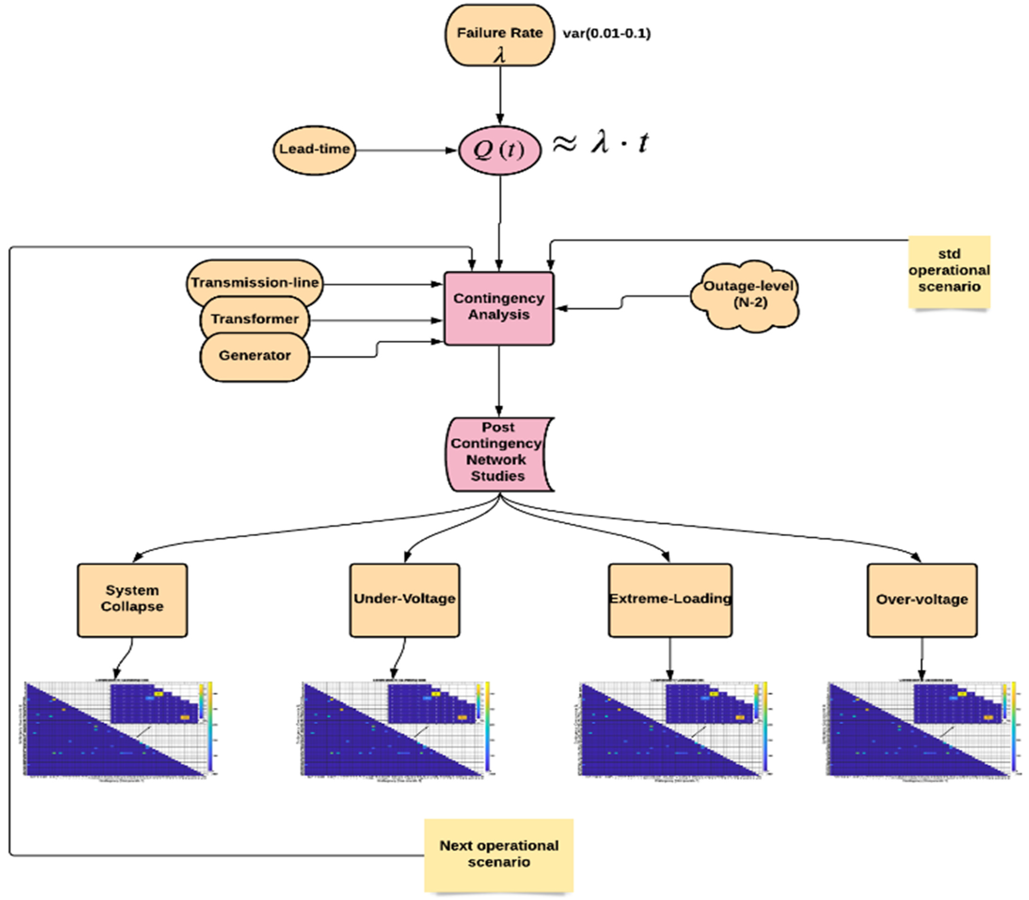
As depicted in Figure 1, after computation of the component unavailability, the probability of contingency is calculated and then contingency analysis is conducted, including all N-2 contingencies. In this study, failures of transmission lines, transformers and generators are considered for the contingency definition.

After performing contingency analysis, i.e., studying the transmission system for all cases when two components are unavailable, the impact of contingency cases is quantified in terms of severity factors. To calculate the severity factor $F_s\left(c\right),$ network studies are required [33]. In this study, four types of network studies are carried out, which correspond to four different severity factors.

• Overvoltage;
• Extreme loading;
• Undervoltage;
• System collapse.

For instance, the contingency (i.e., the loss of two components) will typically result in an increased loading for transmission lines and transformers; overload may occur because of this. The severity factor for extreme loading is quantified as the actual loading during the contingency case as a percentage of the component loadability. When the actual loading is less than the loadability, the severity factor equals zero. Otherwise, the severity factor is the actual loading value. This actual loading is considered in terms of a loading continuous (%L.C) which is the loading data given by the power-system analysis package Power-factory. A contingency case may also result in overvoltage or undervoltage. The severity factor for undervoltage or overvoltage is quantified as the voltage step, i.e., the difference between the base voltage (voltage before the contingency) and the voltage at different buses during the contingency. The voltage step is expressed in per-unit (p.u.). The severity factor for system collapse is quantified through non-convergent contingency cases and expressed as a percentage (%).

2.3. Quantifying the Operational Risk

The following general definition of operational risk is used in this study (7):

$$R_{op}={\displaystyle \sum }_{c=1}^{N_c}\Delta R_{op}\left(c\right)$$

(7)

where the contribution of a contingency $c$ to the operational risk is expressed as:

$$\Delta R_{op}\left(c\right)=P\left(c\right)\times F_s\left(c\right)$$

(8)

By obtaining $P\left(c\right),$ i.e., the probability of contingency from (6) and the severity factor,$F_s\left(c\right),$ from the Power-factory, the contribution of individual contingencies to the specified operational risk can be quantified.

2.4. Operational Scenarios

To illustrate the proposed methodology for presentation of the results from operational risk assessment, contingency analysis is performed on the IEEE 39-Bus sample network (refer to Figure S1) considering all (N-2) contingency cases. Four different types of network studies have been used to quantify the severity factor. This results in four different values for the operational risk, as in (7). For this network, by including all transmission lines, transformers and generators, the total number of components with non-zero unavailability is 56. The total number of (N-2) contingency cases for this network is 1540. Contingency analysis and various severity factor calculations are conducted using the power system analysis package “Power Factory”.

The following four operational scenarios have been considered in this study:

• Std-GLM as the first operational scenario (OS-1);
• 40% increment in GLM as a second operational scenario (OS-2);
• 60% increment in GLM as a third operational scenario (OS-3);
• 80% increment in GLM as a fourth operational scenario (OS-4).

Std-GLM (standard generation loading mix) is considered as a first operational scenario (OS-1) at which the generation loading level is at its nominal value “as defined in the IEEE 39-Bus system”. For the second operational scenario (OS-2), all generation and loading is increased by 40% and so on. Contingency analysis and network studies are performed for the considered operational scenarios and impacts of contingencies are analyzed.

3. Proposed Methods for Visualization of the Results

3.1. Data Resulting from Operational Risk Assessment

Operational risk assessment is primary aimed at obtaining a value for the operational risk, as defined in Section 2.3, for a specific operational state, for a specific system loading and for specific weather conditions. In the case where multiple severity factor definitions are used, multiple values for the operational risk will result. These values will next be compared with certain predefined thresholds for what is considered acceptable operational risk; based on this comparison, it is decided whether the operational risk is sufficiently low or too high. In the latter case, mitigation actions are needed to reduce the operational risk. Finding criteria for deciding when the operational risk is too high is one of the major challenges before application of operational risk assessment, but it is beyond the scope of this paper.

When the operational risk is too high, measures should be taken. With the classical deterministic approach (the (N-1)-criterion), a list would result of which contingency cases would make it so that the criterion was not valid. With operational risk assessment, there is no such list; instead, each contingency case with a non-zero severity factor contributes to the operational risk. The available data from the operational risk assessment is, as illustrated by (7) and (8), not just the operational risk, but also

• The probability of occurrence of the contingency case;
• Severity factor or factor quantifying the impact of the contingency case;
• Contribution to the operational risk of each contingency.

It is this data this is available to the TSO. It can be used, among others, to decide on a mitigation action, i.e., on a method to reduce the operational risk. These data can also be used to obtain suitable threshold values for acceptable operational risks. This can be achieved by gradually obtaining experiences and determining what are the actual values of the operational risk experiences by the transmission system and what are the contributions of individual components and contingencies to this. The detailed information can also be used to make case-by-case comparisons of the impact on operational risks by taking specific mitigation actions, i.e., impacting either the probability or severity factor for specific contingencies.

In this paper, two different ways of presenting that detailed data visually are proposed. One of those (presented in Section 3.2) shows the contribution to the operational risk for all (N-2) contingency cases; the other one (presented in Section 3.3) plots probability against severity factor for each of the contingency cases included in the operational risk. This chart enables a comparison of severity factor and probability between the different contingency cases. When there are multiple severity factor definitions, two such charts will result for each definition. This is illustrated in Section 4.

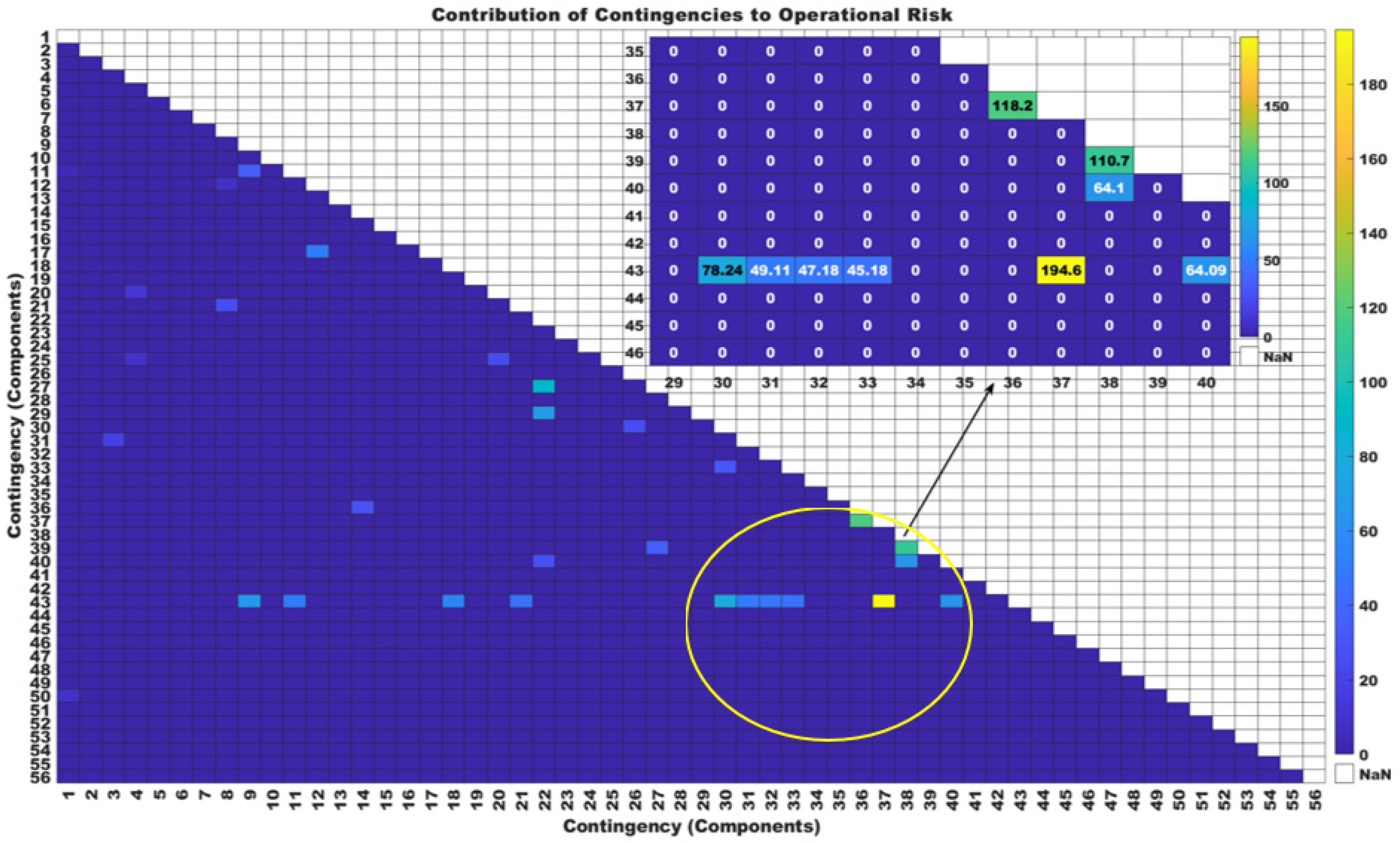
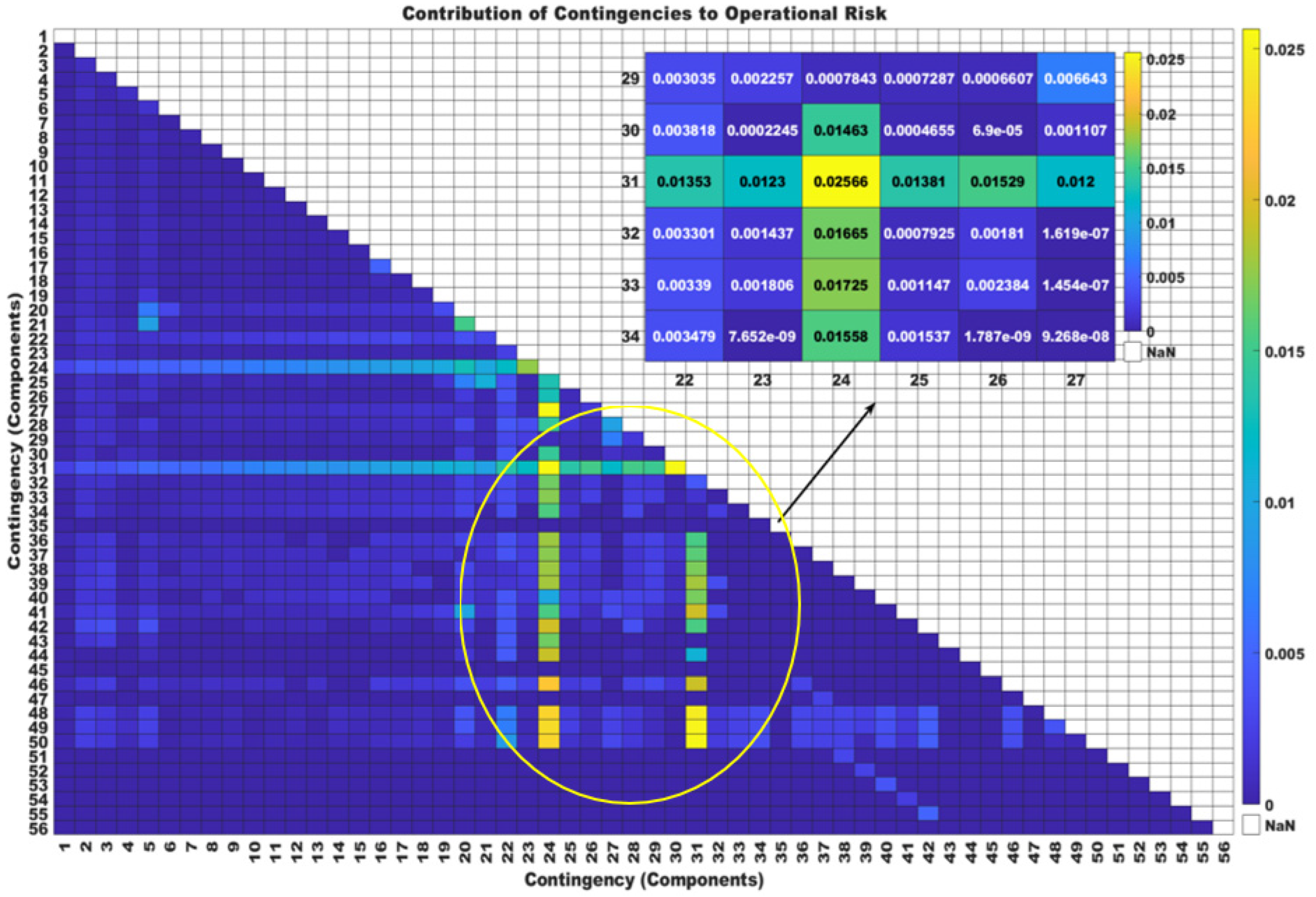
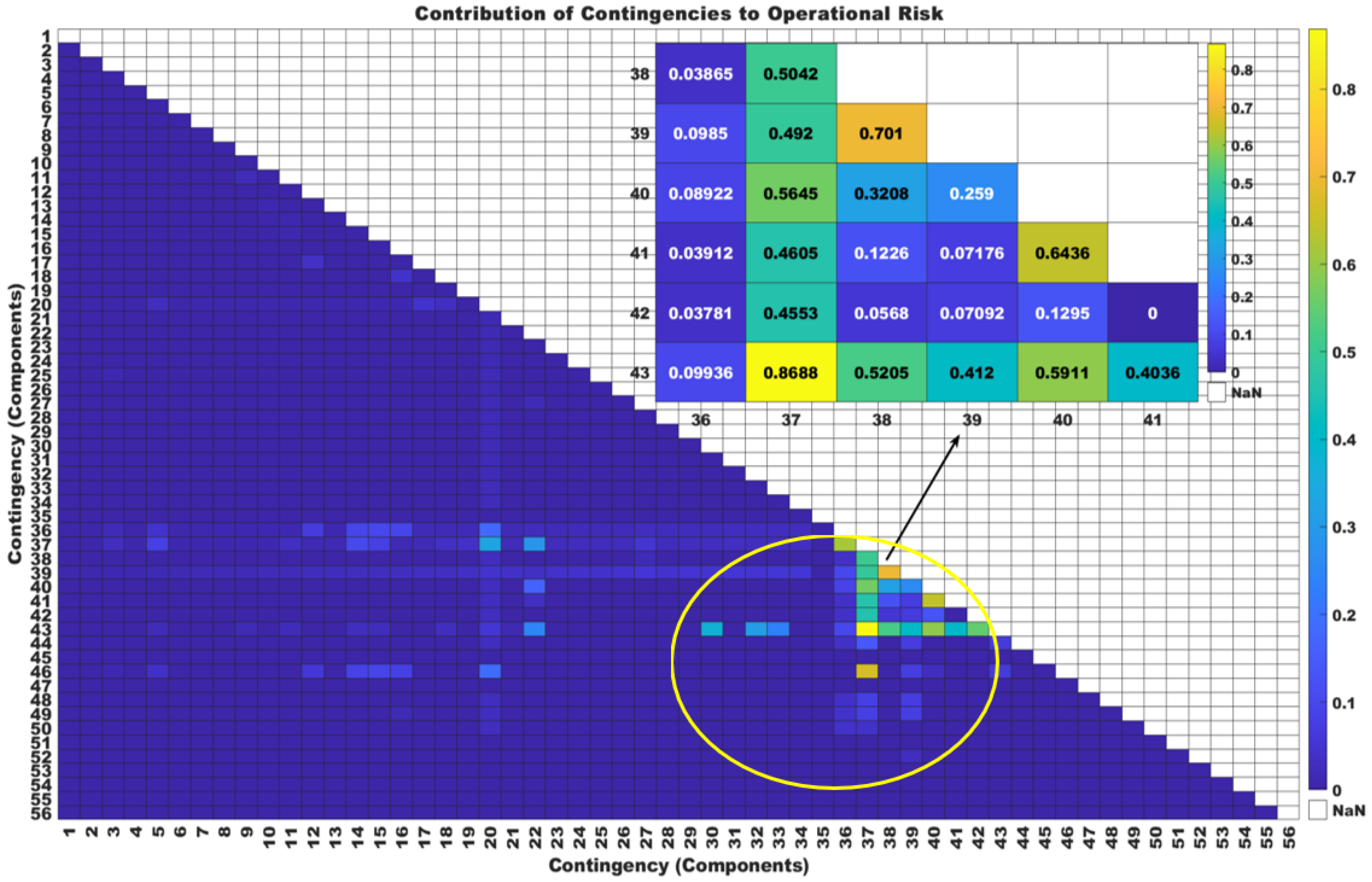
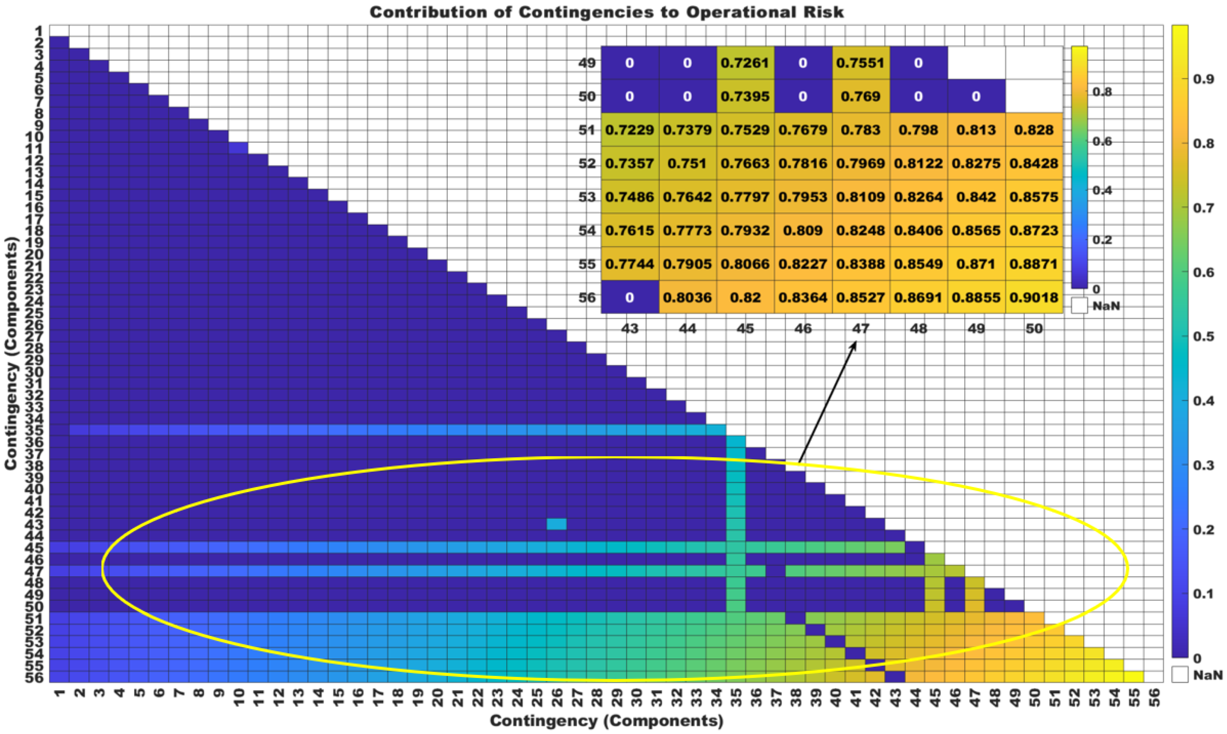
3.2. Contribution of Contingencies Visualization through Heat-Map

One way to visualize the operational risk results from the individual contribution of each contingency case is to present them through a heat-map. The map covers all (N-2) contingency cases, where the different system components are associated with the horizontal and vertical axis. In this study, the component outage order is ignored so the contingency case (1, 2) or (2, 1) is the same. As a result, only one-half of the map is needed. The diagonal cells, such as (1, 1) or (2, 2), could be used for the (N-1) contingency cases, but these are not considered in this study. By deploying (8), the contribution of each contingency case to the operational risk is quantified and represented in this map through a color bar. In addition, through this map, the TSO can envision which contingency is most jeopardizing to the operational security of the system; i.e., which one is contributing most towards the operational risk.

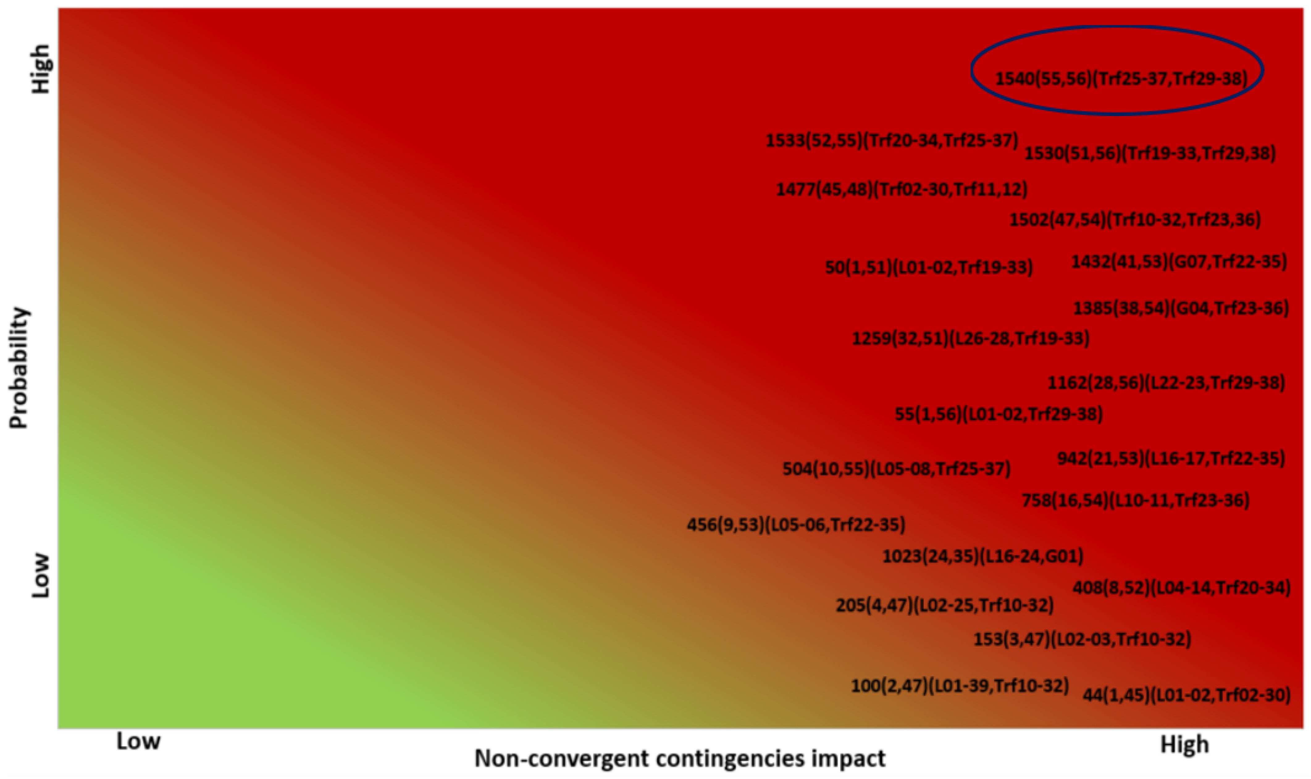
3.3. Contingencies Analysis through Risk-Based Contingency Chart

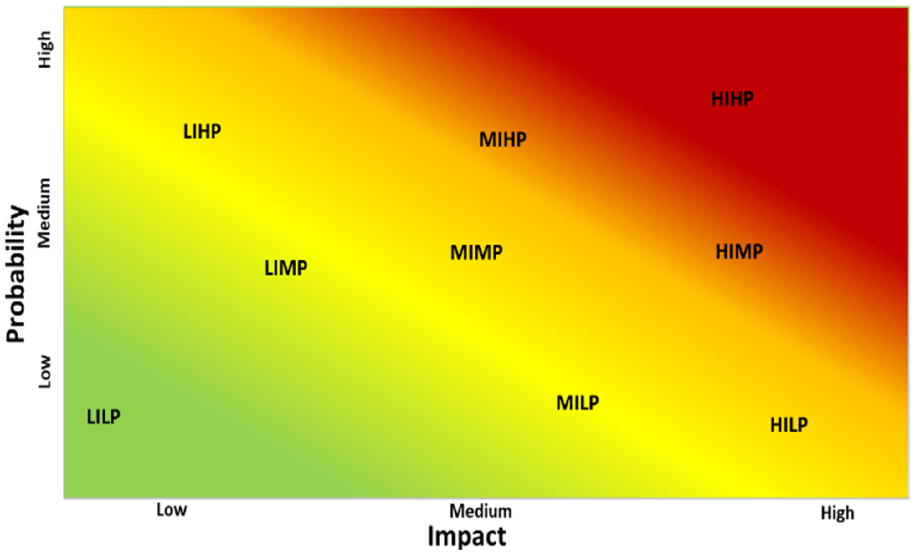
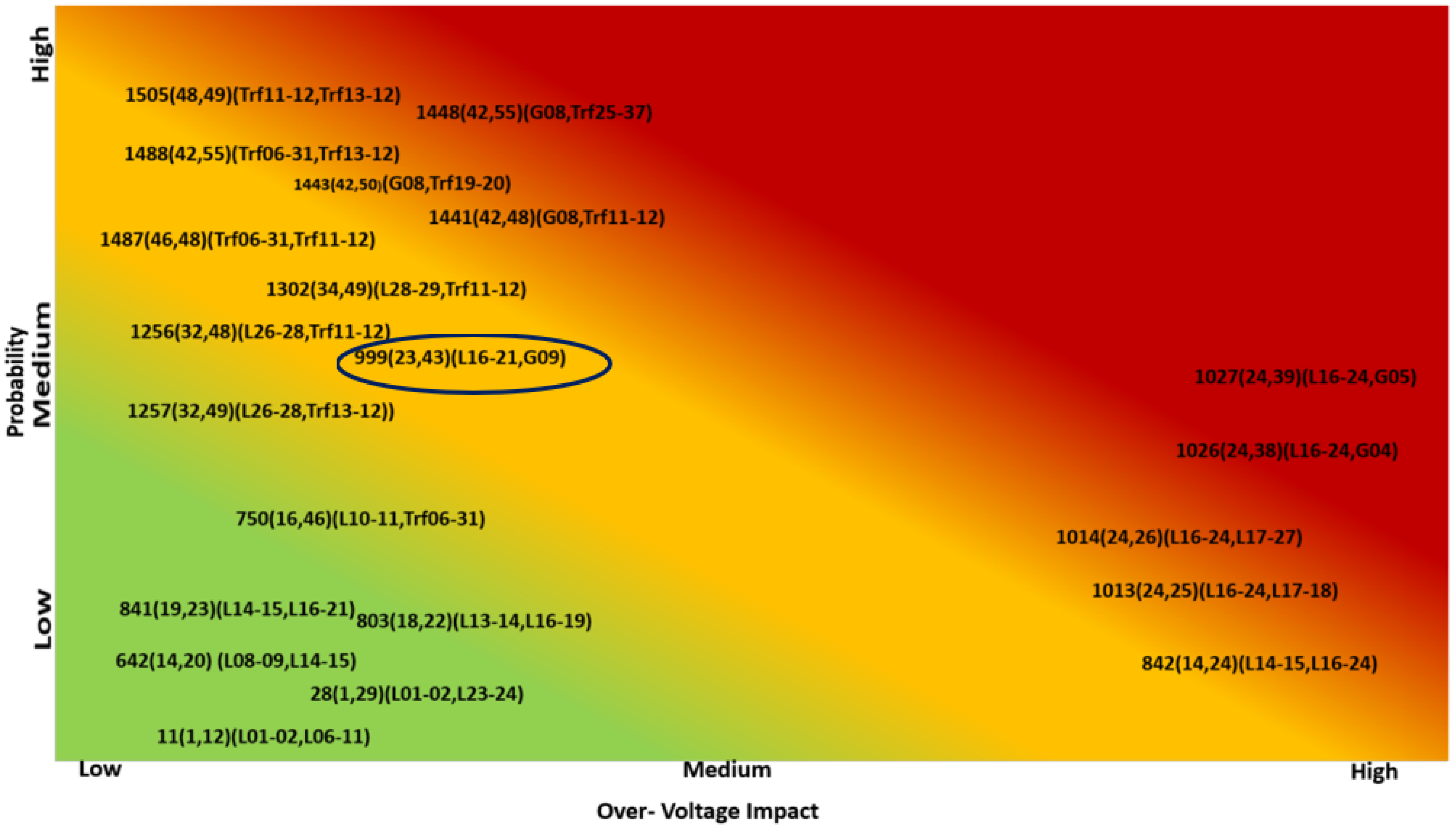
An alternative way of presenting the results of operational risk assessment from the contingencies aspect is by plotting probability against impact (severity factor) for the contingency cases. An example of the resulting chart is shown in Figure 2. This graphical presentation allows a distinction between different types of contingency cases based on impact and probability. A possible further classification would be as follows:

• LIHP (low impact high probability);
• MIHP (medium impact high probability);
• HIHP (high impact high probability);
• LIMP (low impact medium probability);
• MIMP (medium impact medium probability);
• HIMP (high impact medium probability);
• LILP (low impact low probability);
• MILP (medium impact low probability);
• HILP (high impact low probability).

This risk-based contingency chart helps the TSOs to compare the contingency cases based on impact (severity factor) and probability. This helps the operator to identify which contingency cases contribute most towards the operational risk. The “high” and “low” values along the vertical and horizontal axes are relative for the contingency cases with just the specific operational, loading and weather conditions. The absolute value of the total operational risk is compared with a threshold value, but once that comparison has been made, it is the relative values that matter for further decision-making.

In the above risk-based contingency case chart, the green portion shows low impact low probability (LILP) contingency cases, the yellow portion depicts medium impact medium probability contingency cases (MIMP), and the top-most right corner depicts the most threatening contingency cases: high impact high probability (HIHP) contingencies.

Contingency cases in the red portion of the chart, i.e., HIHP, will make a major contribution to the operational risk and immediate mitigation actions may be needed for these contingencies. The transition of one contingency case from the green portion to red under different operational scenarios shows that the impact and/or the probability of occurrence of that contingency case are increasing. Even when contingencies only occur in the green part of the chart, the operational risk (the sum of all contributions) may still be high and may have to be included during the operational planning.

4. Practical Interpretation of Contingencies Pattern and Its Contribution towards Operational Risk

The visual representation of operational risk in terms of the contribution of the contingency case to the specified risk through heat-map is discussed in this section. A contingency case under the probability and impact aspect is analyzed for four different types of operational risk.

4.1. Operational Risk of Extreme Loading (OREL)

OREL quantifies the risk that contingency cases create extreme loading situations for transformers and transmission lines. As mentioned in Section 2.2, the severity factor of an extreme loading case is calculated as the actual loading in terms of percentage of loadability.

Extreme loading is, in this study, defined as a situation in which the loading of a line or transformer exceeds the loadability as defined in the IEEE 39-Bus network. During the lead-time, if one contingency creates extreme loading for multiple components, then the severity factor is the absolute sum of the loading values for those components. If no component crosses this limit, then the severity factor for this contingency is zero. Operational risk result visualization from the contingency aspect from different methods is presented in this section for the first operational scenario (STD: GLM). Visualization of the results for the other operational scenarios is presented in an appendix.

4.1.1. Visualization through Heat-Map

The heat-map for the first operational scenario, using OREL, is shown in Figure 3. Even for the first operational scenario (OS–1), several contingencies contribute highly to the OREL. Contingency number 1356 (involving components 37 and 43) gives the highest contribution, 194.6%. When component 37 (generator G-03) and component 43 (generator G-09) are both unavailable, this results in 358.8% loading continuous value for the transformer (06-31) between Bus-06 and Bus-31. Similarly, contingency number 1331 (36, 37) gives 118.2% contribution towards the OREL. The occurrence of contingency 1331, when component 36 (generator G-02) and component 37 (generator G-03) are unavailable, creates extreme loading for two components simultaneously: 128.1% for (Line 08–09) and 126.8% for (Line 09–39). The resulting severity factor is 254.9%. The probability of occurrence of this contingency case is 0.4636. Consequentially, the contribution of this contingency case to the operational risk is 118.1%. The highly contributing contingencies are represented by the large yellow circle in Figure 3. This heat–map allows for an easy identification of the contingency cases and components that contribute most to the operational risk.

The heatmap that depict the contribution of extreme loading contingencies for other operational scenario e.g., during which the generation loading levels is at 40%, represented in Figure S2, at which the maximum contribution of contingency case reaches up to 641.5%. Figure S3 represents the contribution of extreme loading contingencies at 60% generation loading level. Figure S4 represent the contribution of extreme loading contingencies at 80% generation loading level. At this operating condition the contribution of contingency reaches up to 621.9%.

4.1.2. Risk-Based Contingency Chart

The second way to visualize operational risk is via a “Risk-based contingency chart”, which shows, for individual contingency cases, both the probabilistic and impact aspect. Figure 4 represents the risk-based contingency chart for OREL case, for the (OS-1) first operational scenario. In the figure, LILP, MILP, HILP, HIHP, MIHP and MIMP contingency cases can be noticed. For instance, contingency 1356 (component 37 (G03) and 43 (G09)) appears in the high impact high probability (HIHP) region. On the other hand, contingency 555 (component 12 (L06–11) and 17 (L10–13)) appears in the high impact low probability (HILP) part of the chart. Contingency case 1370 (G04, G05) appears in the medium impact high probability (MIHP) part of the chart. Contingency 1407 (G06, G09) and 1079 (L17–27, L25–26) fall in the medium impact medium probability (MIMP) region.

Risk based contingency charts for operational risk of extreme loading (OREL) under different operational scenario e.g., for 40%, 60%, 80%, generation loading level are shown in Figures S5–S7 respectively. For instance, Figure S5 represent risk-based contingency chart at 40% generation loading level and depict that at this operational scenario mainly LILP, MIMP and HIHP contingency cases can be noticed. Figure S6 represent the extreme-loading risk-based contingency chart at 60% generation loading level at which mainly LILP and MIMP contingency cases can be noticed. Figure S7 shows the extreme-loading risk-based contingency chart at 80% generation loading level at which LILP and HIHP contingency cases can be observed.

4.2. Operational Risk of Overvoltage (OROV)

OROV quantifies the operational risk that contingency cases create an overvoltage problem. As discussed in Section 2.2, the severity factor for overvoltage is calculated in terms of voltage step (p.u.); the difference between the voltage during and before the contingency. Overvoltage in this study is defined as a situation in which the busbar voltage exceeds the threshold set to 1.05 p.u. If multiple busbars experience overvoltage, then the severity factor is the absolute sum of the voltage steps. Otherwise, the severity factor for the contingency case is zero. In short, each bus with overvoltage during a contingency case contributes with their voltage change to the severity factor. The nominal voltage range is set between 0.95 p.u. and 1.05 p.u.

4.2.1. Visualization through Heat-Map

The contribution of all (N-2) contingencies towards the OROV is represented in Figure 5. During the first operational scenario (OS-1), mainly components number 31 (Line 26–27) and 24 (Line 16–24) contribute to this risk, depicted through the large circle in Figure 5. For instance, contingency numbers 1232 (31, 48); 1233 (31, 49); 1234 (31, 50); 1019 (24, 31); 1190 (30, 31); and 1015 (24, 27) contribute highly towards the OROV.

These contingencies contribute highly towards the OROV because they create serious overvoltage at multiple buses. For instance, contingency 1232 (31, 48) creates a voltage of 1.074 p.u. at Bus 26, 1.065 p.u. at Bus 25, 1.064 p.u. at Bus 36, 1.061 p.u. at Bus 28 and 1.058 p.u. at Bus 29. Similarly, for contingency 1015 (24, 27), component 24 (Line 16–24) and component 27 (Line 21–22) result in voltages of 1.094 p.u. at Bus 24; 1.071 p.u. at Bus 22; 1.068 p.u. at Bus 23; 1.064 p.u. at Bus 36.

The heat-maps that depict the contribution of overvoltage contingencies for other operational scenario e.g., during which the generation loading level at 40%, is represented in Figure S8 at which many contingency cases are taking high contribution towards the operational risk of overvoltage. Figure S9 represent the heat–map for operational risk of overvoltage at 60% generation loading level, at this operational scenario less number of contingencies are contributing as compared to the previous operational scenario, but with high contribution. Figure S10 represent the overvoltage contingency contribution at 80% generation loading level at this operating condition few contingencies are taking part in operational risk of overvoltage.

4.2.2. Risk-Based Contingency Chart

The risk-based contingency chart for OROV during operational scenario 1 (OS-1) is shown in Figure 6. For instance, for contingency case 842, in which component 14 (L14–15) and component 24 (L16–24) are unavailable, 1013 (24, 25) and 1014 (24, 26) fall in the high impact low probability (HILP) area of the chart. The contingency cases 750 (16, 46), 841 (19, 23), 803 (18, 22), 642 (14, 20), 28 (1, 29) and 11 (1, 12) fall in the low impact low probability (LILP) portion of the chart. On the other hand, contingency cases 1257 (32, 49), 999 (23, 43), 1256 (32, 48) and 1302 (34, 49) fall in the low impact medium probability (LIMP) part of the chart. The contingency cases 1026 (24, 38) and 1027 (24, 39) would be classified as high impact medium probability (HIMP), and contingency 1448 (42, 55) and 1441 (42, 48) would be classified as medium impact high probability (MIHP) contingency cases.

Risk based contingency chart for operational risk of overvoltage (OROV) under different operational scenario is discussed in supplementary material from. For instance, Figure S11 represent the overvoltage risk-based contingency chart at 40% generation loading level at which mainly LILP and MIMP contingency case can be noticed. Figure S12 represent the overvoltage risk-based contingency chart at 60% generation loading level where mainly LILP and LIHP contingency case be observed. Figure S13 represent the overvoltage risk based contingency chart under 80% generation loading level where LILP, MIMP and HIHP contingency cases be noticed.

4.3. Operational Risk of Undervoltage (ORUV)

ORUV quantifies the operational risk that contingencies result in an undervoltage. In the same way as for overvoltage, the severity factor for undervoltage is calculated from the voltage step (p.u.). In the undervoltage case, the voltage step at a busbar is the difference between the voltage during the contingency case and the voltage before the contingency case. Undervoltage in this study is defined as a situation in which the voltage at a busbar is less voltage than the undervoltage threshold, set to 0.95 p.u. During the contingency, if multiple busbars experience undervoltage, then the severity factor is the sum of the voltage steps.

4.3.1. Visualization through Heat-Map

Figure 7 shows the heat-map for ORUV during the first operational scenario (OS–1). The map shows that the contingencies cases in which component numbers 37, 38 and 43 are involved (large yellow circle) contribute highly towards the ORUV. For instance, contingency cases 1356 (37, 43); 1370 (38, 39); 1359 (37, 46); and 1374 (38, 43) have the biggest contribution to the ORUV. For instance, contingency case 1356 (37, 43) has a high probability of occurrence, 0.5425, and has a high severity factor. Consequentially, the contribution of this contingency case is high. Contingency case 1356 results in undervoltage of 0.815 p.u. at Bus 32, 0.855 p.u. at Bus 12, 0.859 p.u. at Bus 07, 0.863 p.u. at Bus 08, 0.864 p.u. at Bus 06 and 0.865 p.u. at Bus 05, etc.

Likewise, in contingency 1370 (38, 39), component 38 (generator G-04) and component 39 (generator G-05) create undervoltage for different buses. For instance, Bus 34 experiences 0.802 p.u., Bus 20 experiences 0.809 p.u., Bus 33 experiences 0.831 p.u. and Bus 19 experiences 0.881 p.u. The probability of occurrence and the severity factor are both high. Thus, the contribution of this contingency is also high.

The heat-map that depict the contribution of undervoltage contingencies for other operational scenario e.g., during which the generation loading level at 40% is represented in Figure S14 in which many contingency cases are taking contribution to the operational risk of undervoltage. Figure S15 represent the contribution of undervoltage contingency at 60% generation loading level. This figure depicts as the generation loading level increases the more number of contingency cases are taking contribution towards the operational risk of undervoltage. Figure S16 represent the contribution of undervoltage contingencies at 80% generation loading level. At this operational scenario the contribution of individual contingency reaches up to the 2.062 (p.u.) represented in Figure S16.

4.3.2. Risk-Based Contingency Chart

The risk-based contingency chart for ORUV during the first operational scenario (OS-1) is shown in Figure 8. For instance, contingencies 19 (1, 20), 36 (1, 37), 126 (3, 20), 35 (1, 36), 145 (3, 39), 423 (9, 20), 392 (8, 36) and 440 (9, 37) fall in the low impact low probability (LILP) area in the chart.

On the other hand, contingency cases 740 (16, 36), 710 (15, 46) and 1024 (24, 36) fall in the medium impact medium probability (MIMP) portion of the chart. Contingencies 1359 (37, 46), 1436 (42, 43), 1405 (40, 41) and 1370 (38, 39) fall in the high impact high probability (HIHP) portion of the chart.

Risk based contingency chart for operational risk of undervoltage under different operational scenario is discussed in supplementary material. For instance, Figure S17 represent the undervoltage contingency chart at 40% generation loading level where mainly LILP, MIMP and HIHP contingency cases can be observed. Figure S18 represent the undervoltage risk-based contingency chart for 3rd operational condition at which generation loading level is 60%. At this operational condition mainly LILP, LIMP, LIHP and MILP contingency cases can be observed. Figure S19 represent the undervoltage risk-based contingency chart at 80% generation loading level. Mainly the contingency cases fall in LILP, LIMP, and LIHP region (refer to Figure S19).

4.4. Operational Risk of System Collapse (ORSC)

ORSC quantifies the operational risk that contingencies cause a system collapse. This is the most threatening situation for the transmission system operational security. In this study, ORSC is calculated through non-convergent contingency cases. For the non-convergent contingency cases, the severity factor is unified. Otherwise, the severity factor is zero.

4.4.1. Visualization through Heat-Map

The contribution of all N-2 non-convergence contingencies towards the ORSC is represented in Figure 9. During the first operational scenario (OS–1), multiple contingency cases contribute to the ORSC. For instance, contingency cases 1540 (55, 56), 1539 (54, 56), 1538 (54, 55), 1537 (53, 56), 1536 (53, 55), 1535 (53, 54) and 1534 (52, 56) contribute highly. The SF for the non-convergent contingency case is one. Consequentially, in ORSC, the contingencies contribute based on their probability of occurrence and the number of non-converging contingency cases.

ORSC contingencies behavior for other considered operational scenarios is discussed in the appendix.

The heat-map that depict the contribution of system collapse contingencies for other operational scenario e.g., during which the generation loading level is at 40%, represented in Figure S20. Many contingency cases are taking contribution in operational risk of system collapse. Figure S21 represent the contribution of system collapse contingencies at 60% generation loading level. Figure S22 represents the contribution of system collapse contingencies at 80% generation loading level. From these figures it can be observed that as the generation loading level increases the more number of contingency cases are taking contribution towards the operational risk of system collapse.

4.4.2. Risk-Based Contingency Chart

The SF for ORSC has only the values zero or one; only contingencies with SF equal to one will end up in the risk–based contingency chart. The only difference between the contingency cases is their probability of occurrence. This makes this method of presenting less relevant for this operational risk definition; it becomes de facto a one-dimensional representation. For instance, contingency cases 44 (1, 45), 100 (2, 47), 153 (3, 47), 205 (4, 47), 408 (8, 52), 1023 (24, 35) and 456 (9, 53) fall in the high impact low probability (HILP) portion of the chart.

On the other hand, contingency cases 1540 (55, 56), 1533 (52, 55), 1530 (51, 56), 1477(45, 48), 1502 (47, 54) and 1432 (41, 53) depicted in Figure 10 fall in the high impact high probability (HIHP) area of the chart.

It can also be noticed that those specified contingencies that are taking part in ORSC will not contribute to the other types of operational risk used in this paper.

Risk based contingency chart for operational risk of system collapse under different operational scenario is discussed in Supplementary material. For instance, Figure S23 represent the system collapse risk-based contingency chart at 2nd operational scenario at which the generation loading level is 40%. Figure S24 represent the system collapse risk based contingency chart at 60% generation loading level, similarly Figure S25 represent system collapse risk-based contingency chart at 80% generation loading level. Mainly in all system collapse risk-based contingency charts, HILP, HIMP, HIHP contingency cases can be noticed.

5. Discussion

Operational risk assessment results in additional information that can be used to ensure secure operation of the transmission grid. Next to the operational risk, detailed information about individual contingencies results from the assessment. The heat-map indicates the contribution of each contingency case to the operational risk, under a given severity factor definition. The risk-based contingency chart highlights contingency cases for which the probability of occurrence and the impact (quantified by the severity factor) are both high. The proposed methods allow a system operator to analyze and categorize which contingency case has the highest priority for being avoided. This is relevant input when deciding about measures to ensure high operational security.

Some potential barriers are discussed below from the operational risk application point of view; these potential barriers need to be addressed in future studies.

5.1. Data Resulting from Operational Risk Assessment

The ultimate aim of the methods presented in the paper is to assist the TSO in selecting mitigation methods to reduce the operational risk of the transmission system. The graphical presentation of the results is just a first step, albeit an important first step. Further steps needed are to relate these charts to mitigation methods. The graphical presentation methods should be applied to actual operational states in existing transmission systems. Mitigation methods should be applied to study how these affect the charts and the total operational risk. First candidates for those mitigation methods could be those used to mitigate non-compliance with the (N-1)-criterion. From this experience, methods can be developed to propose or select appropriate mitigation methods using the charts. Obtaining this knowledge will require a large number of theoretical and practical studies, where the charts proposed in this paper will play an important role.

The heat-map, as proposed in this paper, is limited to second-order contingency cases. Adding single-order contingencies is straightforward; for example, by showing them along the diagonal axis of the heat-map. Results for third-order contingencies may be shown using a three-dimensional plot, but it will require specialized experience to interpret this one. Showing information on higher-order contingency cases becomes a major challenge and alternative methods are needed here. However, there are other challenges with including fourth- and higher-order contingency cases, like the very large number of cases, so that the representation of the detailed results may be a minor issue comparatively. The application of the risk-based contingency chart is not limited to any contingency order.

5.2. Continuous and Discrete Contingencies under the Integration of Intermittent Energy Resources

The integration of renewable energy resources (RER) is expected to increase further during the coming years [34,35,36,37]. This increases the complexity of the network in a number of ways.

New types of uncertainties are introduced by RER integration at transmission level, which impacts the operational risk assessment. Contingencies due to classical generation units are of a “discrete nature”; the units are available or non-available with possibly a small number of intermediate stages.

Contingency occurrence in, for example, a wind power plant would be a continuous phenomenon. Due to prediction errors, the production at the end of the lead-time is a random variable with a continuous distribution function. The challenge is to redefine the concept of contingencies, including both discrete and continuous ones for operational security purposes.

The methods proposed in this paper are confined to discrete contingencies. Alternative methods may be needed when prediction errors of RER have a non-negligible contribution to the operational risk. This will, for example, allow the TSO to better assess the importance of prediction errors in the operational security.

5.3. Standardization

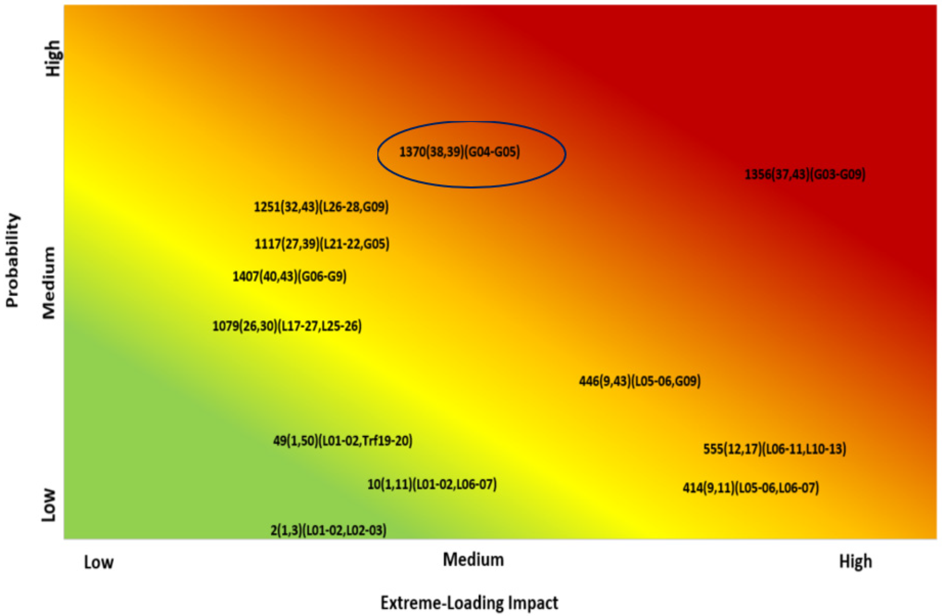
In the proposed risk-based contingency chart (Section 4, Figure 4, Figure 6, Figure 8 and Figure 10) each individual contingency case is characterized by its probability and impact. What has not been addressed here is what constitutes a high or low impact; similarly, what constitutes a high or low probability has not been addressed. The latter depends, among other factors, on what values are realistic for the component failure rate, a subject that was not addressed in this study. More experience is needed regarding calculations of operational risk for existing transmission systems. Interpretations of what is high and what is low may be conducted by an individual TSO. However, a better way forward would be for an international grid authoritative group to define this. Information on what is considered “high impact” and what is considered “high probability” is an important input to the TSO in deciding when measures are needed to increase operational security.

5.4. N-3 Contingencies Visualization and Fast Filtration

The proposed heat-map and risk-based contingency chart are based on parameters for all N-2 contingencies. When a fast decision has to be made in a large transmission system, it may not be possible to calculate these parameters for all (N-2) contingencies. Any of the filtration methods proposed in the literature may be used for this; both visualization methods can still be used even when not all (N-2) contingencies are available. The filtration methods may result in the need to include higher-order contingencies in the operational risk assessment. Including those in the risk-based contingency chart is straightforward, although the number of points may become large. Including (N-3) events in the heat-map is in theory possible by using a three-dimensional graph, but those are often difficult to interpret and information may easily be overlooked. Alternative methods need to be developed here, for example, by adding the contributions of all relevant (N-3) contingencies to an (N-2) contingency.

6. Recommendations

Operational risk assessment provides additional information on the operational security of a transmission system. However, there are some barriers against its widespread implementation by the TSOs. One of those is the absence of an acceptable risk level. Such an acceptable risk level could vary from grid to grid and may even be time-dependent within the same grid. To choose such a level, it is highly recommended to apply realistic operational risk assessment studies to realistic transmission systems using realistic component failure rates.

An international grid authoritative group should publish a recommended method, through which network studies should be conducted and post contingency impact can be quantified during operational risk assessment.

It is also recommended to propose and apply further methods in order to present and interpret the results from operational risk assessment of transmission systems.

7. Conclusions

Visualization of the results from operational risk assessment, using methods such as the ones proposed in this paper, could play a significant role in maintaining and improving the operational security of transmission systems. The incorporation of probabilistic behavior of contingency cases in operational security complements the existing deterministic methods for operational security. Visualization of contingency case contributions under the probabilistic aspect could depict which contingency cases contribute most towards the operational risk. In this study, this aspect is represented through a heat-map, which points out components that have a high contribution and to which special attention should be paid. Visualization of the results through a risk-based contingency chart incorporates the probability and impact of contingency cases in one chart. This helps to categorize contingency cases from both the probability and impact aspect. The two proposed visualization approaches have been illustrated for the IEEE 39-Bus test system for four different severity-factor definitions, under different operational scenarios.

Operational risk assessment, including the graphical methods proposed in this paper, allow the TSO to take preventive measures during or ahead of the lead-time by network reconfiguration, load reduction, etc., for better operational security.

References

1. Almeida, S.A.; Pestana, R.; Barbosa, M.F. Risk Assessment Methodology for Operations Aapplied to the Portuguese Transmission System—The Probabilistic Model. 2010. Available online: https://cigreindia.org/CIGRE%20Lib/CIGRE%20Session%202010%20paper/C2_212_2010.pdf (accessed on 20 June 2022).
2. Bollen, M.H.J.; Wallin, L.; Ohnstad, T.; Bertling, L. On Operational Risk Assessment in Transmission Systems–Weather Impact and Illustrative Example. In Proceedings of the 10th International Conference on Probablistic Methods Applied to Power Systems, Rincon, PR, USA, 25–29 May 2008. [Google Scholar]
3. Gjerde, O.; Vafeas, A.; Badajoz, C.; Quaranta, S.D. Generally Accepted Reliability Principle with Uncertainty Modelling and through Probabilistic Risk Assessment. 2013. Available online: https://cordis.europa.eu/project/id/608540 (accessed on 20 June 2022).
4. Kile, H. Generally Accepted Reliability Principle with Uncertainty Modelling and through Probabilistic Risk Assessment Project No: 608540; STATNETT SF: Oslo, Norway, 2013; Available online: https://prosjektbanken.forskningsradet.no/project/EU/608540?Kilde=EU&distribution=Ar&chart=bar&calcType=funding&Sprak=no&sortBy=date&sortOrder=desc&resultCount=30&offset=60&Geografi.1=S%C3%B8rTr%C3%B8ndelag&source=EU&projectId=608921.Accessed (accessed on 20 June 2022).
5. Kjølle, G.; Jakobsen, S.H. The GARPUR Project: Results and Recommendations towards Stakeholders. 2013. Available online: https://www.sintef.no/globalassets/project/garpur/deliverables/garpur-d9.1-recommendations-to-stakeholders.pdf (accessed on 20 June 2022).
6. Gjerde, O.; Wehenkel, L.; Vafeas, A. A New Approach to Reliable and Affordable Electric Supply in Europe. 2017. Available online: https://cordis.europa.eu/docs/results/608/608540/final1-d11-1d-garpur-final-report.pdf (accessed on 20 June 2022).
7. Rekinger, M.; Hofmann, M.; Chaouachi, A.; Karangelos, E.; Wehenkel, L.; Kjølle, G. The GARPUR Project: A Transition Roadmap towards Probabilistic Reliability Management. 2017. Available online: https://www.sintef.no/globalassets/project/garpur/deliverables/garpur-d9.2-transition-roadmap.pdf (accessed on 20 June 2022).
8. Geth, F.; Ergun, H.; Hertem, D.V.; Heylen, E. Generally Accepted Reliability Principle with Uncertainty Modelling and through Probabilistic Risk Assessment; Workshops Proceedings and Satisfaction Questionnaires. 2013. Available online: www.sintef.no/globalassets/project/garpur/deliverables/garpur-d10.3d-garpur-workshops-proceedings-all-rp.pdf (accessed on 20 June 2022).
9. Hamon, C.; Perkin, S.; Clement, R.; Tournebise, P.; Tabatabaeipour, S.M.; Silber, P.; Hering, P.; Khuntia, S.R.; Jose, J.L.; Rueda, L.; et al. How to Upgrade Reliability Management for Short-Term Decision Making. 2013. Available online: https://research.tudelft.nl/files/47535876/Khuntia_PhD_Draft_Thesis_Corrected_25Nov.pdf (accessed on 20 June 2022).
10. Haarla, L.; Mäkelä, O.; Brønmo, G.; Johansen, K.; Bach, P.F.; Kjølle, G. Current Practices, Drivers and Barriers for New Reliability Standards. 2014. Available online: https://www.sintef.no/globalassets/project/garpur/deliverables/garpur-d1.2-current-practices-drivers-and-barriers-for-new-reliability-standards.pdf (accessed on 20 June 2022).
11. Bollen, M.; Nazir, Z. Operational Risk Assessment–Time for a Smarter Look at Reliability for Power Transmission Systems; IEEE Smart Grid eBulletin. Available online: https://smartgrid.ieee.org/bulletins/june-2022/operational-risk-assessment-time-for-a-smarter-look-at-reliability-for-power-transmission-systems (accessed on 20 June 2022).
12. Nazir, Z.; Bollen, M.H.J. Operational Risk Assessment of Transmission Systems: A review 2022. Int. J. Electric. Power Energy Syst. 2022. submitted. [Google Scholar]
13. Regulation (EU) 2019/943 of the European Parliament and of the Council of 5 June 2019 on the Internal Market for Electricity. 2019. Available online: https://eur-lex.europa.eu/legal-content/EN/TXT/?uri=CELEX%3A32019R0943 (accessed on 20 June 2022).
14. ACER Decides Not to Approve ENTSO-E’s First Pan-European Resource Adequacy Assessment Due to Shortcomings. 2022. Available online: https://www.acer.europa.eu/events-and-engagement/news/acer-decides-not-approve-entso-es-first-pan-european-resource-adequacy (accessed on 20 June 2022).
15. Amendments to the Coordinated Security Analysis Methodology (SO GL Art. 75). 2020. Available online: https://consultations.entsoe.eu/system-operations/csam-amendments/ (accessed on 20 June 2022).
16. ACER Adopts Decision on Coordinated Security Analysis in Electricity. 2019. Available online: https://extranet.acer.europa.eu/Media/News/Pages/ACER-adopts-decision-on-coordinated-security-analysis-in-electricity.aspx (accessed on 20 June 2022).
17. Risk Preparedness: Proposal for Short-Term and Seasonal Adequacy Assessment Methodology. 2019. Available online: https://consultations.entsoe.eu/system-development/risk-preparedness-short-term-and-seasonal-adequacy/ (accessed on 20 June 2022).
18. Patton, A. Assessment of the Security of Operating Electric Power Systems Using Probability Methods. Proc. IEEE 1974, 62, 892–901. [Google Scholar] [CrossRef]
19. Patton, A. A Probability Method for Bulk Power System Security Assessment, I-Basic Concepts. IEEE Trans. Power Appar. Syst. 1972, PAS-91, 54–61. [Google Scholar] [CrossRef]
20. Mikolinnas, T.A.; Wollenberg, B. An Advanced Contingency Selection Algorithm. IEEE Trans. Power Appar. Syst. 1981, PAS-100, 608–617. [Google Scholar] [CrossRef]
21. Lauby, M.G.; Mikolinnas, T.A.; Reppen, N.D. Contingency Selection of Branch Outages Causing Voltage Problems. IEEE Power Eng. Rev. 1983, PER-3, 43–44. [Google Scholar] [CrossRef]
22. Capitanescu, F.; Glavic, M.; Ernst, D.; Wehenkel, L. Contingency Filtering Techniques for Preventive Security-Constrained Optimal Power Flow. IEEE Trans. Power Syst. 2007, 22, 1690–1697. [Google Scholar] [CrossRef]
23. Kaplunovich, P.; Turitsyn, K. Fast and Reliable Screening of N-2 Contingencies. IEEE Trans. Power Syst. 2016, 31, 4243–4252. [Google Scholar] [CrossRef]
24. Aboytes, F. Stochastic Contingency Analysis. IEEE Trans. Power Appar. Syst. 1978, PAS-97, 335–341. [Google Scholar] [CrossRef]
25. Shaalan, A.M. Contingency selection and ranking for composite power system reliability evaluation. J. King Saud Univ.-Eng. Sci. 2020, 32, 141–147. [Google Scholar]
26. Eftekharnejad, S. Selection of multiple credible contingencies for real time contingency analysis. In Proceedings of the 2015 IEEE Power & Energy Society General Meeting, Denver, CO, USA, 26–30 July 2015. [Google Scholar]
27. Amjady, N.; Esmaili, M. Application of a New Sensitivity Analysis Framework for Voltage Contingencies Ranking. IEEE Trans. Power Syst. 2005, 20, 973–983. [Google Scholar] [CrossRef]
28. Nan, L.; Liu, Y.; Wu, L.; Tianqi, L.; He, C. Graph Theory Based N−1 Transmission Contingency Selection and Its Application in Security-Constrained Unit Commitment. J. Mod. Power Syst. Clean Energy 2021, 9, 1458–1467. [Google Scholar] [CrossRef]
29. Aliyan, E.; Aghamohammadi, M.; Kia, M.; Heidari, A.; Shafie-khah, M.; Catalão, J.P. Decision tree analysis to identify harmful contingencies and estimate blackout indices for predicting system vulnerability. Electr. Power Syst. Res. 2020, 178, 106036. [Google Scholar] [CrossRef]
30. Preece, R.; Adrees, A.; Milanović, J.V. Risk-based framework for establishing and visualising operational constraints of power systems. In Proceedings of the 2014 Power Systems Computation Conference, Wroclaw, Poland, 18–22 August 2014. [Google Scholar]
31. Sun, Y.; Overbye, T.J. Visualizations for Power System Contingencies Analysis Data. IEEE Trans. Power Syst. 2004, 19, 1859–1866. [Google Scholar] [CrossRef]
32. Mitra, J.; Benidris, M.; Nguyen, N.; Deb, S. A Visualization Tool for Real-Time Dynamic Contingency Screening and Remedial Actions. IEEE Trans. Ind. Appl. 2017, 53, 3268–3278. [Google Scholar] [CrossRef]
33. Nazir, Z.; Bollen, M.H. Investigating Various Severity Factor Behaviors for Operational Risk Assessment. Electricity 2022, 3, 325–345. [Google Scholar] [CrossRef]
34. Schaber, K.; Steinke, F.; Hamacher, T. Transmission grid extensions for the integration of variable renewableenergies in Europe: Who benefits where? Energy Policy 2012, 43, 123–135. [Google Scholar] [CrossRef] [Green Version]
35. Bollen, M.H.; Hassan, F. Integration of Distributed Generation in the Power System; IEEE Press: Piscataway, NJ, USA, 2011. [Google Scholar]
36. Vittal, V.; Ayyanar, R. Grid Integration and Dynamic Impact of Wind Energy, 1st ed.; Springer: New York, NY, USA, 2012. [Google Scholar]
37. Fox, B.; Bryans, L.; Flynn, D.; Jenkins, N.; Milborrow., D.; Malley, O.M.; Watson, R.; Anaya-Lara, O. Wind Power Integration: Connection and System Operational Aspects; IET: London, UK, 2014. [Google Scholar]
Figure 1. The procedural flow of operational risk under different operational scenarios.
Electricity 03 00023 g001
Figure 2. Risk-based contingency case chart.
Electricity 03 00023 g002
Figure 3. Contribution of contingencies towards OREL (OS-1). The color scale indicates the contribution of each contingency (defined by Equation (8)), as quantified by the color bar on the right, in the relevant unit. The color scale is selected such that the lowest value is dark blue and the highest value is yellow.
Electricity 03 00023 g003
Figure 4. Risk-based extreme-loading contingency chart. For example, contingency number 1370 (indicated) in which the component number 38 (G-04) and component number 39 (G-05) are involved falls in the medium impact high probability (MIHP) region.
Electricity 03 00023 g004
Figure 5. Contribution of contingencies towards OROV (OS-1). The color scale indicates the contribution of each contingency (defined by Equation (8)), as quantified by the color bar on the right, in the relevant unit. The color scale is selected such that the lowest value is dark blue and the highest value is yellow.
Electricity 03 00023 g005
Figure 6. Risk-based overvoltage contingency chart. For example, contingency number 999 (indicated) in which the component number 23 (L16–21) and component number 43 (G09) are involved fall in the medium impact medium probability (MIMP) area.
Electricity 03 00023 g006
Figure 7. Contribution of contingencies towards ORUV (OS-1). The color scale indicates the contribution of each contingency (defined by Equation (8)), as quantified by the color bar on the right, in the relevant unit. The color scale is selected such that the lowest value is dark blue and the highest value is yellow.
Electricity 03 00023 g007
Figure 8. Risk-based undervoltage contingencies chart. For example, contingency number 1359 (indicated) in which component number 37 (G-03) and component number 46 (Trf 06–31) fall in the high impact high probability (HIHP) region.
Electricity 03 00023 g008
Figure 9. Contribution of contingencies towards ORSC (OS–1). The color scale indicates the contribution of each contingency (defined by Equation (8)), as quantified by the color bar on the right, in the relevant unit. The color scale is selected such that the lowest value is dark blue and the highest value is yellow.
Electricity 03 00023 g009
Figure 10. Risk–based system collapse contingencies chart. For example, contingency number 1540 (indicated) in which component number 55 (Trf 25–37) and component number 56 (Trf 29–38) fall in the HIHP region.
Electricity 03 00023 g010
Publisher’s Note: MDPI stays neutral with regard to jurisdictional claims in published maps and institutional affiliations.