Development of Demand Factors for Electric Car Charging Points for Varying Charging Powers and Area Types

Abstract

With the increasing number of electric vehicles, the required charging infrastructure is increasing rapidly. The lack of historical data for the charging infrastructure compromises a challenge for distribution system operators to forecast the corresponding increase in the load demand. This challenge is characterised by two main uncertainties, namely, the charging power of the charging infrastructure and its location. Expectedly, the charging infrastructure is going to include varying charging powers and is going to be installed country-wide in different area types. Hence, this contribution sets to tackle these two uncertainties by developing demand factors for the charging infrastructure according to the area type. In order to develop the demand factors, a stochastic simulation tool for the charging profiles has been run for a simulation period of 5200 weeks (100 years) for six main charging powers and seven area types for up to 500 charging points. Thus, compromising a total of over 2.1 million simulated charging profiles. The resulting demand factor curves cover the charging powers between 3.7 kW and 350 kW with 1 kW steps for a total of 348 kW steps. Furthermore, they differ according to seven area types ranging from an urban metropolis to a rural village and are developed for up to 500 charging points. Consequently, the demand factor curves serve as a base to be used for the strategic grid planning of distribution power grids while taking the future development of the charging infrastructure into account.

1. Introduction

As part of the energy transition and the goal of achieving the climate targets, the electrification of various sectors continues to advance [1]. One of the sectors in which a massive emission reduction can be achieved is the mobility sector [2]. For successful electrification of the mobility sector, an expansion of the charging infrastructure for electromobility is necessary. This expansion increases the load on the power distribution grids. Therefore, strategic grid planning has the task of considering the impact of charging points (CPs) on load development [3].

The charging infrastructure can be divided into private charging points (prCPs) and public charging points (puCPs), each with different charging powers. In the context of this contribution, a prCP is a CP which can be accessed by a certain user or group of users [4], while a puCP can be openly accessed by anyone [5]. As for the prCPs, they are primarily connected to single- and two-family houses but also to multi-family houses and small businesses at the low-voltage (LV) level with charging powers up to 22 kW, whereas the connection of puCPs mainly takes place at grid nodes in the LV grid or also at hotspots with several puCPs in the medium-voltage grid up to 350 kW.

With the lack of comprehensive historical data about the charging behaviour and only a few pilot projects known to record the corresponding grid utilisation, strategic grid planning must rely on other tools to estimate the perspective grid utilisation of existing or future CPs. Therefore, it becomes essential to apply the established method of using so-called demand factors (DFs) to determine the power demand, similar to what can already be used for conventional loads as in [6]. The DF is defined as: “the ratio, expressed as a numerical value or as a percentage, of the maximum demand of an installation or a group of installations within a specified period, to the corresponding total installed load of the installation(s)” [7]. By applying this to the charging infrastructure, the installation would be the CPs of certain charging power in one of the area types mentioned later on. The DFs consider that not all loads have the maximum power demand at the same time because the power demand is distributed throughout the day. As for the power demand of the charging infrastructure, this means that many plug-in electric vehicles (referred to as electric vehicles (EVs) in the remaining of this contribution) are charged throughout the day and never all simultaneously. This consideration leads to a realistic estimation of the grid load and thus, avoids over-dimensioning of the grid resources, particularly transformers and lines. Hence, this contribution develops DF curves for the charging infrastructure, which can, later on, be implemented to determine the expected load demand.

Since the driving behaviour differs according to the area type, the charging behaviour can subsequently differ with respect to the area type. Therefore, this contribution determines DFs for different area types so that they can be used as required in the context of strategic grid planning.

A further factor influencing the charging behaviour is the available charging power at the CP. With the development in charging technologies, higher charging powers (fast chargers) are becoming available and are increasingly spreading in the grids [8]. Accordingly, this contribution develops DFs for charging powers, starting with the widely established slow charging powers of 3.7 kW and 11 kW. It then continues to present DF curves for the fast chargers with charging powers reaching up to 350 kW. This wide spectrum of DF curves enables the distribution system operator to apply the DF curve corresponding to the charging power in a certain grid.

With the increasing number of CPs, it becomes necessary to dimension the grids for the corresponding number of CPs, which could reach tens and hundreds. Hence, the DF values are developed for up to 500 CPs. In the context of strategic grid planning, these DFs can be applied equally for the different voltage levels as well as for the modelling and application of load management systems.

1.1. Novelty and Significance of Demand Factors

The idea of utilising the load profiles for the corresponding load type in the field of strategic grid planning has been established for a long time. These load profiles can either be synthesised, such as in [9], which proposes a bottom-up approach for the household loads in order to establish the load diagrams for a certain area. Another model for generating household load profiles is presented in [10], which relies on the load characteristic of the different household appliances. A similar approach has been performed by [11] to generate household load profiles. These approaches aim to generate either representative electric load profiles (e.g., [12]) or to determine the load demand for a certain area or grid. The common factor among these approaches is that they rely on their prior knowledge of the household loads, either by knowing the typical usage of the household appliances or by utilising historically collected measurement data. However, this is not the case when it comes to EVs.

The field of EVs is fundamentally no longer new when the technology is considered on its own. However, there is a little experience so far in the context of strategic grid planning, as the penetration of the charging infrastructure within the grids has not yet reached a level that is predicted in many scenarios for the development of electromobility [13,14,15].

Some pilot projects, such as in [16], have already determined when EVs charge simultaneously for ten households (single-family houses) with a total of 11 EVs. The associated charging points are connected to one line, and the power demand is measured in the period from June 2018 to October 2019. The results show that in 73% of the day, none of the EVs are charging, and only in 0.1% of the daytime, a maximum of five EVs are charging simultaneously. There is no point in time when six, seven, eight, nine, ten or all eleven EVs are charging simultaneously, which again argues for the use of DFs. For exactly this case of private use with either 3.7 kW, 11 kW or 22 kW charging powers, there are also already initial studies such as [17] that have scientifically investigated and determined the DFs for uncontrolled charging at prCPs. In addition, a distinction is made between the metropolitan, suburban and rural area types so that a differentiated consideration can already be made in practice.

A second use case is developed by [18], in which the driving and charging behaviours of EVs have been simulated. Even though the publication [18] follows an approach similar to the approach applied in the contribution in hand, the results are limited to the charging power of 11 kW and for up 100 EVs.

In the aforementioned studies, charging processes at prCPs are generally considered. However, since there is also an increasing expansion of puCPs, their corresponding load values must be analysed. In [19], for example, 50,000 charging processes at 1000 puCPs are analysed with regard to their time series and load profiles without determining their simultaneity. However, one of the main results is that the charging behaviour at the puCPs is influenced by time- and location-dependent factors as well as the individual days of the week. Furthermore, it is stated in [19] that the assumption of a DF = 1 in the context of strategic grid planning leads to an over-dimensioning of the grid resources, so it makes sense to consider certain simultaneities.

The aforementioned studies show that there are still no comprehensive DFs for different charging powers and different area types that can be used in strategic grid planning for dimensioning transformers and lines for different grid areas. Therefore, this contribution aims to fill this gap. In the following sections, DF curves for charging powers between 3.7 kW and 350 kW, as already established up to 150 kW in [20] for urban grids, are developed for a total of seven different area types. These can be used for strategic grid planning for the integration of prCPs and puCPs at different voltage levels.

This is important for several reasons. On the one hand, different DFs are required to dimension transformers and lines according to their thermal loading limits specified in [21,22,23]. In addition, the specified limits for the voltage within the grids must also be maintained according to [24]. Figure 1 shows this relationship graphically. For the dimensioning of the transformer, all loads within the grid are taken into account to calculate the DF over all the feeders. In contrast, for the dimensioning of the lines, only those loads are taken into account, which are located in the respective feeder. An alternative method for dimensioning the resources is the use of time series analysis. However, an evaluation according to [25] from the perspective of the transformers as well as from the perspective of the lines has shown that time-series analyses do not offer any advantages in the determination of the standard grid resources. Furthermore, it shows that at considerable additional cost for the time series analysis, the resulting power demands by charging infrastructure in the LV grids are at the same level as when applying DFs. Therefore, DFs for charging infrastructure can still be recommended for strategic grid planning.

1.2. Structure and Objective of the Work

This contribution aims to provide an instrument, which can be used by distribution system operators for strategic grid planning while considering the charging infrastructure. The goal here is to provide the DF curves that are required to calculate the corresponding power demand according to the nominal charging power of the infrastructure and to the specific grid area. The following new findings are provided in this contribution:

1.

Analysis of the driving behaviour in terms of:

• Day of the week
• Purpose of the trip
• Number of trips per day
• Distance of the trip

2.

Generation of weekly charging profiles depending on the available charging power and the specified area type

3.

Development of DF curves for:

• Six dominant charging powers: (3.7, 11, 22, 50, 150 and 350) kW
• Seven area types (specified in Section 2)
• 500 CPs

4.

Implementation of a curve-fitting algorithm for charging powers with 1 kW steps starting from 3.7 kW up to 350 kW

Section 2 begins by explaining the data basis used for the analyses. This initially concerns mobility data from Germany, but it can be assumed that the basic mobility behaviour will not differ fundamentally from other countries, and the results can, therefore, also be used in other European countries. Section 3 then describes, in detail, the method developed to determine the various DFs. First, the general assumptions are explained, followed by the calculation and simulation tool and the mathematical background. In Section 4, the results of the simulations are presented extensively for different area types and charging powers. Finally, Section 5 discusses the results by evaluating the influence of the framework conditions and by performing a sensitivity analysis against results published by other studies.

2. Database

The main objective is to simulate the typical charging behaviour of a large number of vehicle users. Extensive study results from [26,27] are available for this purpose. They essentially contain mobility data gathered from 316,000 individuals from 156,000 households. The database contains statistical data gathered from more than one million routes of conventional combustion vehicles. For further analyses, it is fundamentally assumed that the mobility behaviour will not change just because vehicles have a new drive system. Therefore, it may be assumed that the EVs will substitute internal combustion vehicles while maintaining the same driving behaviour in the future.

The mobility data introduced in [26,27] contains key data for the driving profiles. For example, Figure 2 shows how the mobility data differ in the number of daily routes (left) or the reason for the route (right). In addition, Figure 3 shows how the lengths of the routes (left) and departure times (right) differ for different reasons for the routes for the area type: Urban Region: Metropolis. The probability distributions for the six remaining area types are displayed in Appendix A.

The two studies from the year 2008 [26] and the year 2018 [27] differ not only in an update of the data but also in further differentiation of the area types. The differentiation introduces the following seven area types:

• Urban Region: Metropolis
• Urban Region: Regiopolis, Large City
• Urban Region: Medium-sized City, Urbanised Area
• Urban Region: Small-town Area, Village Area
• Rural Region: Central City
• Rural Region: Medium-sized City, Urbanised Area
• Rural Region: Small-town Area, Village Area

The seven area types are based on [29]. The distribution of the area types across the Federal Republic of Germany is shown in Figure 4. This shows the extent to which the above-mentioned differentiation of the area types is distributed geographically. This distribution is highly relevant in Section 3 and Section 4, as the DFs for these seven different area types are determined. Consequently, the distribution grid operators can classify themselves into one of the area types and then use the relevant DFs for their specific strategic grid planning.

3. Method

The following section describes, in detail, how the DFs for different area types are methodically generated. Starting with the general conditions, the simulation tool is then explained, which is then used to finally calculate the DFs.

3.1. General Conditions

In addition to the mobility data, which describe the driving profiles, further input data need to be assumed to specify the charging profiles in the simulation.

Firstly, the charging behaviour must be specified. Since, according to Section 1.1, there is limited comprehensive experience in dealing with charging processes, the so-called chaotic charging is assumed. As a further assumption, the battery consumption must be assumed as a basis for the calculations, as this also influences the charging periods. As the battery consumption increases, so does the probability of long charging times. In this context, the respective state of charge at the destination is taken into account so that, for example, longer driving distances result in a lower state of charge. When the battery’s state of charge reaches 100% during the charging process, the charging process is terminated. If the charging period for a 100% state of charge exceeds the parking period at a certain destination, the EV is charged until the parking period is over, and then it starts to move to the next destination. The priority is usually given to riding the EV rather than charging it.

For the analyses, an average battery capacity of 45 kWh and an average consumption of 20 kWh per 100 km are assumed per [20].

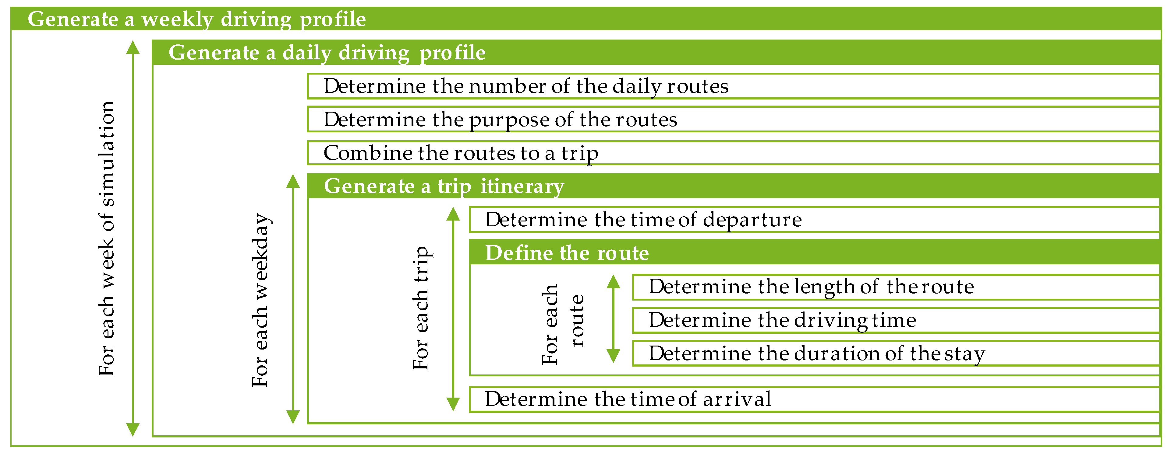
3.2. Simulation Tool

The simulation tool developed in [30] is used to generate driving profiles based on the mobility data from [26,27] and is developed in the programming software MATLAB. Figure 5 shows how weekly driving profiles are generated using the corresponding algorithm. First, the length of the route, the driving time, and the duration of stay are determined for each route. These defined routes are then consolidated into individual trip profiles by determining the departure and arrival times. Different trip progressions then generate a daily trip profile depending on the number of the daily routes and the purpose of each one of them. By generating the daily driving profiles, weekly trip profiles are generated. Finally, according to the generated driving profiles, charging profiles can be generated.

For the generation of the charging profiles, it is assumed that CPs are available at the destinations defined as the purpose of the route, which is given in Figure 2 and Figure 3. In addition, the charging of the EVs is assumed to mainly occur at the final destination of the EV (home charging). Nevertheless, the EV can be charged at one of the stops over the day (intermediate charging) according to a linear probability distribution corresponding to the state of charge. When the current EV range is shorter than 50 km, the probability of intermediate charging is maximised, whereas with an EV range longer than 150 km, the probability of intermediate charging is minimalised. The probability distribution then spreads the probability of intermediate charging according to the EV range linearly between these two values.

In case only one CP is available in the city, grid or area, this CP will be located at one of the above-mentioned destinations. Consequently, the EV(s) arriving at this specific destination can charge according to the assumed available charging power. This case leads to the following conclusions:

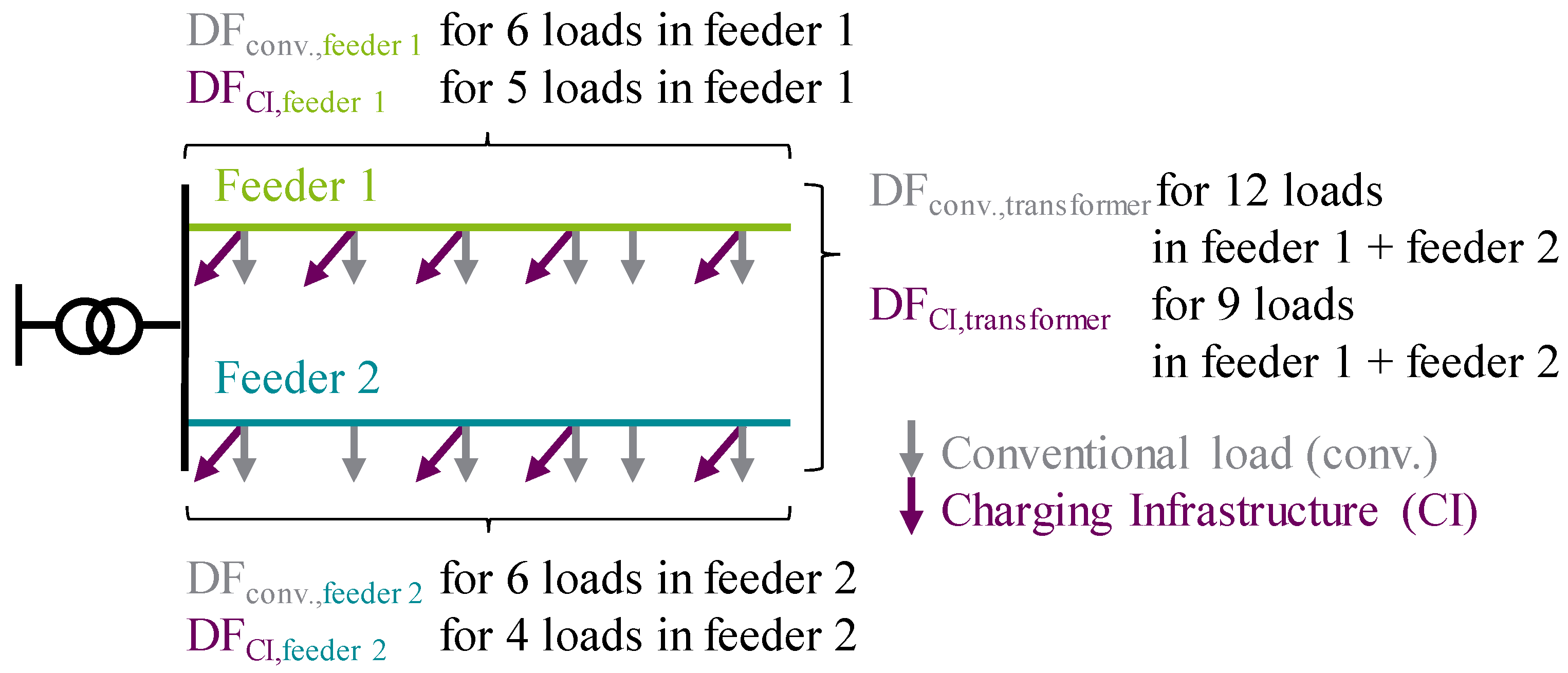
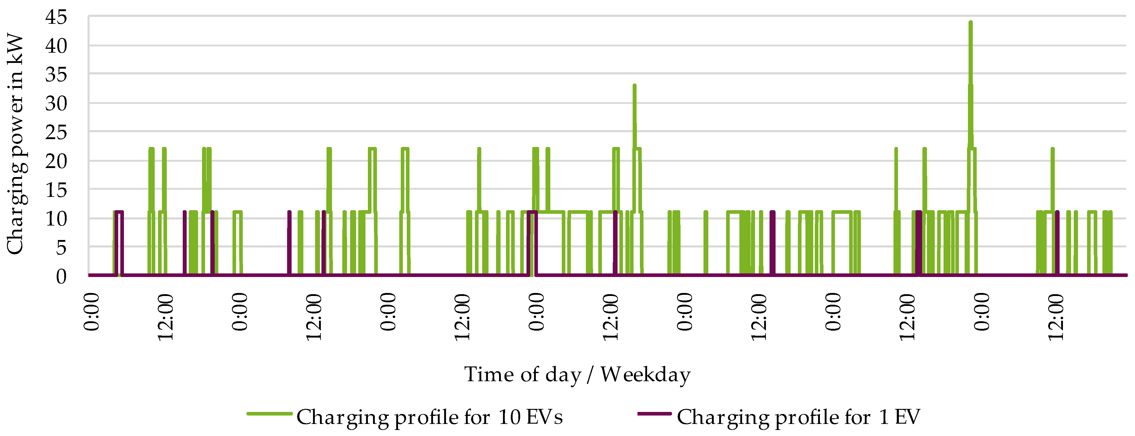
• Independent of the number of consecutive charging processes for the single CP (e.g., 10 EVs are charging after one another at the same single CP), the maximum power drawn simultaneously from the electric grid equals the nominal power of this single CP. Hence, the DF equals 1 (see Equation (1) in Section 3.3). Naturally, this situation does not apply if several CPs are available, which is the main investigation in the contribution. With the focus on strategic electric grid planning, the question that the contribution aims to answer is not how many EVs can be charged with a limited number of CPs but rather how many CPs are being used at the same time when there is unlimited access to CPs.
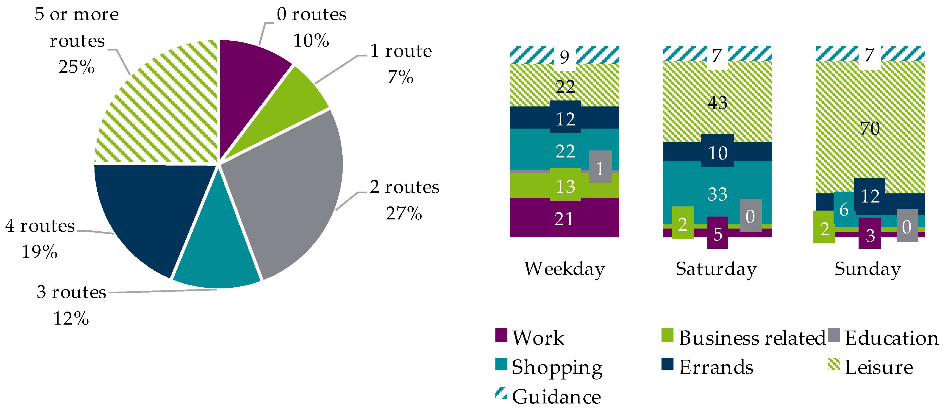
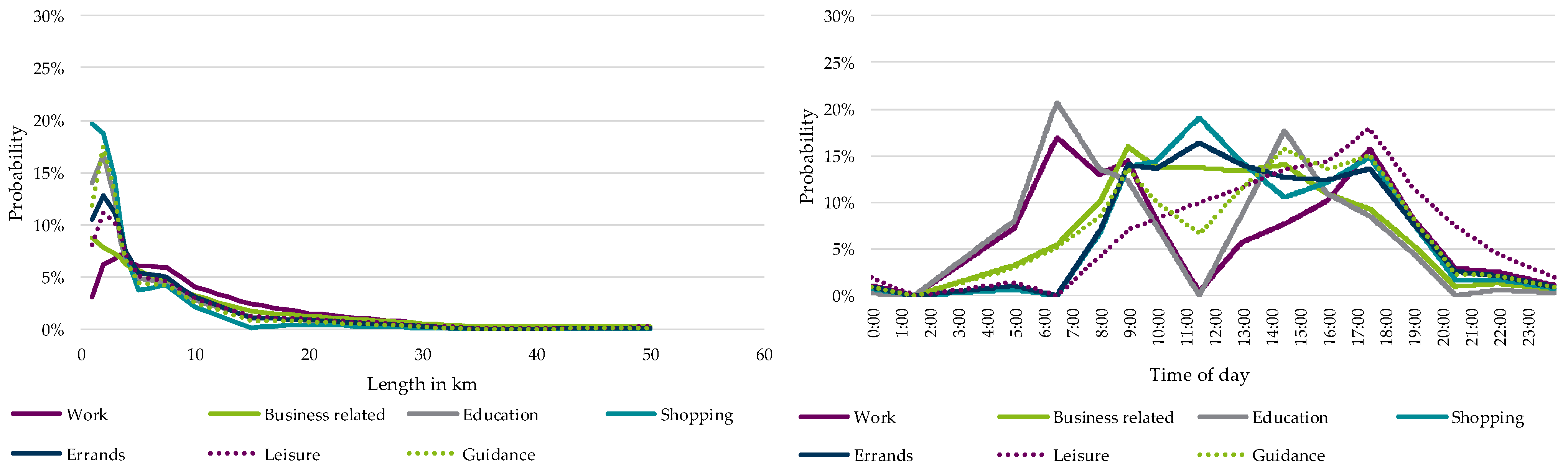
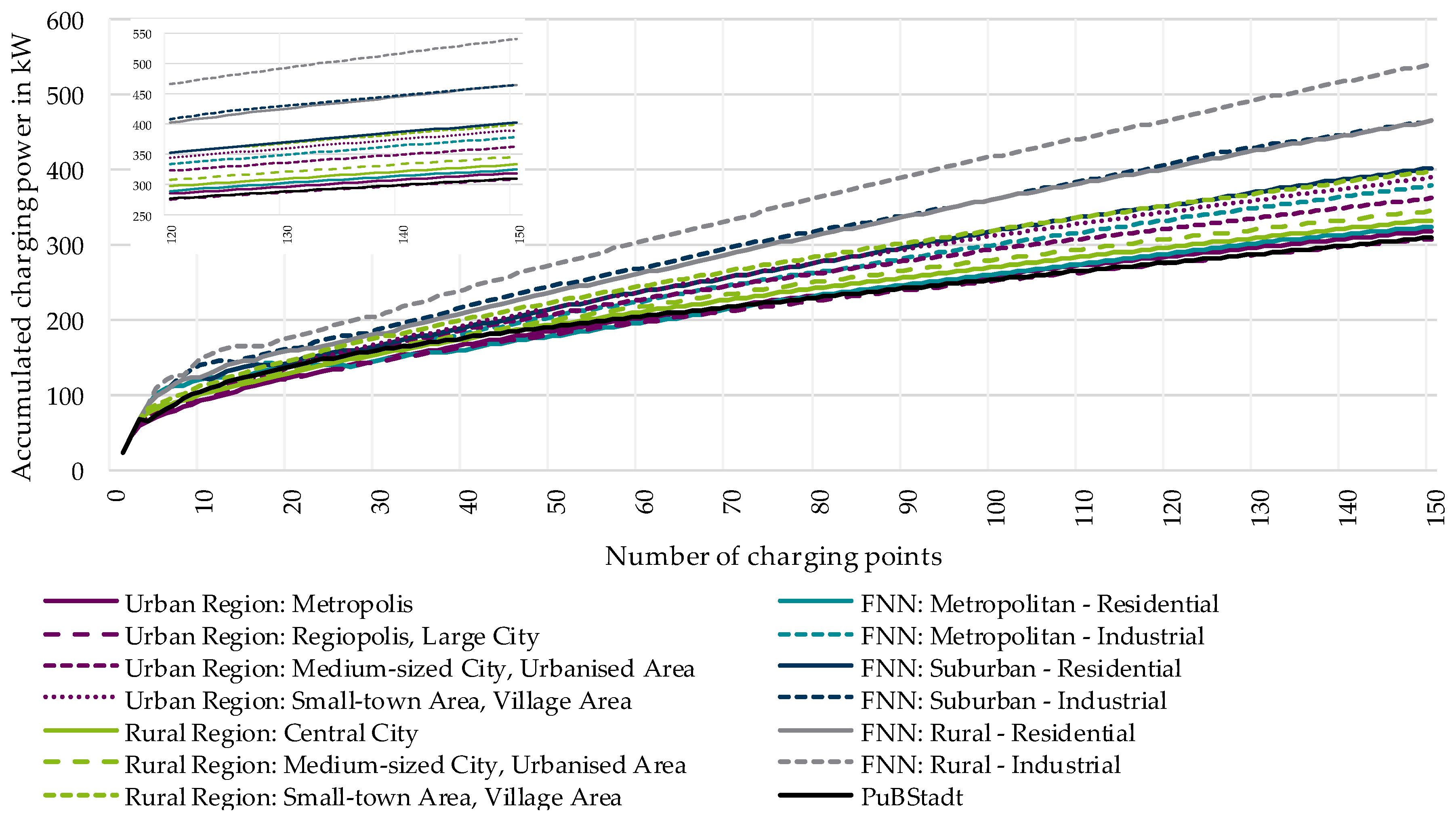
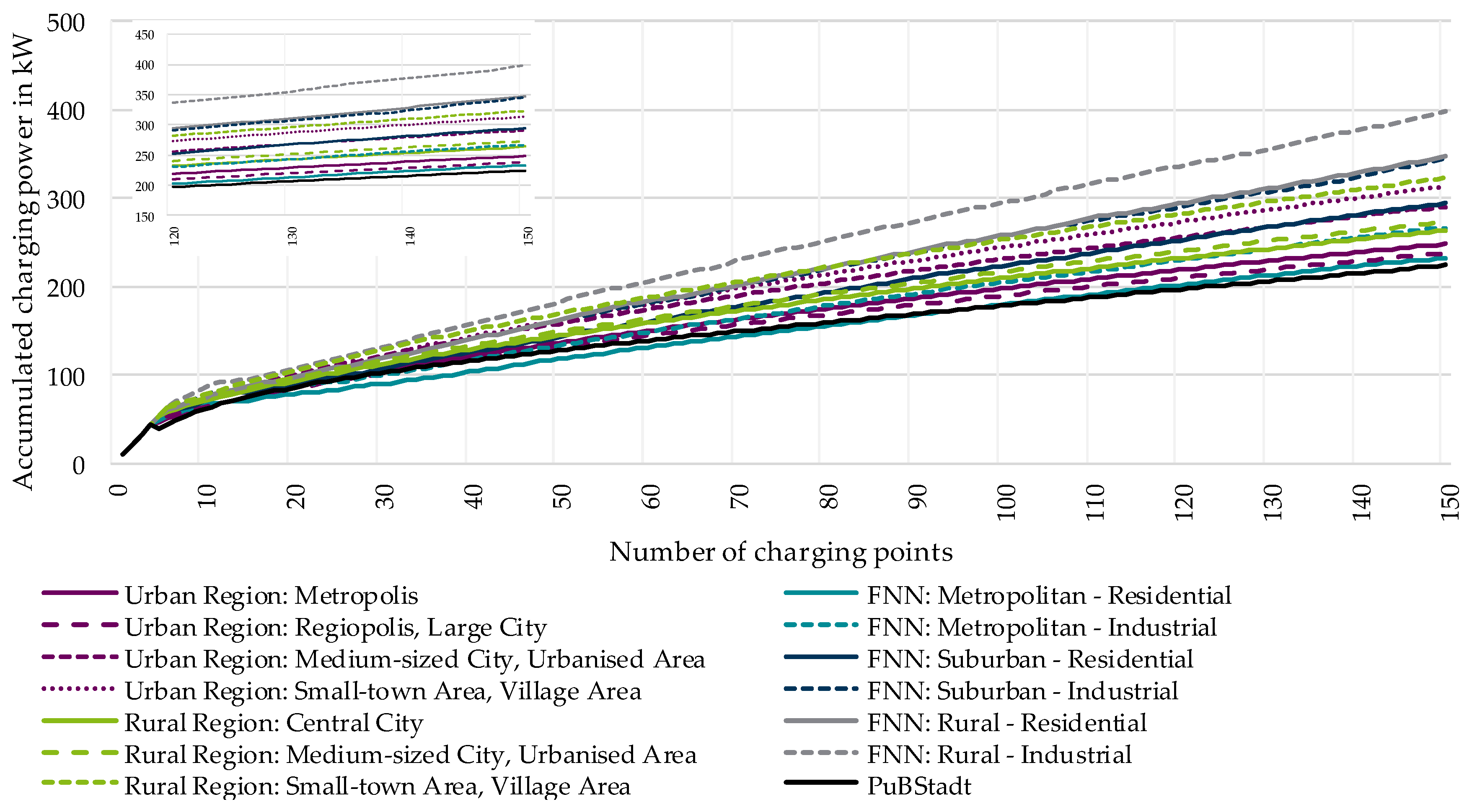
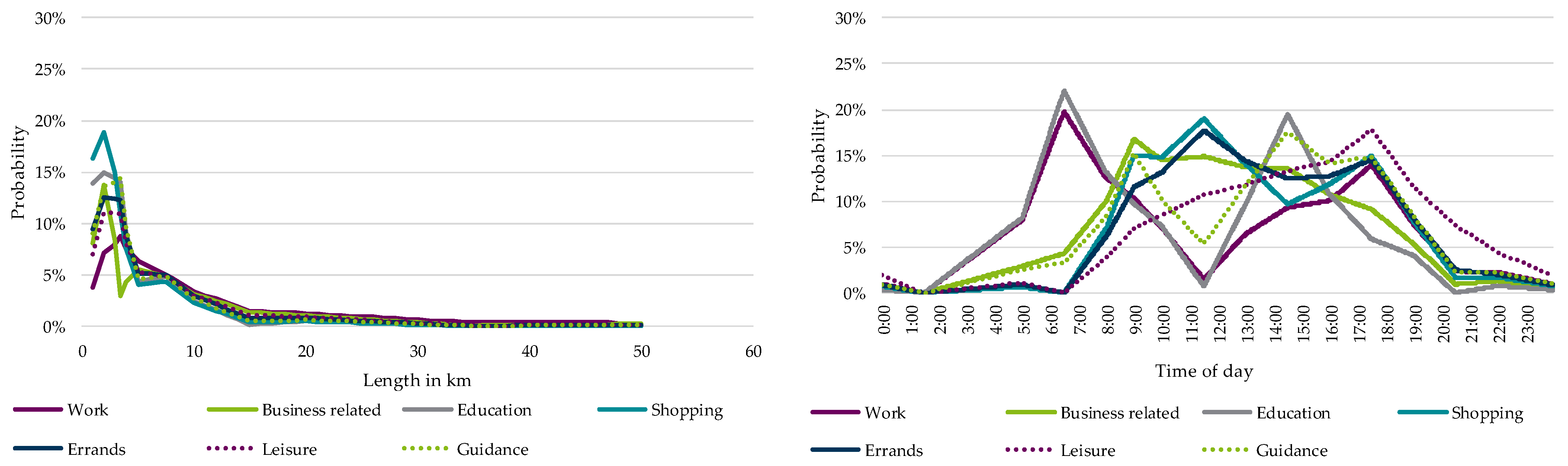
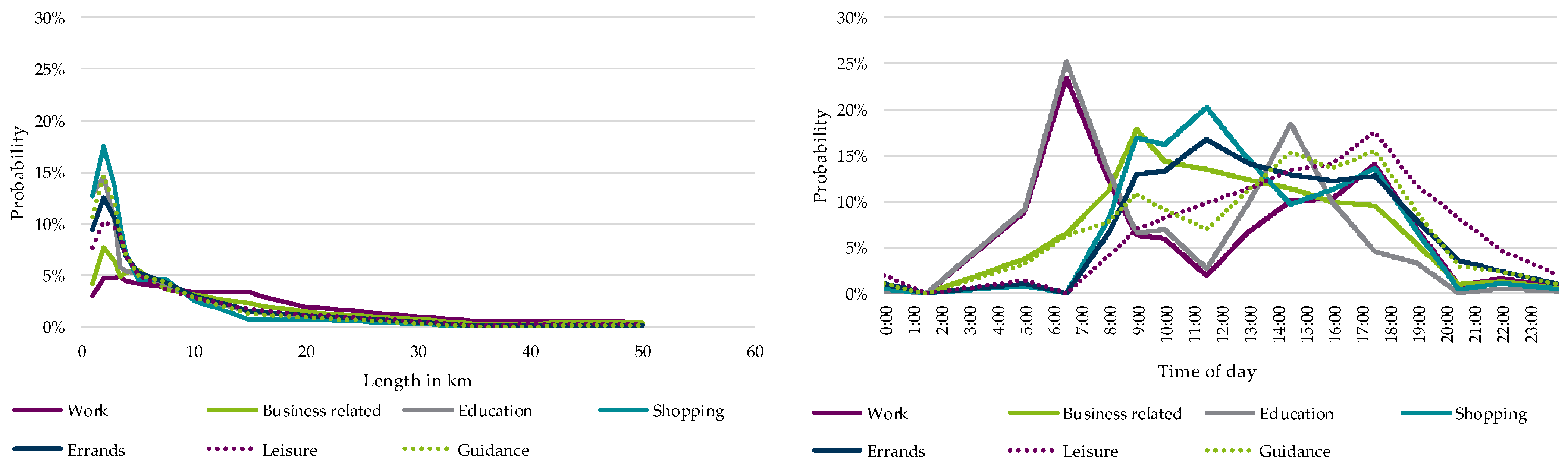
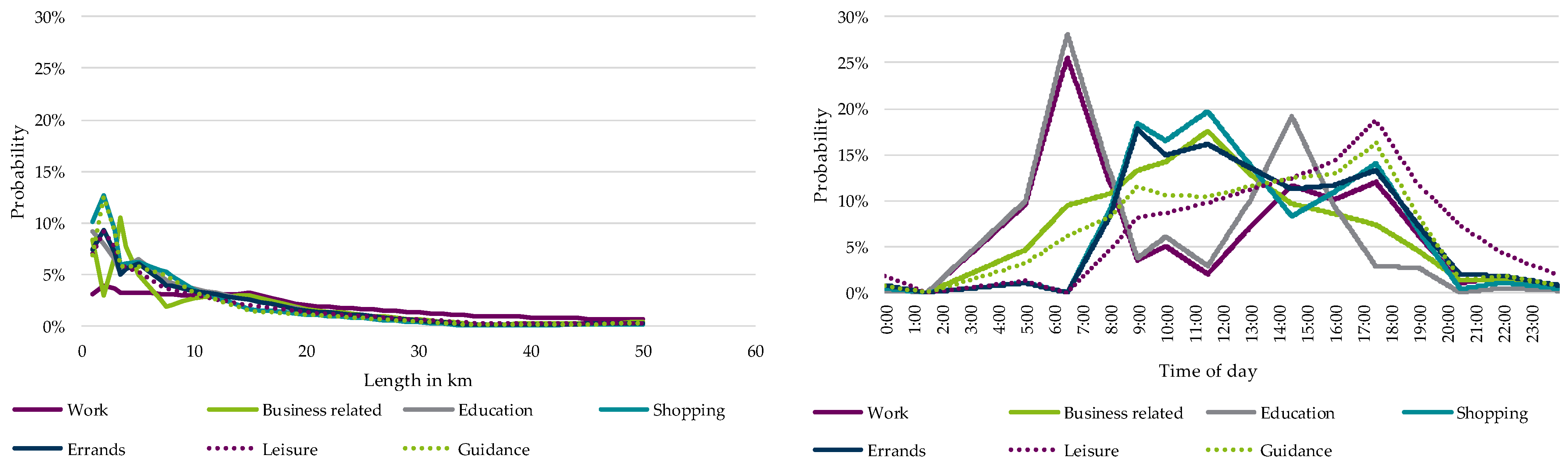
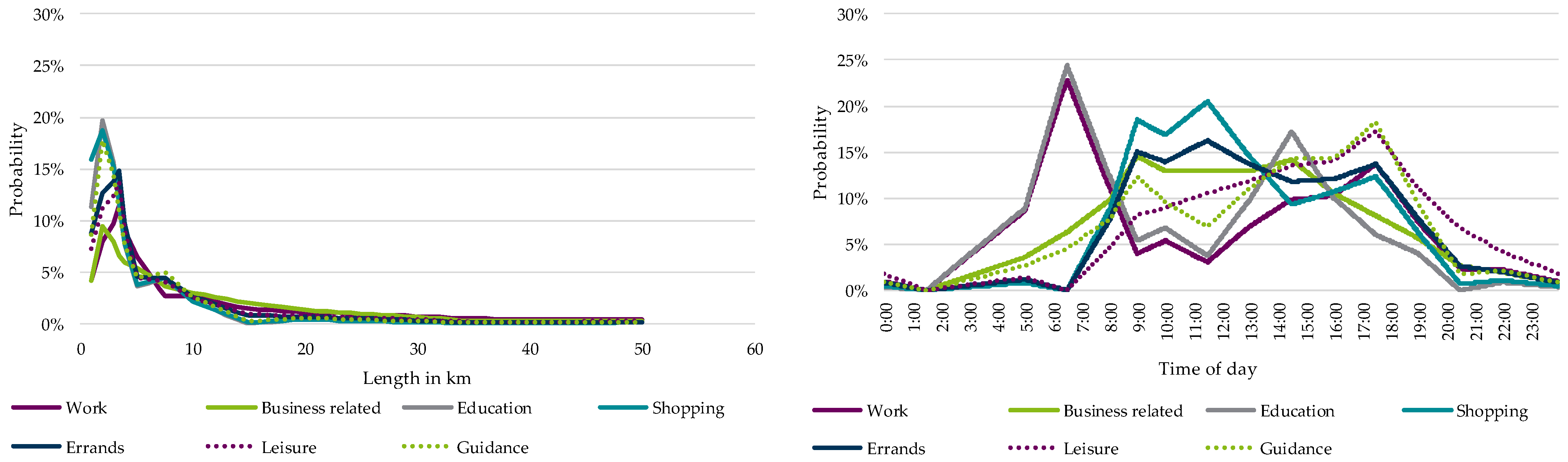
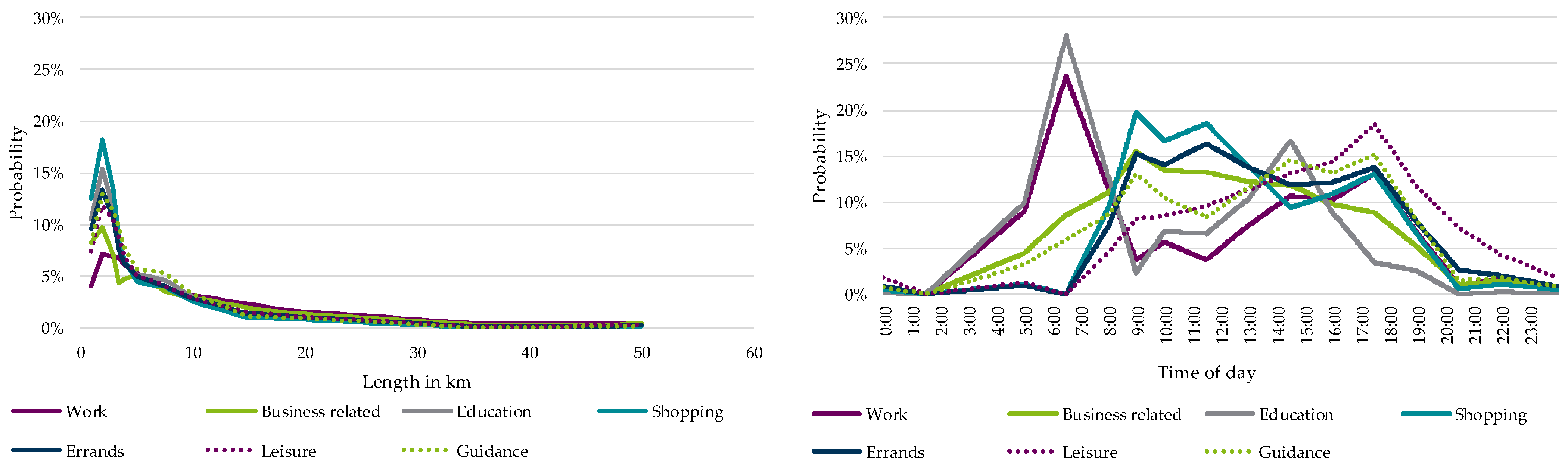
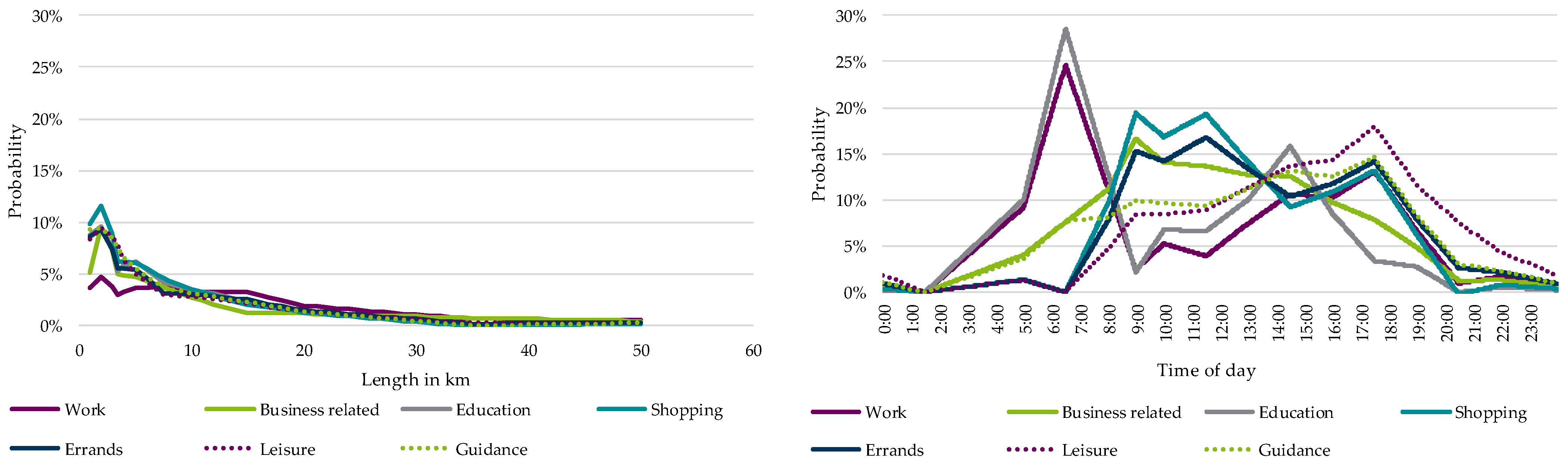
• Since the CPs are available at the destinations, the travelling distance to a CP is already included in the applied statistical driving data (Figure 3, Figure A1, Figure A2, Figure A3, Figure A4, Figure A5 and Figure A6) for the different area types. Hence, the travel distance and time of the EV(s) to a CP are modelled by generating the driving profile(s) to a certain destination.

An exemplary weekly charging profile for a charging power of 11 kW is shown in Figure 6. The result shows that with ten EVs taken into account and an assumed chaotic charging, a maximum of four EVs charge simultaneously within a week.

A further study [31] investigates the influence of a decreasing charging power after a certain state of charge (e.g., 80%). It then proves that this decrease is actually negligible in the context of strategic grid planning. Therefore, this method is not considered in this contribution.

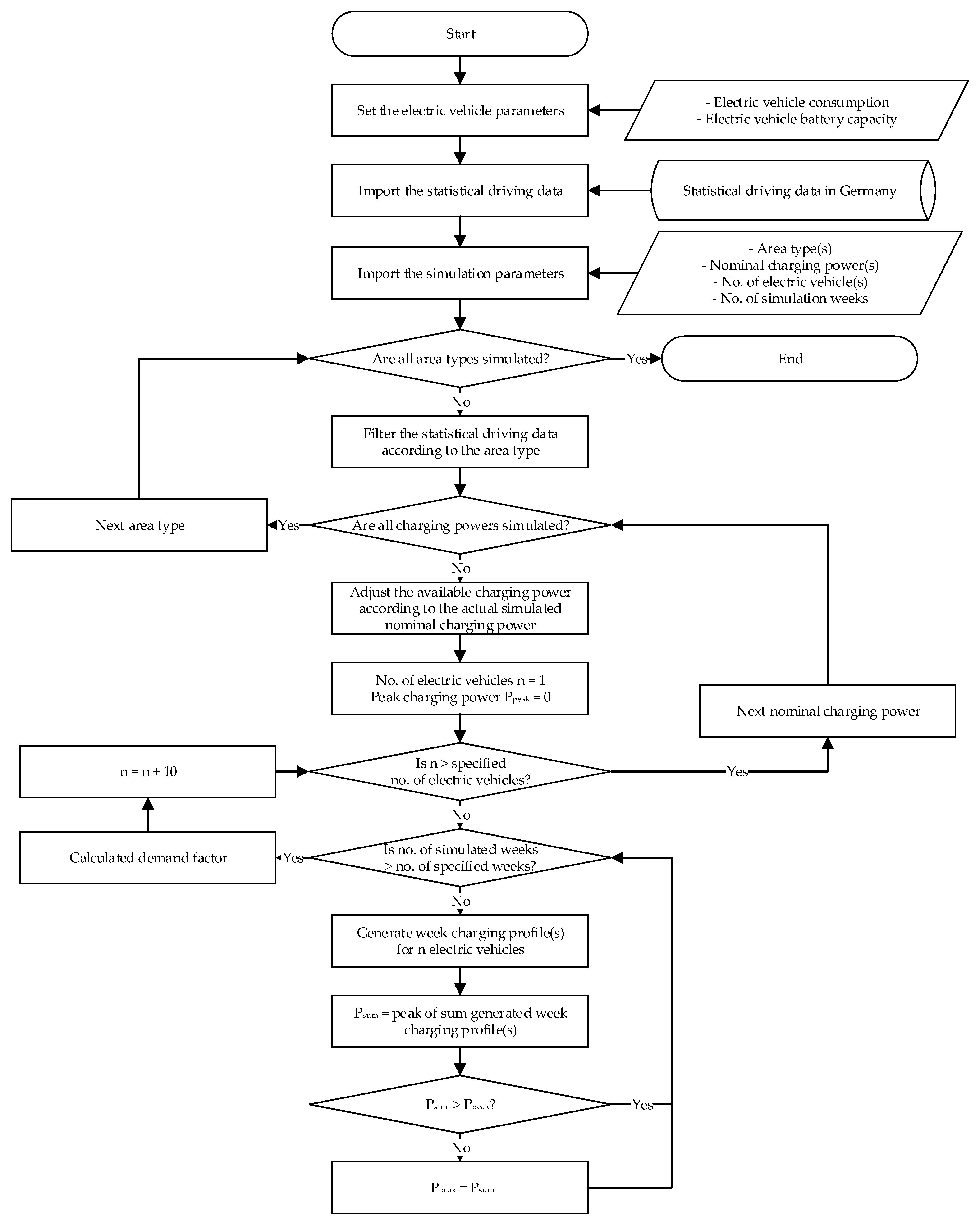
3.3. Generation of Demand Factors

To determine the DFs, charging profiles must be overlapped on a large scale in analogy to Figure 6 for a valid database, from which the maximum power values can then be calculated. In this contribution, driving profiles and the corresponding charging profiles for up to 500 EVs are generated over the span of 5200 weeks (100 years). The simulation tool iterates over four loops. The first loop generates the weekly charging profiles with the number of EVs determined in the first loop. The charging profiles are compared, and the maximum recorded power value is then taken for this specific number of EVs. By repeating the simulation 5200 times, the simulation uncertainties are eliminated, and the robustness of the results is guaranteed. The second loop increases the number of available CPs for specific charging power. This loop starts with one EV and incrementally increases the number of CPs with a step of 10 EVs until the maximum of 500 EVs. A step size of 10 EVs is used in the calculation to reduce the simulation time. The above-mentioned simulation is then repeated for the common nominal charging powers of (3.7, 11, 22, 50, 150 and 350) kW, as well as for the seven area types. In total, four nested loops are run to generate the results according to the following pseudocode:

Sub Demand_factor_tool ()

For area type = 1 to 7

For charging power = {3.7, 11, 22, 50, 150, 350}

For number of EVs = 1 to 500 with a step of 10

For simulated week = 1 to 5200

generate charging profiles for the number of EVs

overlap generated charging profiles

If maximum charging profile < charging profile then

maximum charging profile = charging profile

End if

next simulated week

calculate demand factor

Next number of EVs

Next charging power

Next area type

The (3.7, 11 and 22) kW represent private charging powers, whereas (11, 22, 50, 150 and 350) kW represent public charging powers. According to [20], 11 kW and 22 kW are so far implemented in puCPs as well as in prCPs.

The respective DF is calculated using Equation (1),

$$D{F}_{\mathrm{n},\mathrm{p}}=\frac{P_{\mathrm{n},\mathrm{p}}}{n·p}$$

(1)

where DF_n,p is the DF resulting from the cumulative charging power P_n,p for n CPs of the nominal power p [20].

Figure 7 shows an example of the results for the area type “Urban Region: Metropolis” with the aforementioned dominant charging powers. By overlapping the charging profiles per nominal power, the respective maximum value is determined for a certain number of EVs. As the number of EVs increases, the respective DF decreases following Figure 6. However, it also becomes clear in detail that the values can also briefly increase again at certain points before they then continue to decrease. This is due to the mobility data and the stochastically generated driving profiles. It only leads to the fact that the generated DF curves have to be smoothed methodically with a curve fitting to remove these anomalies [20].

The following Figure 8 shows a process diagram explaining how the simulation tool calculates the DFs. It starts by importing the general conditions mentioned in Section 3.1. It continues to import the database described in Section 2. The tool then imports the specified simulation parameters; in this case, they are the aforementioned seven area types, the charging powers (3.7, 11, 22, 50, 150 and 350) kW and the number of iterations/simulations weeks (5200 weeks). When the simulation weeks are exhausted, the DF is calculated for the specific area type, charging power and number of EVs. The simulation tool proceeds to the next number of EVs with a step size of ten. When the total number of EVs is simulated, the simulation tool continues with the next charging power and eventually the next area type until a DF for each combination of the simulation parameters is calculated.

For curve smoothing, the curve-fitting toolbox from the software MATLAB [32] is used and is exemplified in Figure 9. Two curve fitting iterations are run consequently. The first iteration is run to the DF values generated by the simulation tool to smoothen out the rigid curves shown in Figure 7. It also interpolates the DF values for the numbers of EVs per 1 EV step based on the generated 10 EV step. The second curve fitting iteration is performed to calculate the DF for the charging powers between 3.7 kW and 350 kW per 1 kW step. Since the generated DF values are for only six charging powers, the DF values for all the charging powers within these are deduced for each number of CPs. The main idea for the conducted curve fitting depends on the fact that the DF values for the charging powers between each of the charging powers can be interpolated depending on the existing values. For instance, the DFs for the charging powers between 3.7 kW and 11 kW (e.g., 4 kW, 5 kW, 6 kW up to 10 kW) must lie between the DF values of 3.7 kW and 11 kW. By interpolating the values using a curve-fitting algorithm, the DF values for all power values between 3.7 kW and 350 kW can be determined as shown in Figure 9. The detailed method is explained in [20].

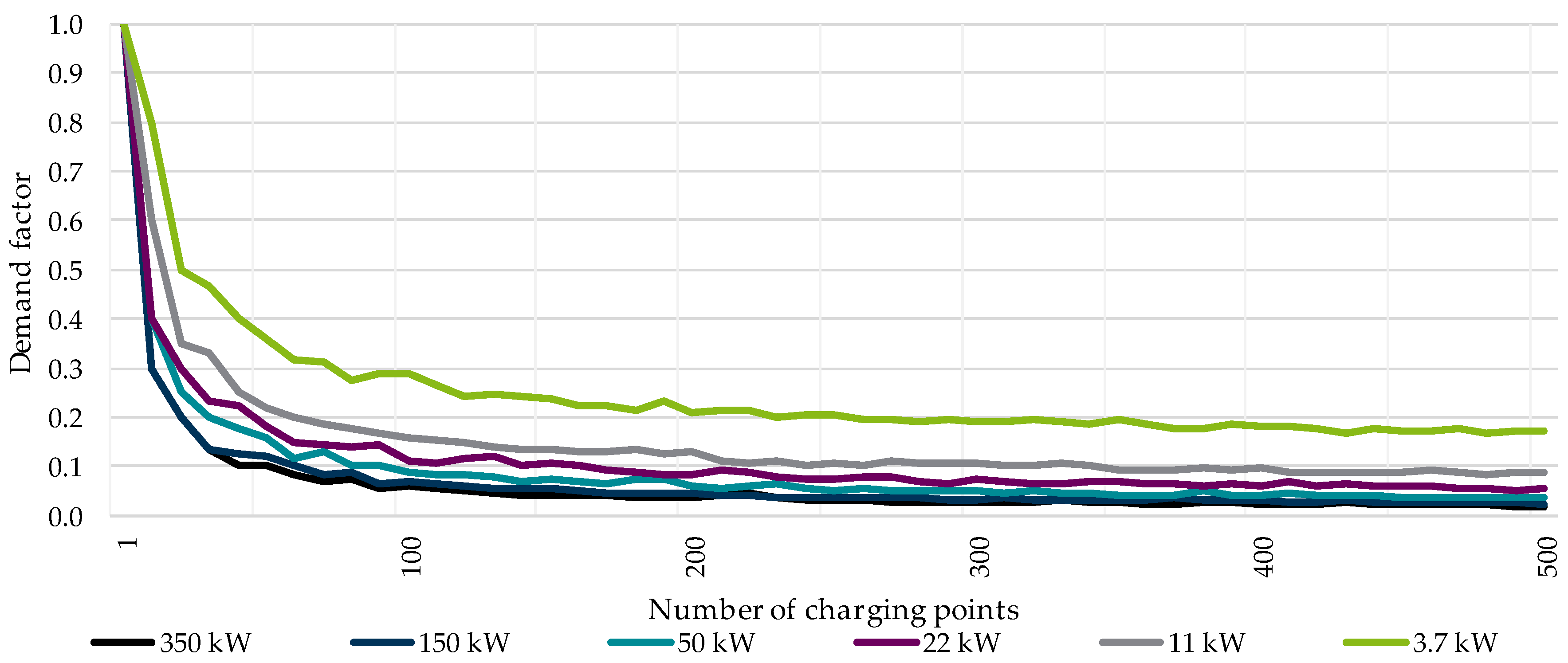
4. Results of the Simulation

Based on the methodology in Section 3, the DF values are generated as the results of the simulation. The goal here is to provide distribution system operators with the required values for performing strategic grid planning by displaying the DF curves for the seven area types and for the six main nominal charging powers. In addition, the DF values are provided in a tabular form in Appendix B. Although the figures may seem significantly alike, the minimal differences between the DF values can result in considerable differences in the resulting accumulated charging power.

Figure 10 shows an example result from the DF developed according to the database and the method explained in Section 2 and Section 3, respectively. The nominal charging powers are highlighted in colour. The intermediate charging powers in grey are required depending on the method used to calculate the accumulated resulting charging power for strategic grid planning according to [25]. The method in [25] determines the accumulated resulting charging power based on a calculated effective mean charging power which—in most cases—does not correspond to one of the nominal charging powers.

In addition, Figure 10 shows that the DFs decrease rapidly for an increasing number of CPs but eventually start to saturate around 300 CPs. According to [33], the DF values reach a nearly constant value starting from around 500 CPs. Hence, the presented DFs stay valid and can be applied to more than 500 CPs.

For better visibility, the charging powers in 1 kW steps between 50 kW and 150 kW and between 150 kW and 350 kW are hidden. However, they are already calculated. In the following two sections, the calculated DFs are compared in separate analyses.

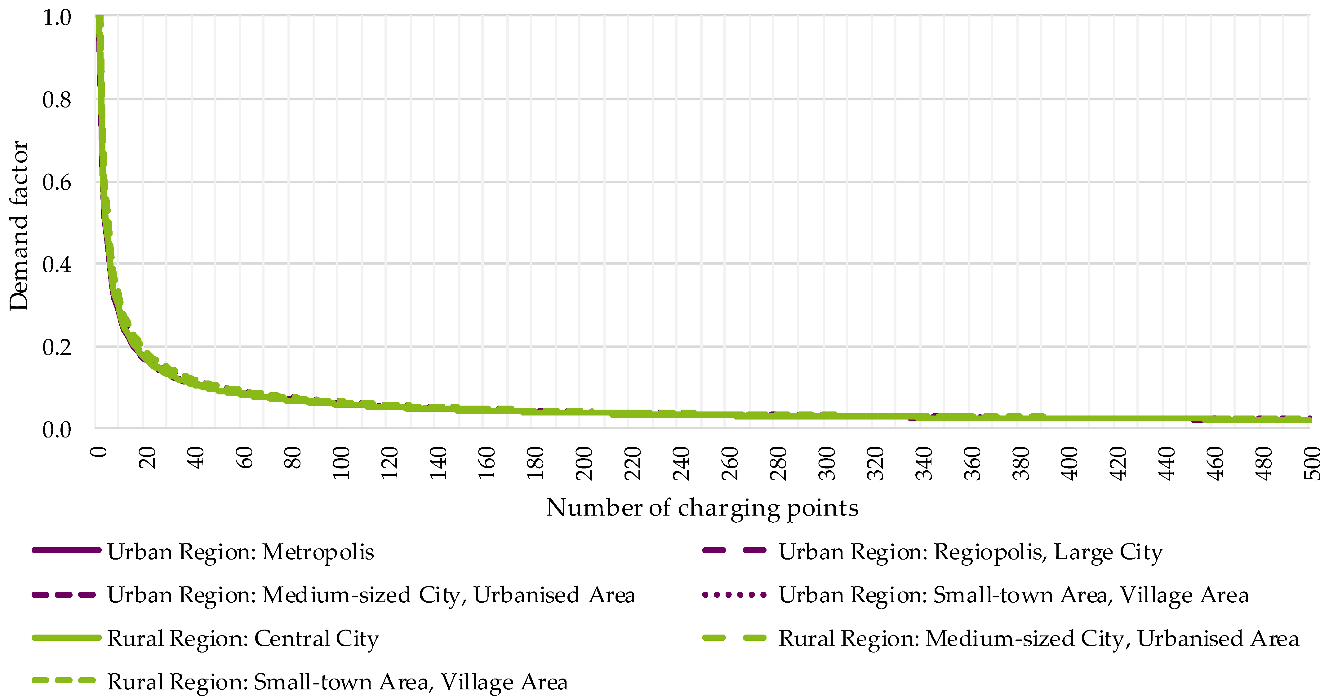
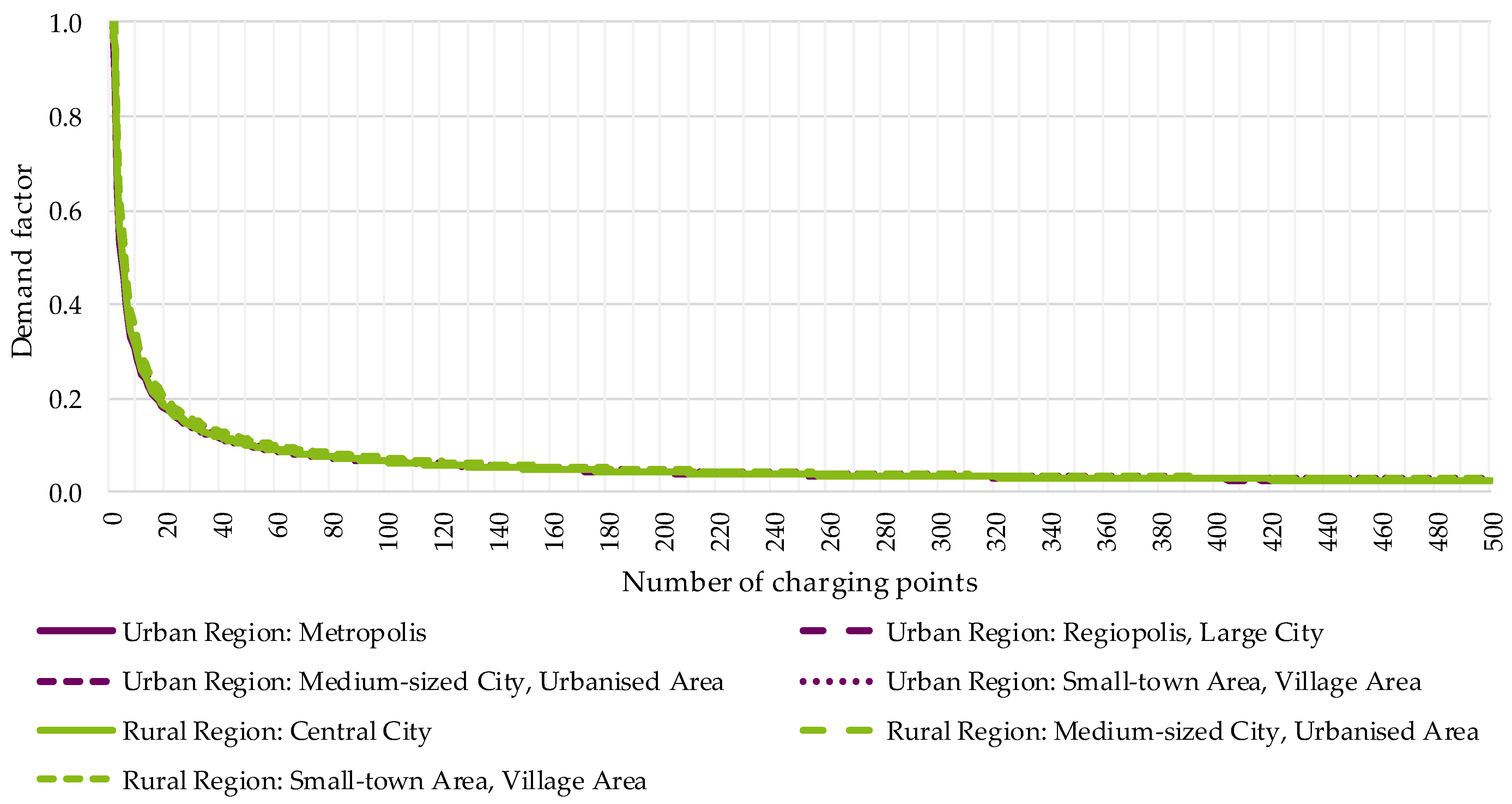
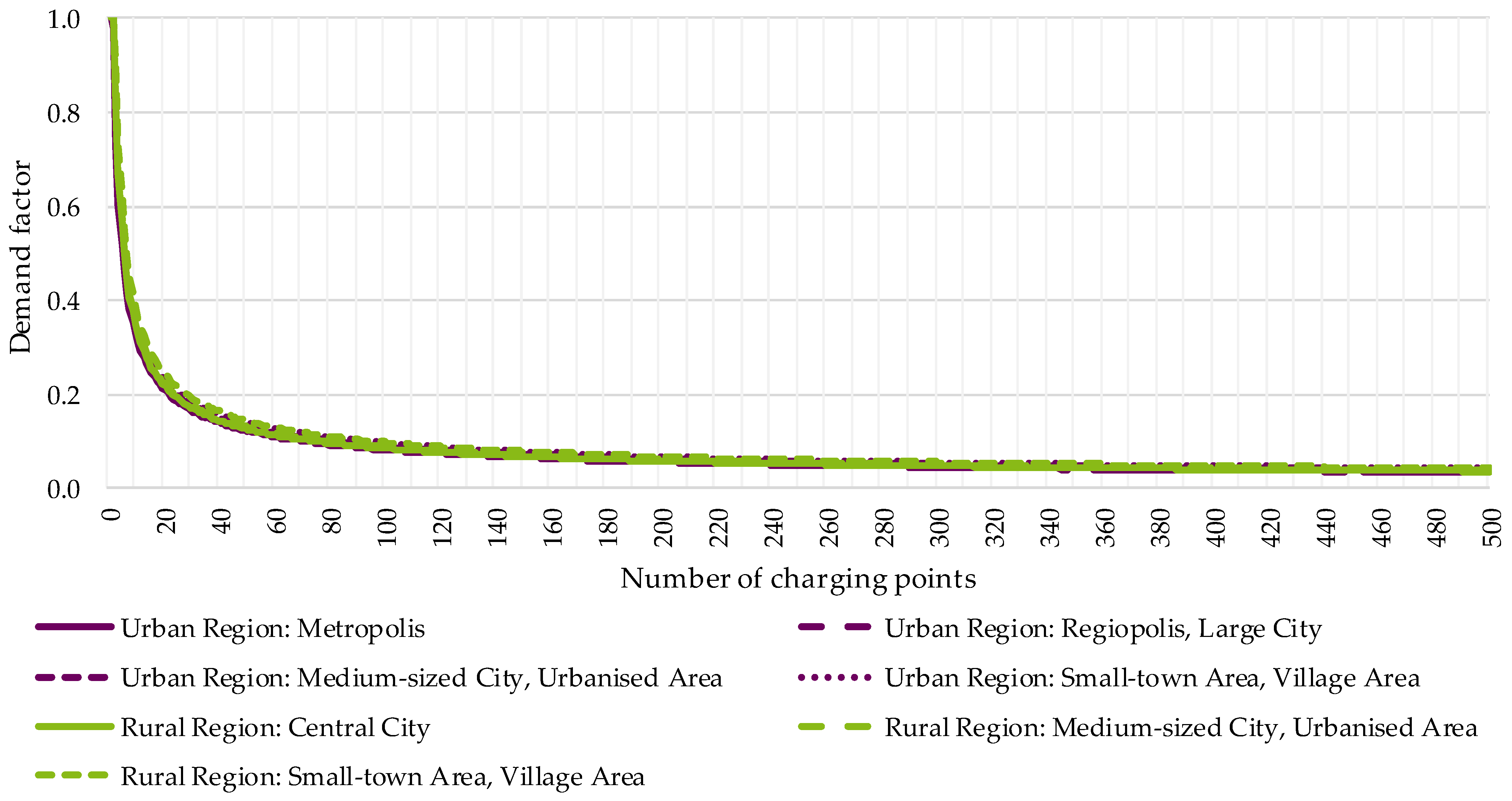
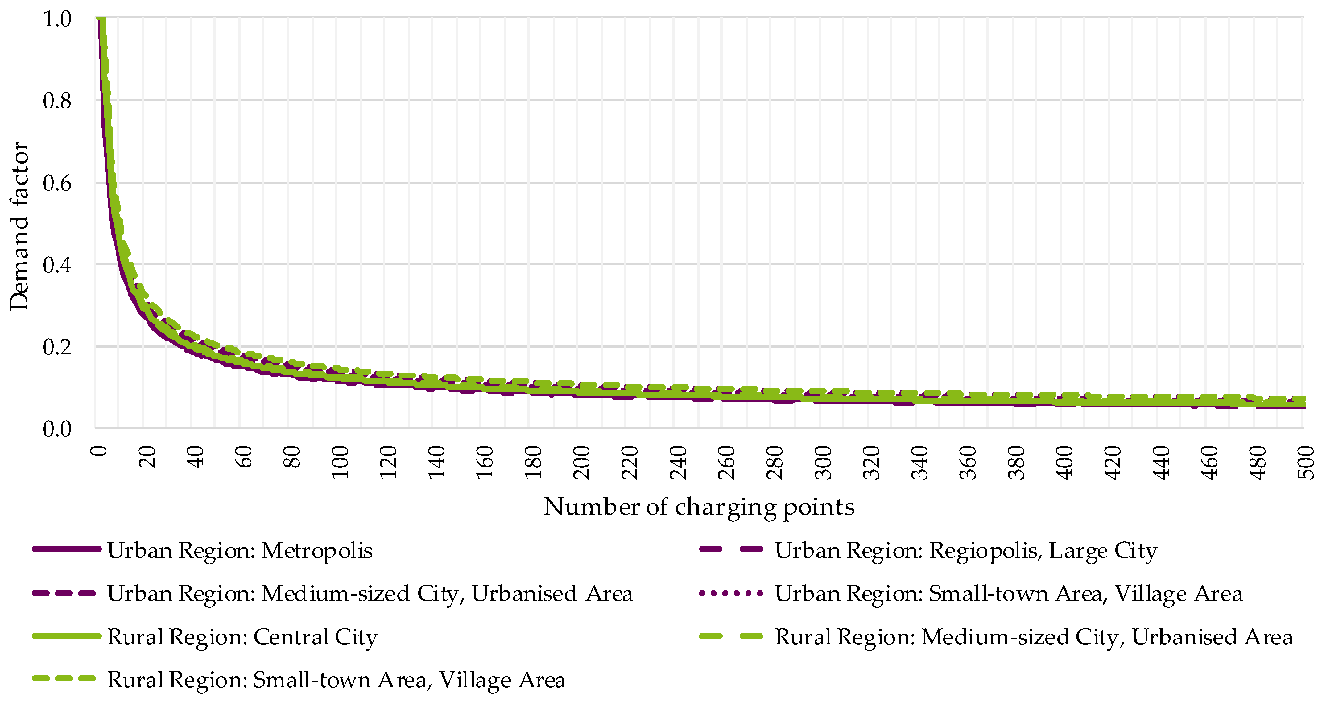
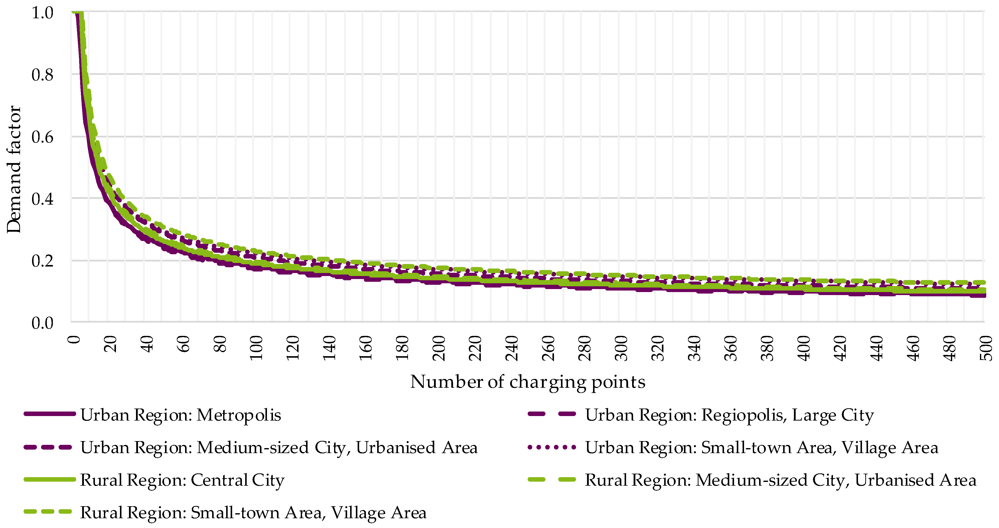
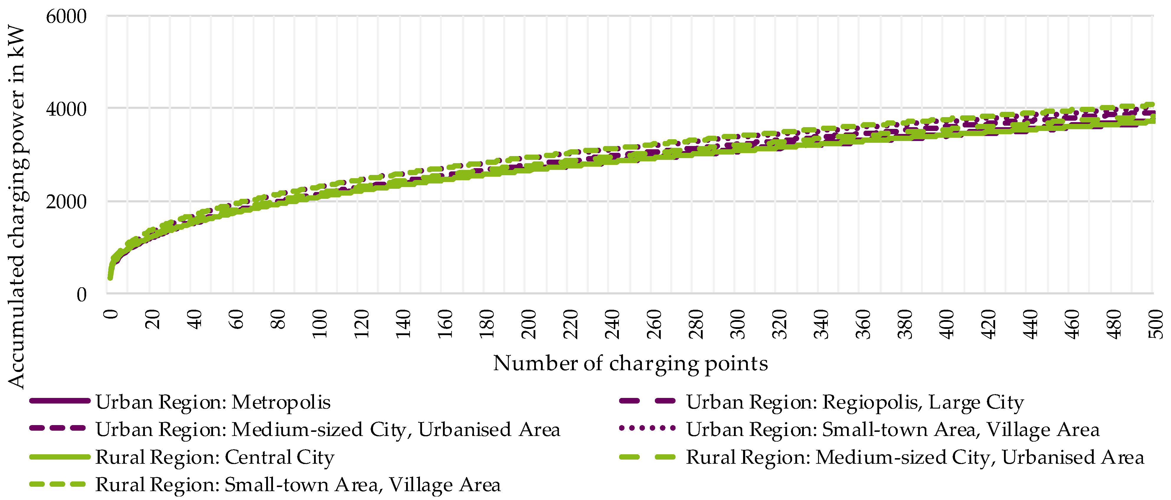
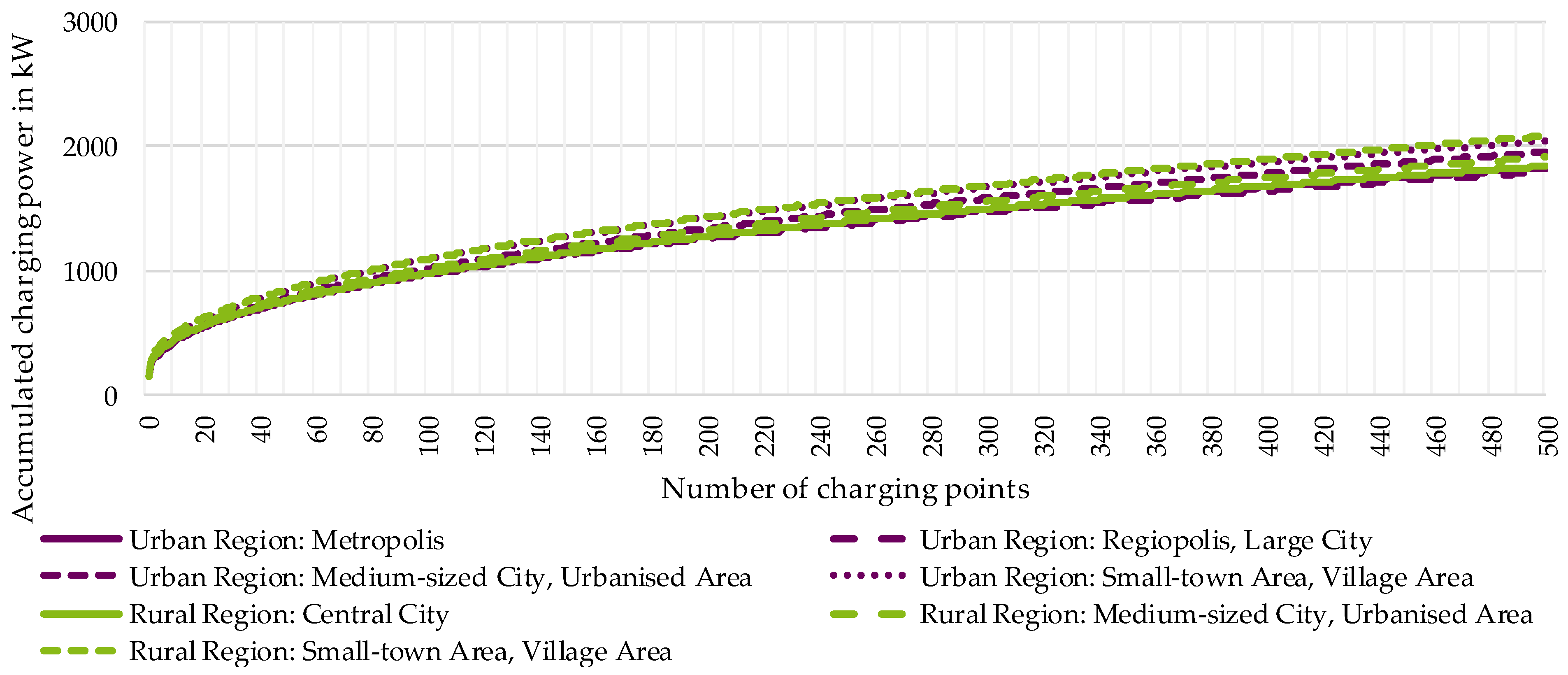
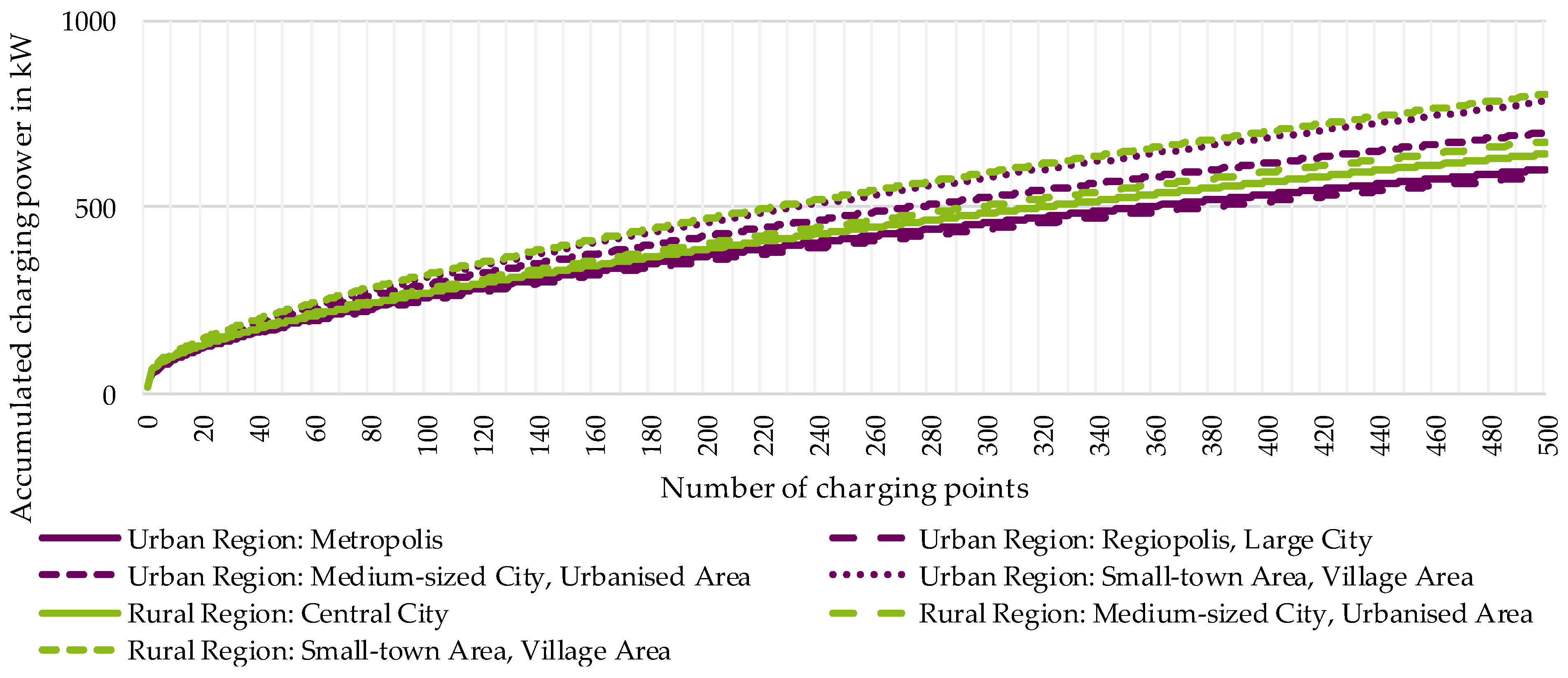
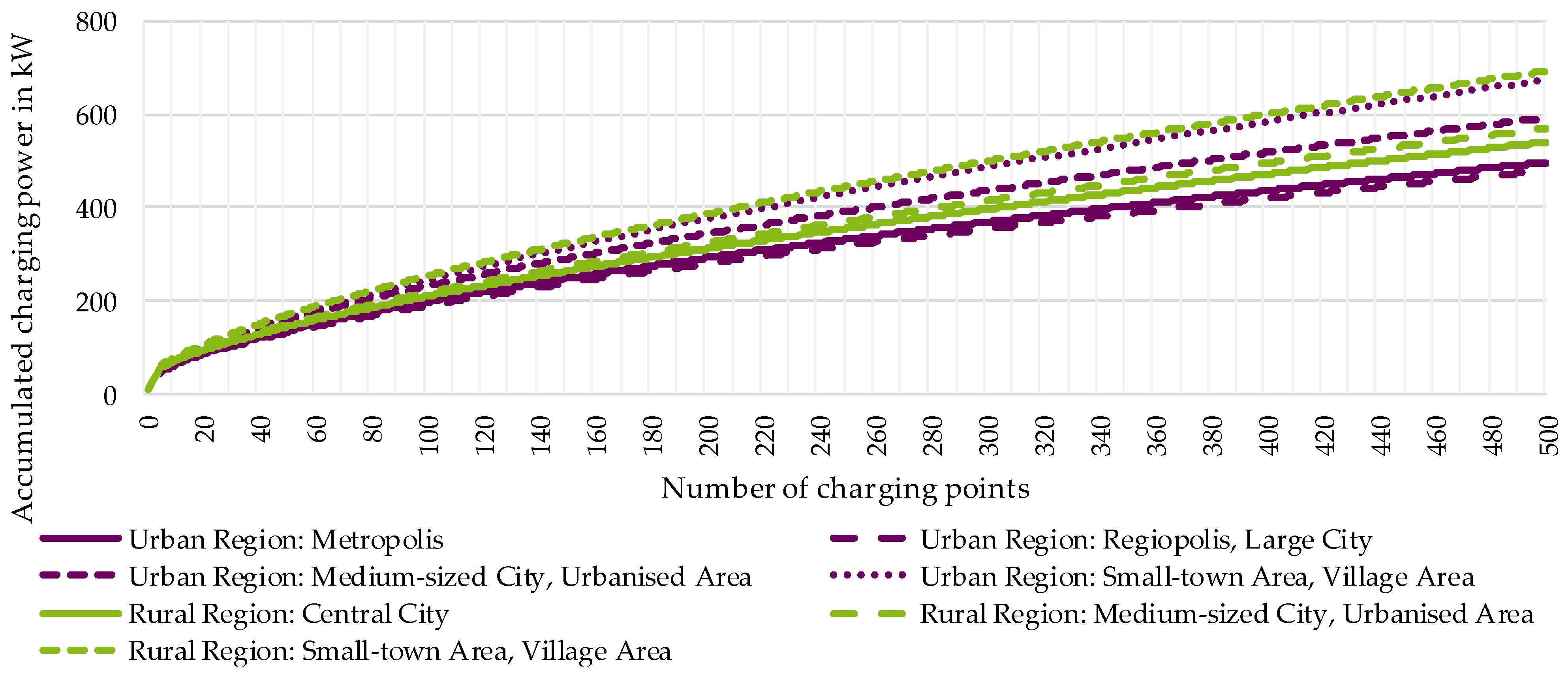
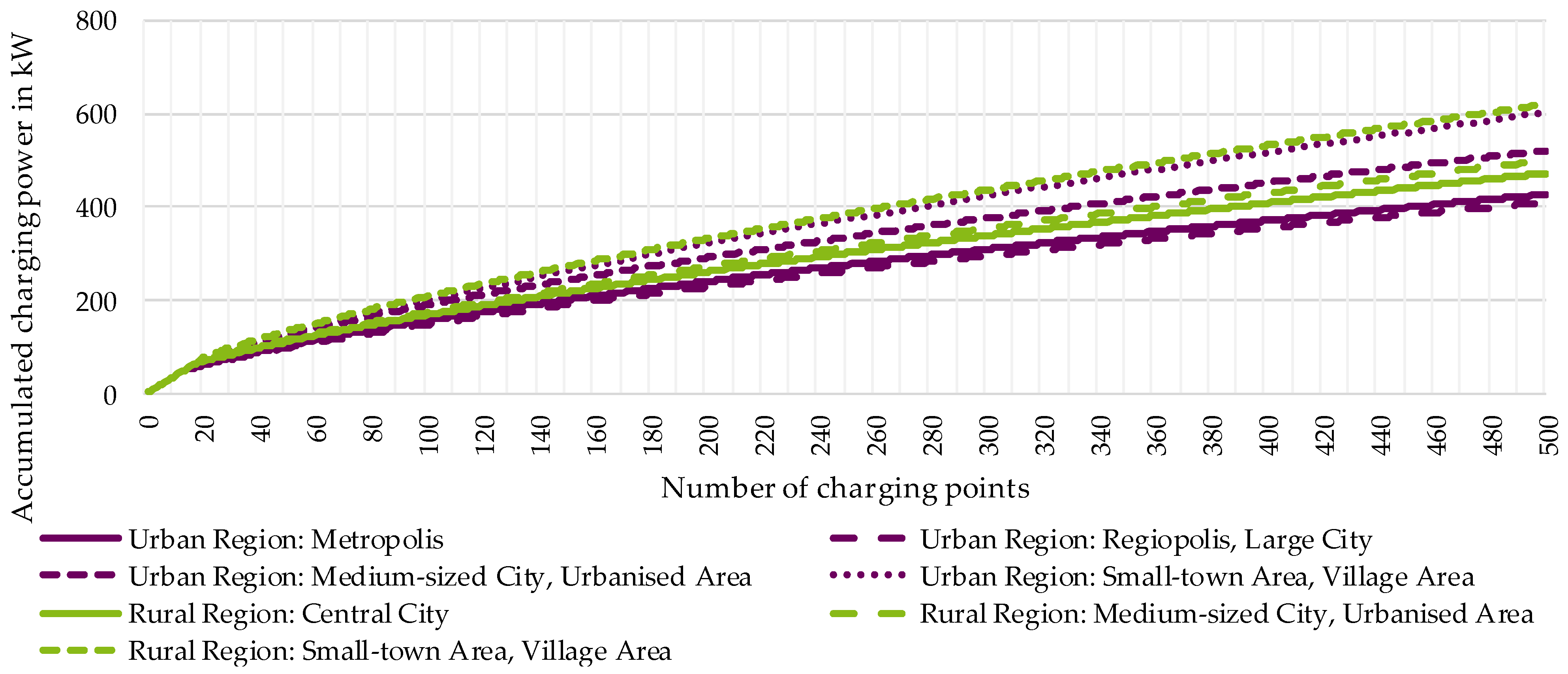
4.1. Demand Factors According to the Area Types

For the six main nominal charging powers, the DFs can be assumed according to Figure 11 for the area type “Urban Region: Metropolis”, Figure 12 for the area type “Urban Region: Regiopolis, Large City”, Figure 13 for the area type “Urban Region: Medium-sized City, Urbanized Area”, Figure 14 for the area type “Urban Region: Small-town Area, Village Area”, Figure 15 for the area type “Rural Region: Central City”, Figure 16 for the area type “Rural Region: Medium-sized City, Urbanized Area” and Figure 17 for the area type “Rural Region: Small-town Area, Village Area”.

The results show that the DFs strongly decrease with increasing charging power. The greatest difference can be seen graphically in the following figures (and tabularly in Appendix B in the

Table A1. Demand factors for the area type “Urban Region: Metropolis” and six charging powers.

Charging Points	350 kW	150 kW	50 kW	22 kW	11 kW	3.7 kW
5	0.44	0.46	0.52	0.64	0.85	1.00
10	0.27	0.28	0.33	0.41	0.57	1.00
50	0.09	0.10	0.12	0.17	0.25	0.56
100	0.06	0.06	0.08	0.12	0.18	0.43
500	0.02	0.02	0.03	0.05	0.09	0.23

,

Table A2. Demand factors for the area type “Urban Region: Regiopolis, Large City” and six charging powers.

Charging Points	350 kW	150 kW	50 kW	22 kW	11 kW	3.7 kW
5	0.44	0.46	0.54	0.68	0.93	1.00
10	0.27	0.29	0.33	0.42	0.58	1.00
50	0.09	0.10	0.12	0.16	0.24	0.54
100	0.06	0.06	0.08	0.11	0.17	0.40
500	0.02	0.02	0.03	0.05	0.09	0.22

,

Table A3. Demand factors for the area type “Urban Region: Medium-sized City, Urbanized Area” and six charging powers.

Charging Points	350 kW	150 kW	50 kW	22 kW	11 kW	3.7 kW
5	0.45	0.48	0.56	0.71	0.98	1.00
10	0.28	0.29	0.35	0.46	0.65	1.00
50	0.10	0.10	0.13	0.19	0.29	0.68
100	0.06	0.07	0.09	0.13	0.21	0.51
500	0.02	0.03	0.04	0.06	0.11	0.28

,

Table A4. Demand factors for the area type “Urban Region: Small-town Area, Village Area” and six charging powers.

Charging Points	350 kW	150 kW	50 kW	22 kW	11 kW	3.7 kW
5	0.46	0.48	0.56	0.72	0.99	1.00
10	0.29	0.31	0.36	0.46	0.65	1.00
50	0.10	0.11	0.14	0.20	0.29	0.69
100	0.07	0.07	0.10	0.14	0.22	0.54
500	0.02	0.03	0.04	0.07	0.12	0.33

,

Table A5. Demand factors for the area type “Rural Region: Central City” and six charging powers.

Charging Points	350 kW	150 kW	50 kW	22 kW	11 kW	3.7 kW
5	0.46	0.48	0.57	0.73	1.00	1.00
10	0.28	0.30	0.35	0.45	0.64	1.00
50	0.09	0.10	0.13	0.18	0.26	0.61
100	0.06	0.07	0.08	0.12	0.19	0.46
500	0.02	0.02	0.04	0.06	0.10	0.26

,

Table A6. Demand factors for the area type “Rural Region: Medium-sized City, Urbanized Area” and six charging powers.

Charging Points	350 kW	150 kW	50 kW	22 kW	11 kW	3.7 kW
5	0.45	0.48	0.57	0.76	1.00	1.00
10	0.28	0.30	0.36	0.47	0.67	1.00
50	0.10	0.10	0.13	0.18	0.27	0.63
100	0.06	0.07	0.09	0.13	0.20	0.47
500	0.02	0.03	0.04	0.06	0.10	0.27

and

Table A7. Demand factors for the area type “Rural Region: Small-town Area, Village Area” and six charging powers.

Charging Points	350 kW	150 kW	50 kW	22 kW	11 kW	3.7 kW
5	0.51	0.54	0.63	0.79	1.00	1.00
10	0.31	0.33	0.39	0.50	0.70	1.00
50	0.10	0.11	0.14	0.20	0.31	0.73
100	0.07	0.07	0.10	0.15	0.23	0.56
500	0.02	0.03	0.04	0.07	0.13	0.33

) in the DF values for the charging powers between 3.7 kW and 22 kW. In contrast, no clear graphical distinction of the DFs can be detected between the area types for the charging powers 50 kW, 150 kW and 350 kW. Moreover, the DF values for the charging powers 150 kW and 350 kW are nearly equal in all area types. Thus, it can be deduced that the expected fast CPs (CPs with a power equal to or greater than 150 kW) have a nearly equal DF independent of the actual charging power and area type.

By carefully examining Figure 11, Figure 12, Figure 13, Figure 14, Figure 15, Figure 16 and Figure 17, a difference in DF values can be identified between the seven area types, even though the simulation tool parameters do not change among them. These differences result from the varying driving profiles for the seven area types. The differences in the driving profiles are highlighted in Figure 3 and Figure A1, Figure A2, Figure A3, Figure A4, Figure A5 and Figure A6, which are presented in Appendix A.

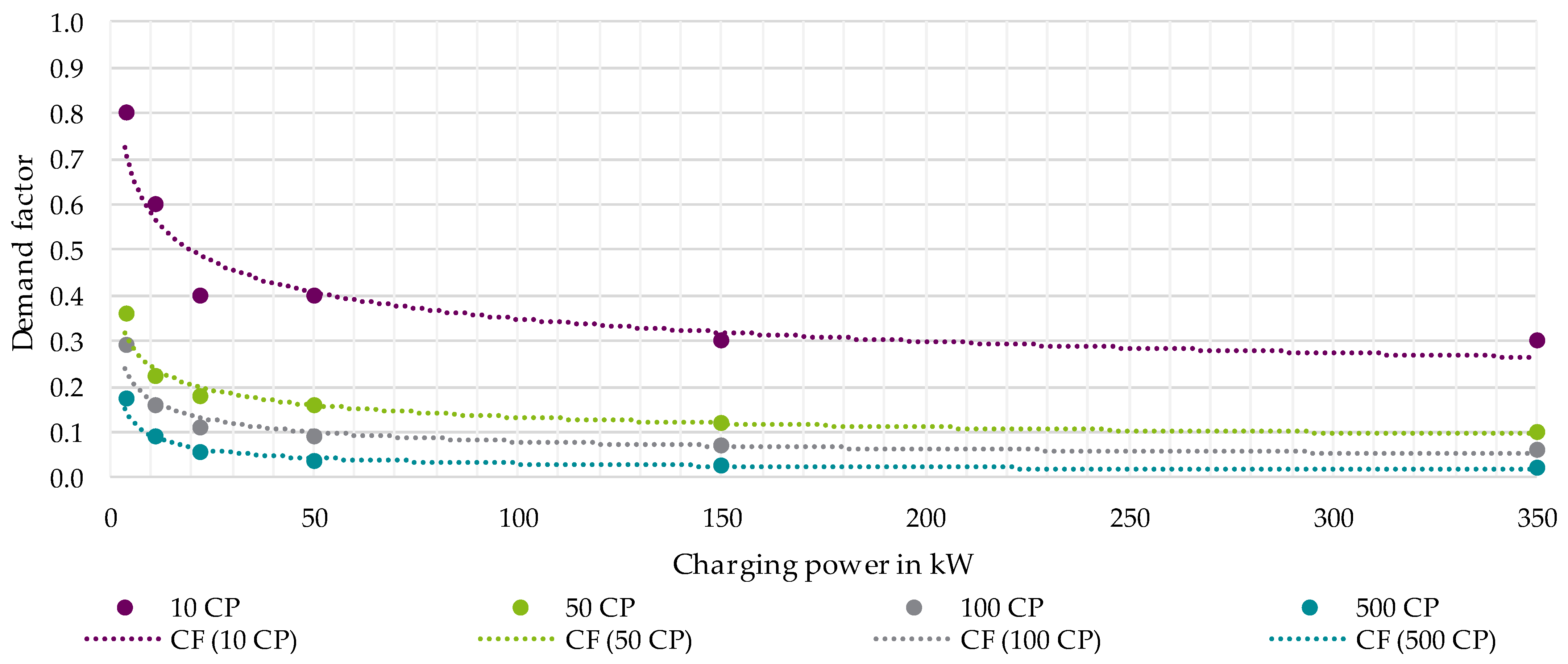
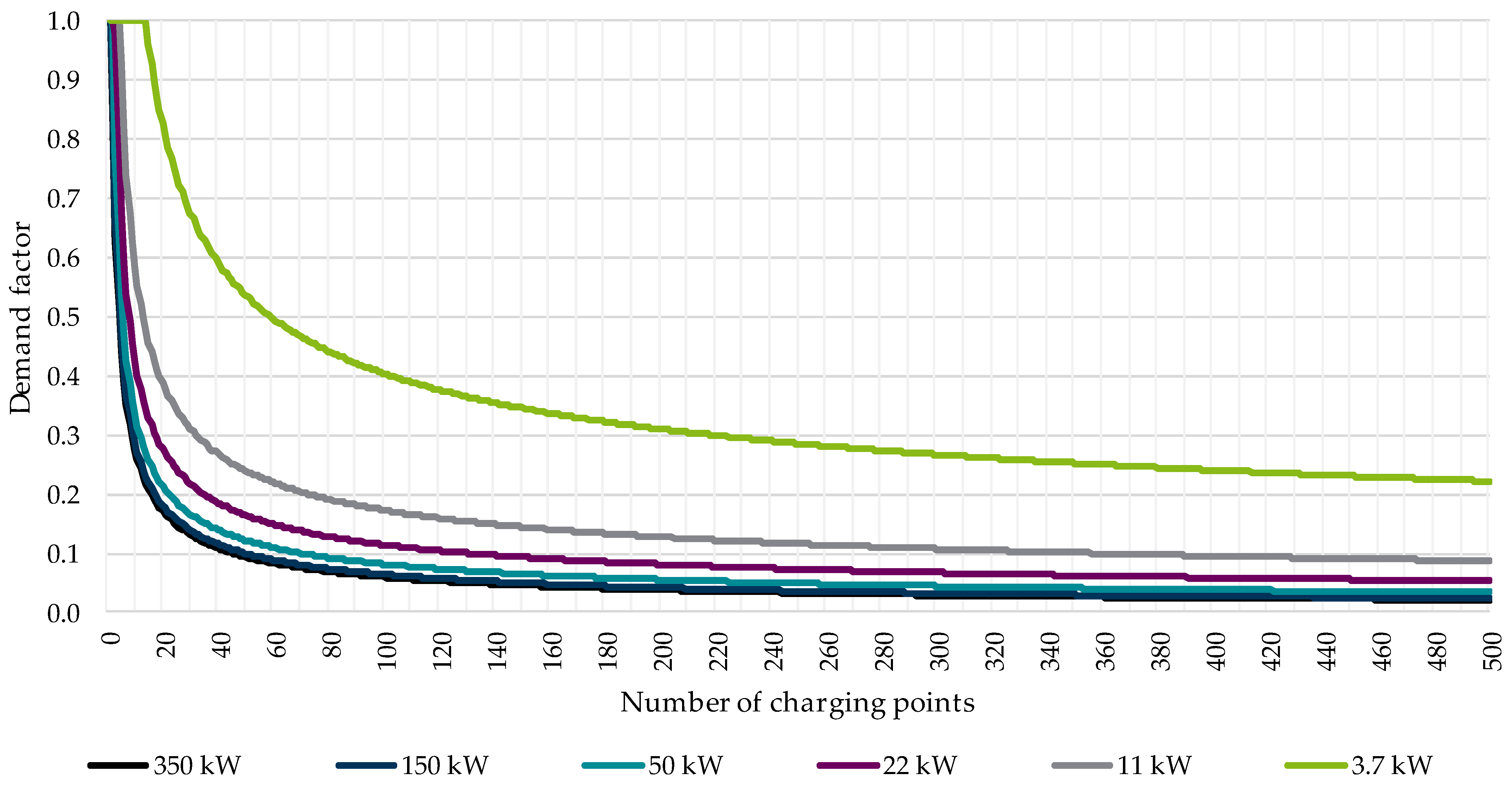
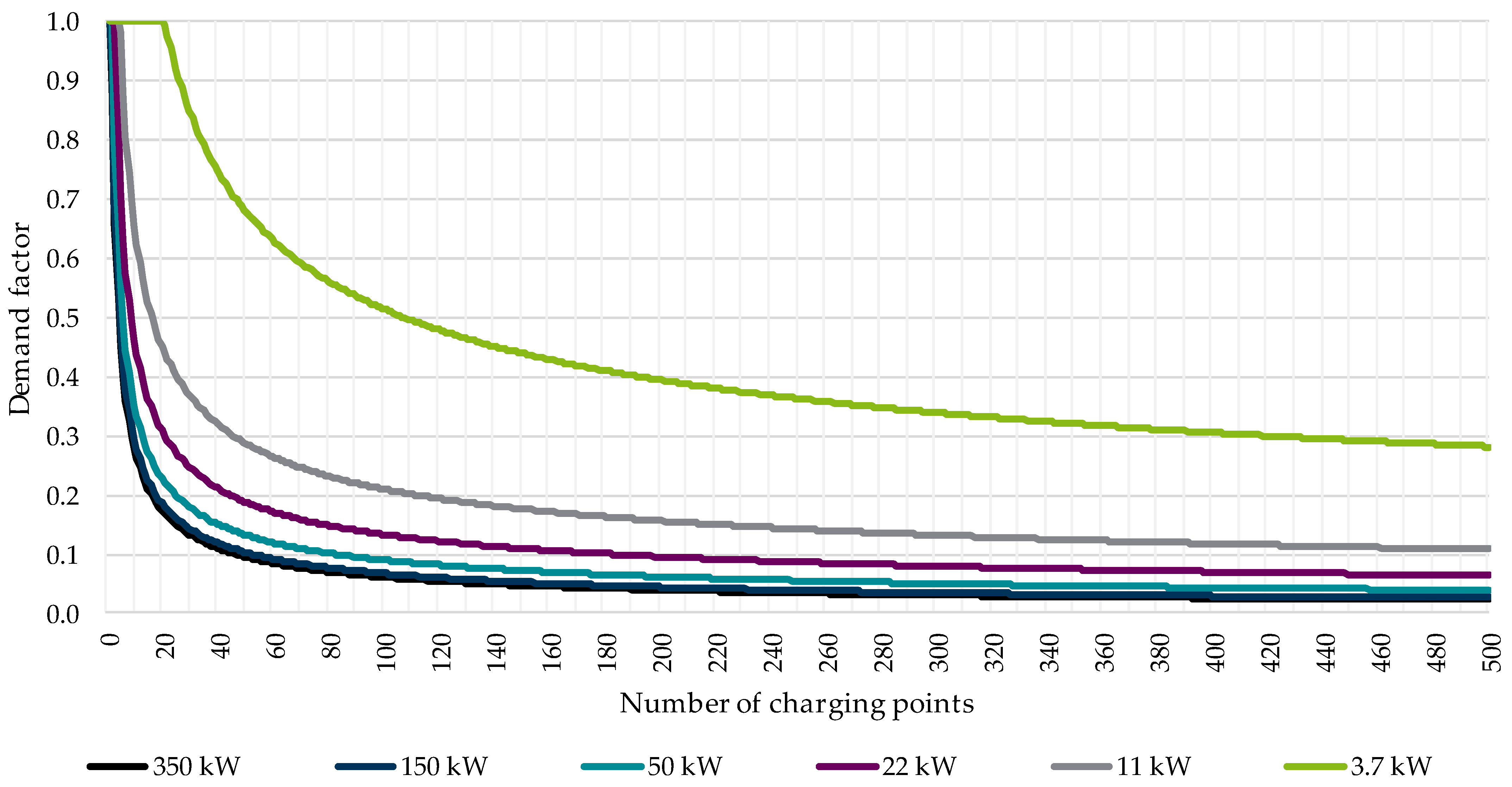
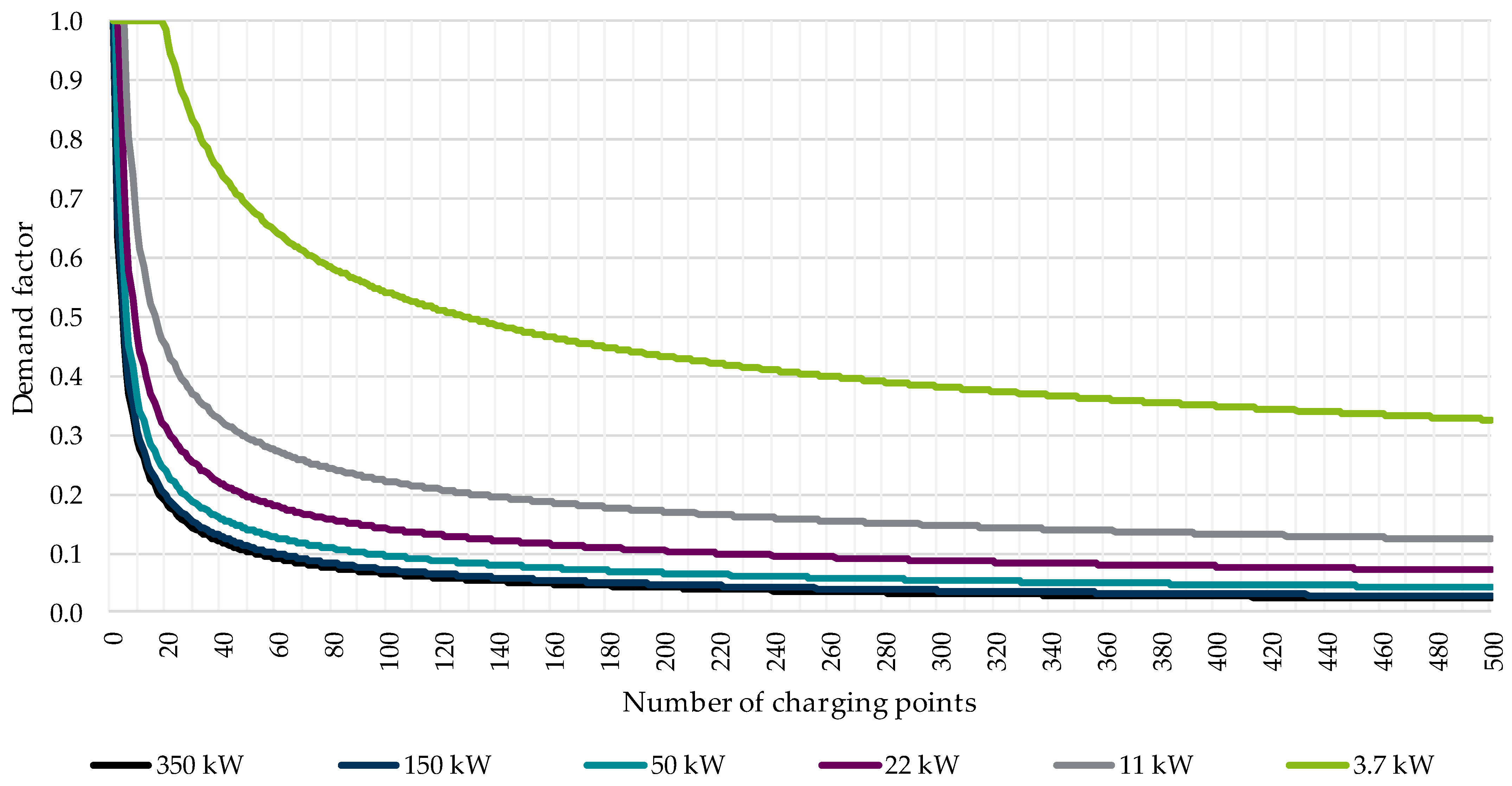
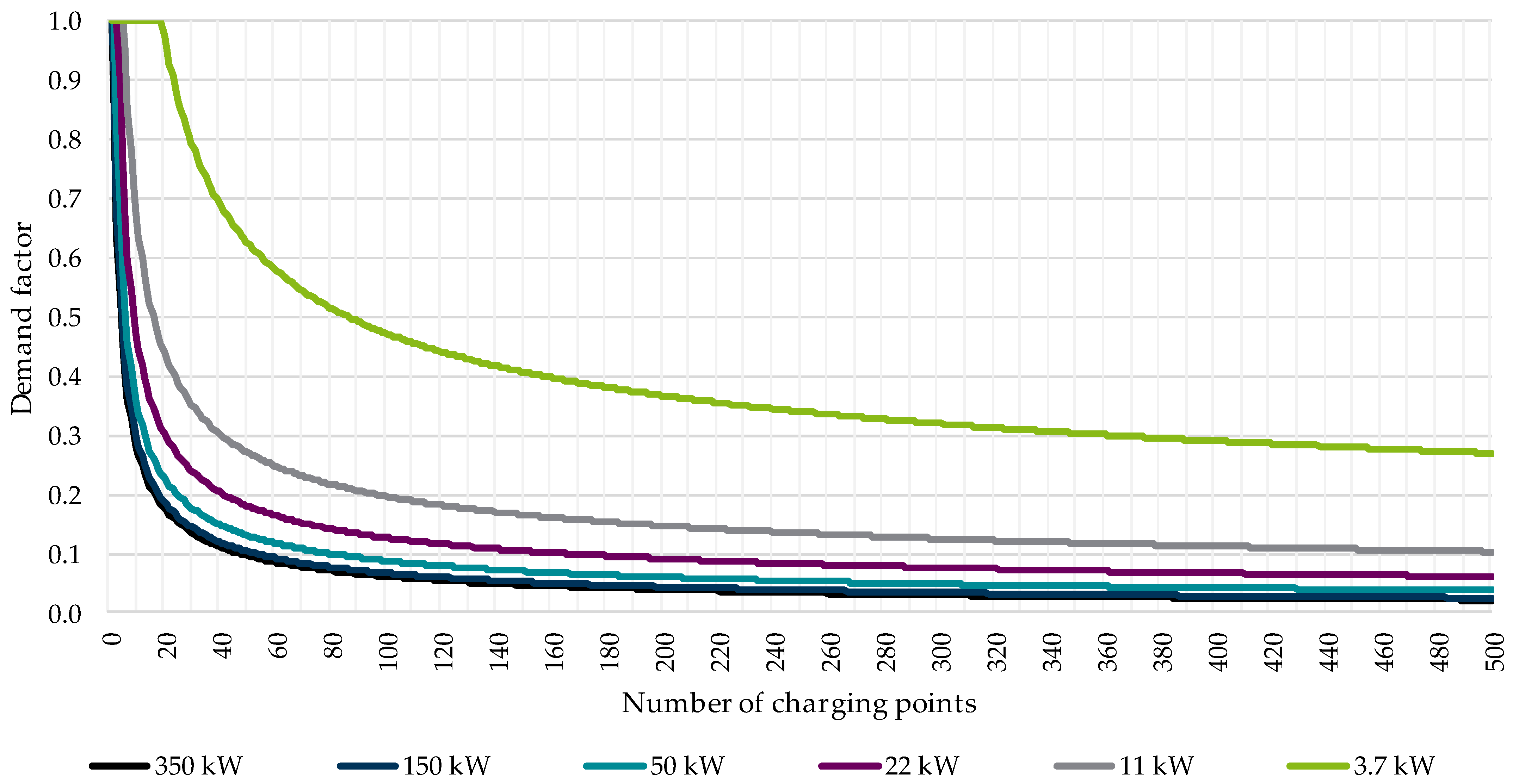
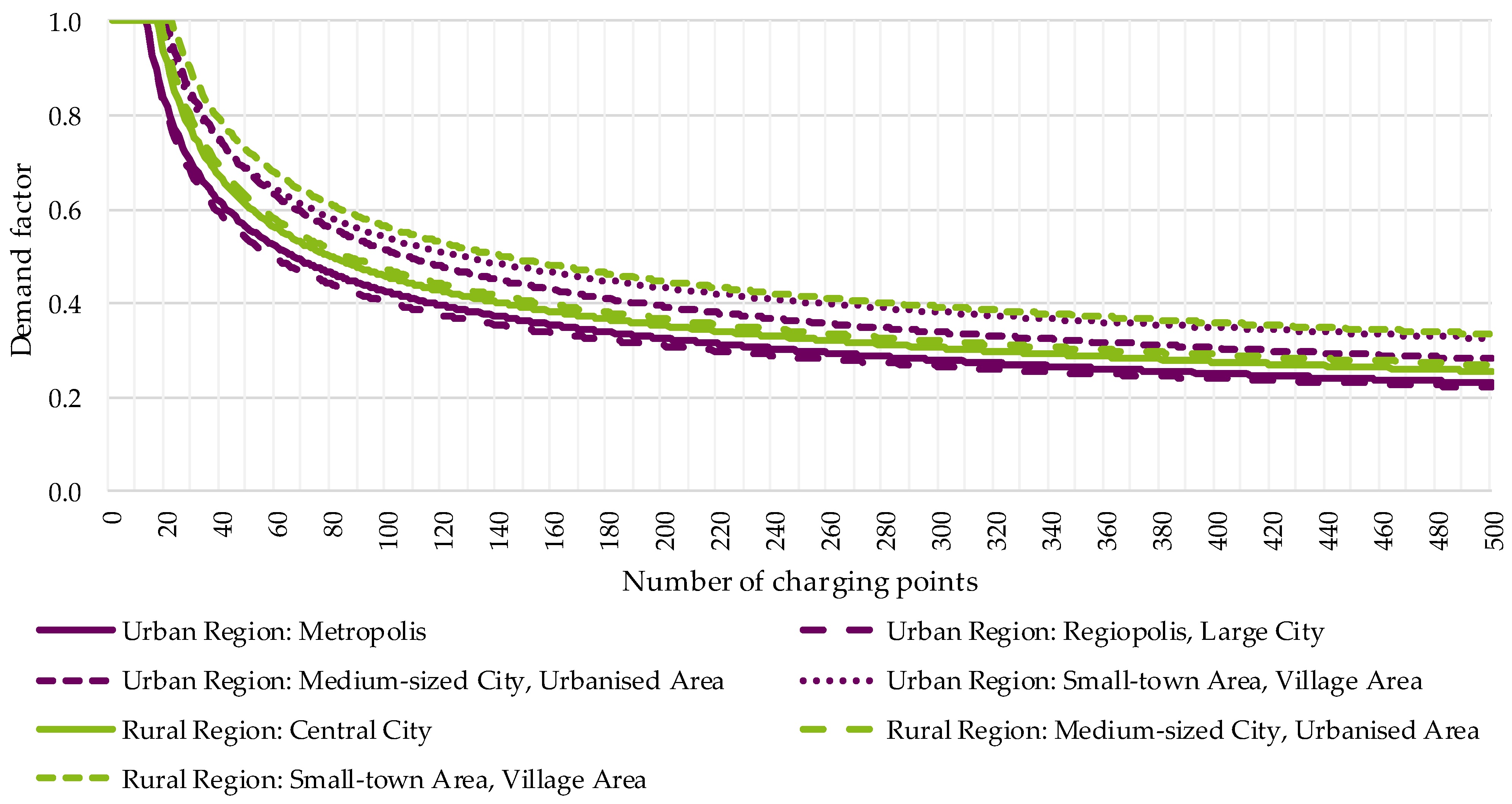
4.2. Demand Factors According to the Charging Powers

For the seven different area types, the DFs can be taken from Figure 18 for 350 kW, Figure 19 for 150 kW, Figure 20 for 50 kW, Figure 21 for 22 kW, Figure 22 for 11 kW, and Figure 23 for 3.7 kW charging power.

Here, it can be seen that the differences in the DFs between the seven area types depend greatly on the charging power, which is particularly noticeable in the explicit data values listed in Appendix B in the Table A1, Table A2, Table A3, Table A4, Table A5, Table A6 and Table A7. It is mentioned in Section 4.1 that the DF values for the charging powers 150 kW up to 350 kW are nearly equal, independent of the charging power. Here, it becomes clear that their DF values also remain nearly equal, independent of the area type. As a consequence, the DF values for the charging powers starting from 150 kW can be generally applied without regarding the explicit charging power or the area type.

By observing Figure 23, a distinction between the area types becomes clear. It can be seen that the “Urban Region: Regiopolis, Large City” has the lowest DF values, even lower than the values for the three other urban region area types. Furthermore, the “Rural Region: Central City” and the “Rural Region: Medium-sized City, Urbanised Area” have lower DF values than the “Urban Region: Medium-sized City, Urbanised Area” and the “Urban Region: Small-town Area, Village Area”. This proves that the DF values for cities are lower than the values for village areas independent of the categorisation, whether it is urban or rural. The same trends are seen for the charging powers of 22 kW and 11 kW in Figure 21 and Figure 22, respectively.

The difference in the DF values between the seven area types becomes clear for the smaller charging powers such as 3.7 kW and 11 kW. Although the difference between the DF values seems negligible, the resulting accumulated charging power varies significantly depending on the area type. Therefore, the resulting accumulated charging powers are presented separately per nominal charging power in Appendix C in the Figure A7, Figure A8, Figure A9, Figure A10, Figure A11 and Figure A12.

5. Discussion

The following two sections discuss the results from Section 4 by first evaluating the influence of the general framework and the method used to determine the DFs. This is followed by a sensitivity analysis with results from other studies.

5.1. Influence of the General Conditions and Evaluation of the Method

The results in Section 4 are based on the database from Section 2 and the assumptions made in Section 3. They essentially depend on the average battery consumption, the chaotic charging and the algorithm for generating probabilistic charging profiles based on the input data for conventional mobility behaviour.

The underlying assumption is that the driving behaviour will not change by changing the driving power from a combustion engine to an electric engine. This assumption is considered to remain valid because the driving behaviour is driven by the individual need for mobility. Since the individual need for mobility is independent of the power source, whether it is fossil fuel or electric, the driving behaviour remains the same in both cases.

Another factor influencing the DF values is battery consumption. If the battery consumption increases, for example, the charging times would increase, thus leading to higher simultaneity and DF values. However, the advancement in battery technology suggests that the battery consumption is actually decreasing ([34]), which can consequently reduce the simultaneity and the DF values.

Similarly, if the available charging time windows are fixed to a certain period of time during the day, the DF values would significantly increase because the charging processes can no longer be distributed over the day.

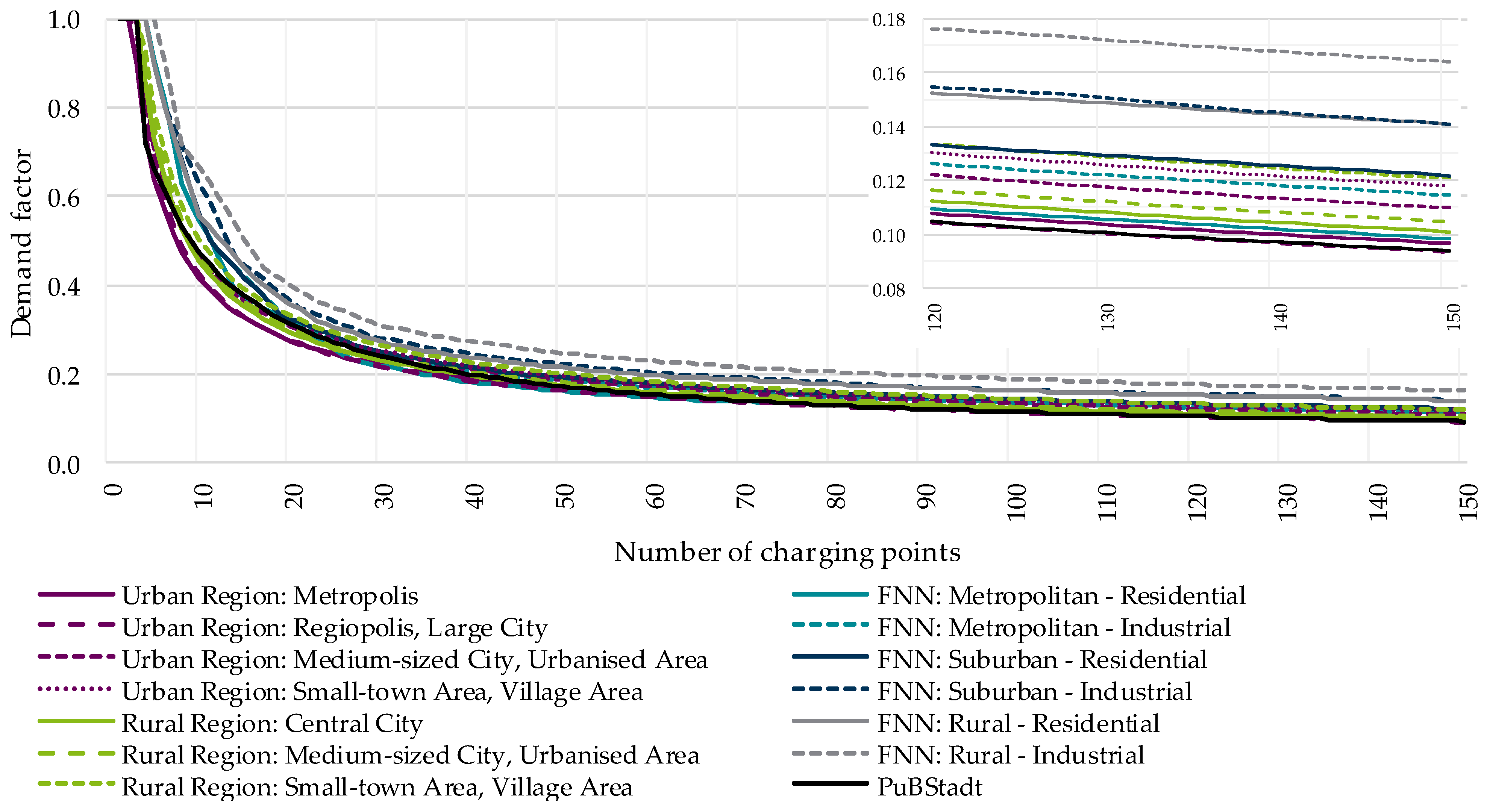
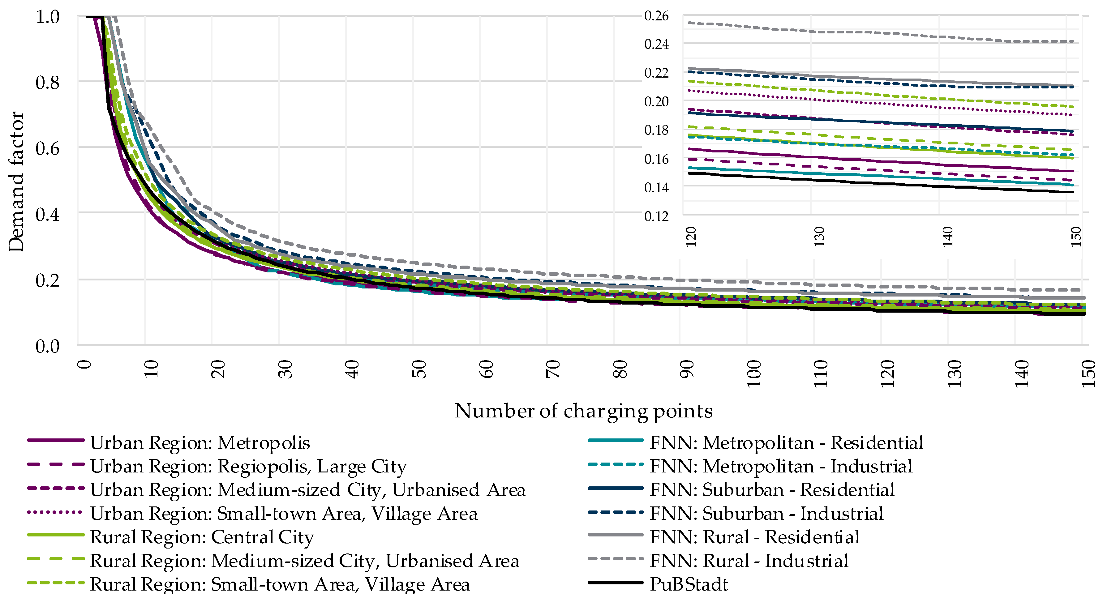
5.2. Sensitivity Analysis to Other Studies

As further validation of the DFs presented in this contribution, a sensitivity analysis with other published studies is carried out. This section compares the results published in this contribution to the results published in the study [35] (abbreviated as “PuBStadt”) and the results published in [17] (referred to as “FNN”). PuBStadt presents DF values to be applied in urban cities without further distinction between the different urban regions. In contrast, FNN introduces three area types which are: metropolitan, suburban and rural. For each of these area types, the area utilisation is split into residential and industrial areas, thus giving a total of six area types. Additionally, FNN provides DF curves for three times of day namely: morning, noon and evening. For the following evaluation, the maximum DF curve for each area type independent of the area utilisation and of the time of day is used.

Similar to the contribution in hand, the FNN employs the database from [27] to generate the DFs. Even though the FNN presumes the distinction between residential and industrial areas, this distinction is originally not available in the database. Hence, a distinction in area utilisation is not considered in this contribution.

Moreover, the consideration of different DF curves for different times of day is applicable when different operating points are considered in strategic grid planning, for instance, a high distributed generation (low load) and/or a high load (low distributed generation) operating point. An operating point is defined as a “point on a characteristic curve representing the values of variable quantities at which a system is operating” [36]. In this case, an operating point refers to the peak points in the electric load profile of a distribution grid. However, since the DF curves serve as an instrument to calculate the maximum expected load (high load operating point) in the grid, the strategic grid planning must dimension the grids to take on this maximum load independent of the time of day. Hence, the generation of DF curves according to the time of day is regarded in this contribution as non-useful.

In addition, the DF curves presented in FNN extend to 150 CPs and not 500 CPs, as the results published in FNN consider only this number of CPs. Figure 11, Figure 12, Figure 13, Figure 14, Figure 15, Figure 16 and Figure 17 clearly demonstrate that the DF values continue decreasing after 150 CPs and start to stagnate around 400 CPs. Hence, it cannot be assumed that the DF curves reach a constant value starting from 150 CPs. Therefore, this limited number of CPs cannot be used for strategic grid planning of medium-voltage grids (or large LV grids), as the number of CPs to be considered is most likely to exceed 150 CPs.

Since the FNN study does not present charging powers higher than 22 kW, the following analyses in Figure 24, Figure 25, Figure 26 and Figure 27 are limited to the charging powers of 11 kW and 22 kW and 150 CPs. Nevertheless, DF curves for 50 kW charging power and higher are needed for the consideration of puCPs in strategic grid planning.

The following Figure 24 and Figure 25 present the DF curves for the charging powers of 11 kW and 22 kW, respectively, for the aforementioned seven area types in comparison to the DF curves from FNN and PuBStadt. At first glance, the DF curves seem to be approximately equal; however, differences between the curves appear in the zoomed-in section in the top right corner of the respective figure.

First of all, the DF curve from PuBStadt overlaps the DF curve for the “Urban Region: Regiopolis, Large City”. Even though PuBStadt displays a single DF curve per charging power, the curves are consistent with the goal of the study since PuBStadt focuses on urban strategic grid planning.

Secondly, the DF curves of FNN for the metropolitan regions (residential and industrial) are between the DF curves for the four urban region area types, which in turn affirms the values presented in this contribution. Remarkably, the DF curves of FNN for the rural regions surpass the DF curves for the rural regions presented in this contribution. This can be due to the assumption made by FNN that EV consumption in rural and suburban areas is higher than in urban areas. This assumption is not considered in this contribution depending on the fact that the driven EVs and the roads are the same in all area types and, therefore, the EV consumption stays equal in all area types. Eventually, the higher values exhibited by the DF curves of the FNN: rural and suburban areas lead to higher accumulated charging powers (see Figure 26 and Figure 27) and, in some cases, can lead to an over-dimensioning of the equipment. Moreover, the DF curves of FNN for the suburban—industrial and the rural—residential regions are nearly equal.

Finally, by focusing on the DF curves of the FNN for a small number of CPs (in the range of 0 up to 20 CPs), an edged curve is noticed, which implies a primitive non-smooth curve fitting method. This is not to be noticed in the DF curves published in this contribution nor the curves published in PuBStadt.

Based on the above presented DF curves, the accumulated charging power for 11 kW and 22 kW charging powers are calculated according to Equation (2).

$$P_{\mathrm{n},\mathrm{p}}=D{F}_{\mathrm{n},\mathrm{p}}·n·p$$

(2)

where P_n,p is the cumulative charging power and DF_n,p is the DF for n CPs of the nominal power p.

The following Figure 26 and Figure 27 illustrate the accumulated charging power curves for the seven area types in comparison to the values from PuBStadt and FNN. As expected, the accumulated charging power values from PuBStadt overlap with the curves for the urban regions presented in this contribution. The aforementioned difference in the DF values for the FNN: rural and suburban regions is reflected here in the accumulated charging powers. For the 22 kW charging power, a difference of approximately 150 kW results between the FNN: rural—industrial area and the “Rural Region: Small-Town Area, Village Area” for 150 CPs. This difference can be seen in the zoomed-in section in the top left corner of the Figure. Within strategic grid planning, this difference can, in some cases, lead to an over-dimensioning of the equipment. The effect of this difference on the final planning measures needs to be proved with further measured data.

6. Conclusions

The contribution in hand utilises the available statistical data using the databases from [26,27] to generate DF curves for seven different area types and for charging powers ranging from 3.7 kW up to 350 kW for up to 500 CPs. The applied method differentiates the area types according to [29] for the generation of probabilistic charging profiles according to [30]. The charging profiles are utilised to calculate the DF values according to [20]. The results for calculating the DFs in Section 4 show that it is essential to apply different DFs depending on the location of the respective grid area (see also Figure 4). The methodically calculated DF values are later on analysed in comparison with similar and independent studies, e.g., [17,35].

In general, the generation of DF curves for the nominal charging powers serves as a practical consideration in the context of strategic grid planning and simplifies the planning process. This has been proven by [25], where a significantly more extensive time series-based grid planning leads to the same results as applying DFs.

The main advantage of the DF curves presented in this contribution is that they provide the ability to perform strategic grid planning while considering a wide range of charging powers extending from 3.7 kW to 350 kW as well as considering the specific area type. In addition, the DF curves are shown for up to 500 CPs and can be applied for even a larger number of CPs, following the characteristic that the DFs remain constant after 500 CPs. To summarise, the DFs can be directly applied in strategic grid planning until a reliable and comprehensive database is available for the measurement of charging processes of different charging powers in different area structures or area types.

The presented DF curves in this contribution and the analyses show the importance of implementing different DF values for the different area types, especially for lower charging powers (3.7 kW and 11 kW). However, it can also be noted that the distinction between the area types is no longer significant for, in particular, higher charging powers of 150 kW and above.

The sensitivity analysis in Section 5.2 has shown that the results introduced here are approximately equal to those of other studies. The negligible difference is essentially justified by slightly different assumptions—in regards to battery consumption—and the results presented in this contribution are, therefore, evaluated as valid.

The analyses performed and results generated for DFs for different charging powers in seven area types serve as a basis for further research work dealing with the topic of electromobility. The DFs presented in the contribution are a result of the simulation tool presented in Section 3 and are based on the driving profiles from [26,27]. In the upcoming years and with the increasing integration of CPs, measurement data can be collected to calculate the DFs and to prove the feasibility of the represented DF curves. Until the measurement data become available, the presented DFs can serve as a practical database for strategic grid planning for different area types and different charging powers up to 350 kW and up to more than 500 CPs.

References

1. IRENA. Rise of Renewables in Cities: Energy Solutions for the Urban Future. 2020. Available online: https://www.irena.org/-/media/Files/IRENA/Agency/Publication/2020/Oct/IRENA_Renewables_in_cities_2020.pdf (accessed on 1 August 2021).
2. Knobloch, F.; Hanssen, S.V.; Lam, A.; Pollitt, H.; Salas, P.; Chewpreecha, U.; Huijbregts, M.A.J.; Mercure, J.-F. Net emission reductions from electric cars and heat pumps in 59 world regions over time. Nat. Sustain. 2020, 3, 437–447. [Google Scholar] [CrossRef] [PubMed]
3. Garcia-Valle, R.; Peças Lopes, J.A. (Eds.) Electric Vehicle Integration into Modern Power Networks; Springer: New York, NY, USA, 2013; ISBN 978-1-4614-0133-9. [Google Scholar] [CrossRef]
4. Bundesministerium für Wirtschaft und Klimaschutz (BMWK). Zweite Verordnung zur Änderung der Ladesäulen-Verordnung, Referentenentwurf der Bundesregierung. 2020. Available online: https://www.bmwk.de/Redaktion/DE/Publikationen/Energie/zweite-verordnung-bmwi-zur-aenderung-der-ladesaeulenverordnung.pdf?__blob=publicationFile&v=2 (accessed on 11 June 2022).
5. Bundesministerium der Justiz. Verordnung über Technische Mindestanforderungen an den Sicheren und Interoperablen Aufbau und Betrieb von Öffentlich Zugänglichen Ladepunkten für Elektrisch Betriebene Fahrzeuge. 2021. Available online: https://www.gesetze-im-internet.de/lsv/BJNR045700016.html (accessed on 11 June 2022).
6. Schlömer, G. Planung von Optimierten Niederspannungsnetzen; Gottfried Wilhelm Leibniz Universität Hannover: Hannover, Germany, 2017; Available online: https://www.repo.uni-hannover.de/handle/123456789/9113 (accessed on 29 July 2021).
7. IEC 60050—International Electrotechnical Vocabulary—Details for IEV Number 691-10-05: “Demand Factor”. Available online: https://www.electropedia.org/iev/iev.nsf/display?openform&ievref=691-10-05 (accessed on 20 June 2022).
8. Arif, S.M.; Lie, T.T.; Seet, B.C.; Ayyadi, S.; Jensen, K. Review of Electric Vehicle Technologies, Charging Methods, Standards and Optimization Techniques. Electronics 2021, 10, 1910. [Google Scholar] [CrossRef]
9. Capasso, A.; Grattieri, W.; Lamedica, R.; Prudenzi, A. A bottom-up approach to residential load modeling. IEEE Trans. Power Syst. 1994, 9, 957–964. [Google Scholar] [CrossRef]
10. Paatero, J.V.; Lund, P.D. A model for generating household electricity load profiles. Int. J. Energy Res. 2006, 30, 273–290. [Google Scholar] [CrossRef]
11. Fischer, D.; Härtl, A.; Wille-Haussmann, B. Model for electric load profiles with high time resolution for German households. Energy Build. 2015, 92, 170–179. [Google Scholar] [CrossRef]
12. Tjaden, T.; Bergner, J.; Weniger, J.; Quaschning, V. Representative Electrical Load Profiles of Residential Buildings in Germany with a Temporal Resolution of One Second. 2015. Available online: https://www.researchgate.net/publication/285577915_Representative_electrical_load_profiles_of_residential_buildings_in_Germany_with_a_temporal_resolution_of_one_second#fullTextFileContent (accessed on 20 June 2022).
13. Mosquet, X.; Zablit, H.; Dinger, A.; Xu, G.; Andersen, M.; Tominaga, K. The Electric Car Tipping Point—The Future of Powertrains for Owned and Shared Mobility. 2018. Available online: https://web-assets.bcg.com/ef/8b/007df7ab420dab1164e89d0a6584/bcg-the-electric-car-tipping-point-jan-2018.pdf (accessed on 1 July 2021).
14. Electric Vehicle Outlook 2018, BloombergNEF, 2018. Available online: https://about.bnef.com/electric-vehicle-outlook/#_toc-download (accessed on 29 July 2021).
15. RBC Electric Vehicle Forecast through 2050 & Primer, RBC Capital Markets. 2018. Available online: http://www.fullertreacymoney.com/system/data/files/PDFs/2018/May/14th/RBC%20Capital%20Markets_RBC%20Electric%20Vehicle%20Forecast%20Through%202050%20%20Primer_11May2018.pdf (accessed on 29 July 2021).
16. Netze BW GmbH. Die e-Mobility-Allee—Das Stromnetz-Reallabor zur Erforschung des Zukünftigen e-Mobility-Alltags; Netze BW GmbH: Stuttgart, Germany, November 2019; Available online: https://assets.ctfassets.net/xytfb1vrn7of/6gXs8wiRSF0E2SqkwSq406/fc1c9430ba88b81c31e399242b09b17e/20191217_BroschuereE-Mobility_210x275mm_100Ansicht.pdf (accessed on 11 June 2022).
17. Forum Netztechnik/Netzbetrieb im VDE (FNN). Ermittlung von Gleichzeitigkeitsfaktoren für Ladevorgänge an Privaten Ladepunkten—Wissenschaftliche Untersuchung zur Gleichzeitigkeit von Ungesteuerten Ladevorgängen von Elektrofahr-Zeugen; VDE-Verlag GmbH: Berlin, Germany, 2021. [Google Scholar]
18. Bollerslev, J.; Andersen, P.B.; Jensen, T.V.; Marinelli, M.; Thingvad, A.; Calearo, L.; Weckesser, T. Coincidence Factors for Domestic EV Charging from Driving and Plug-In Behavior. IEEE Trans. Transp. Electrif. 2022, 8, 808–819. [Google Scholar] [CrossRef]
19. Kreutmayr, S.; Storch, D.J.; Niederle, S.; Steinhart, C.J.; Gutzmann, C.; Finkel, M.; Witzmann, R. Time-Dependent and Location-Based Analysis of Power Consumption at Public Charging Stations in Urban Areas. In Proceedings of the CIRED 2021—The 26th International Conference and Exhibition on Electricity Distribution, Institution of Engineering and Technology, Online Conference, 20–23 September 2021; pp. 2386–2390. [Google Scholar] [CrossRef]
20. Ali, S.; Wintzek, P.; Zdrallek, M.; Böse, C.; Monscheidt, J.; Gemsjäger, B.; Slupinski, A. Demand factor identification of electric vehicle charging points for distribution system planning. In Proceedings of the CIRED 2021—The 26th International Conference and Exhibition on Electricity Distribution, Institution of Engineering and Technology, Online Conference, 20–23 September 2021; pp. 2574–2578. [Google Scholar] [CrossRef]
21. DIN EN 60076-1:2012-03 VDE 0532-76-1:2012-03; Power Transformers—Part 1: General (IEC 60076-1:2011); German Version EN 60076-1:2011. Beuth Verlag GmbH: Berlin, Germany, 2012.
22. DIN EN 50588-1:2019-12; Medium Power Transformers 50 Hz, with Highest Voltage for Equipment Not Exceeding 36 kV—Part 1: General Requirements; German Version EN 50588-1:2017. Beuth Verlag GmbH: Berlin, Germany, 2019.
23. DIN VDE 0276-1000:1995-06; Power Cables; Current-Carrying Capacity, General; Conversion Factors. Beuth Verlag GmbH: Berlin, Germany, 1995.
24. DIN EN 50160:2020-11; Voltage Characteristics of Electricity Supplied by Public Electricity Networks; German Version EN 50160:2010 + Cor.:2010 + A1:2015 + A2:2019 + A3:2019. Beuth Verlag GmbH: Berlin, Germany, 2020.
25. Wintzek, P.; Ali, S.A.; Riedlinger, T.; Düsterhus, P.; Zdrallek, M. Sensitivity Analysis for Different Calculation Methods of Simultaneity Factors for Charging Infrastructure in Low-Voltage Grids. In Proceedings of the CIRED 2022 Workshop, Porto, Portugal, 2–3 June 2021; p. 0470. [Google Scholar]
26. Follmer, R.; Gruschwitz, D.; Jesske, B.; Quandt, S.; Lenz, B.; Nobis, C.; Köhler, K.; Mehlin, M. Mobilität in Deutschland 2008; Ergebnisbericht: Struktur-Aufkommen-Emissionen-Trends; Federal Ministry for Digital and Transport: Bonn, Germany; Berlin, Germany, 2010; Available online: http://www.mobilitaet-in-deutschland.de/pdf/infas_MiD2008_Abschlussbericht_I.pdf (accessed on 24 February 2022).
27. Follmer, R. Mobility in Germany: Short Report Transport Volume-Structure-Trends. 2019. Available online: https://www.bmvi.de/SharedDocs/DE/Anlage/G/mid-2017-short-report.pdf?__blob=publicationFile (accessed on 11 June 2022).
28. Zdrallek, M. Elektromobilität in der Netzplanung—Strategien für Ladeinfrastruktur, Anwendungsfälle und Praxisbeispiele. 2020. Available online: https://www.evt.uni-wuppertal.de/fileadmin/Abteilung/EEV/pdf/aktuelles/Einladungskarte_Web-Seminar_ENP.PDF (accessed on 11 June 2022).
29. RegioStaR: Regional Statistical Spatial Typology for Mobility and Transport Research. 2018. Available online: https://www.bmvi.de/SharedDocs/DE/Anlage/G/regiostar-raumtypologie-englisch.pdf?__blob=publicationFile (accessed on 11 June 2022).
30. Uhlig, R.; Stotzel, M.; Zdrallek, M.; Neusel-Lange, N. Dynamic grid support with EV charging management considering user requirements. In Proceedings of the CIRED Workshop 2016, Institution of Engineering and Technology, Helsinki, Finland, 14–15 June 2016; p. 0071. [Google Scholar] [CrossRef] [Green Version]
31. Müller, T.; Ali, S.A.; Becker, M.; Möller, C.; Zdrallek, M.; Boden, E.; Knoll, C. Impact of different electric vehicle charging models on distribution grid planning. In Proceedings of the CIRED 2021—The 26th International Conference and Exhibition on Electricity Distribution, Institution of Engineering and Technology, Online Conference, 20–23 September 2021; pp. 2396–2400. [Google Scholar] [CrossRef]
32. The MathWorks, Inc. List of Library Models for Curve and Surface Fitting. Available online: https://de.mathworks.com/help/curvefit/list-of-library-models-for-curve-and-surface-fitting.html (accessed on 1 June 2022).
33. Liu, L. Einfluss der Privaten Elektrofahrzeuge auf Mittel- und Niederspannungsnetze. 2018. Available online: https://tuprints.ulb.tu-darmstadt.de/7171/1/Liu_Diss_2018e.pdf (accessed on 20 June 2022).
34. Scrosati, B.; Garche, J.; Tillmetz, W. (Eds.) Advances in Battery Technologies for Electric Vehicles; Woodhead Publishing: Cambridge, UK, 2015; ISBN 978-1-78242-398-0. [Google Scholar]
35. Wintzek, P.; Ali, S.A.; Zdrallek, M.; Monscheidt, J.; Gemsjäger, B.; Slupinski, A. Development of planning and operation guidelines for strategic grid planning of urban low-voltage grids with a new supply task. Electricity 2021, 2, 614–652. [Google Scholar] [CrossRef]
36. IEC 60050—International Electrotechnical Vocabulary—Details for IEV Number 351-45-12: “Operating Point”; International Electrotechnical Commission: London, UK, 2006.
Figure 1. Planning perspectives considering the respective demand factor (DF) [25].
Electricity 03 00022 g001
Figure 2. Left: Probability distribution of the number of routes per day and vehicle. Right: Percentage of the purpose of the daily routes for different weekdays based on [28].
Electricity 03 00022 g002
Figure 3. Left: Probability distribution of the length of the routes per vehicle according to the purpose of the route. Right: Probability distribution of the time of departure of a vehicle according to the purpose of the route based on data published in [27] for “Urban Region: Metropolis”.
Electricity 03 00022 g003
Figure 4. Geographical representation of the seven area types (RegioStar 7) in Germany for the research in mobility and transportation sectors [29], with permission from Federal Ministry of Transport and Digital Infrastructure, 2018.
Electricity 03 00022 g004
Figure 5. Simulation algorithm for generating probabilistic driving and load profiles [28].
Electricity 03 00022 g005
Figure 6. Exemplary weekly charging profile for an electric vehicle and the accumulated charging profile for ten electric vehicles [28].
Electricity 03 00022 g006
Figure 7. Example of calculated demand factors for six charging powers.
Electricity 03 00022 g007
Figure 8. Process diagram for the simulation of charging profiles for different area types and charging powers.
Electricity 03 00022 g008
Figure 9. Example of curve fitting (CF) for charging powers between 3.7 kW and 350 kW for (10, 50, 100 and 500) charging points (CP).
Electricity 03 00022 g009
Figure 10. Example for the newly generated demand factors.
Electricity 03 00022 g010
Figure 11. Demand factors (ordinate) for the area type “Urban Region: Metropolis” and six charging powers.
Electricity 03 00022 g011
Figure 12. Demand factors (ordinate) for the area type “Urban Region: Regiopolis, Large City” and six charging powers.
Electricity 03 00022 g012
Figure 13. Demand factors (ordinate) for the area type “Urban Region: Medium-sized City, Urbanised Area” and six charging powers.
Electricity 03 00022 g013
Figure 14. Demand factors (ordinate) for the area type “Urban Region: Small-town Area, Village Area” and six charging powers.
Electricity 03 00022 g014
Figure 15. Demand factors (ordinate) for the area type “Rural Region: Central City” and six charging powers.
Electricity 03 00022 g015
Figure 16. Demand factors (ordinate) for the area type “Rural Region: Medium-sized City, Urbanised Area” and six charging powers.
Electricity 03 00022 g016
Figure 17. Demand factors (ordinate) for the area type “Rural Region: Small-town Area, Village Area” and six charging powers.
Electricity 03 00022 g017
Figure 18. Demand factors (ordinate) for 350 kW charging power and seven different area types.
Electricity 03 00022 g018
Figure 19. Demand factors (ordinate) for 150 kW charging power and seven different area types.
Electricity 03 00022 g019
Figure 20. Demand factors (ordinate) for 50 kW charging power and seven different area types.
Electricity 03 00022 g020
Figure 21. Demand factors (ordinate) for 22 kW charging power and seven different area types.
Electricity 03 00022 g021
Figure 22. Demand factors (ordinate) for 11 kW charging power and seven different area types.
Electricity 03 00022 g022
Figure 23. Demand factors (ordinate) for 3.7 kW charging power and seven different area types.
Electricity 03 00022 g023
Figure 24. Demand factors (ordinate) for 22 kW charging power with seven different area types, six area types according to FNN and the results from PuBStadt for 150 charging points.
Electricity 03 00022 g024
Figure 25. Demand factors (ordinate) for 11 kW charging power with seven different area types, six area types according to FNN and the results from PuBStadt for 150 charging points.
Electricity 03 00022 g025
Figure 26. Accumulated charging power (ordinate) for 22 kW charging power with seven different area types, six area types according to FNN and the results from PuBStadt for 150 charging points.
Electricity 03 00022 g026
Figure 27. Accumulated charging power (ordinate) for 11 kW charging power with seven different area types, six area types according to FNN and the results from PuBStadt for 150 charging points.
Electricity 03 00022 g027
Publisher’s Note: MDPI stays neutral with regard to jurisdictional claims in published maps and institutional affiliations.