Parameter Identification Concept for Process Models Combining Systems Theory and Deep Learning ^†

Abstract

In recent years, dynamic process models have grown even more important in the context of Industry 4.0 and the use of digital twins. However, the accuracy of the corresponding model parameter estimates is determined by the quantity and quality of data and the parameter identification solving methodologies used. Standard methods are based on the ordinary least squares framework. Still, other options are available that might be more sensitive to model parameter variations and ensure more precise parameter estimates. The paper presents a novel technique for parameter identification based on incorporating neural ordinary differential equations for surrogate modeling and differential flatness, i.e., a systems theory concept in control engineering. This approach may lead to improved parameter sensitivities, as demonstrated with a simulation study of a distributed-parameter identification problem assuming a diffusion-type parabolic partial differential equation.

1. Introduction

System identification is the process of creating a mathematical model, or equation, to represent a real-world problem. This equation can then be used to predict and analyze possible outcomes of the system under study. In many engineering fields, the time behavior of complicated technical systems can be described by using a system of ordinary differential equations (ODEs). However, the parameters in these equations are often unknown and need to be estimated from experimental data. Over the past few decades, there has been intense research on parameter estimation methods. A popular method minimizes the sum of squared errors (SSE) between a model prediction and measurement data, where the prediction is calculated by solving the ODE numerically [1]. The model parameters are then adjusted until a given minimization criterion is reached. However, other options are available that might be more sensitive to model parameter variations and might ensure more precise parameter estimates, respectively. Control and systems theory can improve parameter identification procedures, e.g., online parameter identification concepts [2,3].

Another example is differential flatness to recalculate control trajectory profiles for desired system dynamics [4,5], i.e., following a system inversion concept. In a differential flat system, state variables and input variables can be expressed as functions of so-called flat outputs and a finite number of their derivatives, also leading to a reformulation of the parameter identification problem. Moreover, while optimal experimental design concepts might be needed to improve data quantity and quality [3], the flatness concepts involved in the flat output approach may result in improved parameter sensitivities [6] and more precise parameter estimates [7,8] without experimental data enrichment.

2. Methods

2.1. Parameter Identification Problem

Frequently, dynamic process models are given as ordinary differential equation systems:

$$\begin{array}{c}\dot{\mathrm{x}}\left(\mathrm{t}\right)=\mathrm{f}\left(\mathrm{x}\left(\mathrm{t}\right),\mathrm{u}\left(\mathrm{t}\right),\mathrm{p}\right),\\ \mathrm{x}\left({\mathrm{t}}_0\right)={\mathrm{x}}_0,\end{array}$$

(1)

where $\mathrm{t}\in \left[{\mathrm{t}}_0,{\mathrm{t}}_0+{\mathrm{t}}_{\mathrm{end}}\right]$ is the time, with ${\mathrm{t}}_0$ as the initial time and ${\mathrm{t}}_{\mathrm{end}}$ as the time duration of the simulation, $\mathrm{u}\in {\mathrm{R}}^{{\mathrm{n}}_{\mathrm{u}}}$ is the vector of the control variables, $\mathrm{p}\in {\mathrm{R}}^{{\mathrm{n}}_{\mathrm{p}}}$ is the vector of the time-invariant parameters, and ${\mathrm{x}}_{}\in {\mathrm{R}}^{{\mathrm{n}}_{\mathrm{x}}}$ are the differential system states. The initial conditions for the differential states are given by ${\mathrm{x}}_0$. Moreover, $\mathrm{f}:{\mathrm{R}}^{{\mathrm{n}}_{\mathrm{x}}\times {\mathrm{n}}_{\mathrm{u}}\times {\mathrm{n}}_{\mathrm{p}}}\to {\mathrm{R}}^{{\mathrm{n}}_{\mathrm{x}}}$ represents the corresponding vector field. For this kind of mathematical representation, the standard approach of parameter identification, i.e., the ordinary least squares (OLS) method, can be defined as:

$${\widehat{\mathrm{p}}}^{\mathrm{OLS}}=arg\underset{\mathrm{p}}{min}{\sum }_{\mathrm{k}=1}^{\mathrm{K}}{∥{\mathrm{y}}^{\mathrm{data}}\left(t_k\right)-\mathrm{y}\left(t_k,\mathrm{p}\right)∥}_2^2,$$

(2)

where $||\cdot |{|}_2$ denotes the Euclidean norm, ${\mathrm{y}}^{\mathrm{data}}\left(t_k\right)$ represents the data vector at discrete time points $t_k$ over all measurement samples $\mathrm{K},$ and the model output function is defined as:

$$\mathrm{y}\left(t_k,\mathrm{p}\right)=\mathrm{h}\left(\mathrm{x}\left(t_k,\mathrm{p}\right)\right),$$

(3)

with $\mathrm{h}:{\mathrm{R}}^{{\mathrm{n}}_{\mathrm{x}}}\to {\mathrm{R}}^{{\mathrm{n}}_{\mathrm{y}}}$, and $\mathrm{y}\in {\mathrm{R}}^{{\mathrm{n}}_{\mathrm{y}}}$ as the model output vector. Alternatively, when aiming to utilize the inverse model response, i.e., applying a model inversion strategy, an input least squares (ILS)-based parameter identification problem can be used:

$${\widehat{\mathrm{p}}}^{\mathrm{ILS}}={\sum }_{\mathrm{k}=1}^{\mathrm{K}}{∥{\mathrm{u}}^{\mathrm{data}}\left(t_k\right)-\mathrm{u}\left(t_k,\mathrm{p}\right)∥}_2^2.$$

(4)

Here, the control inputs, $\mathrm{u}\left(t_k,\mathrm{p}\right)$, have to be calculated to solve the parameter identification problem, and ${\mathrm{u}}^{\mathrm{data}}\left(t_k\right)$ represents the recorded physical input actions. For this purpose, we study the differential flatness concept outlined in Section 2.2. However, it is essential to note that parameter sensitivities are relevant for well-posed parameter identification problems. On having the output function $\mathrm{y}\left(t_k,\mathrm{p}\right)$ and the inputs $\mathrm{u}\left(t_k,\mathrm{p}\right)$ (inverse model response), the sensitivity $\mathrm{S}$ of the parameter $\mathrm{p}$ is defined as:

$${\mathrm{S}}_{{\mathrm{y}}_{\mathrm{p}}}\left(t_k\right)=\frac{\partial \mathrm{y}\left(t_k,\mathrm{p}\right)}{\partial \mathrm{p}},$$

(5)

$${\mathrm{S}}_{{\mathrm{u}}_{\mathrm{p}}}\left(t_k\right)=\frac{\partial \mathrm{u}\left(t_k,\mathrm{p}\right)}{\partial \mathrm{p}}.$$

(6)

Here, in general, absolute high parameter sensitivity values ensure precise parameter estimates according to the Fisher Information matrix and the Cramér Rao inequality [1,3].

2.2. Differential Flatness

In literature, a process model (Equation (1)) is called differentially flat if there is an output function:

$${\mathrm{y}}^{\mathrm{flat}}={\mathrm{h}}^{\mathrm{flat}}\left(\mathrm{x},\mathrm{u},\dot{\mathrm{u}},\dots ,{\mathrm{u}}^{\left(\mathrm{s}\right)},\mathrm{p}\right),$$

(7)

with a finite value $\mathrm{s}\in \mathrm{N}$ and the smooth mapping function ${\mathrm{y}}^{\mathrm{flat}}:{\mathrm{R}}^{{\mathrm{n}}_{\mathrm{x}}}\times {\left({\mathrm{R}}^{{\mathrm{n}}_{\mathrm{u}}}\right)}^{\mathrm{s}+1}\times {\mathrm{R}}^{{\mathrm{n}}_{\mathrm{p}}}\to {\mathrm{R}}^{{\mathrm{n}}_{\mathrm{y}}}$ that is called flat output. With the flat output, the system states and control inputs are expressed as:

$$\mathrm{x}={\mathsf{\Psi }}_{\mathrm{x}}\left({\mathrm{y}}^{\mathrm{flat}},{\dot{\mathrm{y}}}^{\mathrm{flat}},\dots ,{\mathrm{y}}^{{\mathrm{flat}}^{\left(\mathrm{r}\right)}},\mathrm{p}\right),$$

(8)

$$\mathrm{u}={\mathsf{\Psi }}_{\mathrm{u}}\left({\mathrm{y}}^{\mathrm{flat}},{\dot{\mathrm{y}}}^{\mathrm{flat}},\dots ,{\mathrm{y}}^{{\mathrm{flat}}^{\left(\mathrm{r}+1\right)}},\mathrm{p}\right),$$

(9)

with the mapping functions ${\mathsf{\Psi }}_{\mathrm{x}}:{\left({\mathrm{R}}^{{\mathrm{n}}_{\mathrm{y}}}\right)}^{\mathrm{r}+1}\times {\mathrm{R}}^{{\mathrm{n}}_{\mathrm{p}}}\to {\mathrm{R}}^{{\mathrm{n}}_{\mathrm{x}}}$ and ${\mathsf{\Psi }}_{\mathrm{u}}:{\left({\mathrm{R}}^{{\mathrm{n}}_{\mathrm{y}}}\right)}^{\mathrm{r}+2}\times {\mathrm{R}}^{{\mathrm{n}}_{\mathrm{p}}}\to {\mathrm{R}}^{{\mathrm{n}}_{\mathrm{u}}}$, and assuming a quadratic system ${\mathrm{dimy}}^{\mathrm{flat}}=\mathrm{dimu}.$ When applying the flatness concept, it was shown that parameter sensitivities and the reliability of parameter estimates, respectively, could be improved in the case of ILS [6] or when combining the OLS with ILS [7,8]. However, in process systems engineering, for instance, besides lumped-parameter systems (i.e., ordinary differential equations), distributed-parameter systems, described via partial differential equations, are frequently applied. In this case, the differential flatness approach has to be generalized [5,9,10,11].

2.3. Neural Ordinary Differential Equations

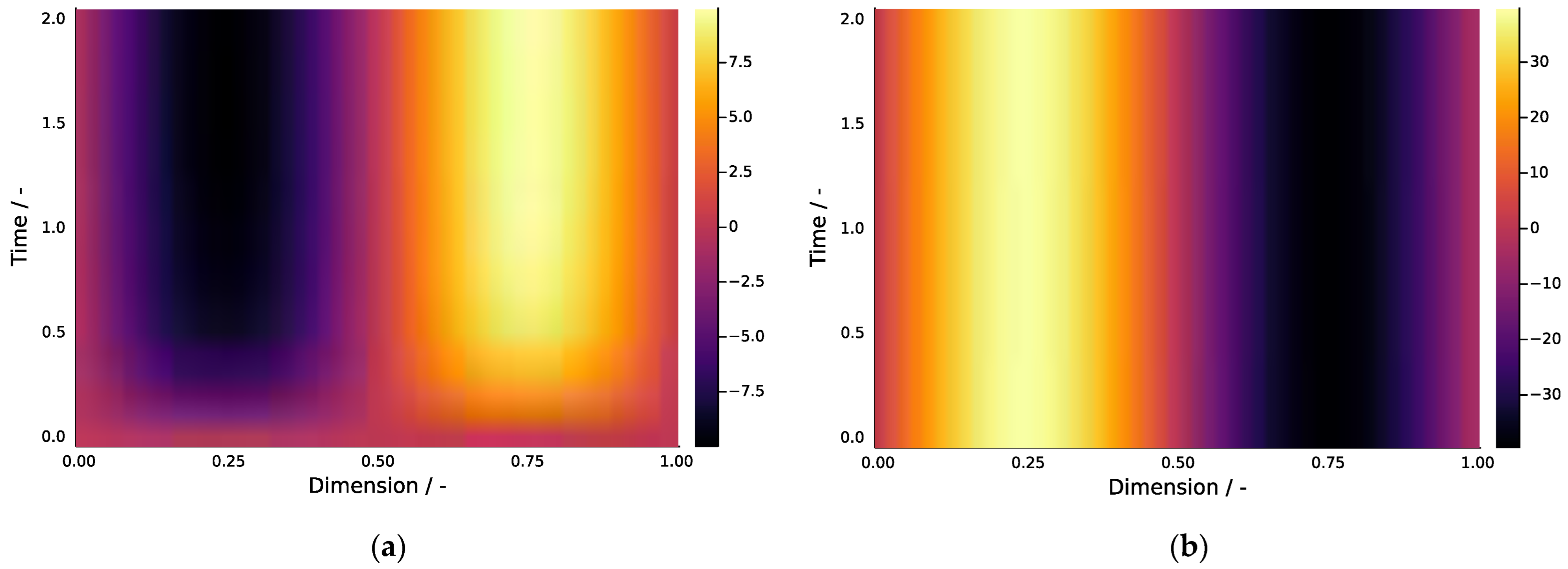
In data science and deep learning, neural networks are frequently used to build empirical models. A neural network is a group of interconnected neurons with one or more hidden layers depending on the network’s specific task. Technically, the $i^{th}$ neural network layer, $NN{L}_i\left(x\right): R^{d_{i-1}}\to R^{d_i}$, contains $N_i$ neurons. Here, $NN{L}_i\left(x\right)$ is specified with the weight matrix, $W^i\in R^{d_i\times d_{i-1}}$, and the bias vector, $b_i\in R^{d_i}.$ Thus, for instance, a feed-forward neural network reads as:

$$\begin{array}{c}{\mathrm{NNL}}_0\left(\mathrm{x}\right)=\mathrm{x}\in {\mathrm{R}}^{{\mathrm{d}}_0},\\ {\mathrm{NNL}}_{\mathrm{j}}\left(\mathrm{x}\right)=\mathsf{\sigma }\left({\mathrm{W}}^{\mathrm{j}}{\mathrm{NNL}}_{\mathrm{j}-1}\left(\mathrm{x}\right)+{\mathrm{b}}_{\mathrm{j}}\right)\in {\mathrm{R}}^{{\mathrm{d}}_{\mathrm{j}}}\\ \hspace{1em}\hspace{1em}\hspace{1em}\hspace{1em}\hspace{1em}\forall 1\le \mathrm{j}\le \mathrm{I}-1\\ {\mathrm{NNL}}_{\mathrm{I}}\left(\mathrm{x}\right)={\mathrm{W}}^{\mathrm{I}}{\mathrm{NNL}}_{\mathrm{I}-1}\left(\mathrm{x}\right)+{\mathrm{b}}_{\mathrm{I}}\in {\mathrm{R}}^{{\mathrm{d}}_{\mathrm{I}}}.\end{array},$$

(10)

When it comes to the so-called neural ordinary differential equations, the governing equations read as:

$$\dot{\mathrm{x}}\left(\mathrm{t}\right)=\mathrm{NN}\left(\mathrm{x}\left(\mathrm{t}\right),\mathrm{u}\left(\mathrm{t}\right),\mathrm{p}\right),\mathrm{x}\left({\mathrm{t}}_0\right)={\mathrm{x}}_0.$$

(11)

Neural ODEs offer a promising approach for hybrid modeling and system identification [12,13,14,15]. Furthermore, the neural network’s architecture can be optimized to represent experimental data better. This could be performed in conjunction with optimal experimental design methods [3] to improve the accuracy of system identification further.

3. Case Study

Determining kinetic parameters of (diffusion-type parabolic) PDEs (e.g., Equation (12)) has been extensively studied, including chromatography and adsorption processes [2,16,17,18,19], respectively.

$$\frac{\partial \mathsf{\varphi }}{\partial \mathrm{t}}=\mathrm{p}\frac{{\partial }^2\mathsf{\varphi }}{\partial {\mathrm{x}}^2}+\mathrm{u}\left(\mathrm{x},\mathrm{t}\right)$$

(12)

Following the numerical solution and the finite difference method (Equation (13)) of the diffusion-type PDE, a set of coupled ODEs is obtained, which can be written in the state-space form as shown in Equation (14).

$$\frac{{\partial }^2\mathsf{\varphi }}{\partial {\mathrm{x}}^2}\simeq \frac{{\mathsf{\varphi }}_{\mathrm{i}+1}-2{\mathsf{\varphi }}_{\mathrm{i}}+{\mathsf{\varphi }}_{\mathrm{i}-1}}{{\Delta \mathrm{x}}^2}$$

(13)

$$\begin{array}{c}\frac{\partial {\mathsf{\varphi }}_1}{\partial \mathrm{t}}=\frac{\mathrm{p}}{\Delta {\mathrm{x}}^2}{\mathsf{\varphi }}_2-\frac{2\mathrm{p}}{\Delta {\mathrm{x}}^2}{\mathsf{\varphi }}_1+\frac{\mathrm{p}}{\Delta {\mathrm{x}}^2}{\mathsf{\varphi }}_0+{\mathrm{u}}_1\left(\mathrm{t}\right),\\ \frac{\partial {\mathsf{\varphi }}_2}{\partial \mathrm{t}}=\frac{\mathrm{p}}{\Delta {\mathrm{x}}^2}{\mathsf{\varphi }}_3-\frac{2\mathrm{p}}{\Delta {\mathrm{x}}^2}{\mathsf{\varphi }}_2+\frac{\mathrm{p}}{\Delta {\mathrm{x}}^2}{\mathsf{\varphi }}_1+{\mathrm{u}}_2\left(\mathrm{t}\right),\\ \frac{\partial {\mathsf{\varphi }}_3}{\partial \mathrm{t}}=\frac{\mathrm{p}}{\Delta {\mathrm{x}}^2}{\mathsf{\varphi }}_4-\frac{2\mathrm{p}}{\Delta {\mathrm{x}}^2}{\mathsf{\varphi }}_3+\frac{\mathrm{p}}{\Delta {\mathrm{x}}^2}{\mathsf{\varphi }}_2+{\mathrm{u}}_3\left(\mathrm{t}\right),\\ \cdots \\ \frac{\partial {\mathsf{\varphi }}_{\mathrm{N}-1}}{\partial \mathrm{t}}=\frac{\mathrm{p}}{\Delta {\mathrm{x}}^2}{\mathsf{\varphi }}_{\mathrm{N}}-\frac{2\mathrm{p}}{\Delta {\mathrm{x}}^2}{\mathsf{\varphi }}_{\mathrm{N}-1}+\frac{\mathrm{p}}{\Delta {\mathrm{x}}^2}{\mathsf{\varphi }}_{\mathrm{N}-2}+{\mathrm{u}}_{\mathrm{N}-1}\left(\mathrm{t}\right),\\ \frac{\partial {\mathsf{\varphi }}_{\mathrm{N}}}{\partial \mathrm{t}}=\frac{\mathrm{p}}{\Delta {\mathrm{x}}^2}{\mathsf{\varphi }}_{\mathrm{N}+1}-\frac{2\mathrm{p}}{\Delta {\mathrm{x}}^2}{\mathsf{\varphi }}_{\mathrm{N}}+\frac{\mathrm{p}}{\Delta {\mathrm{x}}^2}{\mathsf{\varphi }}_{\mathrm{N}-1}+{\mathrm{u}}_{\mathrm{N}}\left(\mathrm{t}\right),\end{array}.$$

(14)

Practically, the parameter identification problem for this academic case study is to determine the diffusion parameter $\mathrm{p}$ in this system to represent the actual physical process being modeled accurately. This can be challenging as even minor changes in the coefficient value can result in significant changes in solution behavior or vice versa. However, it is often possible to obtain reasonable estimates for the diffusion parameter with careful analysis and experimentation [2,18], including the proposed concept of combining systems theory with differential flatness and deep learning. In particular, when assuming that all states in Equation (14) are measurable, i.e., ${\mathrm{y}}_{\mathrm{i}}={\mathsf{\varphi }}_{\mathrm{i}},\forall 1\le \mathrm{i}\le \mathrm{N},$ and that the output derivatives, i.e., ${\dot{\mathrm{y}}}_{\mathrm{i}},\forall 1\le \mathrm{i}\le \mathrm{N},$ exist, then the related equation system (Equation (15)) can be transformed to determine the input variables, ${\mathrm{u}}_{\mathrm{i}},\forall 1\le \mathrm{i}\le \mathrm{N}$, accordingly.

$$\begin{array}{c}\left(\begin{array}{c}{\dot{\mathrm{y}}}_1\left(\mathrm{t}\right)\\ {\dot{\mathrm{y}}}_2\left(\mathrm{t}\right)\\ \cdots \\ {\dot{\mathrm{y}}}_{\mathrm{N}-1}\left(\mathrm{t}\right)\\ {\dot{\mathrm{y}}}_{\mathrm{N}}\left(\mathrm{t}\right)\end{array}\right)=\left(\begin{array}{ccccccccc}-\frac{2\mathrm{p}}{\Delta {\mathrm{x}}^2}& \frac{\mathrm{p}}{\Delta {\mathrm{x}}^2}& 0& 0& \cdots & 0& 0& 0& 0\\ \frac{\mathrm{p}}{\Delta {\mathrm{x}}^2}& -\frac{2\mathrm{p}}{\Delta {\mathrm{x}}^2}& \frac{\mathrm{p}}{\Delta {\mathrm{x}}^2}& 0& \cdots & 0& 0& 0& 0\\ 0& \frac{\mathrm{p}}{\Delta {\mathrm{x}}^2}& -\frac{2\mathrm{p}}{\Delta {\mathrm{x}}^2}& \frac{\mathrm{p}}{\Delta {\mathrm{x}}^2}& \cdots & 0& 0& 0& 0\\ \cdots & \cdots & \cdots & \cdots & \cdots & \cdots & \cdots & \cdots \\ 0& 0& 0& 0& \cdots & 0& \frac{\mathrm{p}}{\Delta {\mathrm{x}}^2}& -\frac{2\mathrm{p}}{\Delta {\mathrm{x}}^2}& \frac{\mathrm{p}}{\Delta {\mathrm{x}}^2}\\ 0& 0& 0& 0& \cdots & 0& 0& \frac{\mathrm{p}}{\Delta {\mathrm{x}}^2}& -\frac{2\mathrm{p}}{\Delta {\mathrm{x}}^2}\end{array}\right)\left(\begin{array}{c}{\mathrm{y}}_1\left(\mathrm{t}\right)\\ {\mathrm{y}}_2\left(\mathrm{t}\right)\\ \cdots \\ {\mathrm{y}}_{\mathrm{N}-1}\left(\mathrm{t}\right)\\ {\mathrm{y}}_{\mathrm{N}}\left(\mathrm{t}\right)\end{array}\right)+\\ +\left(\begin{array}{cccccc}1& 0& 0& \cdots & 0& 0\\ 0& 1& 0& \cdots & 0& 0\\ 0& 0& 1& \cdots & 0& 0\\ \cdots & \cdots & \cdots & \cdots & & \\ 0& 0& 0& \cdots & 1& 0\\ 0& 0& 0& \cdots & 0& 1\end{array}\right)\left(\begin{array}{c}{\mathrm{u}}_1\left(\mathrm{t}\right)\\ {\mathrm{u}}_2\left(\mathrm{t}\right)\\ {\mathrm{u}}_3\left(\mathrm{t}\right)\\ \cdots \\ {\mathrm{u}}_{\mathrm{N}-1}\left(\mathrm{t}\right)\\ {\mathrm{u}}_{\mathrm{N}}\left(\mathrm{t}\right)\end{array}\right)\end{array}.$$

(15)

Moreover, when dealing with measurement data instead of the full model system (Equation (15)), the neural ODE framework (Equation (11)) is used as a surrogate model to approximate the output functions and their derivatives. In particular, the following multilayer perceptron (MLP) setting is used: two hidden layers with 400 nodes each; input and output layer with 198 nodes each; tanh as activation function. To train the resulting neural ODE system, simulated data with ${\mathrm{t}}_{\mathrm{i}+1}-{\mathrm{t}}_{\mathrm{i}}=0.1$, $\Delta \mathrm{x}=0.01$, $\mathrm{t}\in \left[0,2\right]$, $\mathrm{x}\in \left[0,1\right]$, $\mathsf{\Phi }\left({\mathrm{t}}_0,\mathrm{x}\right)=\sin \left(2\pi \mathrm{x}\right), \mathsf{\Phi }\left(\mathrm{t},\mathrm{x}=0\right)=0,\mathsf{\Phi }\left(\mathrm{t},\mathrm{x}=1\right)=0$, and $\mathrm{p}=0.1$ are used in dimensionless form. Figure 1a shows the model response without any distributed control action, i.e., $\mathrm{u}\left(\mathrm{t}\right)=0$. The diffusion effect can be seen very clearly, as the initial differences along the spatial axis at the start time $\mathrm{y}\left({\mathrm{t}}_0,\mathrm{x}\right)$ decrease over the simulation time. Accordingly, a different diffusion parameter $\mathbf{p}$ would lead to a different degradation profile, reflecting the corresponding sensitivity of the model. Note that this parameter sensitivity allows, in principle, a practical identification of the model parameter when applying OLS with experimental data and Equation (2). Alternatively, the differential flatness approach can be used to impose desired process behavior. To this end, the necessary but parameter-dependent calculated input variables can be used for parameter estimation following the mentioned ILS concept and Equation (4). In Figure 1b, for example, an output profile can be seen in which there are no changes over time in the course of the simulation. Please note that the corresponding input profile to achieve the desired control was determined using the flatness concept combined with the neural ODE system and the specified training setting.

The reconstructed input and the generated output data from Figure 1b were used for the sensitivity analyses. Similar to the output profile, the calculated input profile depends on the diffusion parameter, and thus, is sensitive to its parameter variation. The sensitivities of the output data and the generated control input, corresponding to a variation of the diffusion parameter $\mathrm{p},$ are analyzed using Equations (5) and (6). The resulting sensitivity plots are shown in Figure 2. Here, the output parameter sensitivity (Figure 2a) is zero at the starting time, and its absolute values increase at $\mathrm{x}=0.25$ and $\mathrm{x}=0.75$, respectively. In the case of the input parameter sensitivity (see Figure 2b), these sensitivities are at their peak from the very starting time, and their absolute values are 3–4 times higher than the output parameter sensitivities. Moreover, as mentioned in Section 2, higher parameter sensitivities, in turn, imply better parameter estimates. Consequently, it could be comfortably said that the parameter estimation could be better performed using the control input (based on ILS) generated by combining the flatness property with the neural ODE concept.

4. Conclusions

Parameter identification is a fundamental problem in systems and control theory. This work successfully demonstrated that a parameter identification problem, which evaluates input least squares (ILS) instead of ordinary least squares (OLS), results in different parameter sensitivities and, in this particular case, an improved parameter sensitivity range. Here, our original contribution is the proper combination of advanced systems theory concepts (i.e., differential flatness) and recent developments in data science with neural ordinary differential equations. We applied our method to synthetic data generated. Here, we showed that ILS and related parameter sensitivities lead to a significantly higher parameter sensitivity range of the diffusion parameter than OLS-related parameter sensitivity. The improved parameter sensitivity range suggests that ILS may result in better parameter estimates than OLS but might critically depend on the neural ODE system setting and data quality—aspects addressed in ongoing research. Future work will also focus on advanced model inversion schemes which are not limited to differential flat systems.

References

1. Walter, E.; Pronzato, L. Identification of Parametric Models from Experimental Data; Springer: New York, NY, USA, 1997; ISBN 9783540761198. [Google Scholar]
2. Barz, T.; López C., D.C.; Cruz-Bournazou, M.N.; Körkel, S.; Walter, S.F. Real-time adaptive input design for the determination of competitive adsorption isotherms in liquid chromatography. Comput. Chem. Eng. 2016, 94, 104–116. [Google Scholar] [CrossRef]
3. Abt, V.; Barz, T.; Cruz-Bournazou, M.N.; Herwig, C.; Kroll, P.; Möller, J.; Pörtner, R.; Schenkendorf, R. Model-based tools for optimal experiments in bioprocess engineering. Curr. Opin. Chem. Eng. 2018, 22, 244–252. [Google Scholar] [CrossRef]
4. Fliess, M.; Levine, J.; Martin, P.; Rouchon, P. Flatness and defect of non-linear systems: Introductory theory and examples. Int. J. Control 1995, 61, 1327–1361. [Google Scholar] [CrossRef]
5. Rigatos, G.G. Nonlinear Control and Filtering Using Differential Flatness Approaches; Studies in Systems, Decision and Control; Springer International Publishing: Cham, Switzerland, 2015; Volume 25, ISBN 978-3-319-16419-9. [Google Scholar]
6. Schenkendorf, R.; Mangold, M. Parameter identification for ordinary and delay differential equations by using flat inputs. Theor. Found. Chem. Eng. 2014, 48, 594–607. [Google Scholar] [CrossRef]
7. Liu, J.; Mendoza, S.; Li, G.; Fathy, H. Efficient total least squares state and parameter estimation for differentially flat systems. In Proceedings of the 2016 American Control Conference (ACC), Boston, MA, USA, 6–8 July 2016. [Google Scholar] [CrossRef]
8. Liu, J.; Li, G.; Fathy, H.K. A Computationally Efficient Approach for Optimizing Lithium-Ion Battery Charging. J. Dyn. Syst. Meas. Control 2015, 138, 021009. [Google Scholar] [CrossRef]
9. Meurer, T. Flatness-based trajectory planning for diffusionreaction systems in a parallelepipedon—A spectral approach. Automatica 2011, 47, 935–949. [Google Scholar] [CrossRef]
10. Kater, A.; Meurer, T. Motion planning and tracking control for coupled flexible beam structures. Control Eng. Pract. 2019, 84, 389–398. [Google Scholar] [CrossRef]
11. Meurer, T. Control of Higher–Dimensional PDEs; Communications and Control Engineering; Springer: Berlin/Heidelberg, Germany, 2013; ISBN 978-3-642-30014-1. [Google Scholar]
12. Lee, K.; Parish, E.J. Parameterized neural ordinary differential equations: Applications to computational physics problems. Proc. R. Soc. A Math. Phys. Eng. Sci. 2021, 477, 1–19. [Google Scholar] [CrossRef]
13. Rackauckas, C.; Ma, Y.; Martensen, J.; Warner, C.; Zubov, K.; Supekar, R.; Skinner, D.; Ramadhan, A.; Edelman, A. Universal Differential Equations for Scientific Machine Learning. arXiv Prepr. 2020, arXiv:2001.04385. [Google Scholar]
14. Massaroli, S.; Poli, M.; Park, J.; Yamashita, A.; Asama, H. Dissecting Neural ODEs. Adv. Neural Inf. Process. Syst. 2020, 33, 3952–3963. [Google Scholar]
15. Sharma, N.; Liu, Y.A. A hybrid science-guided machine learning approach for modeling chemical processes: A review. AIChE J. 2022, 68, e17609. [Google Scholar] [CrossRef]
16. Wang, G.; Briskot, T.; Hahn, T.; Baumann, P.; Hubbuch, J. Estimation of adsorption isotherm and mass transfer parameters in protein chromatography using artificial neural networks. J. Chromatogr. A 2017, 1487, 211–217. [Google Scholar] [CrossRef] [PubMed]
17. Kubrusly, C.S. Distributed parameter system indentification A survey. Int. J. Control 1977, 26, 509–535. [Google Scholar] [CrossRef]
18. Gehring, N.; Rudolph, J. An algebraic algorithm for parameter identification in a class of systems described by linear partial differential equations. PAMM 2016, 16, 39–42. [Google Scholar] [CrossRef]
19. Grimard, J.; Dewasme, L.; Vande Wouwer, A. A Review of Dynamic Models of Hot-Melt Extrusion. Processes 2016, 4, 19. [Google Scholar] [CrossRef]
Figure 1. Model response when: (a) zero input profile is applied (i.e., zero control action); (b) dedicated input profile is applied to compensate for the diffusion effect.
Engproc 19 00027 g001
Figure 2. Sensitivity of the diffusion parameter p: (a) using OLS to define the parameter identification problem; (b) using ILS to define the parameter identification problem.
Engproc 19 00027 g002
Publisher’s Note: MDPI stays neutral with regard to jurisdictional claims in published maps and institutional affiliations.