
Data Augmentation for Neutron Spectrum Unfolding with Neural Networks

1
Department of Physics, University of California, Berkeley, CA 94720, USA
2
Lawrence Livermore National Laboratory, Nuclear Criticality Safety Division, Livermore, CA 94550, USA
3
Department of Engineering Physics, Air Force Institute of Technology, Wright-Patterson Air Force Base, Dayton, OH 45433, USA
*
Author to whom correspondence should be addressed.
J. Nucl. Eng. 2023, 4(1), 77-95; https://doi.org/10.3390/jne4010006
Submission received: 1 December 2022
/
Revised: 27 December 2022
/
Accepted: 28 December 2022
/
Published: 3 January 2023
(This article belongs to the Special Issue Nuclear Security and Nonproliferation Research and Development)
Abstract
:Neural networks require a large quantity of training spectra and detector responses in order to learn to solve the inverse problem of neutron spectrum unfolding. In addition, due to the under-determined nature of unfolding, non-physical spectra which would not be encountered in usage should not be included in the training set. While physically realistic training spectra are commonly determined experimentally or generated through Monte Carlo simulation, this can become prohibitively expensive when considering the quantity of spectra needed to effectively train an unfolding network. In this paper, we present three algorithms for the generation of large quantities of realistic and physically motivated neutron energy spectra. Using an IAEA compendium of 251 spectra, we compare the unfolding performance of neural networks trained on spectra from these algorithms, when unfolding real-world spectra, to two baselines. We also investigate general methods for evaluating the performance of and optimizing feature engineering algorithms.
1. Introduction
Accurate measurements for the energy spectrum of a neutron radiation source are important across widely-ranging applications, such as monitoring workplace radiation exposure, medical imaging, and tracking rates of nuclear reactions for fission or fusion. In many ways, neutron energy spectra act as fingerprints to identify the nuclear composition of a given neutron radiation source. Thus, these measurements are also crucial in national security applications such as detecting the smuggling of illicit nuclear materials or nuclear warhead treaty verification [1,2].
There are several radiation detection methods used to determine the energy spectrum of a neutron radiation source, including Bonner sphere detectors [3,4] and scintillation detectors [5,6,7]. Almost all neutron detectors, however, involve the use of materials with characteristic responses to radiation which preserve information about the energy of the incoming radiation. That characteristic response does not directly contain the energy information; in order to determine the incident neutron energy spectrum, this response must first be processed by spectrum unfolding algorithms.
Unfolding algorithms rely on the ability to construct a linear transformation, known as the detector response function, which gives a mapping between neutron energy spectra and the corresponding measured characteristic detector responses. This linear transformation is generally determined explicitly through experiment, or by using Monte Carlo radiation transport codes [6,8,9] such as Geant4 [10] and MCNP [11]. The act of unfolding thus involves inverting this linear transformation in order to determine the neutron energy spectrum which is most likely to have given rise to a known detector response. Since the number of detector response bins is usually less than the number of energy bins to be unfolded, attempting to directly invert the detector response function would yield an under-determined system of linear equations with potentially infinite solutions. Thus, to unfold the correct neutron energy spectra from a given detector response, constraints must be placed on the possible solution space to filter out extraneous and non-physical solution spectra.
Many commonly used unfolding algorithms employ iterative methods [4,7,12] to converge on the unfolded spectrum, given some a priori guess of the solution spectrum. The constraints are usually baked into iterative unfolding algorithms—often through initializing the iteration from a realistic-looking neutron energy spectrum or by only considering neutron energy spectra which follow from theoretical models [12]. However, iterative methods can become prohibitively computationally expensive for fine energy bin structure or when unfolding must be performed in situ, i.e., when a priori knowledge is for some reason not available.
More recently, neural network based unfolding algorithms have been explored [4,13,14]. Neural networks have the advantage that, once trained, they are extremely quick to evaluate on any input detector response regardless of the size of the network or the number of energy bins to be unfolded. However, the accuracy and generalizability of a neural network is dependent upon the quantity of data used to train it. In addition, the under-determined nature of neutron spectrum unfolding means that no single function exists, which an unfolding network can learn to approximate, that will reliably unfold the correct neutron energy spectra for all possible detector responses.
Including non-physical spectra within a training set may potentially decrease unfolding performance by forcing an unfolding network to learn mappings between detector responses and spectra which would never arise in the real world. However, by restricting the types of neutron energy spectra which an unfolding network has been trained on, one may constrain the solution space through exposure to only physical spectra. Thus, there are two key considerations for effectively training an unfolding neural network: first, for the purposes of generalizability a network should be trained on a sufficiently large quantity of diverse spectra. Second, these training spectra should only come from within the distribution of spectra likely to be seen in usage.
This is an essential problem in the application of neural networks to spectrum unfolding—how should one quickly obtain large training sets, which contain only spectra which could be found in the field? Due to the quantity of spectra required, it is prohibitively expensive to train networks on energy spectra and detector responses which have been determined experimentally. Instead, it is common to use Monte Carlo simulations to calculate realistic neutron energy spectra using common neutron source types, such as Cf and Am-Be, in combination with a variety of moderator materials and geometries [3,5]. However, performing these simulations can be computationally demanding given the several hundred or more training spectra needed by neural networks. Regardless of the detector type or neural network architecture used, it is desirable to be able to generate a large quantity of realistic neutron energy spectra without the need for explicit simulation or measurement.
In this paper, we investigate this problem through the use of algorithms for automatic training data generation. The goal of this work is to outline spectra generation algorithms which optimally constrain the types of neutron energy spectra an unfolding neural network is exposed to during training, and thus improve unfolding performance on real-world neutron energy spectra. The tested generation methods include random spectra, random perturbations from real-world spectra, superpositions of random Gaussians, and random perturbations from a parameterized representation of common kinds of neutron energy spectra. We test these methods using open data (in particular Bonner sphere detector response and corresponding neutron spectra) [8] with which readers can validate our approach and test their own.
2. Materials and Methods
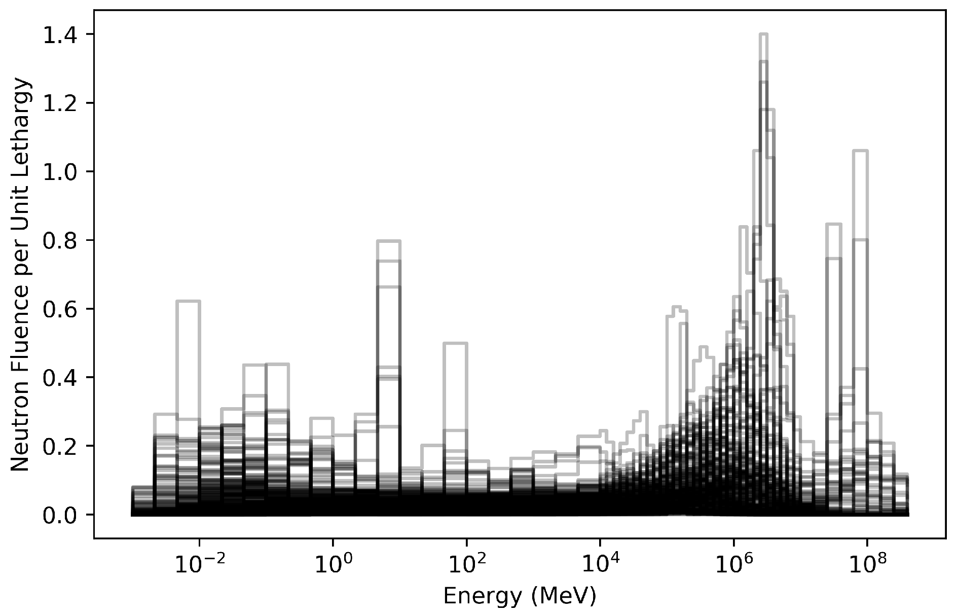
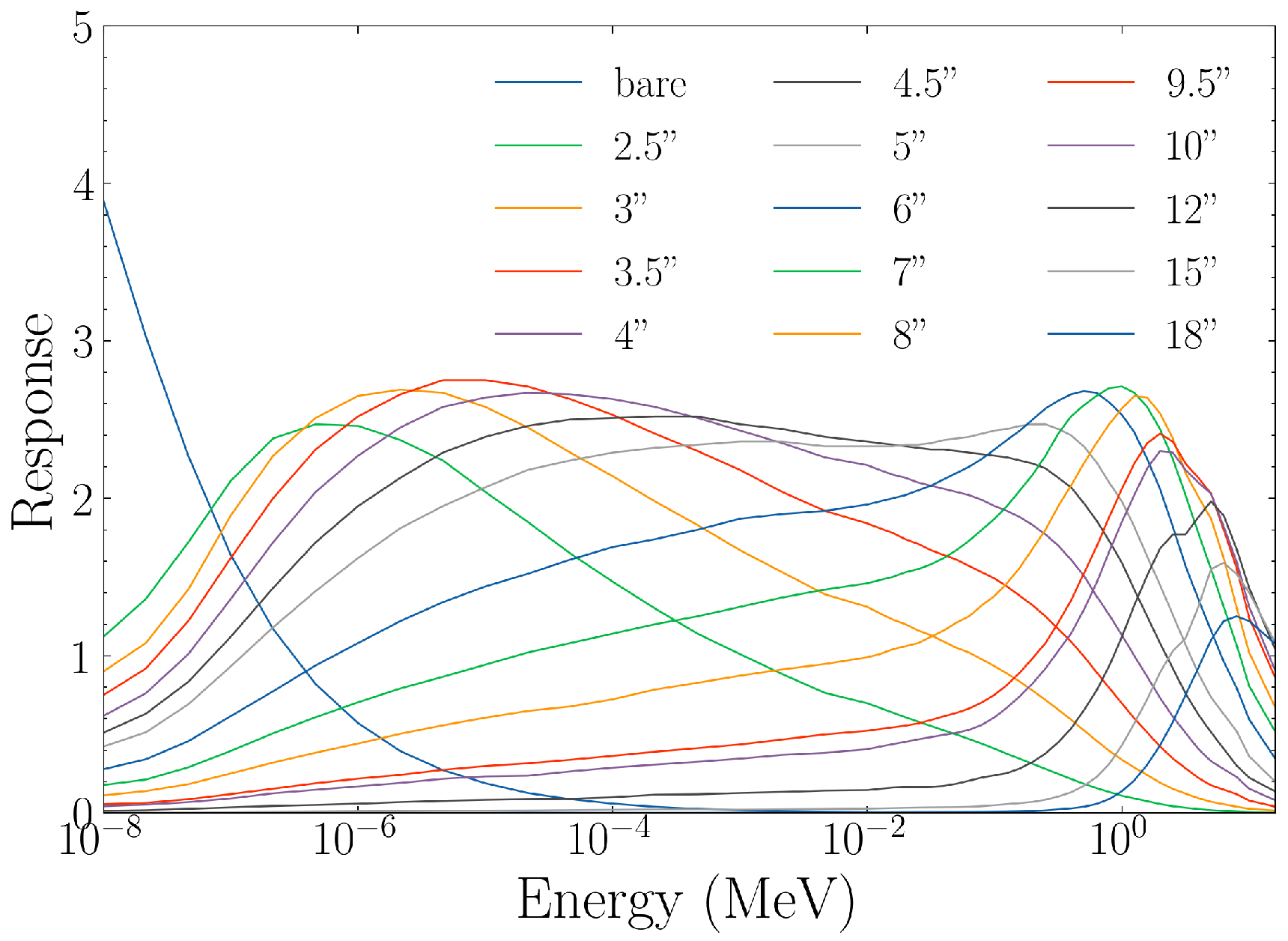
To evaluate the effectiveness of a neutron energy spectra generation algorithm, a data set of real-world neutron energy spectra was needed on which to test unfolding performance. For this work, we used an IAEA technical report [8] containing 251 measured and simulated neutron energy spectra which range from eV to MeV. All 251 spectra are plotted in Figure 1, and the kinds of spectra present in this set are shown in Table 1. These spectra cover a wide range of applications that include calibration sources, evaporation fields, cosmic ray background, and reactor spectra. Our neural networks seek optimal performance on this wide variety of spectra, but we believe these methods would be applicable to constrained neutron energy ranges as well. This report also contains a fully solved Bonner sphere detector response matrix (Figure 2), with which we may calculate an expected detector response given any discretized neutron energy spectrum:
Here, is the expected response of the ith Bonner sphere; R is the detector response matrix, which characterizes the response of the ith Bonner sphere to neutrons in the jth energy bin ; and is the neutron energy spectrum. Neutron energy spectra are always normalized to unity:
Figure 1.
All 251 real-world neutron energy spectra provided by the IAEA technical report [8] plotted on top of each other.
Figure 1.
All 251 real-world neutron energy spectra provided by the IAEA technical report [8] plotted on top of each other.

Figure 2.
The IAEA Bonner sphere response function for 15 different moderator thicknesses (in inches).
Figure 2.
The IAEA Bonner sphere response function for 15 different moderator thicknesses (in inches).


Table 1.
The kinds of neutron energy spectra present in the IAEA data set are shown in column 1. The number of spectra for each kind is shown in column 2, and the number of spectra present in the 62 IAEA spectra designated for use by the PSA algorithm (Section 2.2.1) is shown in column 3.
Table 1.
The kinds of neutron energy spectra present in the IAEA data set are shown in column 1. The number of spectra for each kind is shown in column 2, and the number of spectra present in the 62 IAEA spectra designated for use by the PSA algorithm (Section 2.2.1) is shown in column 3.
| Spectra Kind | Number Present | Number Used by PSA |
|---|---|---|
| reference | 11 | 2 |
| moderated reference | 13 | 4 |
| fission | 102 | 30 |
| moderated fission | 12 | 4 |
| workplace | 27 | 6 |
| fusion | 4 | 1 |
| high energy | 17 | 4 |
| accelerator | 47 | 7 |
| cosmic ray | 5 | 1 |
| boron therapy | 13 | 3 |
2.1. Unfolding Neural Network Architecture
For this paper, the unfolding neural network used is a densely-connected network with two hidden layers. Both hidden layers use the leaky rectified linear unit (Leaky ReLU) activation function, and the final layer uses a linear activation function. Leaky ReLU was chosen over other activation functions such as sigmoid and ReLU, as we found that Leaky ReLU hidden layers yielded the smallest mean squared and mean absolute unfolding errors for this specific unfolding problem. Dropout layers are placed between every pair of densely connected layers in the hope that they will prevent over-fitting and improve unfolding generalizability [15].
The tunable hyper-parameters of the network include the training batch size, the slope of the Leaky ReLU activation function, the neuron dropout rate, and the number of neurons in each hidden layer. Optimal hyper-parameters were determined through Bayesian hyper-parameter tuning [16]. This hyper-parameter tuning was performed against the IAEA spectra, however these hyper-parameters are used for all neural networks throughout this work regardless of the training data used. This was done to ensure consistency in the complexity of the unfolding network so that differences in unfolding performance may be primarily attributed to the quality of the training data. All networks will have identical architecture, but the weights and biases of each layer which are determined from back propagation depend entirely upon the training set used.
2.2. Random Neutron Spectra Generation Algorithms
2.2.1. Baseline Methods: Perturbed IAEA Spectra (PSA) and Random Spectra (RAND)
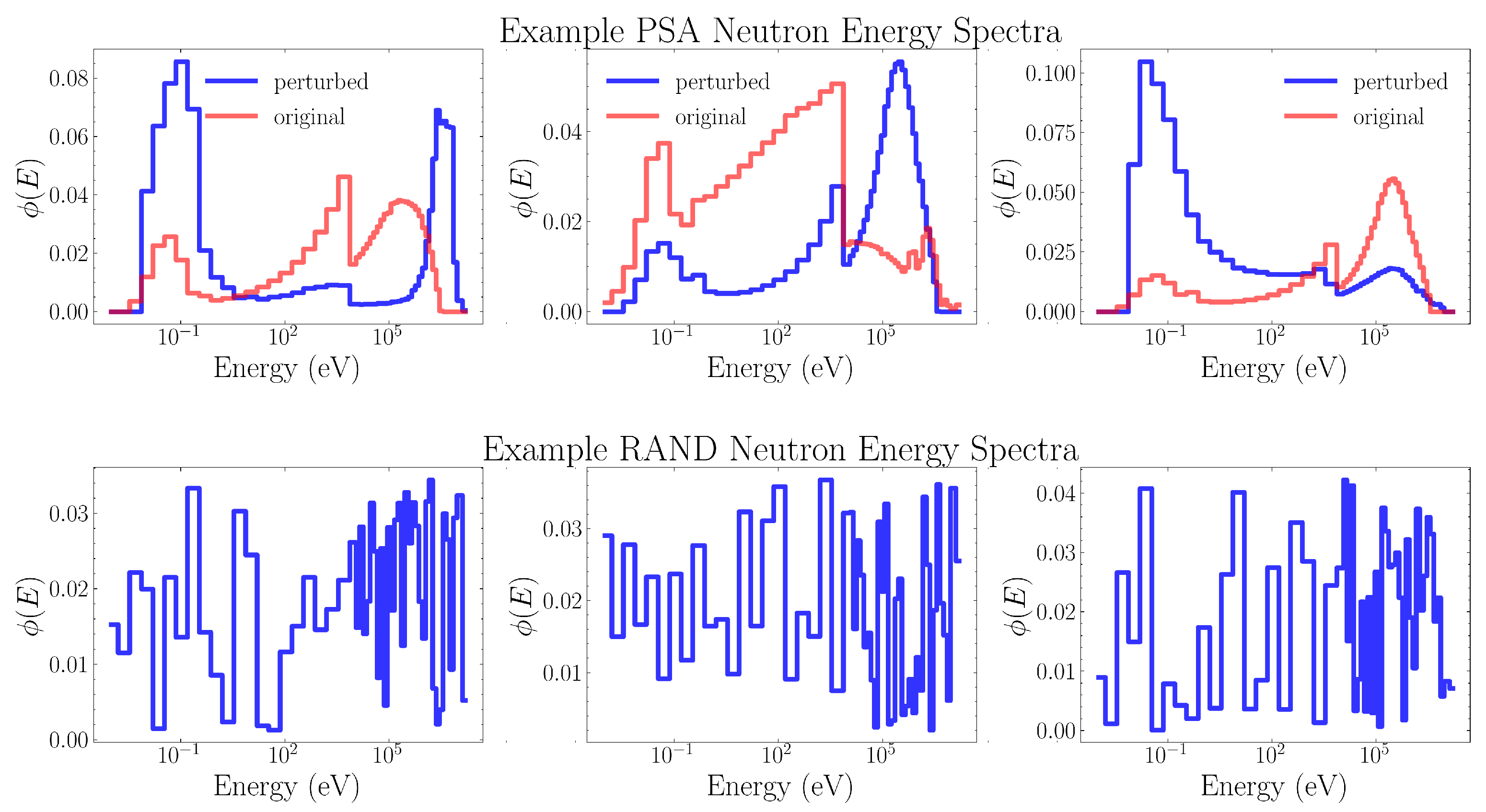
We select baseline neutron energy spectra generation algorithms in order to evaluate the effectiveness of our other spectra generation algorithms. The first algorithm uses random spectra (RAND) where each energy bin is given a random value between 0 and 1. Then, the entire spectrum is properly normalized according to Equation (2). Because this method places zero constraints on the types of neutron energy spectra our neural network will be exposed to during training it will be used as a baseline to evaluate the effectiveness of non-physical training data. Example random spectra are shown in Figure 3.
We would also like to be able to approximate a near-perfectly constrained solution space. While we could train directly on IAEA spectra, the 251 spectra contained in the IAEA report are not enough to effectively train an unfolding network on—we were unable to get performance comparable to our other unfolding networks using a 80-20 training-validation split of only IAEA spectra. Instead, perturbations were performed on a random subset of of the 251 IAEA spectra—this technique will be referred to as the perturbed spectra algorithm (PSA). This was done so that the remaining of the IAEA spectra may be quarantined and used only for final analysis. Since this method is only capable of producing neutron energy spectra which closely resemble the IAEA data, a neural network trained on this algorithm would likely not generalize as well to neutron energy spectra which are not already present in the IAEA data set. This algorithm is also highly specific to the exact energy bin structure used by the IAEA report. Therefore, it is used only as an upper-bound baseline for training data specificity, against which we may compare other neutron spectra generation algorithms.
For the PSA algorithm, one spectrum is randomly selected from the 62 IAEA spectra which were previously designated for use (listed in Table 1). In addition, a scaling factor is chosen from a normal distribution, with a mean 1 and a width of :
The chosen spectrum is interpolated, and this scaling factor is used to create a new neutron energy spectrum:
After this perturbation, the spectrum is properly normalized (Equation (2)). This algorithm has a single tunable feature parameter which will be optimized using the method outlined in Section 2.3.2. Example perturbed spectra are shown in Figure 3.
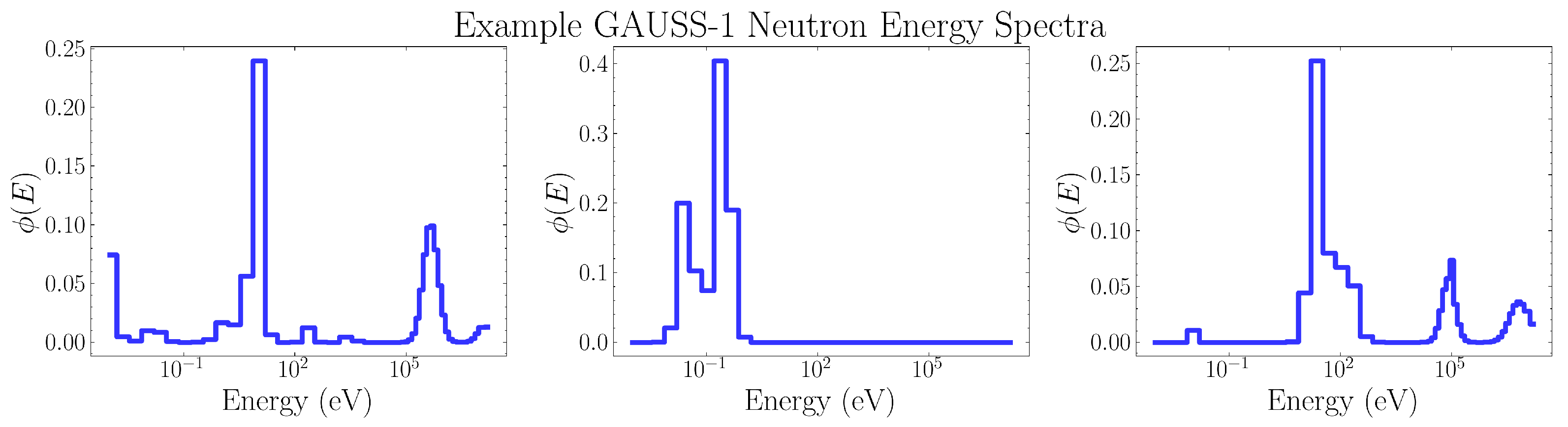
2.2.2. Method 1: GAUSS1
This algorithm relies on the qualitative observation that most real-world neutron energy spectra, when viewed on a logarithmic energy scale, consist primarily of one or more overlapping peaks. At greater than 1 MeV energies, neutrons resulting from fission or evaporation may show up as distinct peaks in the energy distribution. At thermal neutron energies of less than 1 eV, these structures are generally smaller in amplitude and result from thermalization physics. As a rough approximation to the shape of these peaks when viewed on a logarithmic scale, Gaussians were chosen due to their mathematical simplicity and smoothness.
This spectrum generation algorithm works by adding a random number of Gaussian peaks to a blank neutron energy spectrum. The process is controlled by several tunable parameters:
- —parameters between 0 and 1, which correspond to the mean and standard deviation of the normal distribution of means of the Gaussian peaks.
- —parameters between 0 and 1, which correspond to the mean and standard deviation of the normal distribution of widths of the Gaussian peaks.
- —controls the amount by which to cumulatively suppress the amplitude of subsequent Gaussian peaks. In general, this gives rise to one central energy peak, surrounded by smaller amplitude structures.
- —controls random deviations of the amplitude of the Gaussian.
- —the probability to add an extra Gaussian peak to the spectra.
These are the feature parameters of the spectra generation algorithm, and must be tuned to reasonable values by comparison to the IAEA neutron energy spectra. Processes for tuning each of these parameters is outlined in Section 2.3.
To generate a neutron energy spectrum we begin with a blank spectrum in which all energy bins are initialized to zero. Then, an iterative process is carried out in which one or more Gaussian-shaped peaks are added on top of this blank spectrum. Starting with ,
- 1.
- Parameters for the width and position of the Gaussian peak, on a logarithmic scale, are sampled from their corresponding normal distributions. The values and 10 correspond to the logarithms of the lowest energy bin value and the number of orders of magnitude which our energy bins cover ( eV to eV), respectively.
- 2.
- The mean height is perturbed according to :
- 3.
- A logarithmic Gaussian is added to the neutron energy bins:
- 4.
- The mean amplitude for the next iteration is suppressed according to :
- 5.
- and this entire process is repeated with a probability of
2.2.3. Method 2: GAUSS2
This algorithm is very similar to method 1; however, it further constrains the types of possible neutron energy spectra by coupling the width and height of the Gaussian peaks to their central energy. This is based on the observation that, due to the physics of neutron thermalization, Gaussian structures at lower energies tend to have smaller amplitudes. Structures with a larger energy spread will also tend to have smaller amplitudes than those which are highly concentrated around some central energy.
The tunable parameters for this algorithm are:
- —parameters between 0 and 1, which control the statistics of the width of the Gaussian peaks.
- —controls how strongly a Gaussian peak’s width is suppressed by its energy scale.
- —controls how strongly a Gaussian peak’s amplitude is increased by its energy scale.
- —controls the amount by which to cumulatively suppress the amplitude of subsequent Gaussian peaks.
- —the probability to add an extra Gaussian peak to the energy spectra.
Similarly to method 1, these feature parameters must be tuned to reasonable values prior to usage (Section 2.3).
To generate a neutron energy spectrum, we will once again start with a blank spectrum in which all energy bins are initialized to zero. Then, the following iterative process is carried out, starting with ,
- 1.
- A value between 0 and 1 is randomly chosen:
- 2.
- Parameters for the width and position of the Gaussian peak, as seen on a logarithmic scale, are determined:
- 3.
- The amplitude of the Gaussian is suppressed according to :
- 4.
- The Gaussian is added to the logarithm of the neutron energy bins:
- 5.
- The amplitude for the next iteration is suppressed according to :
- 6.
- and this entire process is repeated with a probability .
2.2.4. Method 3: FRUIT Spectra Generation Algorithm
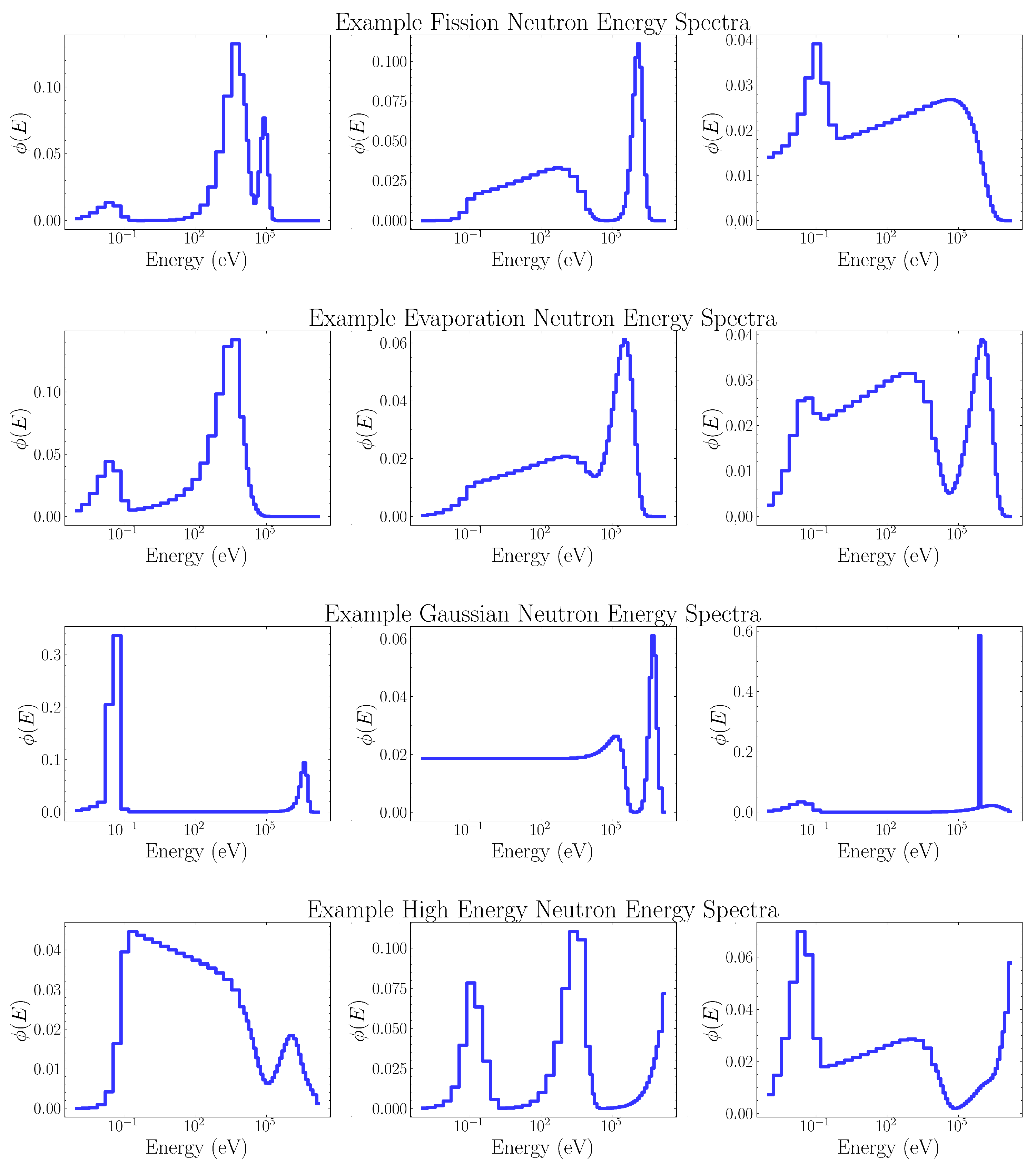
This spectrum generation algorithm is inspired by the Frascati Unfolding Interactive Tool (FRUIT) [12]. FRUIT iteratively unfolds neutron energy spectra by assuming that they are well described by one of four theoretical models: fission, evaporation, Gaussian, or high energy spectra. These four models describe a wide variety of common neutron energy spectra, including fission sources, radionuclide neutron sources, medical cyclotrons, and hadron accelerators [12].
The fission, evaporation, Gaussian, and high energy models consist of a weighted sum of four component spectra, describing the physics of thermal, epithermal, fast, and high energy neutrons. The component spectra for each model have been reprinted in Table 2. Importantly for this paper, each of these component spectra takes tunable parameters. By properly selecting well motivated parameters, we generate physically accurate spectra for the given model type. The tunable parameters for each model are:
- Fission:
- Evaporation:
- Gaussian:
- High Energy:
Table 2.
The thermal, epithermal, fast, and high energy component spectra for each of the four FRUIT models [12]. Note the inconsistent units across each component spectra—this problem is remedied through proper normalization, which is done before the weighted sum of each component is performed.
Table 2.
The thermal, epithermal, fast, and high energy component spectra for each of the four FRUIT models [12]. Note the inconsistent units across each component spectra—this problem is remedied through proper normalization, which is done before the weighted sum of each component is performed.
| Model | Thermal | Epithermal | Fast | High Energy |
|---|---|---|---|---|
| Fission | 0 | |||
| Evaporation | ↓ | ↓ | 0 | |
| Gaussian | ↓ | ↓ | 0 | |
| High Energy | ↓ | ↓ |
Bedogni et al. [12] interpret each parameter taken by these models, and provide definite values for MeV, the conventional thermal neutron energy, and MeV, the lower energy range of epithermal neutrons. The parameters , , , and control the proportion of each model’s spectrum that comes from the thermal, epithermal, fast, and high energy components, respectively.
To randomly generate neutron energy spectra from these models, we must first determine reasonable distributions for each model parameter. To do this the fission, Gaussian, and high energy models were fitted to each individual IAEA neutron energy spectrum. Since the high energy model is identical to the evaporation model but with extra degrees of freedom from the high energy component, the evaporation model was not considered for fitting; the high energy model is always guaranteed to provide an equivalent or better fit. Due to the high degree of non-linearity within each model’s fitting parameters, the accuracy of the fit depends heavily upon the initial guesses for the fit parameters. To find a globally optimal fit, Bayesian optimization was used to search for appropriate initial guesses. For each IAEA spectrum, only the model that had the minimal mean squared fitting error was considered.
Using these distributions for each model parameter, which should cover the possible values taken by realistic neutron energy spectra, the procedure of generating a random neutron energy spectra is as follows:
- 1.
- Randomly select between the fission, evaporation, Gaussian, or high energy models.
- 2.
- Randomly sample model parameters from the distributions determined from IAEA spectra. For an evaporation spectrum, parameters are sampled from the relevant high energy parameter distributions.
- are always selected from the same fit so that they sum to 1, ensuring normalization.
- 3.
- Create the final spectrum as a weighted sum of the relevant component spectra:
Example spectra for each model type are shown in Figure 6 below.
2.3. Tuning the Feature Parameters of a Spectra Generation Algorithm
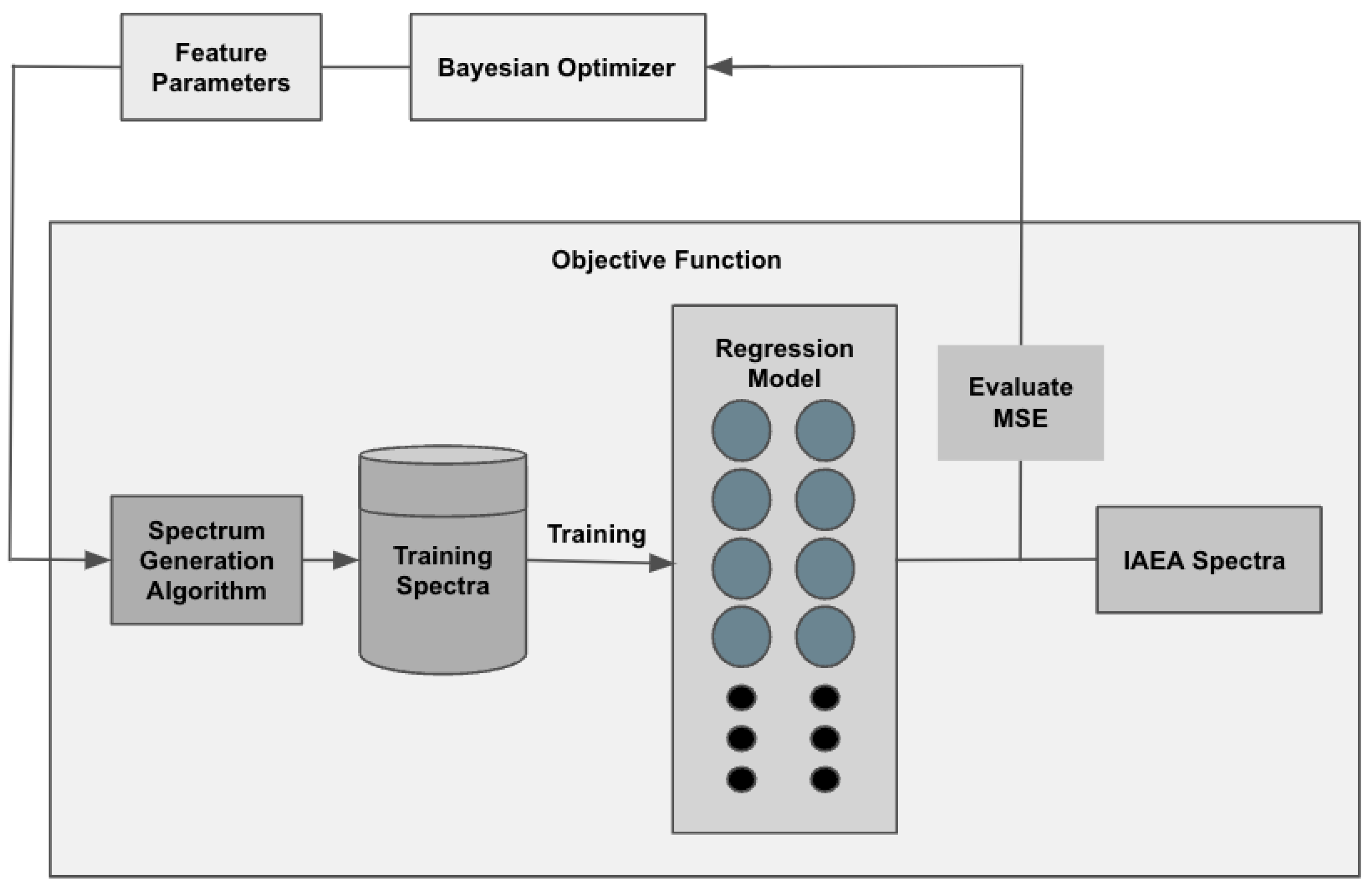
The PSA, GAUSS-1, and GAUSS-2 algorithms all take one or more feature parameters which must be tuned in order to maximize the unfolding performance of a neural network trained on the produced spectra. To evaluate the effectiveness of a given choice of feature parameters, we must first construct an objective function to optimize against. This objective function should take a given set of feature parameters and return the effectiveness of those feature parameters at generating realistic spectra. In particular, we would like our objective function to capture the idea that neural networks which have been trained on data from a properly tuned algorithm will have the best possible unfolding performance when shown real-world neutron energy spectra. This feature parameter tuning process is outlined in Figure 7. We consider two candidate objective functions.
2.3.1. Feature Parameter Tuning by Evaluation on Neural Networks
The first objective function takes a brute force approach; the feature parameters are used to create a training set which is then used to train an unfolding neural network. This is done four times, to create four separate unfolding networks trained on four distinct sets of randomly generated neutron energy spectra with the same feature parameters. The cost function returns the average mean squared error unfolding performance of these four networks when evaluated on IAEA neutron energy spectra.
2.3.2. Feature Parameter Tuning by Evaluation on Linear Regression Models
For the second objective function, the unfolding neural network is replaced with a linear regression model,
where is a matrix which maps the jth detector response bin to the ith energy bin in a neutron energy spectra.
Although far simpler than a neural network, linear regression models still involve a training step in which the model weights are tuned to minimize unfolding error against a training set. We do not expect a linear regression model to perform as well as an unfolding network, however both types of regression will still benefit from a properly constrained solution space—just like a neural network, a linear regression model which has been trained on realistic neutron energy spectra will far outperform one which has been trained on purely random data when unfolding real-world spectra.
The second objective function evaluates the effectiveness of a given set of feature parameters by training four linear regression models on four distinct sets of neutron energy spectra, randomly generated from the given feature parameters. The objective function then returns the mean squared unfolding error of each linear regression model when evaluated on the IAEA data set.
3. Results
When attempting to evaluate the effectiveness of a spectrum generation algorithm for the purposes of training an unfolding neural network, there is a great deal of inherent uncertainty. This uncertainty comes primarily from the randomly initialized neuron weights and biases, which can lead two separate networks trained on identical data to find two completely different loss function minima. In order to account for this uncertainty when evaluating a given spectra generation algorithm, an ensemble of thirty networks with identical architecture is trained on the same 3000 randomly generated spectra. Analysis of mean squared unfolding error and mean absolute unfolding error is performed on individual neural networks and then averaged across the thirty distinct networks.
3.1. Optimal Feature Parameters for PSA, GAUSS-1, and GAUSS-2
The feature parameters of GAUSS-1 and GAUSS-2 were tuned by means of Bayesian optimization, with the neural network and linear regression objective functions both utilized. All objective function optimizations were performed over the same computation time. When compared to the neural network objective function, Bayesian optimization performed on the linear regression objective function was able to search much more of the parameter space since evaluations of its objective function were dramatically quicker. This yielded two separate optimal feature parameters, according to each objective function. Table 3 shows the average unfolding performance for networks trained on the GAUSS-1 and GAUSS-2 algorithms, for both sets of optimal feature parameters, when evaluated on IAEA spectra.
For both GAUSS-1 and GAUSS-2 the feature parameters found through optimization of the linear regression objective function gave better unfolding performance, when training a neural network to unfold IAEA spectra, compared to the feature parameters found through optimization of the neural network objective function. For the rest of our analysis, unless otherwise specified the feature parameters found through linear regression will be used due to their superior performance.
3.2. Unfolding Performance of Each Algorithm
Table 4 shows the average mean squared and mean absolute unfolding error for networks trained on each of the five spectra generation algorithms, when evaluated on IAEA spectra.
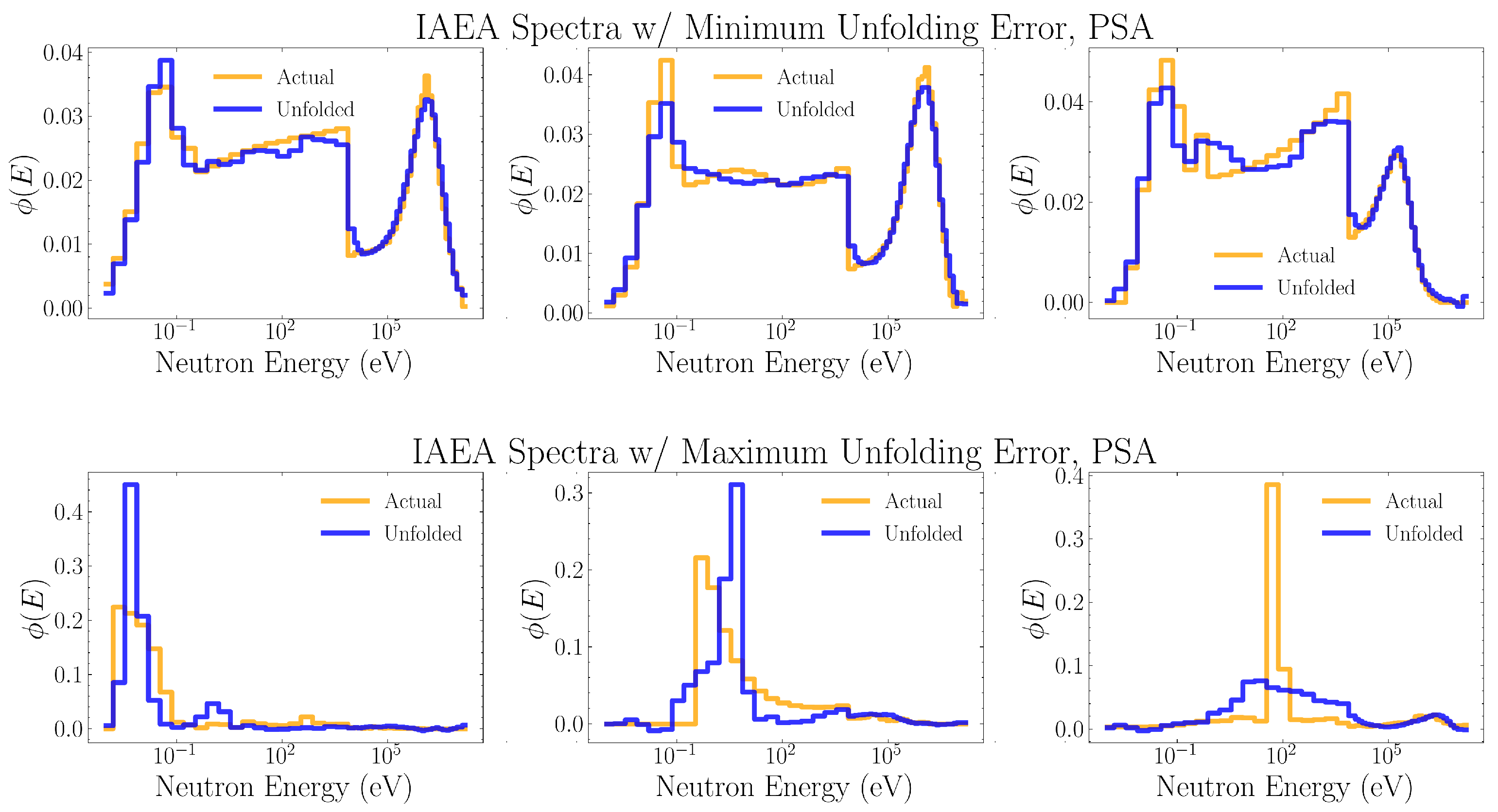
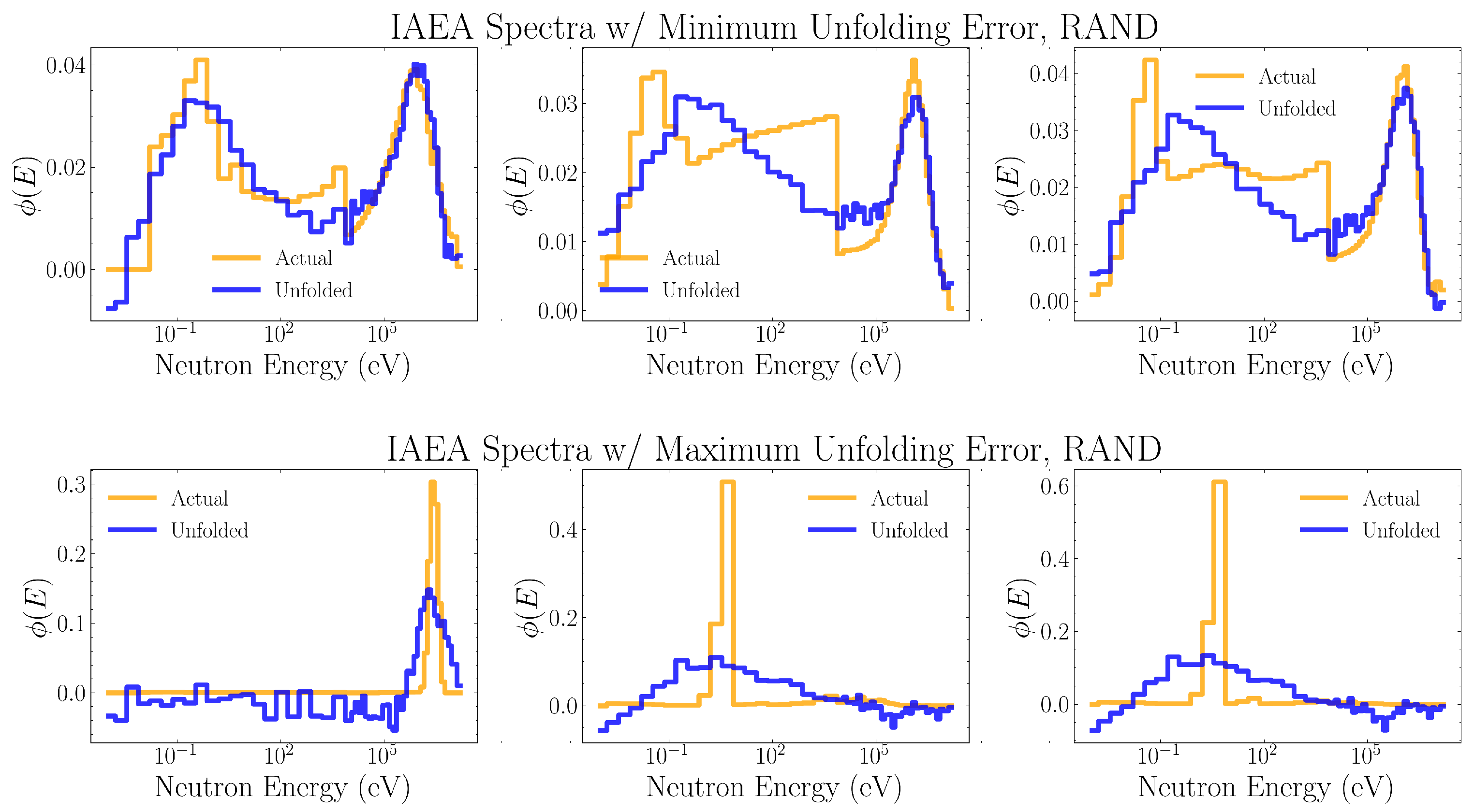
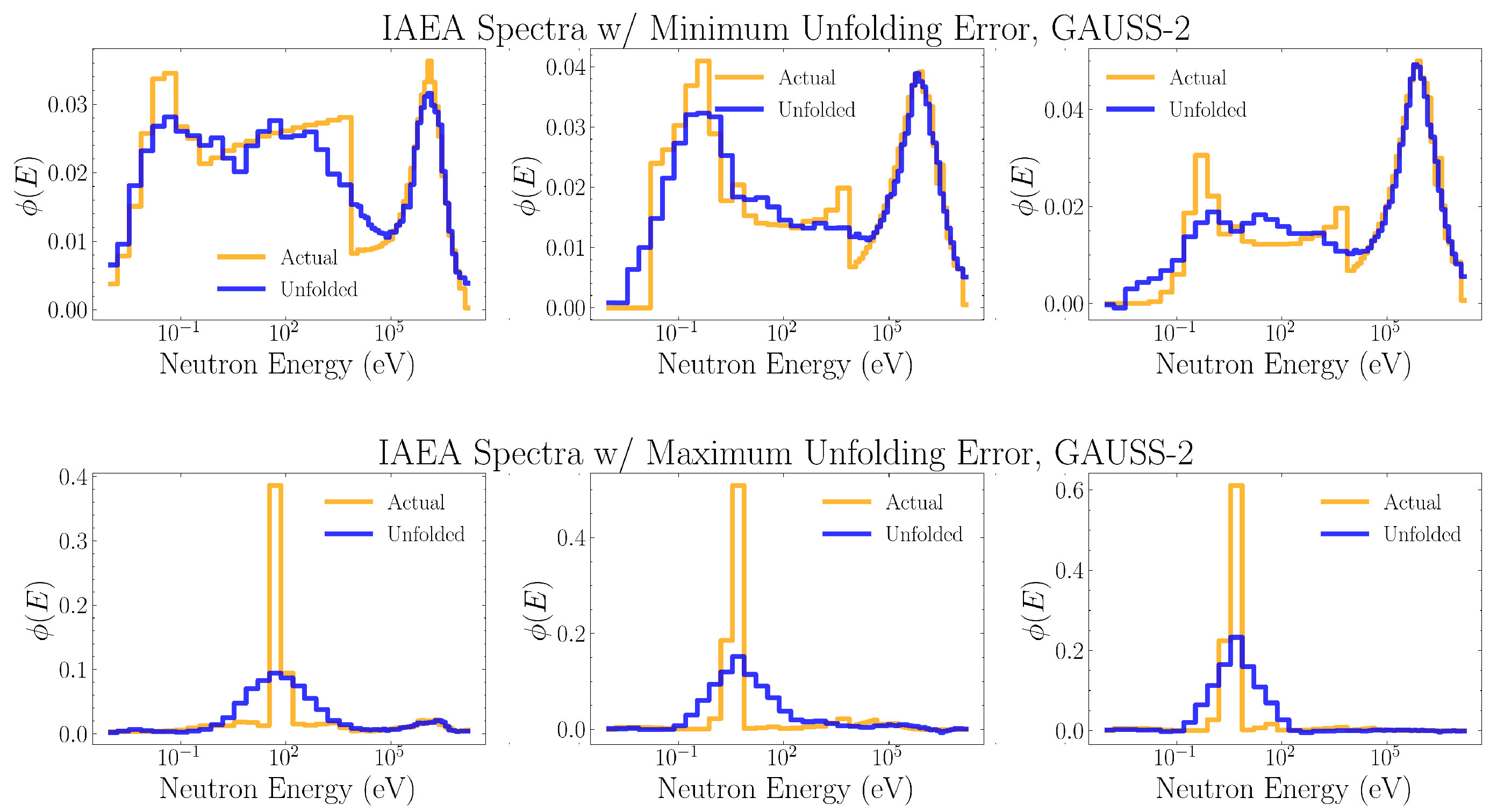
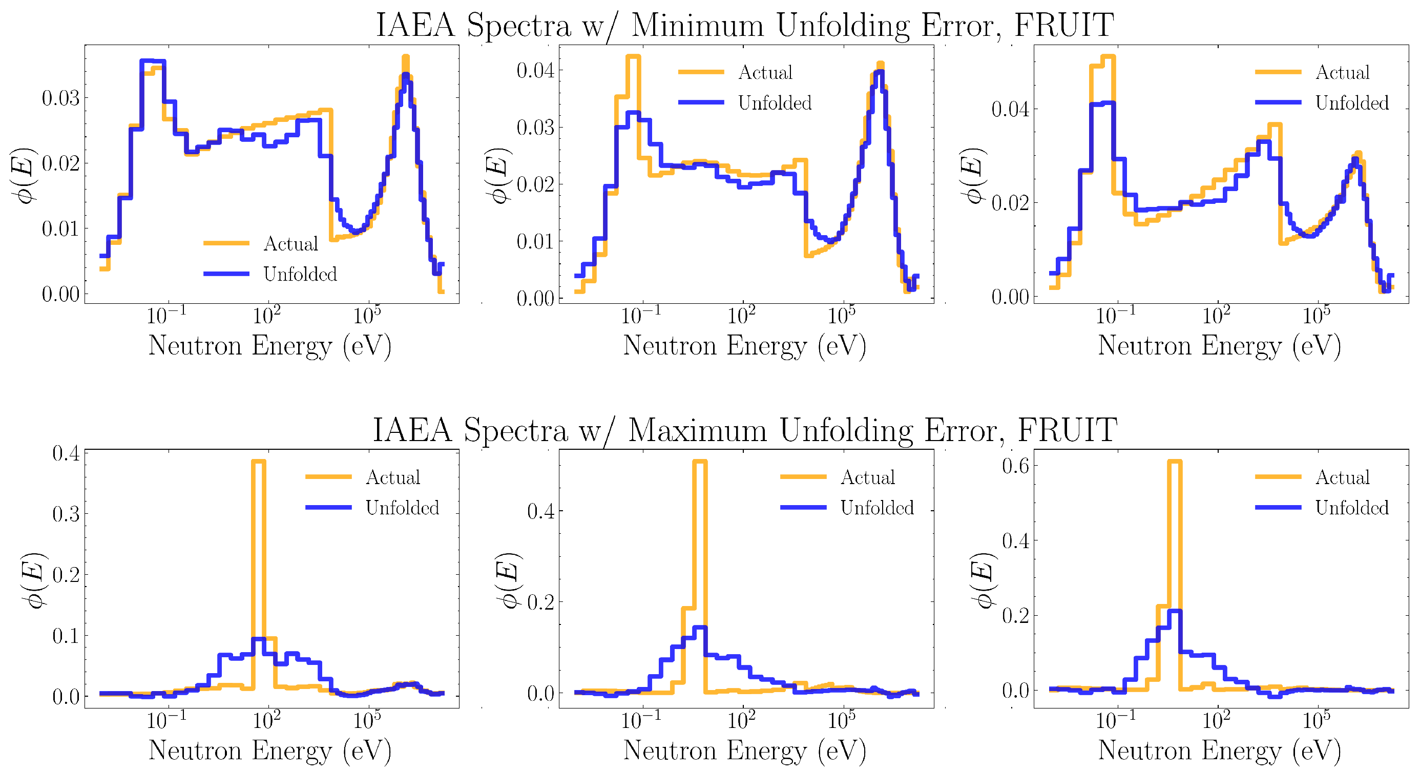
Figure 8, Figure 9, Figure 10, Figure 11 and Figure 12 show the three IAEA spectra which were unfolded with the least MSE and the three IAEA spectra which were unfolded with the most MSE, for neural networks trained on the the PSA, RAND, GAUSS-1, GAUSS-2, and FRUIT algorithms, respectively.
The IAEA neutron energy spectra set contains several kinds of commonly encountered neutron sources, such as fission, fusion, high energy, etc. Some of these sources also include moderators, giving rise to lower energy thermalized neutrons. Figure 13 shows the mean squared unfolding error of Table 4, sorted according to the kind of spectra being unfolded.
3.3. Unfolding Accuracy for Radiation Dosimetry
For some applications, such as radiation dosimetry, the precise shape of the unfolded spectra is not the primary objective. Although an unfolded spectrum might oscillate around the true neutron energy spectrum, when this spectrum is convoluted with equivalent dose weighting factors these oscillations may average out yielding an accurate dose estimate. To perform this analysis, neutron group fluence to ambient dose equivalent coefficients provided by the IAEA technical report [8] were used. The calculated dose equivalent is the dose equivalent in soft tissue at a depth of 10 mm. The neutron group fluence for a given neutron energy spectrum bin is calculated according to
The ambient dose equivalent is then calculated as
where n is a scaling factor which depends upon the emission rate of the neutron source. For analysis only the percent error in dose is considered, and so n does not affect the results.
Table 5 shows the percent error between the dose calculated by the unfolded spectra and the dose calculated using the known neutron energy spectra. The average and standard deviation in percent dose error across all IAEA spectra for a given unfolding network is calculated and then this value is averaged over all thirty networks.
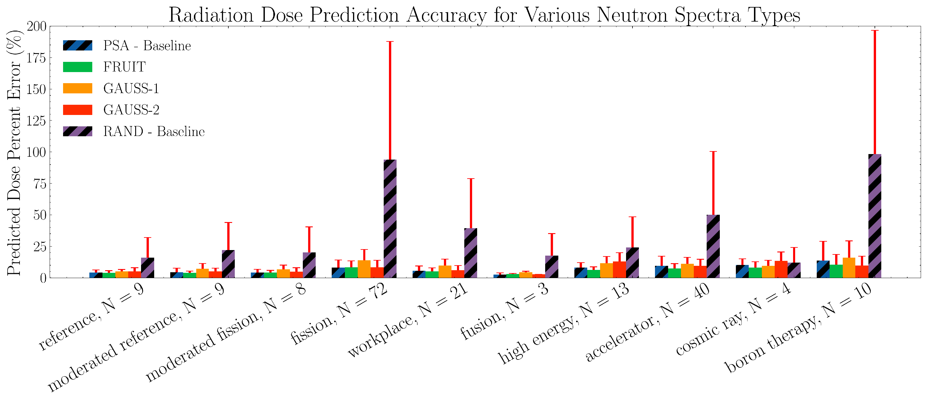
Figure 14 shows the mean percent error in dose prediction, sorted according to the kind of spectra being unfolded.
4. Discussion
The results shown in Table 3 demonstrate that linear regression models may be used as an effective proxy when performing feature engineering on the training data of a neural network. Although a neural network based objective function will provide the most accurate metric of expected unfolding performance, it will also be extremely computationally expensive. Each objective function evaluation will involve fully training multiple unfolding networks, in order to account for deviations between networks, which can take several minutes. Since an objective function is called several hundred times or more while searching for a minimum, this will prevent any optimization algorithm from performing an extensive search across the parameter space in a reasonable time frame. The linear regression objective function sacrifices accuracy in calculating expected mean squared unfolding error in order to dramatically reduce computational complexity. This allows optimization algorithms such as Bayesian optimization to perform a much wider search over the parameter space.
Although the kinds of neural networks used for unfolding and the specific architecture of those networks vary widely throughout the literature, this work was performed in the hope that our optimal training spectra would remain optimal across a wide range of regression models. There are several properties, such as the hyper-parameters of an unfolding network, which are highly specific to the exact neural network architecture being employed. However, the fact that the optimal feature parameters for a linear regression model remained optimal when being used to train a neural network provides context to the potential for the same spectra generation algorithms outlined in this work to be employed across a wide variety of network architectures. When unfolding onto a different energy bin structure we are less confident that these spectra generation algorithms will be optimal. This is why procedures for feature parameter tuning have been discussed—so that this work may be reproduced for other energy ranges and resolutions of interest.
In Table 4, we can see that the PSA-trained networks and the RAND-trained networks had the least and greatest mean squared and mean absolute unfolding errors, respectively. This is not surprising, as these algorithms were intended as upper and lower bounds on the degree of solution space constraint. On average the mean squared unfolding error of the PSA-trained networks, with their properly constrained training domains, were more than three times less than the RAND-trained networks. The mean absolute unfolding error of the PSA-trained networks was about two and a half times less than the RAND-trained networks. In addition, when using these unfolded networks for dosimetry purposes (Table 5), the RAND-trained networks gave dose estimates with more than 7 times as much error as the PSA-trained networks. This provides a rough sense of scale to the difference in unfolding performance expected between a network trained on physical vs. non-physical spectra.
It is important to note, however, that mean squared error and mean absolute error are flawed metrics for evaluating unfolding performance which under-represent how much more valuable the PSA-unfolded spectra would be when used for dosimetry or source characterization. This is illustrated when comparing the best-case and worst-case PSA-trained unfolding (Figure 8) to that of the RAND-trained unfolding (Figure 9). We can see that RAND-trained networks were incapable of confidently unfolding important qualitative features of the energy spectra. If these unfolded spectra were to be used for source characterization, even the best-case unfolding would be unable to correctly identify the radiation source. On the other hand, the worst-case unfoldings for the PSA-trained networks were still able to identify the rough shape and energy scale of structures within the spectra. Although the average mean squared unfolding error of networks trained on these upper and lower bound baselines of training domain constraint differ by only a factor of three, within the context of unfolding use cases a properly constrained training domain can mean the difference between highly accurate or entirely useless unfolding.
Table 4 also shows that the GAUSS-2-trained networks had 20% less mean squared unfolding error on average than the GAUSS-1-trained networks. This difference in performance may also be seen in Table 5, where GAUSS-2-trained networks predicted doses with 30% less mean percent dose error than GAUSS-1-trained networks. This trend is likely due to the heavier constraints which the GAUSS-2 algorithm places on the training domain through coupling the width and height of the added Gaussian peaks to the magnitude of their central energy. This means that lower energy Gaussian peaks will be smaller in amplitude and broader in width, resembling the physics of thermalized neutrons. In particular, we expected that this would translate into better unfolding performance of GAUSS-2-trained networks on moderated sources or spectra with more thermal neutrons present. This is partially demonstrated in Figure 13 and Figure 14, where the GAUSS-2-trained networks have less mean squared unfolding error and percent dose error than the GAUSS-1-trained networks when evaluated on fission, moderated fission, and moderated reference spectra. On the other hand, GAUSS-2-trained networks see a decrease in unfolding performance compared to GAUSS-1-trained networks for spectra with no thermalization such as high energy and cosmic ray. The dosage predictions for these spectra types from GAUSS-2-trained networks are worse than those from GAUSS-1-trained networks, and occasionally worse than RAND-trained networks. This difference in performance is likely because the GAUSS-2 algorithm attempts to enforce low-energy neutron thermalization, thus poorly representing any non-thermal low energy structures. However, these differences in unfolding performance are not dramatic.
Out of the three spectra generation algorithms to be investigated, the unfolding neural networks trained on FRUIT data performed the best, on aggregate, in both mean squared unfolding error (Table 4) and dosage estimation (Table 5). In fact, the dosage estimates of the FRUIT-trained networks were more accurate on average than the estimates made by PSA-trained networks, even though PSA was intended to be an upper-bound on performance. Since the FRUIT algorithm generates spectra from one of four theoretical models—fission, evaporation, high energy, and Gaussian—we would expect networks trained on it to perform particularly well when unfolding real spectra of these categories. On the other hand, FRUIT-trained networks should not perform nearly as well when unfolding accelerator, cosmic ray, or medical spectra as these are not modeled for by the algorithm. However, this trend is not seen in Figure 13 or Figure 14, and the FRUIT-trained networks seem to be capable of generalizing to many types of neutron spectra.
Certain trends in the mean squared unfolding error across spectra types align with what we would anticipate from the design of each spectra generation algorithm. However, there are no spectra types for which the mean squared unfolding error of networks trained on a specific algorithm clearly stands out. Instead, it seems that there are particular kinds of spectra which are generally easier to unfold with a lower mean squared error. Looking at Figure 8, Figure 9, Figure 10, Figure 11 and Figure 12, unfolding mean squared error was universally lower for spectra which consisted of a single peak. Due to the normalization constraint, these single-peaked spectra necessarily have an extremely high amplitude. If the unfolding networks do not match the small number of large amplitude bins, even if they are correct about the rough energy range, the MSE will be very large due to the squaring of the residuals. On the other hand, a large number of small discrepancies within spectra consisting of multiple structures, such as for the best-case unfolding of RAND-trained networks (Figure 9), will contribute much less to the MSE even if the quality of the unfolding is very poor. These problems can be improved by considering other loss functions, such as mean absolute error, which do not penalize outliers as heavily. For this reason, the mean absolute unfolding error has been included in Table 3 and Table 4. However, due to the wide-spread use of MSE as a metric for spectrum unfolding, and to facilitate easy comparison of our unfolding performance to other works, we have chosen to primarily use MSE in our analysis.
5. Conclusions
In this paper, we presented three methods for the random generation of large quantities of realistic and physically motivated neutron energy spectra, without the need for expensive experiment or Monte-Carlo simulations. This work was based on the observation that, regardless of the specifics of an unfolding network’s architecture, the performance and generalizability of any neural network based unfolding algorithm would be dramatically impacted by the quality and quantity of neutron energy spectra used to train it.
Our analysis was performed on 189 of the 251 IAEA neutron energy spectra (with the other 62 spectra being used by the PSA algorithm), which were quarantined during the training of the unfolding networks in order to prevent any data leakage. We demonstrated that these neutron energy spectra generation algorithms far outperformed random training data which were not physically motivated. Out of the three spectra generation algorithms investigated, neural networks trained on the FRUIT spectrum generation algorithm (Section 2.2.4) had the greatest overall unfolding performance on IAEA spectra. This is because it relied on theoretical models which are able to accurately capture the physics of fission, high energy, and evaporative spectra—all of which are present in large quantities in the IAEA data. We also determined that linear regression models could be used in proxy of an unfolding neural network to evaluate the performance of a particular set of training data.
A limitation of the results presented in this paper is the small number of validation spectra used in our analysis, as the 251 IAEA spectra do not encompass all possible types of neutron energy spectra found in the real-world. Although the general techniques outlined in this paper may be applied to the feature engineering stage of any future work on neural network based unfolding, the relative performance of each algorithm will depend upon the energy ranges of interest and the spectra types to be unfolded.
Future work could improve the generalizability of networks trained on FRUIT spectra by constructing more theoretical models for a wider range of spectra types and by performing further analysis on how to optimally select parameters for each model. Future work could also investigate other metrics of unfolding performance which address the problems with MSE discussed in this paper. For example, to optimize for dosage prediction accuracy, the percent error in predicted ambient dose equivalent could be embedded into the loss function used for training or the objective function used for feature parameter tuning (Section 2.3).
All code and relevant analysis have been made publicly available. Our hope for this work is that any project investigating neural network based neutron spectrum unfolding, regardless of the neural network architecture or kind of detector used, will be able to insert similar algorithms into the training data generation step in order to achieve optimal unfolding performance on the problem under investigation.
Author Contributions
Conceptualization, J.M., J.J.M. and D.S.; Data curation, D.S.; Formal analysis, J.M.; Investigation, J.M., J.J.M. and D.S.; Methodology, J.M., J.J.M. and D.S.; Software, J.M. and D.S.; Supervision, J.J.M. and D.S.; Visualization, J.M.; Writing—original draft, J.M.; Writing—review & editing, J.M., J.J.M. and D.S. All authors have read and agreed to the published version of the manuscript.
Funding
This material is based upon work supported in part by the Department of Energy National Nuclear Security Administration through the Nuclear Science and Security Consortium under Award Numbers DE-NA0003180 and DE-NA0003996. This material has been approved for release by LLNL under document number LLNL-JRNL-842794.
Institutional Review Board Statement
Not applicable.
Informed Consent Statement
Not applicable.
Data Availability Statement
The relevant code may be found at https://github.com/JamesMcGreivy/NeutronSpectraGeneration, accessed on 31 December 2022.
Conflicts of Interest
The authors declare no conflict of interest. The funders had no role in the design of the study; in the collection, analyses, or interpretation of data; in the writing of the manuscript; or in the decision to publish the results.
Abbreviations
The following abbreviations are used in this manuscript:
| IAEA | The International Atomic Energy Agency |
| MSE | The Mean Squared Error Loss Function |
| MAE | The Mean Absolute Error Loss Function |
References
- Glodo, J.; Wang, Y.; Shawgo, R.; Brecher, C.; Hawrami, R.H.; Tower, J.; Shah, K.S. New Developments in Scintillators for Security Applications. Phys. Procedia 2017, 90, 285–290. [Google Scholar] [CrossRef]
- Stange, S.; Esch, E.I.; Burgett, E.A.; Del Sesto, R.E.; Muenchausen, R.E.; Taw, F.L.; Tovesson, F.K. A fissionable scintillator for neutron flux monitoring. In Proceedings of the Penetrating Radiation Systems and Applications XII, San Diego, CA, USA, 21–24 August 2011; Grim, G.P., Schirato, R.C., Eds.; SPIE: Bellingham, WA, USA, 2011. [Google Scholar] [CrossRef]
- Mohammadi, N.; Hakimabad, H.M.; Motavalli, L.R. Neural network unfolding of neutron spectrum measured by gold foil-based Bonner Sphere. J. Radioanal. Nucl. Chem. 2014, 303, 1687–1693. [Google Scholar] [CrossRef]
- Ortiz-Rodriguez, J.M.; Reyes Alfaro, A.; Reyes Haro, A.; Solis Sanches, L.O.; Miranda, R.C.; Cervantes Viramontes, J.M.; Vega-Carrillo, H.R. Evaluating the performance of two neutron spectrum unfolding codes based on iterative procedures and artificial neural networks. AIP Conf. Proc. 2013, 1544, 114–121. [Google Scholar] [CrossRef]
- Sharghi Ido, A.; Bonyadi, M.; Etaati, G.; Shahriari, M. Unfolding the neutron spectrum of a ne213 scintillator using artificial neural networks. Appl. Radiat. Isot. 2009, 67, 1912–1918. [Google Scholar] [CrossRef] [PubMed]
- Kelley, R.P.; Rolison, L.M.; Lewis, J.M.; Murer, D.; Massey, T.N.; Enqvist, A.; Jordan, K.A. Neutron response function characterization of 4He scintillation detectors. Nucl. Instruments Methods Phys. Res. Sect. A Accel. Spectrometers Detect. Assoc. Equip. 2015, 793, 101–107. [Google Scholar] [CrossRef]
- Febbraro, M.; Becker, B.; deBoer, R.; Brandenburg, K.; Brune, C.; Chipps, K.; Danley, T.; Fulvio, A.D.; Jones-Alberty, Y.; Macon, K.; et al. Performance of neutron spectrum unfolding using deuterated liquid scintillator. Nucl. Instruments Methods Phys. Res. Sect. A Accel. Spectrometers Detect. Assoc. Equip. 2021, 989, 164824. [Google Scholar] [CrossRef]
- International Atomic Energy Agency. Compendium of Neutron Spectra and Detector Responses for Radiation Protection Purposes: Supplement to Technical Reports Series No. 318; International Atomic Energy Agency: Vienna, Austria, 2001. [Google Scholar]
- Bai, H.; Wang, Z.; Zhang, L.; Jiang, H.; Lu, Y.; Chen, J.; Zhang, G. Simulation of the neutron response matrix of an EJ309 liquid scintillator. Nucl. Instruments Methods Phys. Res. Sect. A Accel. Spectrometers Detect. Assoc. Equip. 2018, 886, 109–118. [Google Scholar] [CrossRef]
- Agostinelli, S.; Allison, J.; Amako, K.; Apostolakis, J.; Araujo, H.; Arce, P.; Asai, M.; Axen, D.; Banerjee, S.; Barrand, G.; et al. Geant4—A simulation toolkit. Nucl. Instruments Methods Phys. Res. Sect. A Accel. Spectrometers Detect. Assoc. Equip. 2003, 506, 250–303. [Google Scholar] [CrossRef] [Green Version]
- Goorley, J.T.; James, M.R.; Booth, T.E.; Brown, F.B.; Bull, J.S.; Cox, L.J.; Durkee, J.W., Jr.; Elson, J.S.; Fensin, M.L.; Forster, R.A., III; et al. Initial MCNP6 Release Overview—MCNP6 Version 1.0. Nucl. Technol. 2013, 180, 298–315. [Google Scholar] [CrossRef]
- Bedogni, R.; Domingo, C.; Esposito, A.; Fernández, F. Fruit: An operational tool for multisphere neutron spectrometry in workplaces. Nucl. Instruments Methods Phys. Res. Sect. A Accel. Spectrometers Detect. Assoc. Equip. 2007, 580, 1301–1309. [Google Scholar] [CrossRef]
- Mukherjee, B. A high-resolution neutron spectra unfolding method using the Genetic Algorithm technique. Nucl. Instruments Methods Phys. Res. Sect. A Accel. Spectrometers Detect. Assoc. Equip. 2002, 476, 247–251. [Google Scholar] [CrossRef]
- Hosseini, S.A. Neutron spectrum unfolding using artificial neural network and modified least square method. Radiat. Phys. Chem. 2016, 126, 75–84. [Google Scholar] [CrossRef]
- Srivastava, N.; Hinton, G.; Krizhevsky, A.; Sutskever, I.; Salakhutdinov, R. Dropout: A Simple Way to Prevent Neural Networks from Overfitting. J. Mach. Learn. Res. 2014, 15, 1929–1958. [Google Scholar]
- Snoek, J.; Larochelle, H.; Adams, R.P. Practical Bayesian Optimization of Machine Learning Algorithms. arXiv 2012, arXiv.1206.2944. [Google Scholar] [CrossRef]
Figure 3.
Example neutron energy spectra, generated by PSA (top) and RAND (bottom). For PSA the original unperturbed spectra is plotted in red. Both of these algorithms are only intended as baselines, for the purposes of comparison against.
Figure 3.
Example neutron energy spectra, generated by PSA (top) and RAND (bottom). For PSA the original unperturbed spectra is plotted in red. Both of these algorithms are only intended as baselines, for the purposes of comparison against.

Figure 4.
Example spectra generated by GAUSS1. The feature parameters used to generate these plots were tuned according the method in Section 2.3.2.
Figure 4.
Example spectra generated by GAUSS1. The feature parameters used to generate these plots were tuned according the method in Section 2.3.2.

Figure 5.
Example random spectra generated by GAUSS2. The feature parameters used to generate these plots were tuned according to the method in Section 2.3.2.
Figure 5.
Example random spectra generated by GAUSS2. The feature parameters used to generate these plots were tuned according to the method in Section 2.3.2.

Figure 6.
Example fission, evaporation, Gaussian, and high energy spectra generated by FRUIT.

Figure 7.
The process for tuning the feature parameters of a spectrum generation algorithm. The regression model may be a neural network (Section 2.3.1) or a linear regression model (Section 2.3.2).
Figure 7.
The process for tuning the feature parameters of a spectrum generation algorithm. The regression model may be a neural network (Section 2.3.1) or a linear regression model (Section 2.3.2).

Figure 8.
The three IAEA spectra which were unfolded with the least MSE (top) and most MSE (bottom) for neural networks trained on PSA data. Each plotted unfolded spectrum is the average of the spectra unfolded by the thirty distinct neural networks trained on the same data.
Figure 8.
The three IAEA spectra which were unfolded with the least MSE (top) and most MSE (bottom) for neural networks trained on PSA data. Each plotted unfolded spectrum is the average of the spectra unfolded by the thirty distinct neural networks trained on the same data.

Figure 9.
The three IAEA spectra which were unfolded with the least MSE (top) and most MSE (bottom) for neural networks trained on RAND data. Each plotted unfolded spectrum is the average of the spectra unfolded by the thirty distinct neural networks trained on the same data.
Figure 9.
The three IAEA spectra which were unfolded with the least MSE (top) and most MSE (bottom) for neural networks trained on RAND data. Each plotted unfolded spectrum is the average of the spectra unfolded by the thirty distinct neural networks trained on the same data.

Figure 10.
The three IAEA spectra which were unfolded with the least MSE (top) and most MSE (bottom) for neural networks trained on GAUSS-1 data. Each plotted unfolded spectrum is the average of the spectra unfolded by the thirty distinct neural networks trained on the same data.
Figure 10.
The three IAEA spectra which were unfolded with the least MSE (top) and most MSE (bottom) for neural networks trained on GAUSS-1 data. Each plotted unfolded spectrum is the average of the spectra unfolded by the thirty distinct neural networks trained on the same data.

Figure 11.
The three IAEA spectra which were unfolded with the least MSE (top) and most MSE (bottom) for neural networks trained on GAUSS-2 data. Each plotted unfolded spectrum is the average of the spectra unfolded by the thirty distinct neural networks trained on the same data.
Figure 11.
The three IAEA spectra which were unfolded with the least MSE (top) and most MSE (bottom) for neural networks trained on GAUSS-2 data. Each plotted unfolded spectrum is the average of the spectra unfolded by the thirty distinct neural networks trained on the same data.

Figure 12.
The three IAEA spectra which were unfolded with the least MSE (top) and most MSE (bottom) for neural networks trained on FRUIT data. Each plotted unfolded spectrum is the average of the spectra unfolded by the thirty distinct neural networks trained on the same data.
Figure 12.
The three IAEA spectra which were unfolded with the least MSE (top) and most MSE (bottom) for neural networks trained on FRUIT data. Each plotted unfolded spectrum is the average of the spectra unfolded by the thirty distinct neural networks trained on the same data.

Figure 13.
The mean squared unfolding error for neural networks trained on each of the five spectra generation algorithms, when evaluated on IAEA spectra of a given kind. The red line shows the standard deviation squared unfolding error across spectra of that kind, and N is the number of spectra of that type present within the IAEA evaluation data.

Figure 14.
The averaged percent error in radiation dose determined from unfolded neutron energy spectra for neural networks trained on each of the five spectra generation algorithms and evaluated on IAEA spectra of a given kind. The red lines show one standard deviation in dose error and N is the number of spectra of that type present within the IAEA evaluation data.

Table 3.
The mean squared unfolding error (MSE) and mean absolute unfolding error (MAE), averaged across thirty separate neural networks, all trained on the same spectra generation algorithm and evaluated on the IAEA real-world neutron energy spectra.
Table 3.
The mean squared unfolding error (MSE) and mean absolute unfolding error (MAE), averaged across thirty separate neural networks, all trained on the same spectra generation algorithm and evaluated on the IAEA real-world neutron energy spectra.
| Spectra Generation | Feature Parameter Tuning Method | MSE | MAE |
|---|---|---|---|
| GAUSS-1 | Neural Network | ||
| GAUSS-1 | Linear Regression | ||
| GAUSS-2 | Neural Network | ||
| GAUSS-2 | Linear Regression |
Table 4.
The mean squared unfolding error (MSE) and mean absolute unfolding error (MAE) averaged over thirty separate neural networks, all trained on the same spectra generation algorithm, when evaluated on IAEA neutron energy spectra.
Table 4.
The mean squared unfolding error (MSE) and mean absolute unfolding error (MAE) averaged over thirty separate neural networks, all trained on the same spectra generation algorithm, when evaluated on IAEA neutron energy spectra.
| Spectra Generation | MSE | MAE |
|---|---|---|
| PSA | ||
| GAUSS-1 | ||
| GAUSS-2 | ||
| FRUIT | ||
| RAND |
Table 5.
The averaged percent error in dose prediction, across thirty separate neural networks all trained on the same spectra generation algorithm, when evaluated on IAEA neutron energy spectra.
Table 5.
The averaged percent error in dose prediction, across thirty separate neural networks all trained on the same spectra generation algorithm, when evaluated on IAEA neutron energy spectra.
| Spectra Generation | Percent Error (%) |
|---|---|
| PSA | |
| GAUSS-1 | |
| GAUSS-2 | |
| FRUIT | |
| RAND |
Disclaimer/Publisher’s Note: The statements, opinions and data contained in all publications are solely those of the individual author(s) and contributor(s) and not of MDPI and/or the editor(s). MDPI and/or the editor(s) disclaim responsibility for any injury to people or property resulting from any ideas, methods, instructions or products referred to in the content. |
© 2023 by the authors. Licensee MDPI, Basel, Switzerland. This article is an open access article distributed under the terms and conditions of the Creative Commons Attribution (CC BY) license (https://creativecommons.org/licenses/by/4.0/).
Share and Cite
MDPI and ACS Style
McGreivy, J.; Manfredi, J.J.; Siefman, D. Data Augmentation for Neutron Spectrum Unfolding with Neural Networks. J. Nucl. Eng. 2023, 4, 77-95. https://doi.org/10.3390/jne4010006
AMA Style
McGreivy J, Manfredi JJ, Siefman D. Data Augmentation for Neutron Spectrum Unfolding with Neural Networks. Journal of Nuclear Engineering. 2023; 4(1):77-95. https://doi.org/10.3390/jne4010006
Chicago/Turabian StyleMcGreivy, James, Juan J. Manfredi, and Daniel Siefman. 2023. "Data Augmentation for Neutron Spectrum Unfolding with Neural Networks" Journal of Nuclear Engineering 4, no. 1: 77-95. https://doi.org/10.3390/jne4010006