Article

Verification and Validation of the SPL Module of the Deterministic Code AZNHEX through the Neutronics Benchmark of the CEFR Start-Up Tests

by
Guillermo Muñoz-Peña
1,
Juan Galicia-Aragon
2,
Roberto Lopez-Solis
2,
Armando Gomez-Torres
2 and
Edmundo del Valle-Gallegos
1,*
1
Superior School of Physics and Mathematics, National Polytechnic Institute, Mexico City 07738, Mexico
2
Department of Nuclear Systems, National Institute for Nuclear Research, Ocoyoacac 52705, Mexico
*
Author to whom correspondence should be addressed.
J. Nucl. Eng. 2023, 4(1), 59-76; https://doi.org/10.3390/jne4010005
Submission received: 30 September 2022 / Revised: 10 December 2022 / Accepted: 14 December 2022 / Published: 27 December 2022

Abstract

:
A new module for the AZtlan Nodal HEXagonal (AZNHEX) code, which is part of the AZTLAN Platform, was recently developed based on the Simplified Spherical Harmonics ( S P L ) scheme to deal with the challenges presented in small fast reactor cores, such as the China Experimental Fast Reactor (CEFR), with high leakage and significant scattering effects. For the verification and validation process, we generated nodal homogenized macroscopic cross-sections (XS) through a full heterogeneous core model using the stochastic code SERPENT and subsequently, these XS were employed in AZNHEX. To verify the S P L implementation, several mesh sensitivity exercises were performed demonstrating that the S P L module was implemented successfully. Furthermore, to validate the code with this new implementation, we modeled some exercises contained in the CEFR benchmark with AZNHEX and compared the results with the experimental data available. The final results show a great improvement compared with the original diffusion solver reducing the deviations significantly from experimental data. In conclusion, it is shown and discussed the relevance of improved numerical models (transport approximations instead of diffusion) for the deterministic calculations of small fast reactors.

1. Introduction

The AZTLAN Platform [1] emerged in Mexico as a national project to develop a software platform for the analysis and design of nuclear reactors. This project is an initiative led by the National Institute of Nuclear Research (ININ) and its objective is to take significant steps towards positioning Mexico, in the midterm, at a competitive international level in the development of software for nuclear reactor analysis and modeling. The AZTLAN Platform project consists of a thermal-hydraulic code (namely AZtlan THErmohydraulics Core Analysis (AZTHECA)), a neutron transport code (namely AZtlan TRANsport (AZTRAN) [2]), two neutron diffusion codes, namely AZtlan KInetics in Neutron Diffusion (AZKIND) [3] and AZtlan Nodal HEXagonal (AZNHEX) [4], and a code for sensitivity and uncertainty analysis (namely AZtlan Tool for Uncertainty and SensItivity Analysis (AZTUSIA) [5]). Most of these codes have already passed through a test phase by means of different benchmarks, comparing the produced results with those obtained by codes globally used in the nuclear community and, when available, with experimental data.
The AZNHEX code [4] was originally developed as a 3D neutron diffusion code for nuclear reactor core analysis with hexagonal-Z geometry. Two new solvers are under development for AZNHEX: a Discrete Ordinates ( S N ) solver [6] and a Simplified Spherical Harmonics ( S P L ) solver [7]. The present work shows the results of a verification and validation (V&V) exercise of the AZNHEX new S P L solver by simulating the exercises contained in the Neutronics Benchmark of the China Experimental Fast Reactor (CEFR) Start-Up Tests [8] organized by the IAEA and proposed by the China Institute of Atomic Energy (CIAE). The experimental data of some of the CEFR start-up tests were used for this objective. Several institutes and universities around the world have participated in the reactor core modeling for these exercises, and many other researchers have validated other deterministic codes [9,10], which indicates that a proper verification and validation test with this benchmark can be done.

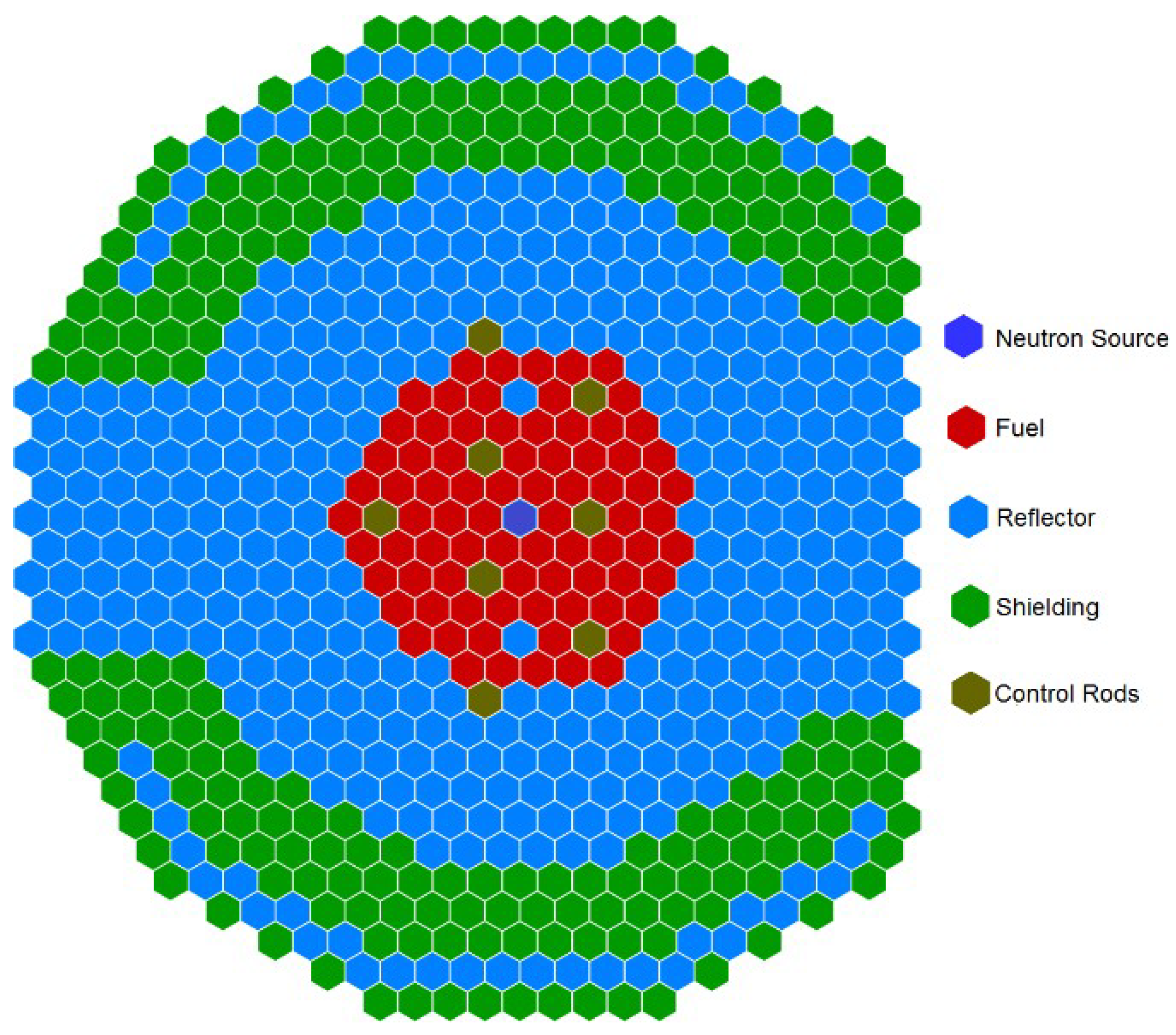
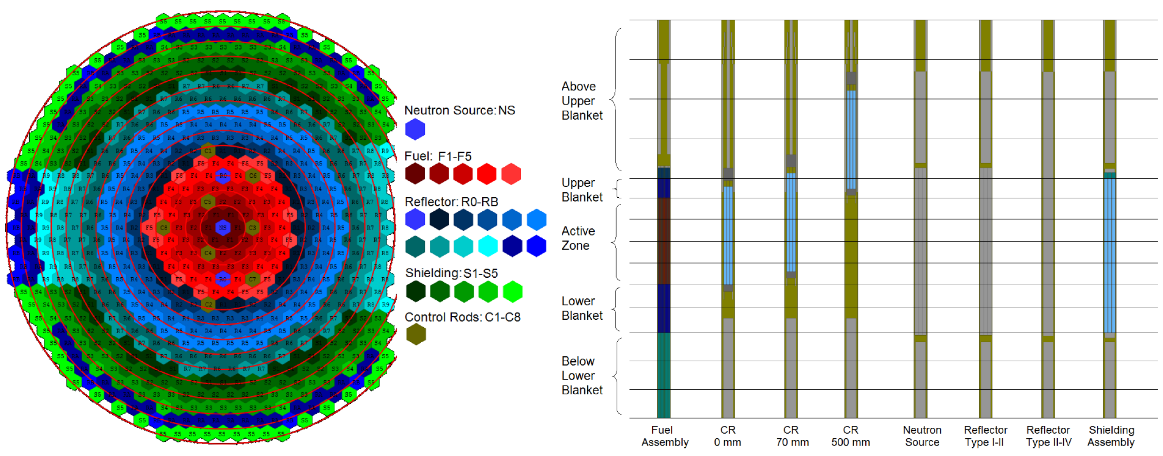
2. Description of China Experimental Fast Reactor

The China Experimental Fast Reactor (CEFR) is a 65 MWth pool-type sodium-cooled fast reactor constructed and operated by the China Institute of Atomic Energy (CIAE). It is the first fast reactor in China, which reached criticality for the first time in 2010. Figure 1 shows a cross-section of the reactor core, including the color identifiers of the in-core materials.
When fully loaded, a total of 79 fuel subassemblies (SAs) are present in the core, but it can reach criticality with only 72 and one control rod inserted at a certain height. The fuel SAs positions are originally occupied by Mock-Up fuel SAs, which are specially made SAs with similar geometry as regular fuel SAs but with no fuel present, and which are replaced by fuel SAs in stages. Other CEFR core components include 8 control rods SAs (3 safety rods, 3 shim rods, and 2 regulatory rods), 338 stainless steel SAs, 230 shielding SAs, and 1 neutron source SA [8].

3. Description of the Codes and Models

3.1. AZNHEX Code Background

The original AZNHEX code solves the neutron diffusion equation with elements of hexagonal-Z geometry. To do this, the code takes a hexagonal element and uses the Gordon-Hall transformation [11,12] to turn it into 4 squares in which the Raviart-Thomas-Nédélec order 0 (RTN-0) nodal method [13,14] can be applied for the spatial dependency of the equation. The interested reader can find a detailed description of the implementation in [2,15,16,17]. For the energy and time dependency, the code uses a multi-group approach and the θ method, respectively.
A previous effort on the code Verification and Validation process was done by means of the Benchmark for Neutronic Analysis of Sodium-cooled Fast Reactor Cores with Various Fuel Types and Core Sizes [18] organized by the Nuclear Energy Agency (NEA/OECD). The results showed good concordance with other participants in the Benchmark and were published in [2].
This previous effort showed that the results obtained by the diffusion code are good enough in a large-size core, nevertheless when it was used in a smaller core the deviation from the reference values was much higher. This can be since the diffusion model does not properly represent what happens in areas with high neutron leakage, which are much more present in a small core compared with a larger one. This proved the need for an improved solver for a wider range of accurate problem solving and, thus, justify the implementation of improved numerical models in the AZNHEX code.

S P L Implementation in AZNHEX

Proposed by Gelbard in the decade of 1960s [19,20,21], the S P L approximation is derived from the Spherical Harmonics Theory (the P L approximation) applied in the one-dimensional transport equation. This way, the original proposal consists of the simple replacement of the spatial partial derivatives in the one-dimensional form of the P L approximation by multivariable operators [19,22]. The resulting system of equations is made-up of a total of L   +   1 expressions per energy group, which is considerably easier to solve (even in time-dependent cases) than the ( L + 1 ) 2 system (per energy group) [23] of the three-dimensional, full spherical harmonics method.
The so-called canonical form of the S P L approximation, which is derived from the previously mentioned L   +   1 system, has been implemented in the AZNHEX code, re-shaping it to take the form of the neutron diffusion equation. The process that generates this diffusion-like equation also involves the calculation of “modified” cross-sections (XS) and diffusion coefficients, and the amount of these new values will depend on the order L selected by the user. Starting from the canonical form of the S P L approximation (Equation (1)):
μ n 2 Σ t g 2 Φ n g ( r ) + Σ t g Φ n g ( r )   =   g = 1 G Σ s 0 g g ϕ 0 g ( r ) + S 0 g ( r ) where n   =   1 , , L + 1 2 ,
and with the scalar neutron flux defined as follows (Equation (2)):
ϕ 0 g ( r )   =   n = 1 ( L + 1 ) / 2 ω n Φ n g ( r ) ,
where the value of Φ depends on the S P L index. If the sum is truncated after the first term when L   =   1 , Φ results equal to the scalar neutron flux ϕ 0 g (diffusion).
By replacing Equation (2) in the general form of S P L aproximation (Equation (1)) and expanding the neutron source term (without considering external sources), Equation (3) is obtained:
μ n 2 Σ t g 2 Φ n g ( r ) + Σ t g Φ n g ( r )   =   g = 1 G Σ s 0 g g m = 1 ( L + 1 ) / 2 ω m Φ m g ( r ) + 1 k χ g g = 1 G ν g Σ f g m = 1 ( L + 1 ) / 2 ω m Φ m g ( r ) ;
it is possible to manipulate Equation (3) to resemble a neutron diffusion-like equation for heterogeneous (Equation (4)) and homogeneous (Equation (5)) media since the goal of this is to be able to keep using the diffusion solver with only minimal modifications. Thus:
· D i ( r ) Φ i ( r ) + Σ R i ( r ) Φ i ( r )   =   j i ( ( L + 1 ) G ) / 2 Σ s i j ( r ) Φ j ( r ) + χ i j = 1 ( ( L + 1 ) G ) / 2 ν Σ f j ( r ) Φ j ( r )
and
D i 2 Φ i ( r ) + Σ R i Φ i ( r )   =   j i ( ( L + 1 ) G ) / 2 Σ s i j Φ j ( r ) + χ i j = 1 ( ( L + 1 ) G ) / 2 ν Σ f j Φ j ( r )
where: i   =   1 , , ( L + 1 ) G 2 ,
D i ( n , g )   =   μ n 2 Σ t g   =   3 μ n 2 D g , Σ R i ( n , g )   =   Σ t g ω n Σ s 0 g g , ν Σ f i ( n , g )   =   ω n ν g Σ f g , χ i ( n , g )   =   χ g , Σ s j ( m , g ) i ( n , g )   =   ω n Σ s 0 g g ,
with: d n , m = 1 , , L + 1 2 ; where g , g = 1 , , G ;
the terms μ n and ω n , which were introduced in Equations (1) and (2) and used to calculate the values of Equation (6), are constants that are calculated by solving the equation systems which come from the original L   +   1 system and that led to the canonical form of the S P L approximation. In the particular case of the implementation in AZNHEX, only S P 1 , S P 3 , S P 5 , and S P 7 were used, and their proper μ n and ω n values are given in Table 1.
As we mentioned before, the application of the S P L method in AZNHEX is aimed to odd values of L up to 7 (i.e., S P 1 , S P 3 , S P 5 , and S P 7 ). This way, considering that the number of XS and diffusion coefficient values will increase by two times for the S P 3 approximation, three times for the S P 5 approximation, and four times for the S P 7 approximation, the resulting system of diffusion-like equations for each odd order of L will increase the same way. To solve one of these systems, the AZNHEX code will implement an artificial energy mesh structure in which matrix size will vary according to the number of XS and diffusion coefficient new values (see [7] for full details on this implementation).
This method allows solving any three-dimensional energy-dependent problem without the need of using relatively high computational power and just by adding some minor modifications to the input file to be solved. Even if the user wants to implement the S P 7 approximation in the resolution of a given problem, it is expected that the required number of computational resources will be significantly less in comparison with a transport code. As a matter of example, if we consider a simple comparison of the number of unknowns to be found in a transport methodology, for instance in a Discrete Ordinates ( S N ) solver, with G energy groups and N C unknowns per discrete ordinate, if N is the order of discrete ordinate, the total number of unknowns ( T N U ) to be solved would be: T N U   =   N C × ( N + 2 ) × N × G . In the case of S P L approximation, T N U   =   N C × G × ( L + 1 ) / 2 , being L, the order of S P L approximation. In this case, assuming that the S N and S P L approximations are equivalent when N   =   L   +   1 , for an approximation S 8 in discrete ordinates T N U   =   80 × N C × G meanwhile, for S P 7 , T N U   =   4 × N C × G , i.e., 20 times less unknowns like in S 8 transport approach (8 times in the case of S 4 vs. S P 3 , and 16 times for the case of S 6 vs. S P 5 ). Of course, this analysis is done just in the number of unknowns of the problem independent from solvers and parallel algorithms that could be implemented in both methodologies. However, just having 20 times more unknowns as is the case for the transport S 8 implies that there is surely a big difference in computational time from what AZNHEX ( S P L ) would require.
Since the S P L approximation has its basis on a transport scheme, the results that are obtained through the implementation of this method are in general more accurate than the ones that are generated by using the conventional diffusion scheme. Nevertheless, it is important to mention that the design of this S P L solver has been made neglecting the higher-order transport effects of the expansion of the neutron scattering kernel. Additionally, the required boundary and interface conditions, which are specific for every odd order of the S P L approximation presented here, have not been included in the formulation of the S P L solver.

3.2. CEFR Core Modelling

3.2.1. Model for Serpent

Since AZNHEX is not able to generate its own XS, it is necessary to generate them by using another code. To perform this task, the Serpent code version 2.1.30 [24] was used due to its capability to generate macroscopic XS that can be employed to feed deterministic codes, which gives the opportunity to verify and validate the AZNHEX code by simulating more realistic scenarios and demonstrate its calculation capabilities. Additionally, the Serpent code is widely used in reactor calculations due to its high precision in 3D simulations and great capabilities and advantages over other Monte Carlo codes, which allow obtaining accurate reference solutions.
The 3D model of the CEFR reactor core was built considering the material specifications contained in the benchmark technical documentation such as the type of geometry of the core elements, their dimensions, the isotopic composition of the materials, etc. Since the experiments are carried out at different temperatures, thermal expansion effects have an impact on the materials, and they should be considered in the simulations. To simplify these calculations, we assumed that all the materials of the reactor core have the same linear expansion coefficient of 1.8 × 10 5 / C, which is the value for the stainless steel established in the benchmark specifications [8] and it is present in all the SAs. It also corresponds to the highest coefficient of the materials present in the core. To keep the same masses, the densities of all the materials were smeared except for the sodium coolant, whose density was always obtained using Equation (7) in agreement with technical specifications given in [8]. It is defined as:
ρ   =   950.0483 0.2298 T 14.604 × 10 6 T 2 + 5.6377 × 10 9 T 3 ,
where T is the temperature expressed in °C and ρ is the density in kg/m 3 .

3.2.2. Cross-Section (XS) Generation

To simplify the XS generation, the subassemblies (either fuel, control, reflector, or shielding) are grouped into rings of SAs of the same type. This methodology reduces considerably the amount of data that is handled. Additionally, all the subassemblies are divided into 14 axial zones; hence, for every ring of SAs, 14 sets of XS are generated. These XS are then extracted from Serpent through a Python script and are then used in AZNHEX. The core discretization can be seen in Figure 2.
For the XS energy multigroup structure, we used six energy groups when generating the XS sets, in agreement with the optimization of multi-group energy structures study presented in [25]. This number of energy groups is appropriate to reduce the computational time in nodal calculations with AZNHEX. The energy bins structure is shown in Table 2.
As an example, the group constants generated with Serpent in the axial zone 7 (from bottom to top as it can be seen in Figure 2 above) for the Fuel subassemblies grouped in Ring 1 (closest to the center of the core), are shown in Table 3.

4. Results

4.1. Verification and Validation Exercise

Since the fuel loading and criticality experiment is the one (among all Start-up experiments) that has direct reactivity values (and that can also be directly calculated with nodal solvers), we chose it for the verification and validation process of AZNHEX and to perform a sensitivity mesh refinement study. In this section, the fuel loading criticality exercise of the benchmark is described in detail, and the results obtained, first with Serpent and then with S P L implementation in AZNHEX and their comparison with the experimental data are presented.

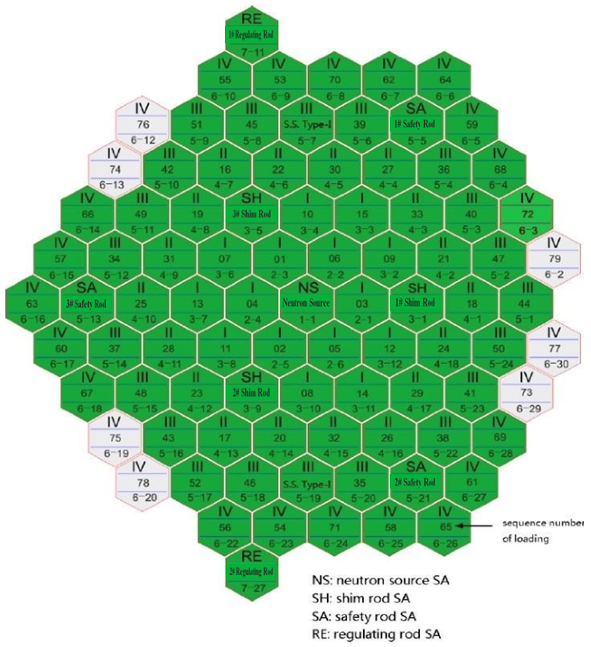
Description of Fuel Loading and Criticality Experiment

Before the start-up of the reactor, the core is preliminarily loaded with mock-up fuel SAs in the active fuel positions. The reactor moves to first criticality by replacing, step by step, the mock-up SAs with fuel SAs. In the sub-critical extrapolation process, the number of fuel SAs to be loaded is determined by extrapolation of reciprocal of count rate and following safety requirements; the process is described in [26] and shown in Figure 3.
When the core approaches to criticality, a super-critical extrapolation (that uses the control rods to reach criticality by the period method) is then used. In this extrapolation process, 72 fuel SAs were loaded. Control rods, with exception of one regulating rod that is fully inserted, are totally withdrawn to the out-of-core position. The regulating control rod is then withdrawn step by step to three different positions to reach super-criticality. At each position, a positive period is obtained. Based on that, the critical position of the control rod is predicted by extrapolation (based on the calculated control rod worth curve). Finally, the control rod is put to the predicted critical position, and the reactor’s clean-core criticality state is reached. For the CEFR, the final clean-core criticality state was reached with 72 fuel SAs and the regulating control rod at the position of 70 mm with a measured sodium temperature of 245 C. Three start-up detectors located near the active core (temporarily installed) were used to get the count rate throughout the criticality approaching process [26].

4.2. Verification and Validation of Serpent Model

Since calculations with codes directly provide the value of k e f f , we used the following equation to report the reactivity in each case:
ρ   =   ( k e f f 1.0 ) / k e f f ;
The reference calculation was the critical case. A study on the selection of the evaluated data library was done to ensure that the numerical results calculated with both Serpent and AZNHEX, would have minimum differences in comparison with those obtained experimentally. Thus, eight different libraries were tested with the same Serpent model (for the critical case). The evaluated data files were: BROND-3.1 [27], CENDL-3.1 [28], ENDF/B-VII.1 [29], ENDF/B-VIII.0 [30], JEFF-3.1 [31], JEFF-3.1.2 [32], JEFF-3.2 [33] and JENDL-4.0 [34].
As mentioned in Section 4.1, the core was modeled with 72 fuel SAs inserted and all control rods (CRs) out (position 500 mm) except for the Regulating Rod 2 (RE2) which is inserted in position 70 mm. This state was selected because the core is expected to reach criticality under those conditions, as experiments showed [8].
The exercise showed that the ENDF/B-VIII.0 library is the best suited for this case, resulting in a reactivity of only 4 pcm above the expected reactivity value ( ρ e x p   =   0.0 for the critical case), as shown in Figure 4.
For this reason, we selected the ENDF/B-VIII.0 library for all the numerical calculations done in this work.
The results of the Serpent model for the expected calculations in terms of reactivity, with an estimated value of 0.0 in the final critical position, are presented in Table 4.

4.3. Verification and Validation of S P L Implementation in AZNHEX

Table 5 shows the reactivity values obtained from the AZNHEX k e f f results employing all the S P L approximations and the deviation of these results with respect to the experimental data for the supercritical and critical steps.
The original version of AZNHEX only included the diffusion approximation ( S P 1 ) and, as expected, the results obtained with the S P 1 approximation have the highest discrepancies compared with the experimental values and with other S P L approximations since the S P 1 method corresponds to diffusion and is not able to properly represent the real conditions in this kind of small and high leaking fast reactors. It is clear that as the index of the S P L approximation increases, the results are more accurate when compared with the reference results, with differences below 200 pcm in the S P 5 and S P 7 cases.
In Figure 5, the same results of Table 5 are presented but in k e f f values, where it is possible to appreciate the difference in employing different S P L approximations.
Regarding the computational times, in Table 6, a comparison among the different times of S P L approximations is done. It can be seen that, there is a significative difference between S P 1 and S P 3 (and, of course, with the other S P 5 and S P 7 approximations). The reason is due to the fact that, in the original version of AZNHEX (pure diffusion implementation), the scattering matrix is numerically adjusted in order to avoid up-scattering terms, for this reason, the inner iteration process finalized in significant less steps. However, in the methodology used in this S P L implementation, and described with detail in [7], the introduction of higher orders of S P L implies the creation of pseudo energy-groups, i.e., the original matrix (diffusion) is expanded with the new S P L coefficients. The order of the matrix is multiplied by 2, 3, and 4, respectively for S P 3 , S P 5 , and S P 7 including “up-scattering” terms between pseudo groups. The consequence of this artificial up-scattering effect, results in an increase of the inner iterations, and thus of the computational times almost for 10 times between S P 1 and S P 3 . It could be significant amount of time, however, such implementation allows us to move from more than 2000 pcms of difference to 350 pcms. In the final line of Table 6, it is possible to see the time factor between the S P 5 and S P 7 , comparing with S P 3 , in this case, the result is very consistent with the size of the matrix to be solved in each case.
In Figure 6, the normalized radial power distribution obtained with Serpent and AZNHEX S P 1 to S P 7 , with a 2   ×   2 mesh refinement, is shown. The mesh refinement applied in AZNHEX is described in the following subsection. The values were normalized to 1, this is, the average power value is equal to 1. The figure presents also, the path line to track the power. As it can be seen, the maximum value is located in the first assembly, which is near to the center of the core, for all the calculations. The AZNHEX results present higher discrepancies in the border of the core (point 5) which can be related to the high leakage effect in this interphase.

Mesh Sensitivity Analysis with AZNHEX S P L

An extra analysis was performed for this exercise in which different mesh refinements were implemented to approximate even better the AZNHEX results to the experimental data. These refinements were done radially and axially along the reactor core. For a deeper analysis, besides the combination of radial and axial refinements, both refinements were also done separately. Figure 7 and Figure 8 show the way these radial and axial refinements are done in AZNHEX.
The Table 7 shows the reactivity values obtained from the AZNHEX k e f f results employing the S P L approximations with radial refinement and the deviation of these results from the experimental data.
It can be seen in Table 7 that larger differences are obtained with the radial refinements in comparison with the no refinement cases ( 1 × 1 ) for all S P L approximations in the four cases of approach to criticality process, getting the best results with the S P 7 _ 1 × 1 refinement. Additionally, Table 8 shows the reactivity values obtained from the AZNHEX k e f f results employing the S P L approximations with only axial refinement and the deviation of these results concerning the experimental data. It is possible to observe that, with exception of S P 3 approximation, the axial refinement has significant reactivity differences. The main reason, could be related with the increase in the dimensions ratio between axial and radial nodes. The aspect ratio is defined as the ratio of the longest dimension to the shortest dimension of a quadrilateral element. In many cases, as the aspect ratio increases, the inaccuracy of the solution increases, and in general, an element yields best results if its shape is compact and regular, a more detailed description of this phenomenon is presented in [35].
In order to decrease the aspect ratio and to make shape compact and more regular, a combination of radial and axial refinements was used. In Table 9 the reactivity values obtained from the AZNHEX k e f f results employing the S P L approximations by using both radial and axial refinements and the deviation of these results from the experimental data are shown.
It is possible to see that a better consistency in the results is obtained when combined refinements (axial and radial) are used, mainly in the highest order S P L approximations ( S P 5 and S P 7 ) obtaining the best results with the S P 7 _ 4 × 4 refinement approximation, having differences below 11 pcm.
The computational cost of such refinement is presented in Table 10. It is possible to see that, in general, moving from no refinement ( 1 × 1 ) to full refinement ( 4 × 4 ) increases the computational time with a factor of approximately 60 whereas for an intermediate refinement ( 2 × 2 ) the computational time just increases 7.5 times. From Table 9, for S P 5 and S P 7 , 2   ×   2 results are very acceptable and the computational time is also suitable, thus, a 2   ×   2 refinement could be seen as an optimal election.

5. Discussion

Constant improvement is part of the software development. Even though the original version of the AZNHEX code was successfully tested in a previous set of exercises, it failed when used in a smaller core; therefore, an improvement on the mathematical solver was needed. In this work, a recently developed S P L solver (based on the Spherical Harmonics Theory), along with its validation process, were presented. As part of the objectives of the AZTLAN Platform, the designing and incorporation into AZNHEX of this S P L solver are aimed to increase the numerical precision of the code itself, making AZNHEX a reliable computational tool for designing and analyzing nuclear reactors made up of subassemblies with hexagonal-z geometry such as the Russian Lead-Cooled Fast Reactor, BREST [36] under development, the Korean Sodium-Cooled Fast Reactor, KALIMER [37] and the Advanced Lead Fast Reactor European Demonstrator, ALFRED [38]. This is especially relevant since the newest generations of nuclear reactors are characterized by this hexagonal-z geometry of its subassemblies.
The structure of the S P L solver incorporated into AZNHEX allows its relatively easy implementation in other diffusion codes of the AZTLAN Platform, since there is only the need of modifying the values of the XS and the diffusion coefficients into an artificial array of energy groups.
On the other hand, the methodology employed to generate the XS data with Serpent was very useful to simplify the amount of data to handle for the AZNHEX models in conjunction with the use of 6 neutron energy groups. This resulted in a considerable reduction of the computing time in both codes and in to getting very accurate results with AZNHEX, as can be seen in this paper.
About the results themselves, a great improvement was seen when using the new S P L solver in AZNHEX, getting very similar values to those obtained with Serpent and with the experimental ones. Referring to the data shown in Table 5, it can be seen that the major improvement in the precision of the results occurs between the S P 1 and the S P 3 approximations. Although the S P 5 and the S P 7 schemes offer results that are closer to the reference data, the implied computational cost of solving a given problem through such approximations is, in most cases, unnecessarily expensive for the desired precision. Furthermore, the data presented in Table 7, Table 8 and Table 9 allow considering in detail the impact of the radial and axial refinements. Although a reduction of the deviation with increased S P L refinements was expected, many values within these results present a different behavior. For example, in Table 7, it can be seen that, for the diffusion approximation ( S P 1 ), the deviation is smaller as the radial refinement increases. Nevertheless, for the S P 3 , S P 5 , and S P 7 schemes, the absolute deviation shows a trend to increase along with the radial refinement. Besides, the absolute deviations for the S P 7 approximation, considering superior radial refinements, are bigger than the equivalent values for the S P 5 approximation. Additionally, for the reactivity data shown in Table 8, the impact of the axial refinement behaves somewhat differently. While the absolute deviation increases alongside the axial refinement for every order of the S P L approximation but the S P 3 approximation, such deviations are smaller as the odd order of L increases.
In order to tackle such inconsistencies (maybe related to the big differences on radial and axial sizes), a combined radial and axial refinement was used. In this case, a better consistency in the results is obtained mainly in the highest order S P L approximations ( S P 5 and S P 7 ) where the best results were obtained, as expected, with the S P 7 _ 4 × 4 refinement approximation.
However, it is important to clarify that some of the previously mentioned unexpected variations in the reactivity deviations could be attributed to the absence of the aforementioned superior transport effects of the scattering kernel and, to a lesser extent, to the lack of the required interface and boundary conditions. Since one of the main advantages of the S P L approximation is its higher precision in the description of the scalar neutron flux in highly heterogeneous media, the absence of the anisotropic behavior of the neutron scattering has a significant effect in small cells where the non-consistent change in the spatial dimensions could affect the flux gradient. We planned further investigations in this direction [39].

6. Conclusions

Despite the unexpected changes in the reactivity deviations, it can be concluded that the implementation of the S P L module in the current version of AZNHEX fulfilled the objective to improve the estimation of the results for a small fast reactor such as the CEFR. More accurate estimations were obtained using S P 5 and S P 7 approximations in most of the exercises, where the differences concerning the experimental values were around 100 pcm. This indicates that higher L values lead to relatively closer values to the reference data having also lower computational times in comparison with a stochastic code.
Further development of the S P L solver described in this work involves the restructuring of its mathematical background to appropriate include the higher order elements of the expansion of the scattering kernel with the required interface and boundary conditions, to describe with more precision the neutron scalar flux and every involved anisotropy term. It is expected that such a restructuring process allows to correct the variations of the reactivity deviations, despite the implemented order of the S P L approximation.
Additionally, the restructuring of the S P L solver includes the addition of a time-dependent module, which will allow analyzing phenomena such as the variations of the scalar neutron flux and the reactivity deviations as the rods within the core move from one position to another.
Finally, a Discrete Ordinates S N module is also being implemented in AZNHEX. Further work will be performed to compare these new solvers against stochastic and experimental data.

Author Contributions

Conceptualization, A.G.-T. and E.d.V.-G.; methodology, R.L.-S. and J.G.-A.; software, G.M.-P.; validation, G.M.-P., R.L.-S. and J.G.-A.; formal analysis, A.G.-T., E.d.V.-G.; investigation, G.M.-P.; resources, A.G.-T.; data curation, G.M.-P. and E.d.V.-G.; writing—original draft preparation, J.G.-A., R.L.-S., G.M.-P.; writing—review and editing, A.G.-T. and E.d.V.-G.; project administration, A.G.-T. and E.d.V.-G.; funding acquisition, A.G.-T. All authors have read and agreed to the published version of the manuscript.

Funding

This research was funded by the: Programa Presupuestario F003, Programas Nacionales Estratégicos de Ciencia, Tecnología y Vinculación con los Sectores Social, Público y Privado, 212602 (AZTLAN Platform).

Data Availability Statement

Not applicable.

Conflicts of Interest

The authors declare no conflict of interest. The funders had no role in the design of the study; in the collection, analyses, or interpretation of data; in the writing of the manuscript; or in the decision to publish the results.

Abbreviations

The following abbreviations are used in this manuscript:
AZNHEXAZtlan Nodal HEXagonal
AZKINDAZtlan KInetics in Neutron Diffusion
AZTHECAAZtlan THErmohydraulics Core Analysis
AZTRANAZtlan TRANsport
AZTUSIAAZtlan Tool for Uncertainty and SensItivity Analysis
BRONDLibrary of Recommended Evaluated Neutron Data (in Russian abbreviations)
CEFRChina Experimental Fast Reactor
CENDLChinese Evaluated Nuclear Data Library
CIAEChina Institute of Atomic Energy
CONACYTNational Council for Science and Technology (in Spanish abbreviations)
ENDFEvaluated Nuclear Data File
IAEAInternational Atomic Energy Agency
ININNational Institute of Nuclear Research (in Spanish abbreviations)
IPNNational Polytechnic Institute (in Spanish abbreviations)
JEFFJoint Evaluated Fission and Fusion File
JENDLJapanese Evaluated Nuclear Data Library
NEANuclear Energy Agency
OECDOrganisation for Economic Co-operation and Development
SENERSecretariat of Energy (in Spanish abbreviations)

Nomenclature

Symbols
D g Diffusion coefficient for energy group g, m
D i Diffusion coefficient for artificial energy-group i, m
gEnergy group g
g Energy group g
GTotal number of energy groups considered in a given problem
iInteger number that describes the array of the diffusion coefficients and
cross-sections depending on the energy group g and the order L implemented
jInteger number that describes the array of the diffusion coefficients and
cross-sections depending on the energy group g and the order L implemented
kMultiplication factor
k e f f Effective multiplication factor
LImplemented order of the S P L approximation
mInteger number that identifies the implemented ( L + 1 ) / 2 order of the S P L
approximation
NOrder of discrete ordinate
N C Number of unknowns per discrete ordinate
nInteger number that identifies the implemented ( L + 1 ) / 2 order of the S P L
approximation
pcmpercent mili-rho
r A vector that indicates the spatial position of a neutron in a three-dimensional space
S l g l-th angular moment of the neutron source term for energy group g , 1/m 3 · s
T N U Total number of unknowns
μ m , μ n S P L -order dependent constant
ν g Average number of neutrons released by fissions which are induced by neutrons
with energies in the energy group g
ν g Average number of neutrons released by fissions which are induced by
neutrons with energies in the energy group g
ν Σ f i Macroscopic fission cross-section multiplied by the average number of
neutrons produced per fission, for artificial energy-group i, 1/m
ν Σ f j Macroscopic fission cross-section multiplied by the average number of
neutrons produced per fission, for artificial energy-group j, 1/m
ρ Reactivity
Σ f g Macroscopic fission cross-section for energy group g, 1/m
Σ f g Macroscopic fission cross-section for energy group g , 1/m
Σ R i Macroscopic removal cross-section for artificial energy-group i, 1/m
Σ s 0 g g 0-th angular moment of the macroscopic scattering cross-section from energy
group g to energy group g, 1/m
Σ s 0 g g 0-th angular moment of the macroscopic scattering cross-section from energy
group g to energy group g, 1/m
Σ s j i Macroscopic scattering cross-section from artificial energy-group j to artificial
energy-group i, 1/m
Σ t g Macroscopic total cross-section for energy group g, 1/m
ϕ 0 g Scalar neutron flux for energy group g, 1/m 2 · J·s
ϕ 0 g Scalar neutron flux for energy group g , 1/m 2 · J·s
Φ i Array of neutron flux moments for artificial energy-group i, 1/m 2 · s
Φ j Array of neutron flux moments for artificial energy-group j, 1/m 2 · s
Φ m g m-th array of neutron flux moments for energy group g , 1/m 2 · s
Φ n g n-th array of neutron flux moments for energy group g, 1/m 2 · s
χ g Probability that a neutron is born in the energy group g
χ i Neutron fission spectrum for artificial energy-group i
ω m , ω n S P L -order dependent constant
Gradient
· Divergence
2 Laplace operator

References

  1. Gómez-Torres, A.M.; Puente-Espel, F.; del-Valle-Gallegos, E.; François-Lacouture, J.L.; Martin-del-Campo, C.; Espinosa-Paredes, G. AZTLAN: Mexican Platform for Analysis and Design of Nuclear Reactors. In Proceedings of the International Congress on Advances in Nuclear Power Plants (ICAPP), Nice, France, 3–6 May 2015. [Google Scholar]
  2. Duran-González, J.; del-Valle-Gallegos, E.; Reyes-Fuentes, M.; Gómez-Torres, A.M.; Xolocostli-Munguía, V. Development, verification, and validation of the parallel transport code AZTRAN. Prog. Nucl. Energy 2021, 137, 103792. [Google Scholar] [CrossRef]
  3. Rodríguez-Hernández, A.; Gómez-Torres, A.M.; del-Valle-Gallegos, E. Hpc implementation in the time-dependent neutron diffusion code AZKIND. Ann. Nucl. Energy 2017, 99, 174–182. [Google Scholar] [CrossRef]
  4. Del-Valle-Gallegos, E.; Lopez-Solis, R.; Arriaga-Ramirez, L.; Gomez-Torres, A.; Puente-Espel, F. Verification of the multi-group diffusion code AZNHEX using the OECD/NEA UAM Sodium Fast Reactor Benchmark. Ann. Nucl. Energy 2018, 114, 592–602. [Google Scholar] [CrossRef]
  5. Reyes-Fuentes, M.; del-Valle-Gallegos, E.; Duran-González, J.; Ortíz-Villafuerte, J.; Castillo-Durán, R.; Gómez-Torres, A.M.; Queral, C. AZTUSIA: A new application software for Uncertainty and Sensitivity analysis for nuclear reactors. Reliab. Eng. Syst. 2021, 209, 107441. [Google Scholar] [CrossRef]
  6. Campos-Muñoz, A. Development of a 3-D Neutron Transport Solver for the AZNHEX Code. Master’s Thesis, National Polytechnic Institute, Superior School of Physics and Mathematics, Mexico City, Mexico, 2021. [Google Scholar]
  7. Muñoz-Peña, G.; del-Valle-Gallegos, E.; Gómez-Torres, A.M. Canonical implementation of Simplified Spherical Harmonics (SPL) in the neutron diffusion code AZNHEX. ASME J. Nucl. Eng. Radiat. Sci. 2021, 7, 031502. [Google Scholar] [CrossRef]
  8. Huo, X. Technical Specifications for Neutronics Benchmark of CEFR Start-Up Tests, Version 7.0. KY-IAEA-CEFRCRP-001; China Institute of Atomic Energy: Beijing, China, 2019. [Google Scholar]
  9. Wan, C.; Qiao, L.; Zheng, Y.; Cao, L.; Wu, H. Validation of SARAX for the China Fast Reactor with the extrapolated experimental data. Ann. Nucl. Energy 2019, 127, 188–195. [Google Scholar] [CrossRef]
  10. Du, X.; Choe, J.; Quoc-Tran, T.; Lee, D. Neutronic simulation of China Experimental Fast Reactor start-up tests. Part I: SARAX code deterministic calculation. Ann. Nucl. Energy 2020, 136, 107046. [Google Scholar] [CrossRef]
  11. Gordon, W.J.; Hall, C.A. Transfinite element methods: Blending–function interpolation over arbitrary curved element domains. Numer. Math. 1973, 21, 109–129. [Google Scholar] [CrossRef]
  12. Gordon, W.J.; Hall, C.A. Construction of curvilinear co-ordinate systems and applications to mesh generation. Int. J. Numer. Methods Eng. 1973, 7, 461–477. [Google Scholar] [CrossRef]
  13. Brezzi, F.; Douglas, J.; Marini, L.D. Two Families of Mixed Finite Elements for Second Order Elliptic Problems. Numer. Math. 1985, 47, 217–235. [Google Scholar] [CrossRef]
  14. Raviart, P.A.; Thomas, J.M. A mixed finite element method for 2-nd order elliptic problems. In Mathematical Aspects of Finite Element Methods; Galligani, I., Magenes, E., Eds.; Springer: Heidelberg, Germany, 2006; pp. 292–315. [Google Scholar]
  15. Del-Valle-Gallegos, E. Nodal Methods in Particle Transport and Diffusion. Ph.D. Thesis, National Polytechnic Institute, Superior School of Physics and Mathematics, Mexico City, Mexico, 1998. [Google Scholar]
  16. Esquivel-Estrada, J. Nodal Methods Applied to the Time-Dependent Neutron Diffusion Equation in Hexagonal-Z Geometry. Master’s Thesis, National Polytechnic Institute, Superior School of Physics and Mathematics, Mexico City, Mexico, 2015. [Google Scholar]
  17. Gomez Torres, A.; Lopez Solis, R.C.; Puente Espel, F.; Valle Gallegos, E.D.; Arriaga Ramirez, L.; Fridman, E.; Kliem, S. Verification of the neutron diffusion code AZNHEX by means of the Serpent-DYN3D and Serpent-PARCS solution of the OECD/NEA SFR Benchmark. In Proceedings of the International Congress on Advances in Nuclear Power Plants (ICAPP), Yekaterinburg, Russia, 26–29 June 2017. [Google Scholar]
  18. Blanchet, D.; Buiron, L.; Stauff, N.; Kim, T.K.; Taiwo, T. AEN WPRS Sodium Fast Reactor Core Definitions (Version 1.5 Revision 10); OECD Nuclear Energy Agency: Paris, France, 2017. [Google Scholar]
  19. Gelbard, E.M. Application of Spherical Harmonics Method to Reactor Problems; Tech. Rep. WAPD-BT-20; Bettis Atomic Power Laboratory: Pittsburgh, PA, USA, 1960. [Google Scholar]
  20. Gelbard, E.M. Simplified Spherical Harmonics Equations and Their Use in Shielding Problems; Tech. Rep. WAPD-T-1182; Bettis Atomic Power Laboratory: Pittsburgh, PA, USA, February 1961. [Google Scholar]
  21. Gelbard, E.M. Applications of the Simplified Spherical Harmonics Equations in Spherical Geometry; Tech. Rep. WAPD-TM-294; Bettis Atomic Power Laboratory: Pittsburgh, PA, USA, 1962. [Google Scholar]
  22. Gelbard, E.M. Spherical harmonics methods: PL and double-PL approximations. In Computing Methods in Reactor Physics; Greenspan, H., Kelber, C.N., Okrent, D., Eds.; Gordon and Breach Science Publishers: New York, NY, USA, 1968; Chapter 4. [Google Scholar]
  23. Dürigen, S. Neutron Transport in Hexagonal Reactor Cores Modeled by Trigonal-Geometry Diffusion and Simplified P3 Nodal Methods. Ph.D. Thesis, Karlsruhe Institute of Technology, Department of Mechanical Engineering, Karlsruhe, Germany, 2013. [Google Scholar]
  24. Leppänen, J.; Pusa, M.; Viitanen, T.; Valtavirta, V.; Kaltiaisenaho, T. The Serpent Monte Carlo code: Status, development and applications in 2013. Ann. Nucl. Energy 2015, 82, 142–150. [Google Scholar] [CrossRef]
  25. Di-Nora, V.A.; Fridman, E.; Nikitin, E.; Bilodid, Y.; Mikityuk, K. Optimization of multi-group energy structures for diffusion analyses of sodium-cooled fast reactors assisted by simulated annealing—Part I: Methodology demonstration. Ann. Nucl. Energy 2021, 155, 108183. [Google Scholar] [CrossRef]
  26. Gómez-Torres, A.M.; Lopez-Solis, R.C.; Galicia-Aragon, J.; Huo, X.; Kriventsev, V.; Batra, C.; Kim, T.K.; Jarret, M.; Fridman, E.; Zheng, Y.; et al. Verification and validation of neutronic codes using the start-up fuel load and criticality tests performed in the China Experimental Fast Reactor. In Proceedings of the International Conference on Fast Reactors and Related Fuel Cycles: Sustainable Clean Energy for the Future (FR22), Vienna, Austria, 19–22 April 2022. [Google Scholar]
  27. Blokhin, A.I.; Gai, E.V.; Ignatyuk, A.V.; Koba, I.I.; Manokhin, V.N.; Pronyaev, V.G. New Version of Neutron Evaluated Data Library Brond-3.1. Probl. At. Sci. Technol. Ser. Nucl. React. Constants 2016, 2, 62–93. [Google Scholar]
  28. Zhigang, G.; Hongwei, Y.; Youxiang, Z.; Tingjin, L.; Jingshang, Z.; Ping, L.; Haicheng, W.; Zhixiang, Z.; Haihong, X. The updated version of Chinese Evaluated Nuclear Data Library (CENDL-3.1) and China nuclear data evaluation activities. In Proceedings of the IAEA Technical Meeting in collaboration with NEA on Specific Applications of Research Reactors: Provision of Nuclear Data, Vienna, Austria, 12–16 October 2009. [Google Scholar]
  29. Brown, D.A. Release of the ENDF/B-VII.1 Evaluated Nuclear Data File. In Proceedings of the 2012 ANS Winter Meeting, San Diego, CA, USA, 11–15 November 2012. [Google Scholar]
  30. Brown, D.A.; Chadwick, M.B.; Capote, R.; Kahler, A.C.; Trkov, A. ENDF/B-VIII.0: The 8th Major Release of the Nuclear Reaction Data Library with CIELO-project Cross Sections, New Standards and Thermal Scattering Data. Nucl. Data Sheets 2018, 148, 1–142. [Google Scholar] [CrossRef]
  31. Koning, A.; Forrest, R.; Kellett, M.; Mills, R.; Henriksson, H.; Rugama, Y. The JEFF-3.1 Nuclear Data Library-JEFF Report 21; NEA-OECD: Paris, France, 2006; ISBN 92-64-02314-3. [Google Scholar]
  32. Santamarina, A.; Bernard, D.; Blaise, P.; Coste, M.; Courcelle, A.; Huynh, T.D.; Jouanne, C.; Leconte, P.; Litaize, O.; Mengelle, S.; et al. The JEFF-3.1 Nuclear Data Library-JEFF Report 22; NEA-OECD: Paris, France, 2009; ISBN 978-92-64-99074-6. [Google Scholar]
  33. Glinatsis, G.; Carta, M.; Gugiu, D.; Ikonomopoulos, A.; Visan, I. An investigation of the JEFF 3.2 nuclear data library. Ann. Nucl. Energy 2022, 168, 108885. [Google Scholar] [CrossRef]
  34. Shibata, K.; Iwamoto, O.; Nakagawa, T.; Iwamoto, N.; Ichihara, A.; Kunieda, S.; Chiba, S.; Furutaka, K.; Otuka, N.; Ohsaw, T.; et al. JENDL-4.0: A New Library for Nuclear Science and Engineering. J. Nucl. Sci. Technol. 2011, 48, 1–30. [Google Scholar] [CrossRef]
  35. Logan, D.L. A First Course in the Finite Element Method, 4th ed.; Thomson: Toronto, ON, Canada, 2007; p. 351. [Google Scholar]
  36. Adamov, E.O.; Kaplienko, A.V.; Orlov, V.V. Brest Lead-Cooled Fast Reactor: From Concept to Technological Implementation. At. Energy 2021, 129, 179–187. [Google Scholar] [CrossRef]
  37. Kim, Y.; Lee, Y.B.; Lee, C.B.; Chang, J.; Choi, C. Design Concept of Advanced Sodium-Cooled Fast Reactor and Related R & D in Korea. Sci. Technol. Nucl. Install. 2013, 2013, 290362. [Google Scholar] [CrossRef] [Green Version]
  38. Frogheri, M.; Alemberti, A.; Mansani, L. The Lead Fast Reactor: Demonstrator (ALFRED) and ELFR Design. In Proceedings of the International Conference on Fast Reactors and Related Fuel Cycles: Safe Technologies and Sustainable Scenarios (FR13), Paris, France, 4–7 March 2013. [Google Scholar]
  39. Muñoz-Peña, G. Development, Verification, and Validation of an Improved Version of the AZNHEX Code of the AZTLAN Platform, Including Feedback. Ph.D. Thesis, National Polytechnic Institute, Superior School of Physics and Mathematics, Mexico City, Mexico, 2022. in preparation. [Google Scholar]
Figure 1. CEFR Core Layout.
Jne 04 00005 g001
Figure 2. Radial and Axial Division of the CEFR Core.
Jne 04 00005 g002
Figure 3. Loading configuration of the clean core.
Jne 04 00005 g003
Figure 4. Reactivities calculated on the XS library test.
Jne 04 00005 g004
Figure 5. k e f f values obtained with AZNHEX- S P L and their comparison with the experimental data.
Jne 04 00005 g005
Figure 6. Normalized radial power distribution.
Jne 04 00005 g006
Figure 7. Radial (a 1 × 1 , (b) 2 × 2 , (c) 3 × 3 , and (d) 4 × 4 refinements made in the AZNHEX code.
Jne 04 00005 g007
Figure 8. Axial (a × 1 , (b) × 2 , (c) × 3 , and (d) × 4 refinements made in the AZNHEX code.
Jne 04 00005 g008
Table 1. Values of constants μ n y ω n for given S P L aproximation order.
n = 1,⋯,(L+1)/2μnωn
L = 1
1 1 / 3 1
L = 3
10.3399810435848560.652145154862546
20.8611363115940530.347854845137454
L = 5
10.2386191860831970.467913934572691
20.6612093864662650.360761573048139
30.9324695142031520.171324492379170
L = 7
10.1834346424956500.362683783378360
20.5255324099163290.313706645877890
30.7966664774136270.222381034453374
40.9602898564975360.101228536290376
Table 2. Neutron energy groups employed.
GroupUpper Limit (MeV)
12.000000 × 10 1
21.353400 × 10 0
35.23400 × 10 1
46.73790 × 10 2
53.35460 × 10 3
67.48520 × 10 4
Table 3. Group constants generated with Serpent.
MaterialEnergy
Group
Group Constants
D g Σ r g ν Σ f g κ Σ f g χ g Σ s g g
Fuel SA’s
(Ring 1)
12.9684.290 × 10 2 2.205 × 10 2 2.031 × 10 2 5.794 × 10 1 1.220 × 10 1 2.474 × 10 2 8.885 × 10 3
3.425 × 10 4 2.323 × 10 6 4.666 × 10 7
22.1502.978 × 10 2 1.529 × 10 2 2.023 × 10 2 2.825 × 10 1 0.001.739 × 10 1 2.223 × 10 2
4.088 × 10 4 3.151 × 10 6 1.542 × 10 7
31.5271.407 × 10 2 1.747 × 10 2 2.022 × 10 2 1.303 × 10 1 0.000.002.352 × 10 1
4.892 × 10 3 1.206 × 10 6 6.873 × 10 8
41.0661.811 × 10 2 2.767 × 10 2 2.022 × 10 2 7.495 × 10 3 0.000.000.00
3.248 × 10 1 1.253 × 10 3 8.235 × 10 7
56.931 × 10 1 5.512 × 10 2 7.978 × 10 2 2.022 × 10 2 8.053 × 10 5 0.000.000.00
0.005.400 × 10 1 3.866 × 10 3
67.796 × 10 1 9.172 × 10 2 1.488 × 10 1 2.022 × 10 2 9.843 × 10 6 0.000.000.00
0.000.003.634 × 10 1
Table 4. Reactivity values and deviation in pcm from Serpent calculations and experimental data.
RE2 PositionExp. MeasurementSerpentAbsolute Dev.
ρ exp (pcm) ρ Serpent (pcm) ρ exp ρ Serpent
190 mm4048.0−8.0
170 mm3441.0−7.0
151 mm2528.0−3.0
70 mm04.0−4.0
Table 5. Reactivity values and deviation in pcm from AZNHEX calculations and experimental data.
RE2 PositionExp. MeasurementAZNHEX (pcm)
ρ exp ρ SP 1 Dev ρ SP 3 Dev ρ SP 5 Dev ρ SP 7 Dev
190 mm40−2031.342071.34356.52−316.52−143.08183.08−123.57163.57
170 mm34−2032.812066.81355.13−321.13−144.24178.24−124.73158.73
151 mm25−2038.182063.18349.97−324.97−149.21174.21−129.70154.70
70 mm0−2065.012065.01324.15−324.15−174.29174.29−154.75154.75
Table 6. Comparison of computational times for different S P L approximations.
SP 1 SP 3 SP 5 SP 7
Time [s]237.72260.44244.96546.5
Time factor vs. S P 1 19.517.827.5
Time factor vs. S P 3 11.82.9
Table 7. Reactivity values and deviation in pcm from AZNHEX calculations with radial refinement and experimental data.
RE2 Position 190 mmDev170 mmDev151 mmDev70 mmDev
Exp.
Measurement 40 (pcm)34 (pcm)25 (pcm)0 (pcm)
S P 1 _ 1 × 1 −2031.342071.34−2032.812066.81−2038.182063.18−2065.012065.01
S P 1 _ 2 × 1 −1649.181689.18−1650.811684.81−1656.311681.31−1683.731683.73
S P 1 _ 4 × 1 −1508.351548.35−1510.341544.34−1515.891540.89−1543.481543.48
S P 3 _ 1 × 1 356.72−316.72354.74−320.74349.77−324.77323.95−323.95
S P 3 _ 2 × 1 702.06−662.06700.42−666.42695.17−670.17668.81−668.81
AZNHEX S P 3 _ 4 × 1 827.93−787.93826.24−792.24821.08−796.08794.40−794.40
S P 5 _ 1 × 1 −143.20183.20−144.21178.21−149.22174.22−174.30174.30
S P 5 _ 2 × 1 202.30−162.30201.03−167.03195.93−170.93170.28−170.28
S P 5 _ 4 × 1 327.31−287.31326.01−292.01320.88−295.88295.01−295.01
S P 7 _ 1 × 1 −124.15164.15−125.16159.16−130.17155.17−155.24155.24
S P 7 _ 2 × 1 221.92−181.92220.65−186.65215.56−190.56189.99−189.99
S P 7 _ 4 × 1 346.73−306.73345.43−311.43340.30−315.30314.57−314.57
Table 8. Reactivity values and deviation in pcm from AZNHEX calculations with axial refinement and experimental data.
RE2 Position 190 mmDev170 mmDev151 mmDev70 mmDev
Exp.
Measurement 40 (pcm)34 (pcm)25 (pcm)0 (pcm)
S P 1 _ 1 × 1 −2031.342071.34−2032.812066.81−2038.182063.18−2065.012065.01
S P 1 _ 1 × 2 −2302.142342.14−2303.702337.70−2309.082334.08−2336.422336.42
S P 1 _ 1 × 4 −2374.522414.52−2376.132410.13−2381.542406.54−2408.992408.99
S P 3 _ 1 × 1 356.72−316.72354.74−320.74349.77−324.77323.95−323.95
S P 3 _ 1 × 2 99.90−59.9098.90−64.9092.91−67.9166.96−66.96
AZNHEX S P 3 _ 1 × 4 28.9911.0127.996.0122.003.00−4.004.00
S P 5 _ 1 × 1 −143.20183.20−144.21178.21−149.22174.22−174.30174.30
S P 5 _ 1 × 2 −398.58438.58−399.59433.59−404.63429.63−430.85430.85
S P 5 _ 1 × 4 −470.20510.20−471.21505.21−476.26501.26−502.51502.51
S P 7 _ 1 × 1 −124.15164.15−125.16159.16−130.17155.17−155.24155.24
S P 7 _ 1 × 2 −378.43418.43−379.43413.43−384.47409.47−410.68410.68
S P 7 _ 1 × 4 −449.01489.01−451.03485.03−456.07481.07−481.31481.31
Table 9. Reactivity values and deviation in pcm from AZNHEX calculations with radial and axial refinements and experimental data.
RE2 Position 190 mmDev170 mmDev151 mmDev70 mmDev
Exp.
Measurement 40 (pcm)34 (pcm)25 (pcm)0 (pcm)
S P 1 _ 1 × 1 −2031.342071.34−2032.812066.81−2038.182063.18−2065.012065.01
S P 1 _ 2 × 2 −1916.621956.62−1918.371952.37−1923.881948.88−1951.811951.81
S P 1 _ 4 × 4 −1846.551886.55−1848.371882.37−1853.941878.94−1882.171882.17
S P 3 _ 1 × 1 356.72−316.72354.74−320.74349.77−324.77323.95−323.95
S P 3 _ 2 × 2 450.05−410.05448.43−414.43443.18−418.18416.24−416.24
AZNHEX S P 3 _ 4 × 4 509.14−469.14507.44−473.44502.13−477.13475.00−475.00
S P 5 _ 1 × 1 −143.20183.20−144.21178.21−149.22174.22−174.30174.30
S P 5 _ 2 × 2 −49.1189.11−50.6784.67−55.7880.78−81.8681.86
S P 5 _ 4 × 4 9.1130.897.6326.372.4622.54−23.9123.91
S P 7 _ 1 × 1 −124.15164.15−125.16159.16−130.17155.17−155.24155.24
S P 7 _ 2 × 2 −28.4168.41−29.7963.79−34.8959.89−60.9460.94
S P 7 _ 4 × 4 29.9910.0128.545.4623.341.66−3.013.01
Table 10. Comparison of computational times for different refinements.
Refinement SP 1 SP 3 SP 5 SP 7
Time [s]FactorTime [s]FactorTime [s]FactorTime [s]Factor
1 × 1 237.712260.414244.916546.51
2 × 2 1764.957.418,009.67.933,045.07.849,684.027.6
4 × 4 13,454.9556.6138,142.5461.1245,042.8157.7355,767.5754.3
Disclaimer/Publisher’s Note: The statements, opinions and data contained in all publications are solely those of the individual author(s) and contributor(s) and not of MDPI and/or the editor(s). MDPI and/or the editor(s) disclaim responsibility for any injury to people or property resulting from any ideas, methods, instructions or products referred to in the content.

