Article

µ-CT Investigation of Hydrogen-Induced Cracks and Segregation Effects in Austenitic Stainless Steel

Chair of Materials Technology, Institute for Materials, Ruhr-University Bochum, 44801 Bochum, Germany
*
Author to whom correspondence should be addressed.
Hydrogen 2023, 4(1), 60-73; https://doi.org/10.3390/hydrogen4010005
Submission received: 23 December 2022 / Revised: 9 January 2023 / Accepted: 11 January 2023 / Published: 13 January 2023
(This article belongs to the Special Issue Feature Papers in Hydrogen (Volume 2))

Abstract

:
Hydrogen can drastically degrade the mechanical properties of a variety of metallic materials. The so-called hydrogen environment embrittlement of austenitic CrNi-type steels is usually accompanied by the formation of secondary surface cracks, which can be investigated in order to assess the embrittlement process. The occurrence of hydrogen-induced cracks is often related to element segregation effects that locally impact the austenite stability. Since there is as yet a lack of investigation methods that can visualize both structures three-dimensionally, the present study investigates the imageability of hydrogen-induced cracks and element segregation structures in austenitic CrNi-steel via micro-computed tomography (CT). In order to improve the X-ray visibility of segregation structures, modified versions of the reference steel, X2CrNi18-9, that contain W and Si are designed and investigated. The investigations demonstrated that small differences in the X-ray attenuation, caused by the W or Si modifications, can be detected via CT, although segregation structures could not be imaged due to their small size scale and image noise. Hydrogen-induced cracks were characterized successfully; however, the detection of the smaller cracks is limited by the resolution capability.

1. Introduction

The hydrogen embrittlement of austenitic stainless steels has been the subject of intensive research efforts for many years [1,2,3,4,5,6,7,8,9]. Present ambitions to use hydrogen as an energy carrier in the context of developing renewable energies are leading to increased interest in this field of research. The term “hydrogen embrittlement” covers many different phenomena; however, all have a degradation of the mechanical properties of a particular material due to the presence of hydrogen in common [10]. The hydrogen embrittlement of steels that are used in hydrogen-containing atmospheres is mostly referred to as “hydrogen environment embrittlement” (HEE). HEE incorporates the uptake of hydrogen atoms from the surrounding atmosphere and the formation of hydrogen-induced cracks, which initiate a premature failure [11]. One of the standard test procedures used to examine the susceptibility of austenitic stainless steels to HEE is a slow strain-rate tensile test, conducted in a high-pressure hydrogen gas atmosphere [12]. Although CrNi-type austenitic steels are generally less susceptible to HEE than ferritic or martensitic steels, especially lower alloyed grades, e.g., AISI 304L, often show failure, along with reduced ductility [13]. Hydrogen-induced surface cracks are characteristic features that can be observed on tensile specimens after tensile testing in hydrogen gas atmospheres [12]. The properties of these circumferential surface cracks, which are also referred to as “secondary cracks” in the literature, are often assessed to discover the specimen’s susceptibility to HEE, as well as the embrittlement process itself [14,15,16].
Some studies have found relationships between the sites of crack formation and the arrangement of segregation bands inside the microstructure of austenitic steels, which form deformation-induced martensite [17,18,19]. Element segregation effects in the austenitic matrix, especially of the alloying element Ni, locally influence the austenite stability and provide sites that are favorable for the formation of deformation-induced martensite. The latter is embrittled upon contact with hydrogen so that the near-surface regions of a sample with locally reduced austenite stability are likely to form hydrogen-induced cracks [19,20,21]. The examination of secondary cracks is mostly performed by means of light or electron microscopic techniques on longitudinal sections of tensile specimens. While light microscopy is mostly used to evaluate the number of cracks per unit length of the sample surface or the mean crack depth, scanning electron microscopy (SEM), combined with energy-dispersive X-ray spectrometry (EDS) and electron backscatter diffraction (EBSD) measurements, is used to examine the microstructural features, e.g., segregation structures and phase transformations, that accompany secondary cracks [15,19,22]. However, in order to gain more detailed insights into the relationship between the three-dimensionally extended segregation structures and secondary cracks, a large number of micro sections must be examined with this conventional examination methodology. This entails a considerable examination effort. Therefore, the aim of the present study is to investigate whether segregation structures and secondary cracks can be visualized in 3D by means of X-ray computed tomography (CT). CT measurements are frequently used for the non-destructive detection of internal material defects, such as pores or non-metallic inclusions [23,24,25]. Different authors have very successfully examined stress-corrosion cracking and its dependencies on grain boundary structures in 3D, using synchrotron X-ray microtomography [26,27,28,29]. However, the visualization of element segregations within an austenitic steel matrix using CT has not been properly proven.
In CT measurements, imaging is based on the attenuation behavior of X-rays by different materials. The so-called mass attenuation coefficient µ of a material controls the weakening of X-ray radiation that passes through the material. According to Equation (1), µ is strongly influenced by the atomic number, Z, and is also dependent on the density, ρ, the atomic weight, A, and the energy of the X-ray radiation, E [30]:
µ = ρ Z 4 A E 3
Segregation structures cause local variations in the mean atomic number and the density of the solid solution that can principally be used to generate contrast in X-ray measurements. However, the atomic numbers of the main alloying elements, Cr and Ni, which show the strongest segregation tendencies, are very similar and also close to that of iron. In order to improve the X-ray visibility of segregation structures in the present study, “tracer-elements” with a distinctly deviating atomic number and strong segregation tendencies are added to the alloy system of AISI 304L stainless steel, to generate contrast in the tomography assessments. In the case of secondary cracks, distinguishing between the bulk and the empty space between the crack edges is arguably straightforward. The challenge here is to reach a sufficiently high spatial resolution. As hydrogen-induced cracks can be very shallow and sometimes have small opening angles, the dimensions reach down to only a few micrometers [19]. Therefore, the maximum resolution must be aimed carefully in order to be able to image all cracks. For an assessment of the detectability of cracks via µ-CT, a comparison with conventional microscopic crack analysis is drawn in this study.

2. Materials and Methods

2.1. Investigated Material

For the analysis of segregation structures, the X2CrNi18-9 steel, which is a grade from the compositional range of AISI 304L, serves as a reference material. Additionally, two model alloys, referred to as X2CrNiW15-9-5 and X2CrNiSi18-9-4, were investigated. The model alloys were designed to embody modified versions of the X2CrNi18-9 steel that contain significant amounts of high and low atomic-number elements, respectively. The exact alloy compositions were designed using thermodynamic equilibrium and Scheil–Gulliver solidification calculations (see Section 2.2).
For the experimental investigations, 250 g ingots of each material were produced in a laboratory-scale vacuum-induction furnace. The chemical composition of the ingots, as listed in Table 1, was measured by means of optical emission spectrometry. As the highest degree of segregation can be expected in the as-cast state, no additional heat treatments were applied before performing all further investigations.
The assessment of secondary cracks was performed on a round tensile specimen that was tensile-tested until failure in a 50 MPa hydrogen gas atmosphere in the framework of prior studies. The specimen faced severe hydrogen embrittlement, with secondary crack formation. For details regarding the testing conditions and mechanical properties, see [19]. A sample with the shape of a quarter-cylinder (Ø 4 mm) was cut out of the gauge length of the fractured tensile specimen. This was performed to achieve a longitudinal section of the specimen for the microscopic examination of secondary cracks and to reduce the cross-section of the specimen. As the achievable resolution of CT measurements depends on the distance between the rotation axis of the investigated sample and the X-ray tube of the CT device, a smaller sample was assumed to be beneficial for a higher resolution.

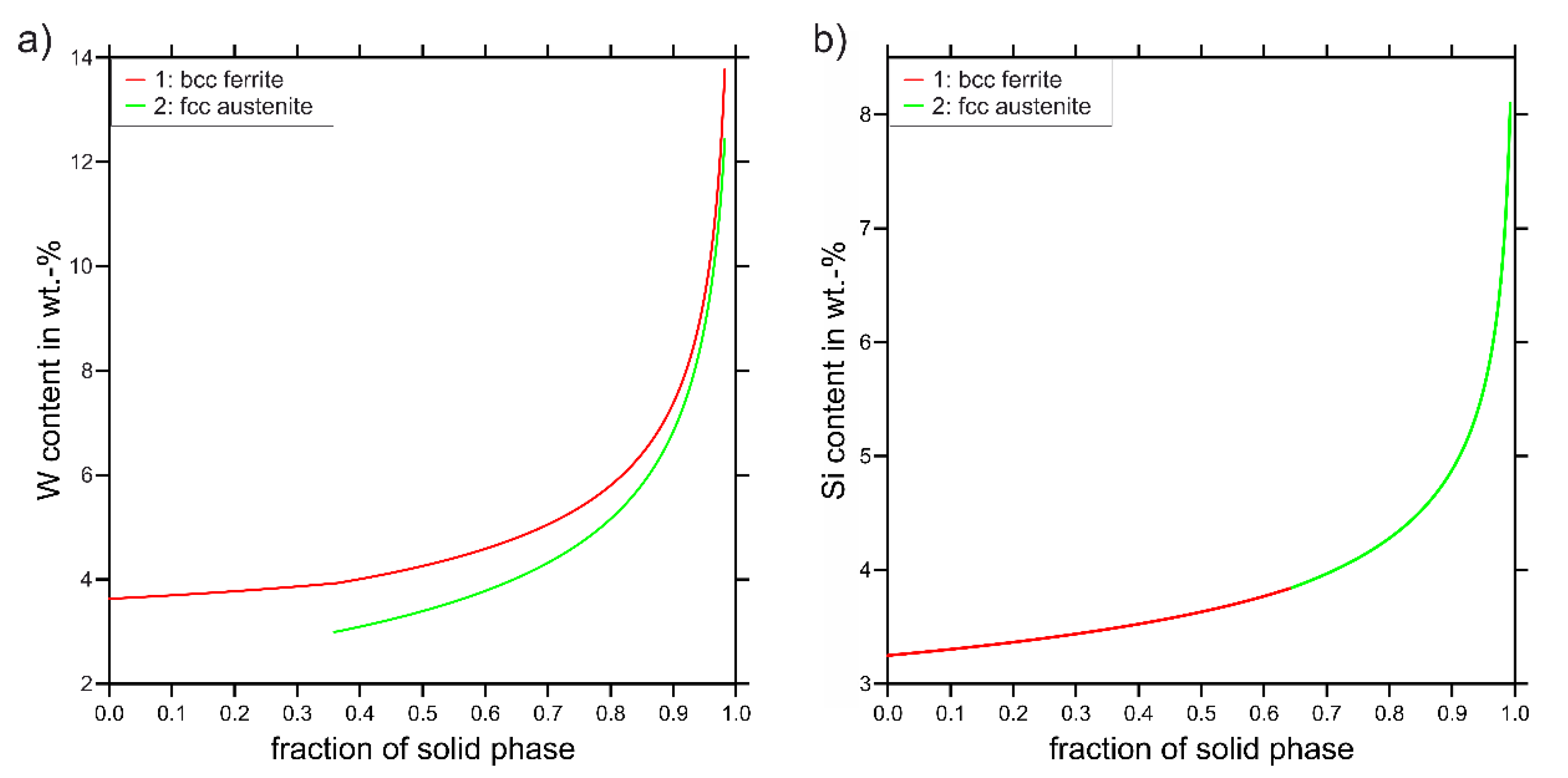
2.2. Thermodynamic Calculations

In order to design the two modified versions of the steel, X2CrNi18-9, with improved X-ray visibility of the segregation structures, thermodynamic equilibrium calculations, as well as solidification simulations with the Scheil–Gulliver model, were performed. The aim of the equilibrium calculations was to identify those elements with a distinctly high or low atomic number, significant amounts of which can be dissolved in the solid solution of the austenite during solution annealing. The subsequent solidification simulations were used to evaluate the segregation behavior of the modified alloys and to derive density profiles from the simulated segregation profiles. The calculations were performed with the Thermo-Calc software (Thermo-Calc Software AB, Solna, Sweden), version 2020b, and the thermodynamic database, TCFe10. For the solidification simulations, a starting temperature of 2000 K and a step size of 1 K were set. C and N were set as fast-diffusing elements.

2.3. Microscopy

The as-cast microstructures of the manufactured ingots were investigated by means of scanning electron microscopy and EDS. To that end, metallographic samples (15 × 15 × 10 mm) were cut from the ingots, embedded in a resin, and then ground and polished, up to a 1 µm finish. To ensure high surface quality, a final preparation step of vibratory polishing with colloidal SiO2 suspension was performed for 12 h. For the investigations, an SEM Mira 3 by Tescan (Brno, Czech Republic), equipped with an X-max 50 EDS system from Oxford Instruments (Abingdon, UK) was used. The SEM was operated with an acceleration voltage of 20 kV and a working distance of 15 mm. Backscattered electron images were taken from the samples. In order to determine the local distribution of the alloying elements, two-dimensional (2D) maps were recorded. A step size of 0.1 µm and a dwell time of 13 ms per pixel were used for the measurements. The recorded data were quantified using the AZtec software version 5.0 HF1 (Oxford Instruments, Abingdon, UK) and were then exported as ASCII datasets. The MATLAB software (The Mathworks Inc., Natick, MA, USA), version 2018a, was then used to visualize 2D element distributions and to calculate and visualize the 2D distributions of the mean atomic numbers in the solid solution. The latter were calculated using Equation (2), as suggested by Lloyd [31], using the atomic fraction, Xi, and the atomic number, Zi, of all the constituent elements.
Z ¯ = i = 1 n Z i   × X i
The examination of secondary cracks was carried out by means of light microscopy using a Leica DM6 M (Leica Microsystems GmbH, Wetzlar, Germany) microscope, equipped with a motorized stage. For the microscopic investigations, the sectioned tensile specimen was metallographically prepared by embedding in a resin bond, followed by several steps of manual grinding and polishing. In a 13.2-millimeter-long surface section of the specimen, individual micrographs were recorded and subsequently merged into one image for later analysis.

2.4. µ-CT

The CT measurements were performed using the EasyTom 160 µ-CT from RX Solutions (Chavanod, France). The tomography machine was equipped with a nanofocus X-ray generator manufactured by Hamamatsu Photonics (Hamamatsu, Japan), which was operated with acceleration voltages of between 20 kV and 160 kV and atube current of up to 200 µA. The voltage, as well as the tube current, were varied to achieve optimized parameters for the intended investigations. In order to minimize the beam-hardening artifacts, a filter with a thickness of 0.5 mm was used. Image recording was performed using a flat panel detector with an active pixel area of 1874 × 1496 pixels and a pixel size of 127 µm, operating at a frame rate of 0.5 frames per second. The angle step size for the rotation of the specimen was set to 2.5°. At each angle, ten images were recorded and averaged. In order to achieve an optimal spatial resolution, the distance between the specimen rotation axis, the tube, and the detector was adjusted in consideration of specimen geometry and image quality. The smallest possible distance between the tube and the specimen rotation axis resulted in the highest spatial resolution. By using specimen shapes with a small diameter, a voxel size of 1.29 µm could be achieved.
Three-dimensional reconstructions of the investigated specimens were created from the recorded X-ray projections using the filtered back-projection method, which is implemented in the software X-Act (RX Solutions, Chavanod, France). The reconstruction included the correction of those artifacts that were induced by focal spot drift and the geometrical inaccuracies of the µ-CT device. The software VGStudio MAX 3.2 (Volume Graphics GmbH, Heidelberg, Germany) was used to extract image slices from the reconstructed data.

2.5. Image Analysis

The secondary cracks were evaluated by determining the number of cracks per unit length of the specimen surface and by measuring the crack depth in terms of the distance between the specimen surface and the crack tip. This means that the measured crack depth represents the minimum depth of a crack. As the image resolution might not be sufficient to resolve the smallest crack tips, the true crack depth is assumed to be marginally greater. In both the light-microscopic image and the CT image slices, each crack was identified, counted, and measured manually using the public domain software ImageJ in its version 1.53f51.

3. Results and Discussion

The results collected in this study can be divided according to the overall objectives of the investigation: on the one hand, the visualization of segregation structures via CT, and on the other hand, the analysis of secondary cracks via CT. Starting with the results for the detection of segregation structures, the findings will be described and discussed separately, before both aspects are brought together in a conclusion.

3.1. Detection of Segregation Structures

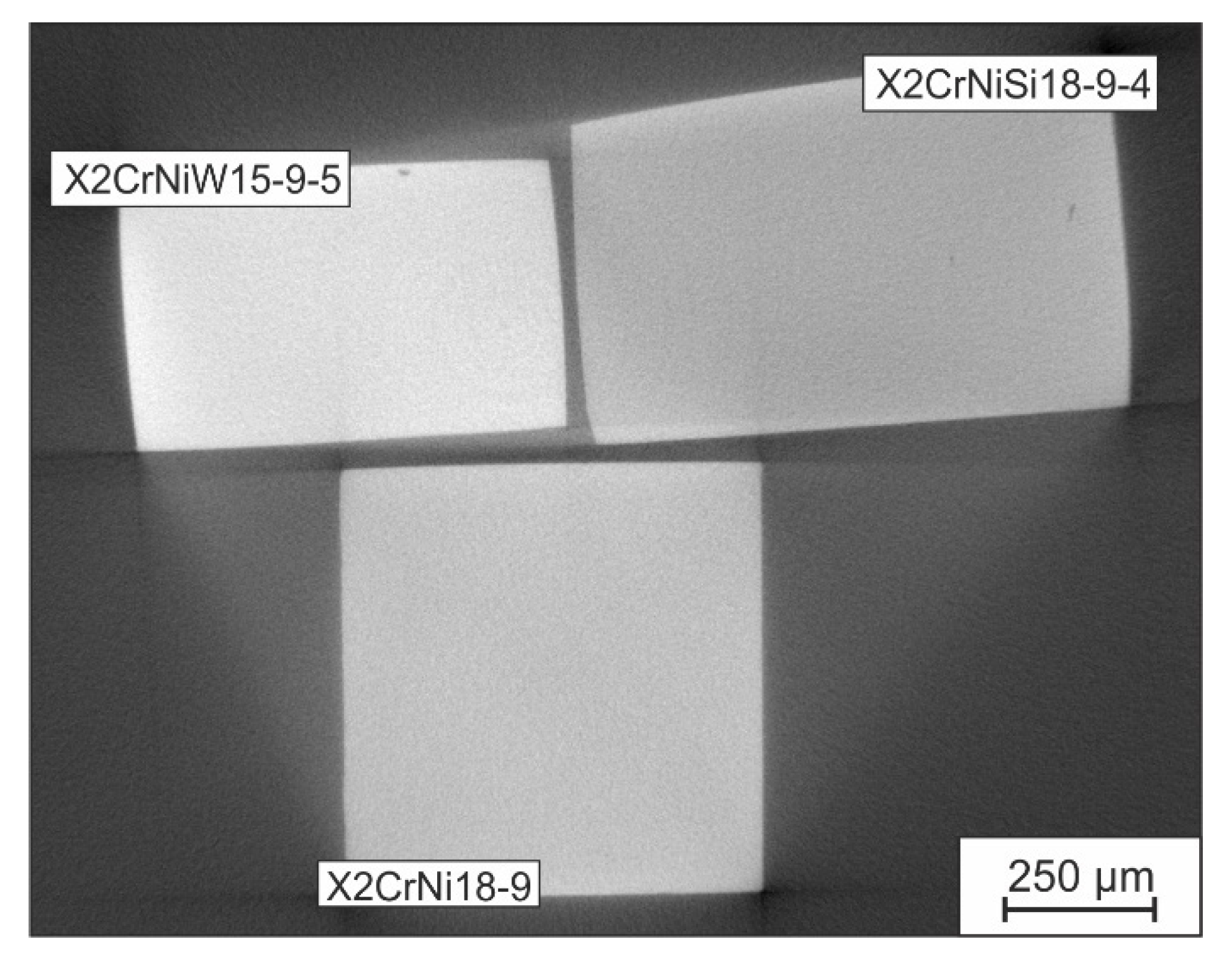
3.1.1. Design of the Model Alloys

As previously stated, in order to improve the detectability of segregation structures in austenitic CrNi steel, two model alloys doped with tracer elements were designed by employing thermodynamic calculations. For the selection of suitable tracer elements, thermodynamic calculations were carried out with a number of potential high- and low-density alloying elements. To achieve a homogeneous austenitic microstructure by solution annealing, a single-phase fcc region must be present in the phase diagram, as in the case of the X2CrNi18-9 steel (Figure 1a). The thermodynamic calculations showed that several elements, e.g., Al, Ti, Ta, and Nb, can only be added in very small quantities without stabilizing undesirable ferritic, intermetallic, or carbide phases at solution-annealing temperatures. W and Mo were identified as possible high-density tracer elements, with W being considered the more promising candidate for the later CT investigations due to its significantly higher atomic number. As with Cr, W strongly stabilizes the bcc phase [32]. To compensate for the bcc-stabilizing effect of W, the Cr content was reduced from 18 to 15 wt.-% in order to extend the fcc phase field and allow higher W contents in the fcc solid solution. The calculated phase diagram in Figure 1b reveals that more than 5 wt.-% of W can be dissolved in the fcc solid solution at 1200 °C. Thus, it can be assumed that a fully austenitic microstructure can be produced in an X2CrNiW15-9-5 steel.
As a low-density tracer element, silicon has also been identified as a suitable candidate. Despite the strong bcc stabilizing effect of Si, the thermodynamic calculations indicate that approximately 5 wt.-% of Si can be dissolved in the fcc lattice at temperatures of around 1000 °C, even without lowering the Cr content [32]. This can be seen in the calculated phase diagram depicted in Figure 1c. Accordingly, the X2CrNiSi18-9-4 steel is also considered to be qualified for manufacture with a fully austenitic microstructure.
The effects of the tracer elements on segregation-related density gradients in the considered steels were evaluated by means of solidification simulations. Figure 2a shows the density profiles of the bcc and fcc phases in each alloy, which were calculated from the segregation profiles resulting from Scheil–Gulliver solidification simulations. Figure 2b shows the corresponding fractions of the solidified phases. All three alloys feature a primary ferritic solidification, with the subsequent formation of austenite. The depicted profiles reveal that the density of the W-alloyed steel is shifted to a higher level, while the density of the Si-alloyed steel is significantly reduced, compared to the X2CrNi18-9 steel.
The reference steel, X2CrNi18-9, exhibits very small local differences in its density of roughly 0.1 g/cm3. In both modified alloys, the local differences in density are drastically increased, to approximately 0.45 g/cm3 in the case of X2CrNiW15-9-5 and to 0.5 g/cm3 in the case of X2CrNiSi18-9-4. A closer look at the density profiles of the individual phases shows that the density is subject to significant changes as soon as the solidification of the fcc phase begins. However, in the X2CrNiW15-9-5 steel, the most significant increase in density does not occur in the fcc phase but instead in the bcc phase, which continues to solidify simultaneously. In contrast, in the X2CrNiSi18-9-4 steel, the fcc phase shows a higher density gradient. With the start of solidification of the fcc phase, no more of the bcc phase solidifies in this steel. The density of the solidifying fcc phase is initially higher than in the already present bcc phase before it decreases drastically. The curve progressions indicate that the respective tracer elements accumulate in the residual melt during solidification. This assumption is supported by the respective W and Si concentrations in the solidifying phases, as illustrated in Figure 3. Figure 3a clarifies that in the X2CrNiW15-9-5 steel, W accumulates in both of the simultaneously solidifying fcc and bcc phases toward the end of the solidification process, resulting in the increasing density of both phases. In Figure 3b, it can be observed that in the X2CrNiSi18-9-4 steel, the transition from ferritic to austenitic solidification is accompanied by an increased accumulation of Si in the evolving solid phase, which is accountable for the decreasing density. The enrichment of the tracer elements toward the end of the solidification sequence, which was observed in both steels, can be considered to be a result of the low equilibrium solubility of these elements in the precipitating phases [33]. In the context of the present study, this behavior can be regarded as useful for the adjustment of local density gradients. It can be concluded that adding W or Si to the X2CrNi18-9 steel significantly impacts the average density and leads to a considerable increase in local density differences. It can therefore be assumed that the X-ray visibility of segregation structures is significantly improved in the modified alloys.

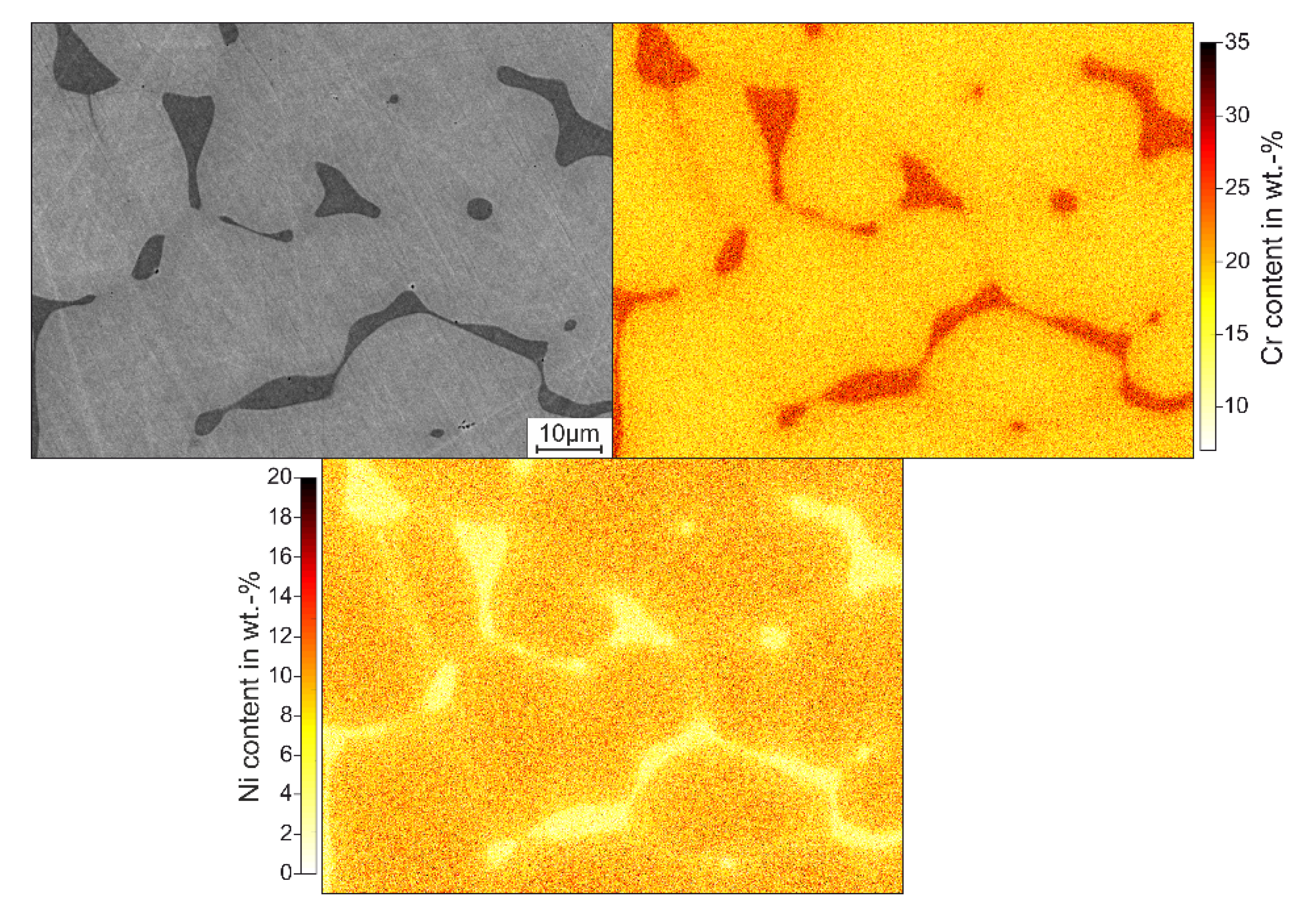
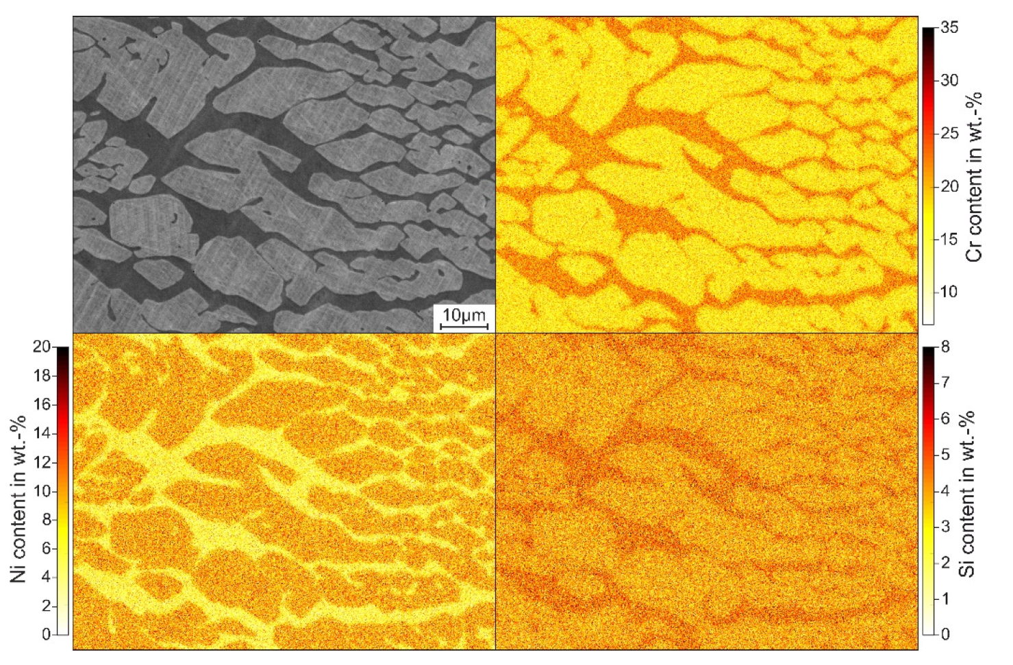
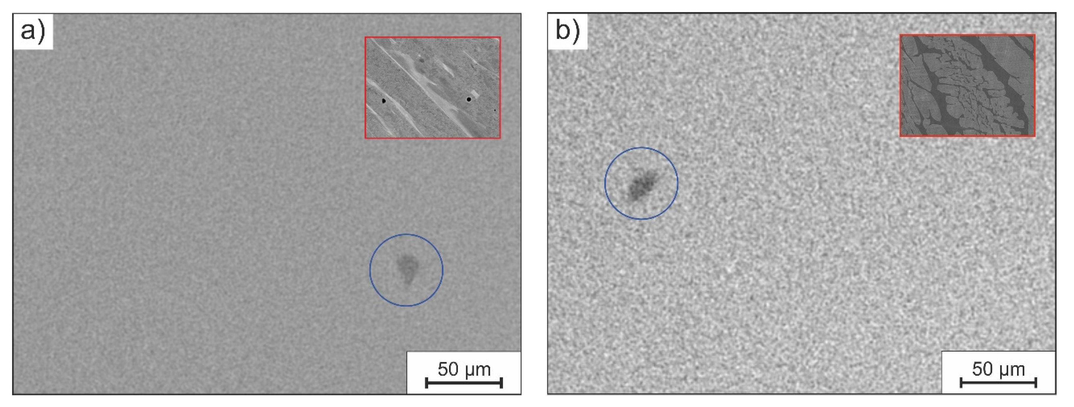
3.1.2. Two-Dimensional Investigation of the As-Cast Microstructures

The microstructures of the X2CrNi18-9, X2CrNiW15-9-5, and X2CrNiSi18-9-4 steels were investigated in the as-cast state, in order to assess the local element distributions using the conventional 2D strategy. The SEM backscatter electron (BSE) micrographs of all three alloys, presented in Figure 4, Figure 5 and Figure 6, exhibit two-phase microstructures consisting of austenite and δ-ferrite. The latter can be identified based on the illustrated element distributions, via the high Cr and low Ni contents [34]. Considering the previously shown phase diagrams (Figure 1), the δ-ferrite can be removed or at least diminished by solution annealing. However, no heat treatment was performed in this case, as this highly inhomogeneous condition is considered to provide the best conditions for CT studies.
The local element distributions in the X2CrNi18-9 steel shown in Figure 4 indicate that in addition to the previously mentioned partitioning of Cr and Ni into austenite and δ-ferrite, concentration gradients also exist within the austenite. With increasing distance from the ferritic sites, the Cr content decreases within the austenite, while the Ni content increases. This is the result of the solidification and transformation sequence during cooling. Usually, the Cr content of the primary solidifying ferrite is higher than the average Cr content of the melt, and vice versa for the Ni content. Due to the enrichment of the melt with Ni and its depletion with Cr, the Cr concentration of the further solidifying ferrite decreases, while the Ni concentration increases, until the beginning of the precipitation of the austenitic phase from the melt [35]. During the subsequent cooling, starting from the last-solidified, low-Ni ferrite, a ferrite–austenite transformation takes place, so that the concentration profiles described are present in the austenite in the as-cast state. The described tendency can also be observed in the case of the X2CrNiW15-9-5 steel (Figure 5), but not in the X2CrNiSi18-9-4 steel (Figure 6). The reason for this may be that in the latter, no significant ferrite–austenite transformation occurs during cooling.
In the X2CrNiW15-9-5 steel, the individual phases exhibit significantly different W contents, with around 4 wt.-% in the austenite and approximately 9 wt.-% in the δ-ferrite (Figure 5). The fact that no content for δ-ferrite with W at around 4 wt.-% is present in the microstructure, as indicated by the Scheil-Gulliver simulations (Figure 3), can be attributed to the transformation of δ-ferrite into austenite during the cooling of the solidified material. It is only in regions of the microstructure with particularly high W contents that the δ-ferrite is stable enough to persist until cooling to room temperature. In the X2CrNiSi18-9-4 steel, Si is enriched in the δ-ferrite, contrary to expectations based on the solidification simulations. This raises doubts regarding the accuracy of the thermodynamic calculations performed for the X2CrNiSi18-9-4 steel. Other authors also observed discrepancies between the results of the Scheil–Gulliver solidification simulations and experimental results for high-Si steel [36]. This might indicate that either the thermodynamic database or the calculation models are not designed for such unusually high Si contents. However, other authors were able to gather reliable simulation results for austenitic steels with medium Si contents [37,38].
The above-described element distributions result in inhomogeneous local distributions of the mean atomic number of the solid solution that are, according to Equation (1), highly relevant for X-ray visibility. Figure 7 illustrates the 2D distributions of the mean atomic numbers, calculated from the EDS data recorded in the sites illustrated in Figure 4, Figure 5 and Figure 6. While the atomic numbers in the X2CrNi18-9 and X2CrNiSi18-9-4 steels are lower in the δ-ferrite than in the austenite, the atomic numbers in the X2CrNiW15-9-5 steel show an opposite relationship. From the color scales, it can be seen that the X2CrNi18-9 steel has the smallest difference between the minimum and maximum mean atomic numbers, with values of between approximately 24.8 and 26 (ΔZ = 1.2). The X2CrNiW15-9-5 alloy has the highest atomic numbers, with values ranging from about 25.5 to 27.5 (ΔZ = 2), as well as the highest difference between the minimum and maximum values. The average atomic numbers in the X2CrNiSi18-9-4 alloy are the lowest, with values ranging from about 24 to 25.7 (ΔZ = 1.7). Despite the Si distribution being different from what was indicated by the solidification simulations, the actual Si distribution resulted in significantly increased local Z differences compared to the reference steel, X2CrNi18-9.

3.1.3. CT Investigations

For the CT imaging of the previously described elemental distributions, thin specimens with cross-sections of 1 × 1 mm were manufactured from the as-cast states of all three steels and were examined individually. The parameters of the CT measurements were varied, as described in Section 2.4, in order to receive optimized imaging conditions. High-resolution CT slices of the steels with the highest local Z-differences, X2CrNiW15-9-5 and X2CrNiSi18-9-4, are depicted in Figure 8. The associated measurements were made with a tube current of 100 kV. In both images, spots in dark gray tones, highlighted by the blue circles, stand out from the background noise. These spots, which reach sizes of up to 30 µm, represent those constituents of the microstructure with a low X-ray attenuation and can be classified as non-metallic inclusions [39,40]. After several measurements with different tube currents, 100 kV was identified as the voltage with which the non-metallic inclusions can be imaged most clearly in the given setup. It was, therefore, expected that this voltage would also be the most suitable for detecting other structures. In principle, better contrasts can be produced by reducing the voltage, although the image noise increases at the same time. Therefore, it is challenging to find a suitable voltage for the optimal contrast-to-noise ratio [41]. However, other structures than non-metallic inclusions that might represent element segregations or δ-ferrite are not visible in the images (Figure 8). The SEM images of the microstructure, depicted in the red boxes, illustrate the dimensions of the structures that were supposed to be visualized via CT. The δ-ferrite channels that are extended through the austenite have widths of up to about 10 µm, which is somewhat smaller than the size of the non-metallic inclusions but well above the voxel size of 1.29 µm. The fact that no such structures could be imaged is likely a result of the combination of various causes. The size ratio between δ-ferrite and voxels leads to the effect that, even in advantageous sites, only a few contiguous voxels can be completely assigned to the δ-ferrite. At the same time, there are probably only marginal differences in the X-ray contrast of austenite and δ-ferrite, combined with the comparatively high measurement noise that comes with the large magnification. Image noise might be reduced by drastically increasing the number of recorded and averaged images at each rotation angle of the specimen. However, this increases the acquisition time considerably and makes measurement impracticable.
In order to investigate the imageability of small differences in atomic number with the selected CT setup, the samples of the three steels were measured together in a CT scan. An image slice produced in this scan is illustrated in Figure 9. The image reveals that the specimens are contrasted in different grayscales, proving the impact of the different mean atomic numbers of the three steels. Table 2 lists the average 8-bit grayscale values of the three steels, extracted from the image in Figure 9, together with the respective mean atomic number, Z ¯ . The data verify the apparent correlation between atomic number and gray level, in that an increasing atomic number is associated with an increasing attenuation of X-rays, which is represented here as brighter shades. The data further demonstrates the level of difference that the atomic numbers must exhibit to produce contrast. The Z-difference of 0.6 that prevails between X2CrNi18-9 and X2CrNiSi18-9-4 is sufficient to distinguish the gray values, both visually and quantitatively, on the basis of their average values. Since the local Z-differences previously found in the microstructures of the steels are considerably larger, it can be assumed that these could not be detected by CT, mainly due to their small dimensions and a reduction in the actual resolution because of image noise [42]. It can be concluded that the resolution and signal-to-noise ratio requirements, in this case, exceeded the capabilities of the laboratory-scale CT equipment used. To achieve better results regarding the visualization of elemental segregations in 3D, a measurement setup with a synchrotron radiation source could be used in future investigations. The signal yield using synchrotron radiation usually exceeds the capabilities of laboratory instruments by a considerable margin [43,44]. Further improvements in measurement performance might be achieved by adjusting the specimen geometry or by accepting significantly prolonged measurement times.

3.2. Detection of Hydrogen-Induced Cracks

For the assessment of the X-ray visibility of hydrogen-induced cracks, the cracked specimen described in Section 2.1 was examined via light microscopy and CT. The example in Figure 10 illustrates the appearance of cracks in a light microscopic image and in a CT-slice image. Despite relatively strong image noise, the contours of the cracks can be seen clearly in the CT image. However, it becomes clear that the exact location of the crack tips is difficult to identify. Again, the maximum achievable resolution, which is reduced by the image noise, is the limiting factor for the imaging of these small-scale structures [42].
For the applicability of CT measurements in the quantification of secondary cracks, it is important to know the limitations of the imageability of cracks, resulting from the lower resolution compared to microscopic images. To estimate the resulting error in a quantitative analysis, cracks along an 11-millimeter surface section were evaluated using images from both examination methods. The results of this analysis are shown in Table 3. As expected, the lowest detectable crack depth in the CT measurements is significantly higher. The smallest cracks that were detected in the CT slices have depths of approximately 5 µm. In the light-microscopic images, cracks of approximately 2 µm in depth can also be identified. These smaller cracks are theoretically also imageable via CT, since the voxel size of 1.29 µm is sufficiently small. However, as stated above, these very small cracks are likely to be covered up by the measurement noise, as they are incorporated by very few or even single voxels. As a result of the higher detection limit for cracks in the CT images, the evaluation of the CT data yields a higher value for the mean crack depth. The measured crack densities, however, are very similar, which indicates that the size of most cracks in the specimen is above the detection limit of CT.
Regardless of the weaknesses in measuring cracks by CT, this method has the decisive advantage that image data for an arbitrary number of planes of the specimen are generated with one measurement. This opens up the possibility of evaluating the entirety of the cracks present in the specimen and not just single micrographs. This makes it possible to achieve a better statistical validation of the results. Of course, this approach requires separate, automated evaluation methods in which cracks are automatically detected and measured.

4. Conclusions

The aim of the investigations in this study was to visualize segregation structures and hydrogen-induced cracks in austenitic CrNi-type steels using CT. The following conclusions can be drawn from the results of the respective investigations of these two aspects:
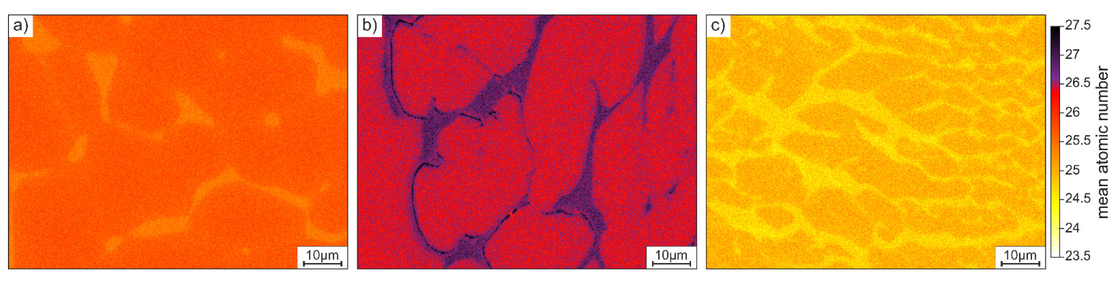
  • By modifying the alloy composition of X2CrNi18-9 with W or Si, a significant change in the X-ray attenuation can be achieved, which can be visualized via CT. Local segregation-related differences in the mean atomic number are also strongly increased by the alloy modifications and are believed to be sufficient for CT imaging. The fact that none of these structures could be visualized can most probably be attributed to their small size.
  • Hydrogen-induced cracks could be detected via CT, with the lower detection limit of the used setup being somewhat smaller than in microscopic investigations. The smallest cracks (<5 µm) were overlooked via CT. For the quantitative analysis of larger cracks, CT might serve well in the investigation of the whole volume of a specimen as it provides better statistics, compared to the microscopic investigation of single sections.
  • This study attempted to visualize the segregation structures and hydrogen-induced cracks in separate CT measurements. Since maximum resolution is the limiting factor in both aspects, the simultaneous investigation of both aspects on a suitable sample is probably possible. The prerequisite for this would presumably be larger-scale segregation structures or the use of a measurement setup allowing better imaging, e.g., by synchrotron radiation.

Author Contributions

G.E.: Conceptualization, methodology, validation, investigation, data curation, writing—original draft preparation, visualization, supervision, and funding acquisition. S.S.: Investigation, data curation, and visualization. S.B.: Conceptualization, methodology, writing—review and editing, and supervision. S.W.: Conceptualization, resources, writing—review and editing, supervision, and funding acquisition. All authors have read and agreed to the published version of the manuscript.

Funding

This research was funded by the Deutsche Forschungsgemeinschaft (DFG), grant number 456380481-WE 4436/7-1.

Institutional Review Board Statement

Not applicable.

Informed Consent Statement

Not applicable.

Data Availability Statement

The data presented in this study are available on request from the corresponding author.

Acknowledgments

The authors gratefully acknowledge the Center for Interface-Dominated High-Performance Materials (Zentrum für Grenzflächendominierte Höchstleistungswerkstoffe, ZGH) at Ruhr-University Bochum, Germany for the use of their µ-CT device, and Johannes Boes for performing the measurements.

Conflicts of Interest

The authors declare no conflict of interest.

References

  1. Birnbaum, H.K. Hydrogen Related Fracture of Metals. In Atomistics of Fracture; Latanision, R.M., Pickens, J.R., Eds.; Springer: Boston, MA, USA, 1970; ISBN 978-1-4613-3502-3. [Google Scholar]
  2. Abraham, D.P.; Altstetter, C.J. Hydrogen-enhanced localization of plasticity in an austenitic stainless steel. Metall. Trans. A 1995, 26, 2859–2871. [Google Scholar] [CrossRef]
  3. Robertson, I.M.; Tabata, T.; Wei, W.; Heubaum, F.; Birnbaum, H.K. Hydrogen embrittlement and grain boundary fracture. Scr. Metall. 1984, 18, 841–846. [Google Scholar] [CrossRef]
  4. Gavriljuk, V.G.; Shanina, B.D.; Shyvanyuk, V.N.; Teus, S.M. Hydrogen embrittlement of austenitic steels: Electron approach. Corros. Rev. 2013, 31, 33–50. [Google Scholar] [CrossRef]
  5. Rozenak, P. Effects of nitrogen on hydrogen embrittlement in AlSl type 316, 321 and 347 austenitic stainless steels. J. Mater. Sci. 1990, 25, 2532–2538. [Google Scholar] [CrossRef]
  6. San Marchi, C. Effects of alloy composition and strain hardening on tensile fracture of hydrogen-precharged type 316 stainless steels. Int. J. Hydrog. Energy 2008, 33, 889–904. [Google Scholar] [CrossRef]
  7. Zhang, L.; An, B.; Fukuyama, S.; Iijima, T.; Yokogawa, K. Characterization of hydrogen-induced crack initiation in metastable austenitic stainless steels during deformation. J. Appl. Phys. 2010, 108, 63526. [Google Scholar] [CrossRef]
  8. Gavriljuk, V.G.; Shanina, B.D.; Shyvanyuk, V.N.; Teus, S.M. Electronic effect on hydrogen brittleness of austenitic steels. J. Appl. Phys. 2010, 108, 83723. [Google Scholar] [CrossRef]
  9. Tabata, T.; Birnbaum, H.K. Direct observations of hydrogen enhanced crack propagation in iron. Scr. Metall. 1984, 18, 231–236. [Google Scholar] [CrossRef]
  10. Birnbaum, H.K. Hydrogen Embrittlement. In Encyclopedia of Materials: Science and Technology; Elsevier: Amsterdam, The Netherlands, 2001; pp. 3887–3889. [Google Scholar]
  11. Somerday, B.P.; Gangloff, R.P. (Eds.) Gaseous Hydrogen Embrittlement of Materials in Energy Technologies: Volume 1: The Problem, Its Characterisation and Effects on Particular Alloy Classes; Woodhead Publishing Ltd.: Cambridge, UK, 2012; ISBN 978-1-84569-677-1. [Google Scholar]
  12. San Marchi, C.; Michler, T.; Nibur, K.A.; Somerday, B.P. On the physical differences between tensile testing of type 304 and 316 austenitic stainless steels with internal hydrogen and in external hydrogen. Int. J. Hydrog. Energy 2010, 35, 9736–9745. [Google Scholar] [CrossRef]
  13. Michler, T.; Naumann, J. Microstructural aspects upon hydrogen environment embrittlement of various bcc steels. Int. J. Hydrog. Energy 2010, 35, 821–832. [Google Scholar] [CrossRef]
  14. Perng, T.P.; Altstetter, C.J. Comparison of hydrogen gas embrittlement of austenitic and ferritic stainless steels. Metall. Trans. A 1987, 18, 123–134. [Google Scholar] [CrossRef]
  15. Holzworth, M.L. Hydrogen Embrittlement of Type 304L Stainless Steel. Corrosion 1969, 25, 107–115. [Google Scholar] [CrossRef]
  16. Inoue, A.; Hosoya, Y.; Masumoto, T. The Effect of Hydrogen on Crack Propagation Behavior and Microstructures around Cracks in Austenitic Stainless Steels. ISIJ Int. 1979, 19, 170–178. [Google Scholar] [CrossRef]
  17. Michler, T.; Lee, Y.; Gangloff, R.P.; Naumann, J. Influence of macro segregation on hydrogen environment embrittlement of SUS 316L stainless steel. Int. J. Hydrog. Energy 2009, 34, 3201–3209. [Google Scholar] [CrossRef]
  18. Weber, S.; Martin, M.; Theisen, W. Impact of heat treatment on the mechanical properties of AISI 304L austenitic stainless steel in high-pressure hydrogen gas. J. Mater. Sci. 2012, 47, 6095–6107. [Google Scholar] [CrossRef]
  19. Egels, G.; Mujica Roncery, L.; Fussik, R.; Theisen, W.; Weber, S. Impact of chemical inhomogeneities on local material properties and hydrogen environment embrittlement in AISI 304L steels. Int. J. Hydrog. Energy 2018, 43, 5206–5216. [Google Scholar] [CrossRef]
  20. Kumar, B.S.; Kain, V.; Singh, M.; Vishwanadh, B. Influence of hydrogen on mechanical properties and fracture of tempered 13 wt% Cr martensitic stainless steel. Mater. Sci. Eng. A 2017, 700, 140–151. [Google Scholar] [CrossRef]
  21. Zhang, L.; Wen, M.; Imade, M.; Fukuyama, S.; Yokogawa, K. Effect of nickel equivalent on hydrogen gas embrittlement of austenitic stainless steels based on type 316 at low temperatures. Acta Mater. 2008, 56, 3414–3421. [Google Scholar] [CrossRef]
  22. Laureys, A.; Depover, T.; Petrov, R.; Verbeken, K. Microstructural Characterization of Hydrogen Induced Cracking in TRIP Steels by EBSD. AMR 2014, 922, 412–417. [Google Scholar] [CrossRef]
  23. Wilson-Heid, A.E.; Novak, T.C.; Beese, A.M. Characterization of the Effects of Internal Pores on Tensile Properties of Additively Manufactured Austenitic Stainless Steel 316L. Exp. Mech. 2019, 59, 793–804. [Google Scholar] [CrossRef]
  24. Cui, L.; Lei, X.; Zhang, L.; Zhang, Y.; Yang, W.; Gao, Y.; Liu, Y.; Liu, N. Three-Dimensional Characterization of Defects in Continuous Casting Blooms of Heavy Rail Steel Using X-ray Computed Tomography. Metall. Mater. Trans. B 2021, 52, 2327–2340. [Google Scholar] [CrossRef]
  25. Harrer, B.; Kastner, J.; Winkler, W.; Degischer, H.P. On the Detection of Inhomogeneities in Steel by Computed Tomography. In Proceedings of the 17th World Conference on Nondestructive Testing, Shanghai, China, 25–28 October 2008. [Google Scholar]
  26. Connolly, B.J.; Horner, D.A.; Fox, S.J.; Davenport, A.J.; Padovani, C.; Zhou, S.; Turnbull, A.; Preuss, M.; Stevens, N.P.; Marrow, T.J.; et al. X-ray microtomography studies of localised corrosion and transitions to stress corrosion cracking. Mater. Sci. Technol. 2006, 22, 1076–1085. [Google Scholar] [CrossRef]
  27. Marrow, T.J.; Steuwer, A.; Mohammed, F.; Engelberg, D.; Sarwar, M. Measurement of crack bridging stresses in environment-assisted cracking of duplex stainless by synchrotron diffraction. Fat Frac. Eng. Mat. Struct. 2006, 29, 464–471. [Google Scholar] [CrossRef]
  28. Marrow, T.J.; Babout, L.; Connolly, B.J.; Engelberg, D.; Johnson, G.; Buffiere, J.-Y.; Withers, P.J.; Newman, R.C. High-resolution, in-situ, tomographic observations of stress corrosion cracking. In Environment-Induced Cracking of Materials; Elsevier: Amsterdam, The Netherlands, 2008; pp. 439–447. ISBN 9780080446356. [Google Scholar]
  29. King, A.; Ludwig, W.; Engelberg, D.; Marrow, T.J. Diffraction contrast tomography for the study of polycrystalline stainless steel microstructures and stress corrosion cracking. Rev. Metall. 2011, 108, 47–50. [Google Scholar] [CrossRef]
  30. Lusic, H.; Grinstaff, M.W. X-ray-computed tomography contrast agents. Chem. Rev. 2013, 113, 1641–1666. [Google Scholar] [CrossRef] [Green Version]
  31. Lloyd, G.E. Atomic number and crystallographic contrast images with the SEM: A review of backscattered electron techniques. Mineral. Mag. 1987, 51, 3–19. [Google Scholar] [CrossRef] [Green Version]
  32. Raghavan, V.; Antia, D.P. The chromium equivalents of selected elements in austenitic stainless steels. Metall. Trans. A 1994, 25, 2675–2681. [Google Scholar] [CrossRef]
  33. Won, Y.-M.; Thomas, B.G. Simple model of microsegregation during solidification of steels. Metall. Trans. A 2001, 32, 1755–1767. [Google Scholar] [CrossRef]
  34. Wegrzyn, T. Delta ferrite in stainless steel weld metals. Weld. Int. 1992, 6, 690–694. [Google Scholar] [CrossRef]
  35. Kerr, H.W.; Kurz, W. Solidification of peritectic alloys. Int. Mater. Rev. 1996, 41, 129–164. [Google Scholar] [CrossRef]
  36. Aranda Villada, V.A.; García Hinojosa, J.A.; Cruz Mejía, H.; Balandra Aranzueta, A.A.; González, F.M.G.; Houbaert, Y. Study of the Macrosegregation of Silicon in Steels for Electrical Applications. MRS Proc. 2012, 1373, 412. [Google Scholar] [CrossRef]
  37. Weber, S.; Martin, M.; Theisen, W. Lean-alloyed austenitic stainless steel with high resistance against hydrogen environment embrittlement. Mater. Sci. Eng. A 2011, 528, 7688–7695. [Google Scholar] [CrossRef]
  38. Curtze, S.; Kuokkala, V.-T.; Oikari, A.; Talonen, J.; Hänninen, H. Thermodynamic modeling of the stacking fault energy of austenitic steels. Acta Mater. 2011, 59, 1068–1076. [Google Scholar] [CrossRef]
  39. Tian, L.; Liu, L.; Ma, B.; Zaïri, F.; Ding, N.; Guo, W.; Xu, N.; Xu, H.; Zhang, M. Evaluation of maximum non-metallic inclusion sizes in steel by statistics of extreme values method based on Micro-CT imaging. Metall. Res. Technol. 2022, 119, 202. [Google Scholar] [CrossRef]
  40. Shang, Z.; Li, T.; Yang, S.; Yan, J.; Guo, H. Three-dimensional characterization of typical inclusions in steel by X-ray Micro-CT. J. Mater. Res. Technol. 2020, 9, 3686–3698. [Google Scholar] [CrossRef]
  41. Gulliksrud, K.; Stokke, C.; Martinsen, A.C.T. How to measure CT image quality: Variations in CT-numbers, uniformity and low contrast resolution for a CT quality assurance phantom. Phys. Med. 2014, 30, 521–526. [Google Scholar] [CrossRef]
  42. Goldman, L.W. Principles of CT: Radiation dose and image quality. J. Nucl. Med. Tsechnol. 2007, 35, 213–225. [Google Scholar] [CrossRef] [Green Version]
  43. Brunke, O.; Neuser, E.; Suppes, A. High resolution industrial CT systems: Advances and comparison with synchrotron-based CT. In Proceedings of the Internal Symposium on Digital Industrial Radiology and Computed Tomography, Berlin, Germany, 20–22 June 2011; pp. 20–22. [Google Scholar]
  44. Mayo, S.C.; Stevenson, A.W.; Wilkins, S.W. In-Line Phase-Contrast X-ray Imaging and Tomography for Materials Science. Materials 2012, 5, 937–965. [Google Scholar] [CrossRef]
Figure 1. Thermodynamically calculated phase diagrams of the steels: (a) X2CrNi18-9, (b) X2CrNiW15-9-5, and (c) X2CrNiSi18-9-4 (Thermo-Calc 2020b, TCFe10 database).
Hydrogen 04 00005 g001
Figure 2. Results derived from the Scheil–Gulliver solidification simulations (Thermo-Calc 2020b, TCFe10 database). (a) The density profiles of both solidifying phases in each steel; (b) the corresponding fractions of the solidified phases.
Hydrogen 04 00005 g002
Figure 3. Element concentrations in the fcc and bcc phases, derived from Scheil–Gulliver solidification simulations. (a) W in the X2CrNiW15-9-5 steel and (b) Si in the X2CrNiSi18-9-4 steel (Thermo-Calc 2020b, TCFe10 database).
Hydrogen 04 00005 g003
Figure 4. SEM-BSE micrograph and the local element concentrations of Cr and Ni in the X2CrNi18-9 steel.
Hydrogen 04 00005 g004
Figure 5. SEM-BSE micrograph and the local element concentrations of Cr and Ni in the X2CrNiW15-9-5 steel.
Hydrogen 04 00005 g005
Figure 6. SEM-BSE micrograph and the local element concentrations of Cr and Ni in the X2CrNiSi18-9-4 steel.
Hydrogen 04 00005 g006
Figure 7. Distribution of the mean atomic number in the microstructure of (a) X2CrNi18-9, (b) X2CrNiW15-9-5, and (c) X2CrNiSi18-9-4.
Hydrogen 04 00005 g007
Figure 8. CT slices of the steels: (a) X2CrNiW15-9-5; (b) X2CrNiSi18-9-4. Blue circles highlight the non-metallic inclusions. The red boxes contain SEM images of each steel’s microstructure for comparison.
Hydrogen 04 00005 g008
Figure 9. The CT slice image with specimens of the X2CrNi18-9X2CrNiW15-9-5 and X2CrNiSi18-9-4 steels, exhibiting different gray values due to different X-ray attenuation.
Hydrogen 04 00005 g009
Figure 10. The appearance of secondary cracks in the X2CrNi18-9 steel in (a) a light microscopic image and (b) a CT-slice image.
Hydrogen 04 00005 g010
Table 1. Chemical composition of the investigated steels, shown as a mass percentage. Values were measured by optical emission spectroscopy.
AlloyCSiMnCrNiMoNW
X2CrNi18-90.0150.711.9417.608.500.300.050-
X2CrNiW15-9-50.0080.532.0414.788.660.020.0144.47
X2CrNiSi18-9-40.0054.112.0417.618.490.020.015-
Table 2. Mean atomic numbers, calculated from the measured compositions listed in Table 1, and average grayscale values extracted from the CT slice in Figure 9.
Alloy Z ¯ Average 8-Bit Grayscale Value
X2CrNi18-925.5169
X2CrNiW15-9-526.4210
X2CrNiSi18-9-424.9140
Table 3. Characteristics of secondary cracks in an 11-millimeter-long surface section of the cracked specimen.
MethodΣ CracksCrack Density (mm−1)Mean Depth (mm)Min. Depth (mm)
Light microscopy524.718.0 ± 10.11.9
CT544.922.5 ± 15.15.0
Disclaimer/Publisher’s Note: The statements, opinions and data contained in all publications are solely those of the individual author(s) and contributor(s) and not of MDPI and/or the editor(s). MDPI and/or the editor(s) disclaim responsibility for any injury to people or property resulting from any ideas, methods, instructions or products referred to in the content.

