Article

Distributional Trends in the Generation and End-Use Sector of Low-Carbon Hydrogen Plants

1
School of Mathematics and Statistics, University of Melbourne, Melbourne, VIC 3010, Australia
2
Beijing Institute of Mathematical Sciences and Applications, Tsinghua University, Beijing 101408, China
*
Author to whom correspondence should be addressed.
These authors contributed equally to this work.
Hydrogen 2023, 4(1), 174-189; https://doi.org/10.3390/hydrogen4010012
Submission received: 13 January 2023 / Revised: 23 February 2023 / Accepted: 27 February 2023 / Published: 2 March 2023
(This article belongs to the Special Issue Feature Papers in Hydrogen (Volume 2))

Abstract

:
This paper uses established and recently introduced methods from the applied mathematics and statistics literature to study trends in the end-use sector and the capacity of low-carbon hydrogen projects in recent and upcoming decades. First, we examine distributions in plants over time for various end-use sectors and classify them according to metric discrepancy, observing clear similarity across all industry sectors. Next, we compare the distribution of usage sectors between different continents and examine the changes in sector distribution over time. Finally, we judiciously apply several regression models to analyse the association between various predictors and the capacity of global hydrogen projects. Across our experiments, we see a welcome exponential growth in the capacity of zero-carbon hydrogen plants and significant growth of new and planned hydrogen plants in the 2020’s across every sector.

1. Introduction

Hydrogen has great potential as an alternative fuel source to existing fossil fuels and may play a role in the world’s coordinated attempt to reach net-zero carbon emissions during this century. Hydrogen production has already been used for numerous purposes, including production of liquid fuels, water, and space heating; direct injection into the gas grid; transport; and other industrial applications. Unlike petrol or natural gas, the combustion of hydrogen does not produce any greenhouse gas (GHG) emissions, which have a role in anthropogenic global warming. Hydrogen in its molecular form ( H 2 gas) does not exist naturally on Earth; it must be synthesised via a variety of different procedures.
The production of hydrogen is classified by colours according to its mode of preparation and associated emissions. “Green hydrogen” refers to production techniques that do not generate any GHG emissions, the most desirable outcome from a sustainability perspective. Typically, green hydrogen plants use renewable sources of energy (such as solar) to extract hydrogen via the electrolysis of water; the acquired hydrogen may then be stored and subsequently used for numerous applications. Black, brown, and grey hydrogen refer to production techniques that use black coal, brown coal, and natural gas, respectively, and are increasingly obsolete and costly energy sources with considerable amounts of emissions and harmful byproducts [1]. Blue hydrogen is a middle ground, defined as the production of hydrogen using fossil fuels followed by carbon capture and storage (CSS). This is not a truly zero-emissions process, as only a proportion of all generated GHGs can be captured, and harmful byproducts may remain.
With the increasing global interest in alternative energy sources in recent years, a great deal of research has focused on the viability and underlying science of hydrogen production. Early research into hydrogen fuel cells dates back several decades [2,3,4]. Since then, research on hydrogen production has been substantial: [5,6] each provided a review article on different electrolysis technologies, [7] detailed alkaline electrolysis (ALK), and [8,9,10] described successive advances in proton exchange membrane electrolysis (PEM). Reference [11] compared and contrasted ALK and PEM in detail.
More recent research has explored sophisticated means for integrating different renewable energy sources. In [12], the authors explored the use of geothermic energy to power electrolysis, and [13] investigated the use of micro-organisms (biocatalysed electrolysis). Then, [14] discussed further advances in such microbial electrolysis cells. More recently, [15] described how electronic waste may be used to generate metallic components for a process called “chemical looping reforming”.
There have also been many technological advances to enhance the efficiency of hydrogen production, both novel and incremental. In [16], the authors examined numerous means to reduce energy consumption during electrolysis. In [17], the authors compared the efficiency of different electrodes, with further advances made by [18]. In particular, [19] analysed electrode overpotential during ALK electrolysis production, whereas [20] explored optimal configurations of electrolysis under different conditions. In [21], the authors investigated state-of-the-art electrocatalysts, and [22] analysed the use of hybrid structures for increasingly efficient water electrolysis, combining both morphological features and electrochemical properties, whereas various researchers have studied other cutting-edge catalysts [23,24,25,26,27]. Numerous advances in blue hydrogen plants have also been made, including pyrolysis of plastic [28] and catalytic decomposition of methane [29] and other hydrocarbons [30]. Finally, numerous articles have examined different means for transportation and storage of hydrogen, an essential component of its widespread use [31,32,33,34].
In addition, numerous articles have taken a geopolitical focus, analysing both the policy environment and natural resources of various countries and their suitability for hydrogen production plants. Different papers have investigated the significant variability in countries’ adoption of hydrogen technologies, including in the United States [35], the United Kingdom [36], China [37], South Korea [36], the Philippines [38], Mexico [39], Morocco [40], and across the European Union [41]. Our previous work analysed the geographic rollout of low-carbon plants across different continents [42]. Finally, numerous authors have discussed the end-use sectors [43,44] or points of end-use [45] hydrogen energy usage, including [46], who comprehensively reviewed the same low-carbon plants we mathematically analyse.
Whereas the existing literature has been more technological or geopolitical in focus, our paper is a mathematical study of trends in the rollout and prevalence of low-carbon hydrogen plants (green and blue) with a focus on the end-use sector. We make use of time series analysis and metrics that have been extensively applied to various fields such as epidemiology [47,48,49,50,51,52,53], environmental sciences [54,55,56], finance [57,58,59,60,61,62,63,64,65,66], cryptocurrencies [67,68,69,70,71], crime [72,73,74] and other fields [75,76,77,78,79]. We are unaware of any instance where time series or distance analysis has been applied to the rollout of hydrogen plants over time and by the end-use sector. We study the changing usage and energy capacity of low-carbon hydrogen plants over time, with a particular interest in the increasing potential of green hydrogen plants, which emit zero carbon. Our main finding is promising: an exponential increase in the capacity of green plants over time, regardless of usage sector, and a dramatic closing of the gap between the capacity of green and non-green plants.

2. Data

All data analysed in this paper are drawn from the International Energy Agency (IEA) [80] and consist of plants built in (or projected to be built in) 1975–2043. This dataset records all low-carbon hydrogen plants, namely either green, zero emissions, or blue, incorporating fossil fuels and carbon capture and storage (CSS), as discussed in Section 1. We will refer to blue hydrogen plants as “Fossil” throughout the manuscript to highlight this distinction. The dataset contains four different technologies of green plants: alkaline electrolysis (ALK), proton exchange membrane electrolysis (PEM), solid oxide electrolysis cells (SOEC), and other electrolysis. The technologies of blue plants are coal gasification, natural gas reforming, and oil-based processes, in each case followed by CSS. Throughout the paper, we aggregate the four green electrolysis technologies and the three blue CSS production methods to classify each plant as green or blue/fossil. We also make use of the IEA estimated zero-carbon hydrogen capacity, measured in nm 3 /h of hydrogen for each plant. This is either quoted directly from the plant or estimated according to the stated power consumption of the plant and its technology. It is a measure of how much hydrogen the plant produces (or will produce upon completion).
The most important aspect of the dataset we analyse is the end-use sector of each plant. These are: refining (oil refining), ammonia (ammonia production), methanol (methanol production), iron and steel (steelmaking and other high-temperature iron processes), other industry (other high-temperature heat industrial applications), mobility (use in vehicles), power (use in the supply of power to the electricity grid), grid injection (injection of hydrogen into the natural gas grid), CHP (combined heat and power fuel cells), domestic heat (water and space heating), biofuels (biofuel production), synfuels (synthetic liquid fuels other than methanol), CH4 grid injection (injection of synthetic methane into the gas grid), and CH4 mobility (use of synthetic methane in vehicles). A small number of plants have more than one end-use sector, but the majority have only one.

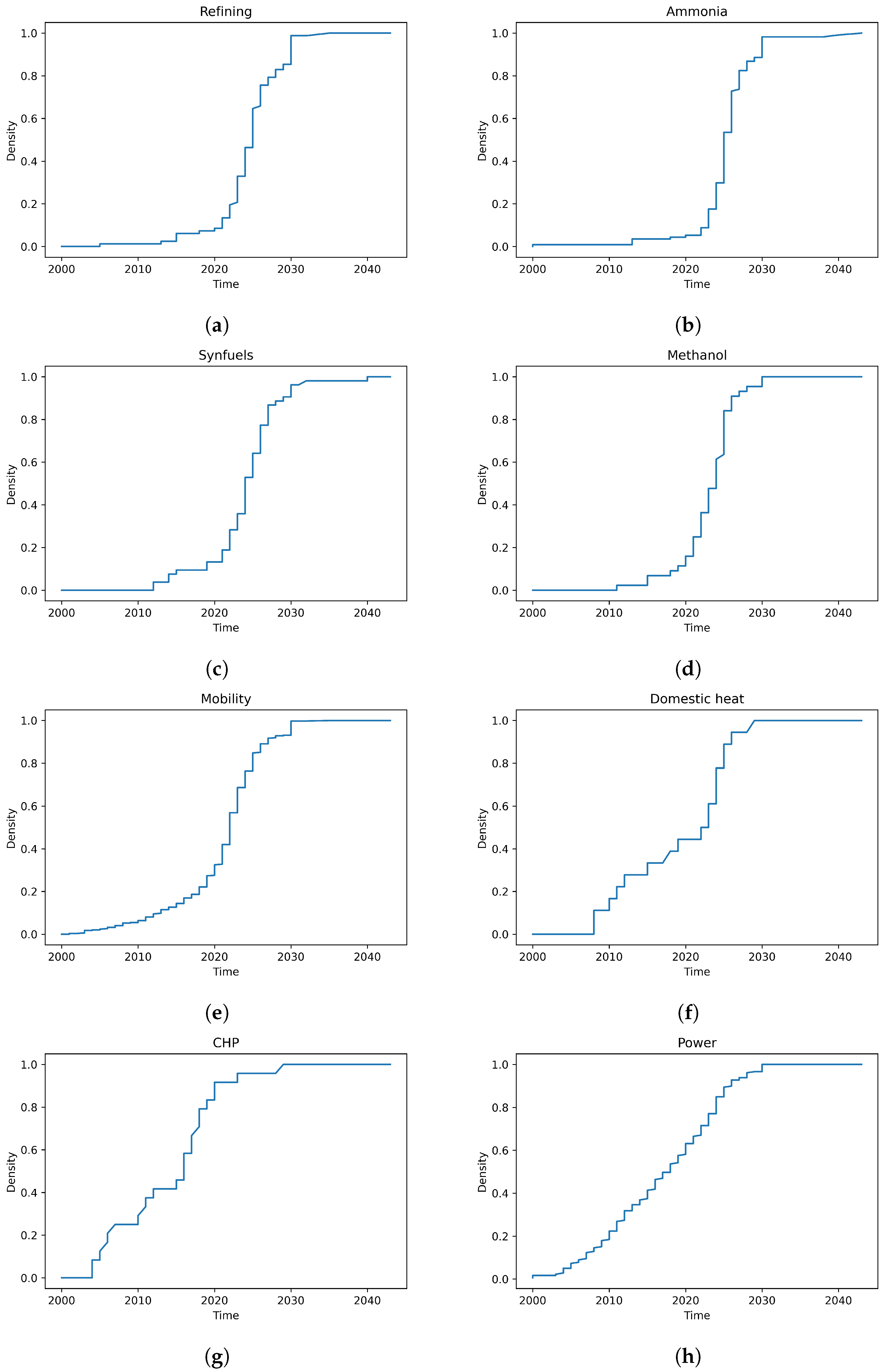
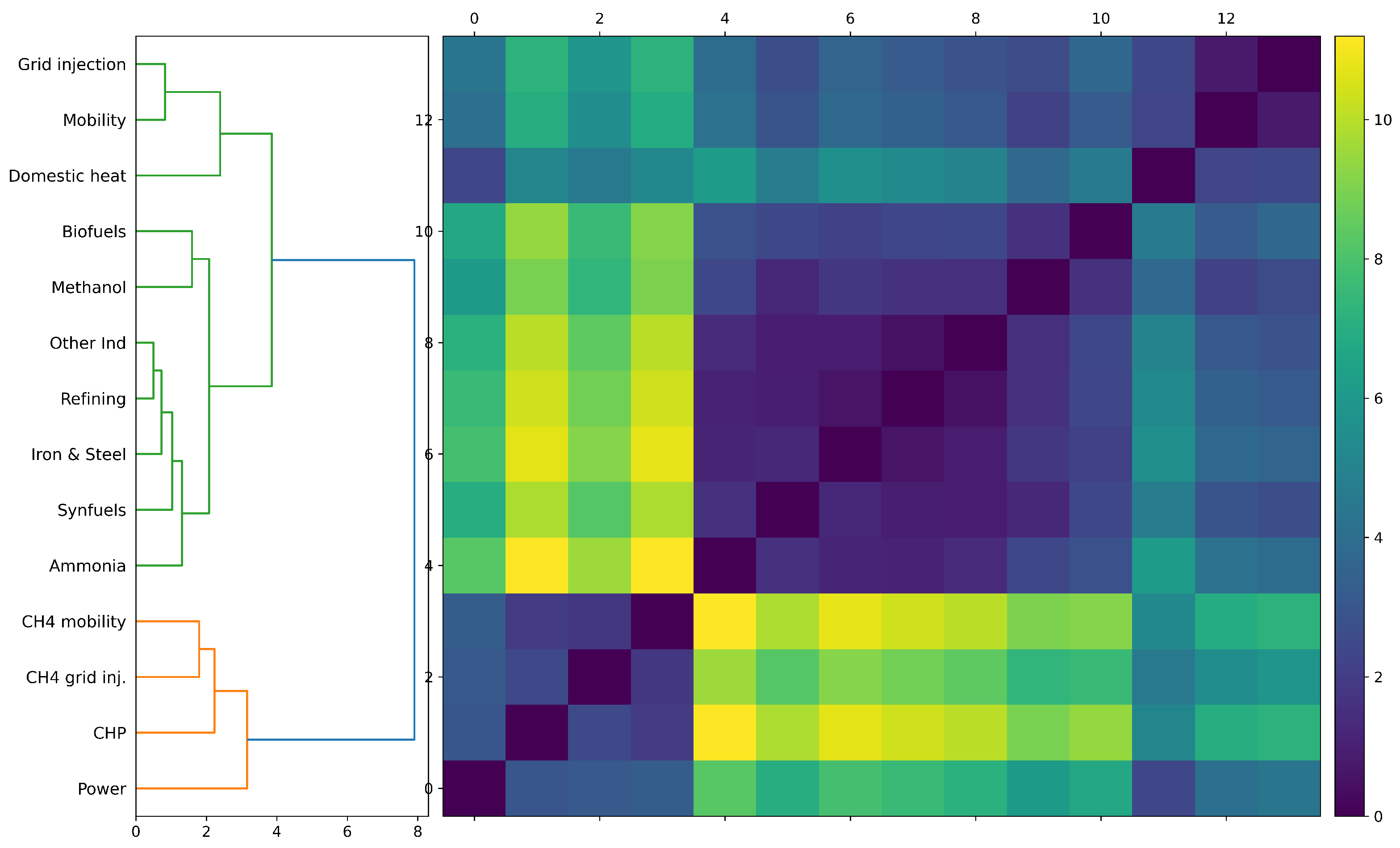
3. Distributions of End-Use Sector Over Time

In this section, we study the evolution of the propagation of low-carbon hydrogen plants for each sector and investigate the similarities in these trends. Our primary mathematical object of study is the cumulative distribution function (CDF) F S ( t ) of number of plants over time for each end-use sector S. This is defined as the proportion of plants with end-use sector S indexed with time t out of all plants with that sector. As such, it is a non-decreasing function from 0 to 1. We remark that a small number of plants have more than one usage sector, and thus will contribute to more than one CDF. This is no problem for our analysis. The temporal CDFs for eight sectors S are displayed in Figure 1. As only four plants in total are indexed before t = 2000 , we exclude these from our figures.
In Figure 2, we perform hierarchical clustering on these figures using the L 1 metric between these CDFs, defined as
d ( S 1 , S 2 ) = F S 1 F S 2 = t | F S 1 ( t ) F S 2 ( t ) | .
As all CDFs take comparable values between 0 and 1, it is appropriate to directly compare them as such.
Hierarchical clustering [81,82] is an iterative clustering technique that seeks to build a hierarchy of similarity between elements where there is some way to measure distance between them. In this case, our elements are the cumulative distribution functions equipped with the distance above. This is opposed to a technique such as k-means, which ultimately specifies k discrete groupings of elements. Hierarchical clustering is either agglomerative, where each element (CDF in our case) begins in its own cluster and branches between them are successively built, or divisive, where all elements begin in one cluster and are successively split. The results of hierarchical clustering are commonly displayed in dendrograms, which resemble branching trees. In this paper, we implement agglomerative hierarchical clustering with the average linkage method [83]. Figure 2 reveals numerous similarities and differences in the temporal distributions of new plants, which can also be seen in Figure 1.
Examining Figure 2, there is a dominant cluster of considerable similarity consisting of seven usage sectors: refining (Figure 1a), ammonia (Figure 1b), synfuels (Figure 1c), iron and steel, and other industry all occupy a subcluster of extreme similarity, while biofuels and methanol (Figure 1d) are deemed to be nearby. Curiously, all seven of these end-use sectors comprise industrial applications. Examining the plots in Figure 1, we can see these sectors’ temporal distributions are dominated by plants to be built in 2020–2030, with a smaller number in the 2010’s. Next, there is a moderately similar cluster consisting of mobility, grid injection and domestic heat. The first two, as represented by mobility (Figure 1e) have a very similar concave shape with a gradually increasing number of plants from 2000 to the 2020’s, while domestic heat (Figure 1f) features slightly more activity in the 2010’s. These three sectors reflect uses of hydrogen production that more directly service regular consumers.
Next, there are some detected outliers. CHP (Figure 1g), CH4 mobility, and CH4 grid injection all share a similar shape, exhibiting a growth in plants earlier relative to all other sectors. The most prominent outlier is power (Figure 1h), with a highly uniform growth in new plants from 2000 to 2030 observed in no other sector. Indeed, power has been one of the most consistently popular uses of hydrogen production since its inception, and this is reflected in the consistent and ongoing construction of new plants in this sector.

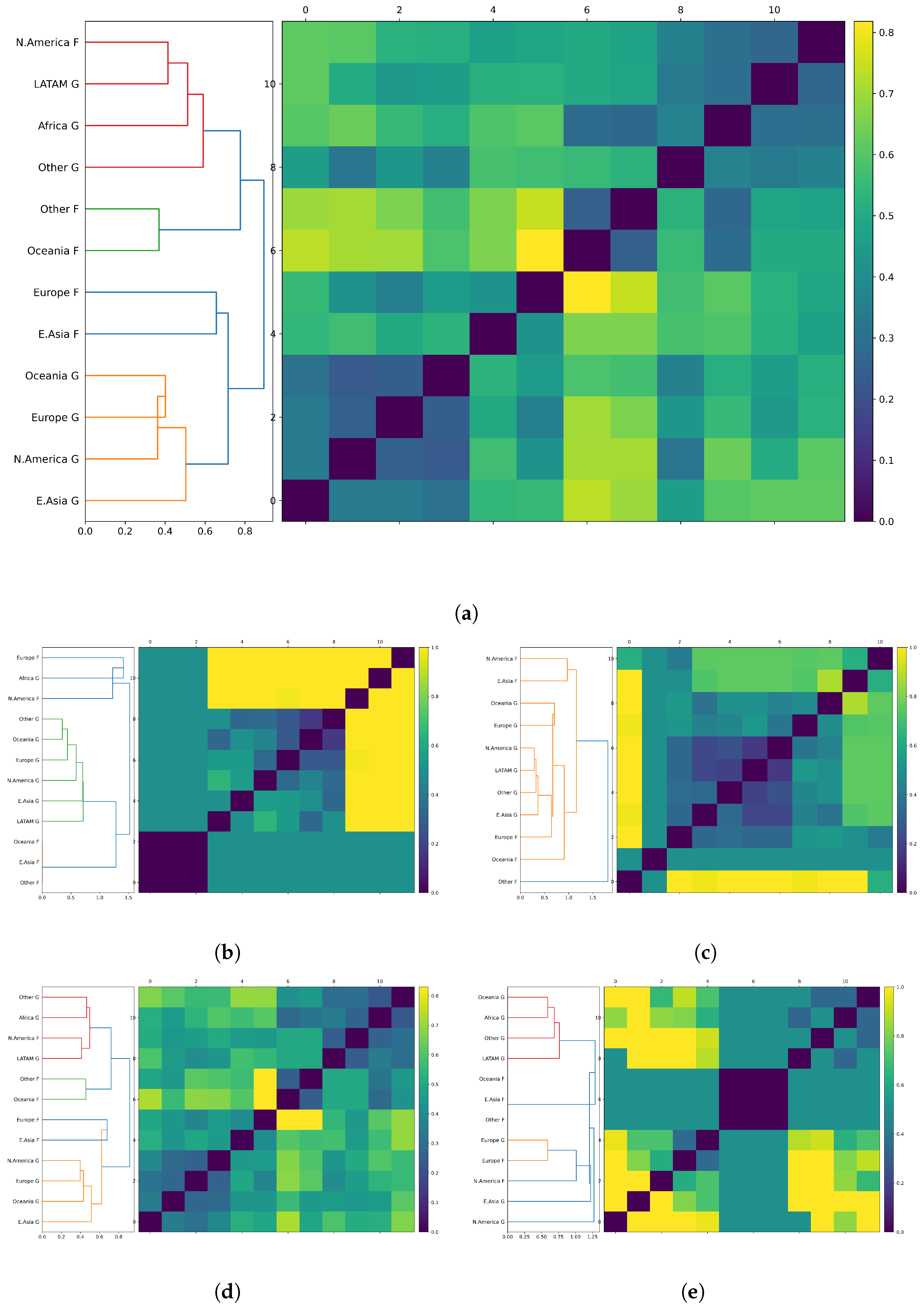
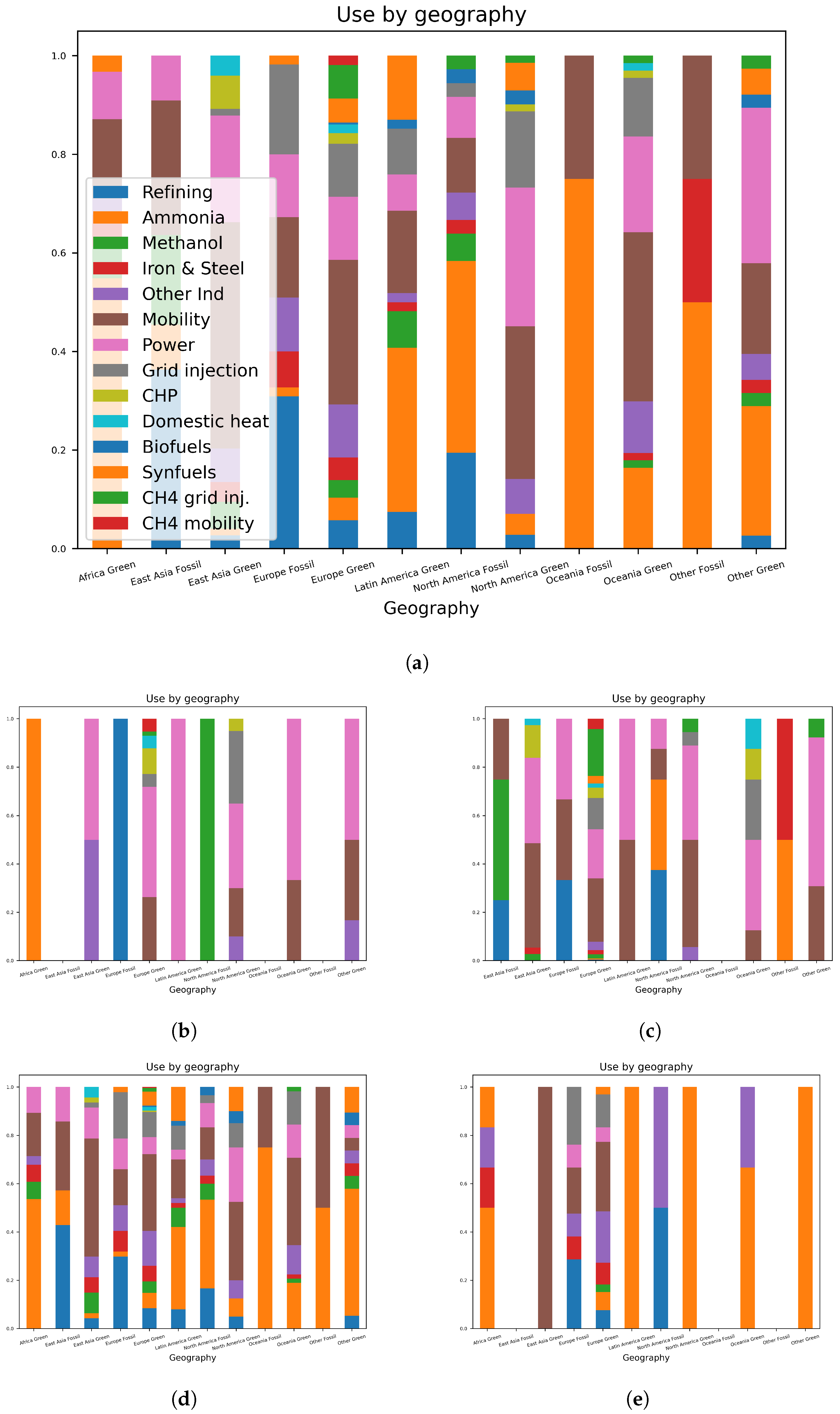
4. Usage Distributions

In this section, we investigate the distribution of plants across different sectors, focusing on each continent of location as well as green vs. blue/fossil technology. For each plant in our dataset, the location is recorded as either a country of location or continent. Thus, we first collate the plants on a continent-by-continent basis. We divide plants into seven continental and/or geopolitical regions as follows: Europe, North America (the United States and Canada), Latin America (including Mexico), Oceania, East Asia (China, Japan and Korea), Africa, and other (plants from elsewhere in Asia and the Middle East). We select these regions to combine countries according to both geographic proximity, political relations, and economic development. Next, we divide every plant up according to groups that specify both a continental region and whether the technology is green or blue/fossil. For example, we group all green European plants, or all East Asian fossil plants. There are no African fossil or Latin American fossil plants in our dataset, so this leaves 12 different continental/technological groupings G.
For each group G and end-use sector S, let p S ( G ) be the proportion of plants devoted to end-use sector S from that group, as a fraction of all the plants in the group (counting a plant multiple times if it has multiple sectors). This forms a probability vector p ( G ) R 14 of length 14. Some plants may have more than one use sector; this is fine. In those cases, a plant’s multiple sectors are counted each time in the different coefficients of p S ( G ) and also in the denominator. For example, if a group R contained just one plant with two usage sectors, say refining and ammonia, then the vector p ( R ) would be the vector ( 1 2 , 1 2 , 0 , 0 , . . . , 0 ) R 14 .
Analogously, let p ( H ) be the usage sector distribution vector for a different continental/technological group of plants H. Now we may define a distance between two distributions of usage sectors as h:
d ( G , H ) = p ( G ) p ( H ) 1 = 1 2 S | p S ( G ) p S ( H ) | .
where the sum is taken over all 14 sectors S. This has the property that d ( G , H ) = 0 if and only if groups G and H have an identical distribution of usages, again allowing multiple end-use sectors in some plants. Furthermore, d ( G , H ) 1 is the maximal possible distance, with equality if and only if the usage distributions are disjoint, with no usage sectors in common at all between the two groups. When G is empty, we set p ( G ) to be the zero vector 0 R 14 which is a distance of 1 from every other distribution and is thus always appearing as an outlier in hierarchical clustering.
While seemingly simple, this distance may be interpreted as possibly the most suitable distance between two distributions of discrete sets, as it can be shown to be equivalent to the discrete Wasserstein metric between distributions on a discrete metric space. More details are provided in [84] and Appendix A.
In Figure 3, we perform hierarchical clustering on the 12 continental/technological groups G. Figure 3a uses data from the entire period of analysis, while Figure 3b–e only use data across a decade each, 2000–2009, 2010–2019, 2020–2029, and 2030–2039, respectively. We display stacked bar plots that graphically show the underlying distributions in Figure 4. Again, Figure 4a uses data from the entire period of analysis, and Figure 4b–e restrict their data to one decade each.
Examining the dendrograms in conjunction with the stacked bar plots highlights the key similarities and differences that give rise to the structure of the clustering observed. In Figure 3a, the 12 continental/technological groups divide into two primary subclusters of six groups each, with no outliers observed. A close subcluster of similarity is observed between Oceanian green, European green, North American green, and East Asian green plans. That is, we observe notable similarity in the usage distributions of green hydrogen plants from the four most economically developed continental groups. Examining Figure 4a, we see that these four groups are characterised by a distribution of end-use sectors that crosses (almost) all end-use sectors in each group. Furthermore, these four groups all have low proportion of plants dedicated to ammonia production, an observation we will return to below. Next, European fossil and East Asian fossil plants are deemed similar and in the same primary cluster. Examining Figure 4a, we observe very low ammonia usage, but not as diverse of a range of end-use sectors as the previous subcluster.
Turning to the other main cluster, we see that all six of these groups, North American fossil, Latin American green, African green, other green, other fossil, and Oceanian fossil plants, have high proportions of plants dedicated to ammonia production. The observed subcluster of other fossil and Oceanian fossil plants exhibits more plants dedicated to ammonia than any other group, while the remaining subcluster is slightly more evenly distributed. Thus, the primary division of the 12 groups into two main clusters is almost entirely explained by a dramatic difference in just a single sector of usage: ammonia production.
There are numerous insights to be gleaned from examining the dendrograms and bar plots on a decade-by-decade basis. In the decade 2000–2009, a subcluster of similarity is observed between six of seven continents’ green power plants: Latin American green, East Asian green, other green, Oceanian green, European green and North American green (Figure 3b). Turning to Figure 4b, we can see that this similarity can be primarily explained by the prevalence of power generation plants among these green plants. In the next decade (Figure 3c), the subcluster structure of North American green, Latin American green, other green, and East Asian green plants (with European fossil, Oceanian green, and European green plants being slightly less similar) is primarily explained with a high proportion of mobility and power among these plants. The decade 2020–2029’s clustering (Figure 3d) is nearly identical to that of the full period, as the counts of the full period are dominated by this decade, so the distributional differences between groups of 2020–2029 closely resemble those over all time. Finally, the decade 2030–2039 is mostly dominated by missing data or continental/technological groups that have only planned to build plants dedicated to ammonia production. As this is quite far into the future, it will of course be subject to change as more plants and their end-use sector are planned and built.

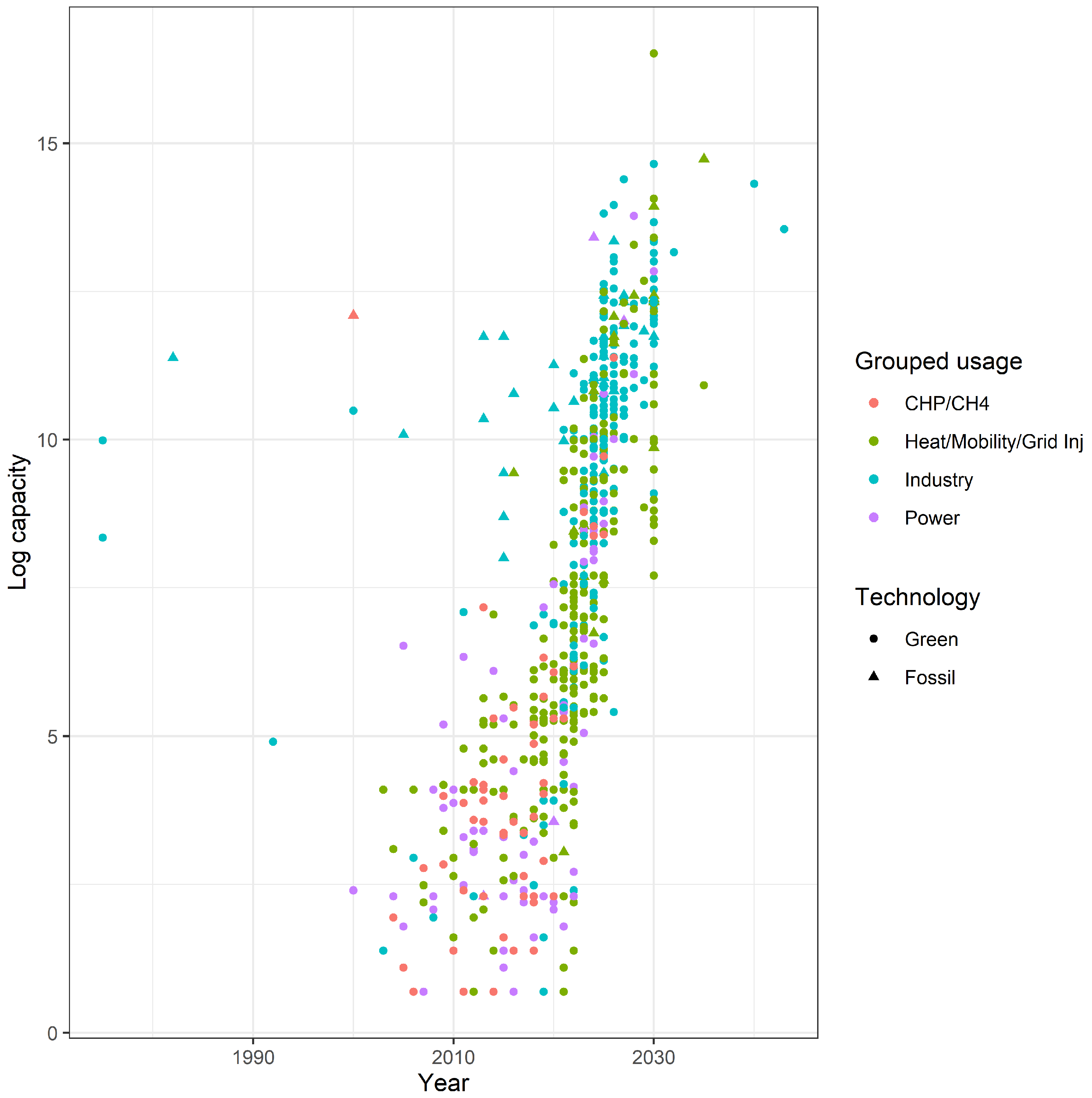
5. Trends in Capacity over Time and Relative to Technology and End-Use Sector

In this section, we examine the increase in capacity of low-carbon hydrogen plants over time while examining differences between technology and end-use sector. In Figure 5, we display all plants with an identified technology, end-use sector, and capacity in our dataset. Displaying the logarithm of the capacity against the year (or projected year) of construction, we see an approximate linear trend between the log of capacity and time, suggesting an exponential increase in capacity over time. We separate plants’ hydrogen technology into green and blue/fossil and separate them into end-use sectors. For graphical readability, we have chosen to separate sectors into the four clusters discussed in Section 3 that were determined in Figure 2. These are: the seven industrial applications, the three consumer/domestic sectors (domestic heat, grid injection, mobility), the CHP/CH4 outlier cluster, and the single outlier (power).
For robustness, we also repeated this plot with some slightly different groupings. For example, we separated CHP from the two CH4 uses, and we separated domestic heat from mobility/grid injection (as domestic heat is not quite as similar as the latter two in Figure 2). No substantial differences were observed in the log capacity vs. year scatter plot, so we proceed with the groupings from Figure 2 as they are.
To confirm this exponential fit, we implemented a series of linear regressions between the (log) capacity, time, as well as technology and usage. Linear regression is a commonly used and celebrated statistical model. This method seeks to model a response or target variable (in this case capacity or log capacity) as a linear function of other variables, including time. The most suitable linear coefficients are determined by a process called least squared estimation [85], where the line of best fit is defined by the property that the sum of square deviations from that line is minimised. Linear regression is perhaps the simplest of all statistical or machine learning models; however, it is by no means trivial. In its simplicity, it can provide greater interpretability than much more complex models, and sometimes perform just as well. That is our aim today. We remark that our purpose is not predictive (predicting future trends in hydrogen plants) but to describe trends observed in the data as of now (including planned plants for future construction). Our linear regression models take one of the following forms:
y i = β 0 + β 1 t i + j β j u s e 1 i j u s e + β t e c h 1 i t e c h ,
log ( y i ) = β 0 + β 1 t i + j β j u s e 1 i j u s e + β t e c h 1 i t e c h ,
where y i is the capacity, t i is the year for each plant, and we include dummy variables for end-use sectors and technology (green or fossil). With only two technologies, only one dummy variable is necessary; for the end-use sectors, we require one fewer dummy variable than the number of sectors. We run eight linear regressions across three choices—capacity or log capacity, all 14 end-use sectors, or the four grouped usages as in Figure 2 and Figure 5—and the inclusion of the technology variable or not. We record the adjusted R 2 , a measure of goodness of fit, for all eight regressions in Table 1.
The results confirm the main finding visible in Figure 5, a clearly superior fit exists when considering the log capacity model across all other choices. This strongly suggests a rather regular exponential growth in the capacity of plants over time, including when separating across usage sectors. That is, we have used goodness-of-fit measures to reveal that the increase in capacity over time is better represented as exponential than linear, and rather well represented as exponential in its own right. Viewing Figure 5 across the usage groups tells a promising story. With the exception of the industrial sectors, which saw a relatively early onset of high-capacity plants (though few in number), the other groups are growing at a commensurate rate, as can be seen by the relative collinearity of domestic heat/mobility/grid injection, CHP/CH4, and power. We can also see the welcome closing of the gap between green and blue/fossil hydrogen plants’ capacities.

6. Conclusions

This paper studies the capacity and end-use sectors of low-carbon hydrogen technologies over time, between green (zero-carbon) or blue/fossil (captured and stored carbon) technologies, and differences across the world. Combining the findings from investigating the distinct phenomena explored in this paper provides a unique, holistic overview regarding the state of low-carbon hydrogen projects globally. We are unaware of any similar work in the application field of low-carbon hydrogen.
In Section 3, we investigate the distributions of new hydrogen plants over time. Our results show a welcome growth in new and planned plants in recent years and the 2020’s, consistent across sectors. By analysing the discrepancy between temporal cumulative distribution functions, we reveal interesting structural similarity, including a strong cluster of industrial applications, where the number of plants is presently increasing significantly, and a smaller cluster of domestic applications. Some outlier end-use sectors are also revealed, particularly power, which has been much more consistent and uniform in its increase in new plants over time, heralding a more reliable and proven usage sector. Simply put, we classify end-use sectors as under uniform growth (power), concave-up growth (domestic applications), and explosive growth (industrial applications).
In Section 4, we study usage distributions of end-use sector across continental and technological groupings of hydrogen plants, both across the entire period of analysis and on a decade-by-decade basis. We reveal additional structural similarity, including the greatest diversity of usages among green power plants of the four most economically advanced continents, a welcome sign of the widespread utility and diverse applications of hydrogen energy. Interestingly, single key end-use sectors can almost entirely explain the broad-level cluster structure, such as ammonia across the entire period and the 2020–2029 decade, power in the 2000–2009 decade, and mobility and power in the 2010–2019 decade.
Finally, in Section 5, we demonstrate the changing relationship between green and blue hydrogen project capacity across a range of sectors (and the groupings determined by Section 3). We observe both graphically and analytically an exponential growth in the capacity of green hydrogen projects across all sectors, both grouped and ungrouped. This is an excellent sign for the future of this renewable fuel and suggests that investing in green hydrogen projects will likely provide returns in the coming years, regardless of end-use sector. Indeed, the diversity of the end-use applications, especially with exponentially increasing capacity of plants, means that the market for hydrogen technology is both growing and inherently diversified. This reflects well on the potential returns in governments and private entities investing in this technology, as well as less risk than a technology with more limited uses.
The future development of hydrogen plants must consider safety, profitability, and widespread utility of hydrogen production, all to further the key aim of decarbonisation, while blue hydrogen plants discussed in this manuscript attempt to sequester their carbon emissions, the use of oil, coal, or natural gas in the process carries a significant risk of harmful byproducts, and the capture of emissions is imperfect [86]. Thus, we hope to see growth in the number of green hydrogen plants across all end-use sectors, providing useful benefits to a diverse range of societal sectors, and associated increases in their capacity. Monitoring these trends may be crucial to the future of decarbonisation for many industries as diverse societies drive towards a sustainable existence.

Author Contributions

N.J. and M.M. contributed equally in every aspect of the paper. All authors have read and agreed to the published version of the manuscript.

Funding

This research received no external funding.

Data Availability Statement

The data analysed in this article are publicly available at [80]. A cached copy is available at https://github.com/MaxMenzies/HydrogenData (accessed on 26 November 2022).

Conflicts of Interest

The authors declare no conflict of interest.

Appendix A. Probability Distribution Distance

In this appendix, we give a technical explanation of why our distance (Equation (2)) can be interpreted as perhaps the most appropriate distance between two distributions on a discrete set. Let ( X , d ) be a metric space, μ , ν two probability measures on X, and q 1 a real number. The Wasserstein metric between distributions μ , ν is defined as
W q ( μ , ν ) = inf γ X × X d ( x , y ) q d γ 1 q ,
where the infimum is taken over all probability measures γ on X × X with marginal distributions μ and ν , respectively. From here, let q = 1 . By the Kantorovich–Rubinstein formula [87], there is an alternative formulation of Equation (A1) when X is compact (for example, finite):
W 1 ( μ , ν ) = sup F X F d μ X F d ν ,
where the supremum is taken over all 1-Lipschitz functions F : X R , meaning | F ( x , y ) | d ( x , y ) for all x , y .
Proposition A1.
Let ( X , d ) be a finite set with the discrete metric, with d ( x , y ) = 1 for x y and 0 otherwise. Let W 1 ( μ , ν ) be the L 1 -Wasserstein metric between two probability measures μ , ν on X, as expressed in Equation (A2). That is,
W 1 ( μ , ν ) = sup F X F d μ X F d ν .
Associate to μ and ν corresponding distribution functions or probability vectors f and g, respectively.
Then, the supremum written above is optimised by the following choice of F:
F ( x ) = 1 , f ( x ) g ( x ) , 0 , f ( x ) < g ( x ) .
Thus, W 1 ( f , g ) reduces to the same form of Equation (2), namely
W 1 ( f , g ) = 1 2 | | f g | | 1 .
Proof. 
Let F be an arbitrary 1-Lipschitz function on X with its discrete metric. Thus, F : X R and | F ( x ) F ( y ) | d ( x , y ) 1 for all x , y . We define M and m by M = sup x X F ( x ) and m = inf y X F ( y ) . By taking the supremum over elements x and the infimum over y, the Lipschitz condition implies that M m 1 . So
X F d μ X F d ν = x X F ( x ) ( f ( x ) g ( x ) )
x : f ( x ) g ( x ) M ( f ( x ) g ( x ) ) + x : f ( x ) < g ( x ) m ( f ( x ) g ( x ) )
x : f ( x ) g ( x ) ( m + 1 ) ( f ( x ) g ( x ) ) + x : f ( x ) < g ( x ) m ( f ( x ) g ( x ) )
= x : f ( x ) g ( x ) f ( x ) g ( x ) + x X m ( f ( x ) g ( x ) )
= x : f ( x ) g ( x ) f ( x ) g ( x ) ,
using the fact that x f ( x ) = x g ( x ) = 1 to eliminate the second summand of Equation (A6). Next, we set
P = x : f ( x ) g ( x ) f ( x ) g ( x ) ,
N = x : f ( x ) < g ( x ) g ( x ) f ( x ) .
So P N = x X f ( x ) g ( x ) = 0 , whereas P + N = x X | f ( x ) g ( x ) | = f g 1 . It follows P = N = 1 2 f g 1 , and X F d μ X F d ν P . Taking the supremum over F, we determine W 1 ( f , g ) P . Finally, let F be the function defined in the proposition Statement (A4). Then, X F d μ X F d ν coincides with P by definition. Thus, the supremal value W 1 ( f , g ) coincides exactly with P, and P = 1 2 f g 1 , as required. □

References

  1. Anandakugan, N.; U.S. Energy Information Administration. Coal Explained: Coal and the Environment. 2022. Available online: https://www.eia.gov/energyexplained/coal/coal-and-the-environment.php (accessed on 26 November 2022).
  2. Doenitz, W.; Schmidberger, R.; Steinheil, E.; Streicher, R. Hydrogen production by high temperature electrolysis of water vapour. Int. J. Hydrog. Energy 1980, 5, 55–63. [Google Scholar] [CrossRef]
  3. Wendt, H.; Plzak, V. Hydrogen production by water electrolysis / Wasserstoffproduktion durch Elektrolyse von Wasser. Kerntechnik 1991, 56, 22–28. [Google Scholar] [CrossRef]
  4. Khaselev, O. High-efficiency integrated multijunction photovoltaic/electrolysis systems for hydrogen production. Int. J. Hydrog. Energy 2001, 26, 127–132. [Google Scholar] [CrossRef]
  5. Ursua, A.; Gandia, L.M.; Sanchis, P. Hydrogen Production From Water Electrolysis: Current Status and Future Trends. Proc. IEEE 2012, 100, 410–426. [Google Scholar] [CrossRef]
  6. Chi, J.; Yu, H. Water electrolysis based on renewable energy for hydrogen production. Chin. J. Catal. 2018, 39, 390–394. [Google Scholar] [CrossRef]
  7. Zeng, K.; Zhang, D. Recent progress in alkaline water electrolysis for hydrogen production and applications. Prog. Energy Combust. Sci. 2010, 36, 307–326. [Google Scholar] [CrossRef]
  8. Barbir, F. PEM electrolysis for production of hydrogen from renewable energy sources. Sol. Energy 2005, 78, 661–669. [Google Scholar] [CrossRef]
  9. Grigoriev, S.; Porembsky, V.; Fateev, V. Pure hydrogen production by PEM electrolysis for hydrogen energy. Int. J. Hydrog. Energy 2006, 31, 171–175. [Google Scholar] [CrossRef]
  10. Bessarabov, D.G.; Wang, H.; Li, H.; Zhao, N. (Eds.) PEM Electrolysis for Hydrogen Production: Principles and Applications; CRC Press: Boca Raton, FL, USA, 2016. [Google Scholar]
  11. Guo, Y.; Li, G.; Zhou, J.; Liu, Y. Comparison between hydrogen production by alkaline water electrolysis and hydrogen production by PEM electrolysis. IOP Conf. Ser. Earth Environ. Sci. 2019, 371, 042022. [Google Scholar] [CrossRef]
  12. Yilmaz, C.; Kanoglu, M. Thermodynamic evaluation of geothermal energy powered hydrogen production by PEM water electrolysis. Energy 2014, 69, 592–602. [Google Scholar] [CrossRef]
  13. Rozendal, R.; Hamelers, H.; Euverink, G.; Metz, S.; Buisman, C. Principle and perspectives of hydrogen production through biocatalyzed electrolysis. Int. J. Hydrog. Energy 2006, 31, 1632–1640. [Google Scholar] [CrossRef]
  14. Call, D.; Logan, B.E. Hydrogen Production in a Single Chamber Microbial Electrolysis Cell Lacking a Membrane. Environ. Sci. Technol. 2008, 42, 3401–3406. [Google Scholar] [CrossRef] [PubMed]
  15. Rai, C.; Bhui, B.; V, P. Techno-economic analysis of e-waste based chemical looping reformer as hydrogen generator with co-generation of metals, electricity and syngas. Int. J. Hydrog. Energy 2022, 47, 11177–11189. [Google Scholar] [CrossRef]
  16. Wang, M.; Wang, Z.; Gong, X.; Guo, Z. The intensification technologies to water electrolysis for hydrogen production—A review. Renew. Sustain. Energy Rev. 2014, 29, 573–588. [Google Scholar] [CrossRef]
  17. Chakik, F.E.; Kaddami, M.; Mikou, M. Effect of operating parameters on hydrogen production by electrolysis of water. Int. J. Hydrog. Energy 2017, 42, 25550–25557. [Google Scholar] [CrossRef]
  18. Wu, L.; Zhou, Z.; Xiao, Y.; Xu, Z.; Li, X. Hydrogen evolution reaction activity and stability of sintered porous Ni-Cu-Ti-La2O3 cathodes in a wide pH range. Int. J. Hydrog. Energy 2022, 47, 11101–11115. [Google Scholar] [CrossRef]
  19. Ikeda, H.; Misumi, R.; Kojima, Y.; Haleem, A.A.; Kuroda, Y.; Mitsushima, S. Microscopic high-speed video observation of oxygen bubble generation behavior and effects of anode electrode shape on OER performance in alkaline water electrolysis. Int. J. Hydrog. Energy 2022, 47, 11116–11127. [Google Scholar] [CrossRef]
  20. Zhang, H.; Lin, G.; Chen, J. Evaluation and calculation on the efficiency of a water electrolysis system for hydrogen production. Int. J. Hydrog. Energy 2010, 35, 10851–10858. [Google Scholar] [CrossRef]
  21. Shit, S.; Bolar, S.; Kolya, H.; Kang, C.W.; Murmu, N.C.; Kuila, T. Assisting the formation of S-doped FeMoO4 in lieu of an iron oxide/molybdenum sulfide heterostructure: A unique approach towards attaining excellent electrocatalytic water splitting activity. Int. J. Hydrog. Energy 2022, 47, 11128–11142. [Google Scholar] [CrossRef]
  22. Tong, L.; Liu, Y.; Song, C.; Zhang, Y.; Latthe, S.S.; Liu, S.; Xing, R. (Fe, Ni)S2@MoS2/NiS2 hollow heterostructure nanocubes for high-performance alkaline water electrolysis. Int. J. Hydrog. Energy 2022, 47, 11143–11152. [Google Scholar] [CrossRef]
  23. Liang, S.; Sui, G.; Li, J.; Guo, D.; Luo, Z.; Xu, R.; Yao, H.; Wang, C.; Chen, S. ZIF-L-derived porous C-doped ZnO/CdS graded nanorods with Z-scheme heterojunctions for enhanced photocatalytic hydrogen evolution. Int. J. Hydrog. Energy 2022, 47, 11190–11202. [Google Scholar] [CrossRef]
  24. Khasanah, R.A.N.; Lin, H.C.; Ho, H.Y.; Peng, Y.P.; Hsiao, H.L.; Wang, C.R.; Chien, F.S.S. Photoelectrocatalytic hydrolysis of ammonia borane by electrochemical deposited cuprous oxide on titanium dioxide nanotube arrays. Int. J. Hydrog. Energy 2022, 47, 11203–11210. [Google Scholar] [CrossRef]
  25. Liu, Y.; Shi, X.; Liu, X.; Li, X. Facile synthesis of C-Ta4+ co-doped NaTaO3 and rGO nanocomposites with enhanced visible light photocatalytic performance. Int. J. Hydrog. Energy 2022, 47, 11211–11223. [Google Scholar] [CrossRef]
  26. Ulate-Kolitsky, E.; Tougas, B.; Huot, J. First Hydrogenation of TiFe with Addition of 20 wt.% Ti. Hydrogen 2022, 3, 379–388. [Google Scholar] [CrossRef]
  27. He, J.; Han, X.; Xiang, H.; Ran, R.; Wang, W.; Zhou, W.; Shao, Z. Aluminum Cation Doping in Ruddlesden-Popper Sr2TiO4 Enables High-Performance Photocatalytic Hydrogen Evolution. Hydrogen 2022, 3, 501–511. [Google Scholar] [CrossRef]
  28. Sołowski, G.; Shalaby, M.; Özdemir, F.A. Plastic and Waste Tire Pyrolysis Focused on Hydrogen Production—A Review. Hydrogen 2022, 3, 531–549. [Google Scholar] [CrossRef]
  29. Shelepova, E.V.; Maksimova, T.A.; Bauman, Y.I.; Mishakov, I.V.; Vedyagin, A.A. Experimental and Simulation Study on Coproduction of Hydrogen and Carbon Nanomaterials by Catalytic Decomposition of Methane-Hydrogen Mixtures. Hydrogen 2022, 3, 450–462. [Google Scholar] [CrossRef]
  30. Vedyagin, A.A.; Mishakov, I.V.; Korneev, D.V.; Bauman, Y.I.; Nalivaiko, A.Y.; Gromov, A.A. Selected Aspects of Hydrogen Production via Catalytic Decomposition of Hydrocarbons. Hydrogen 2021, 2, 122–133. [Google Scholar] [CrossRef]
  31. Lys, A.; Fadonougbo, J.O.; Faisal, M.; Suh, J.Y.; Lee, Y.S.; Shim, J.H.; Park, J.; Cho, Y.W. Enhancing the Hydrogen Storage Properties of AxBy Intermetallic Compounds by Partial Substitution: A Short Review. Hydrogen 2020, 1, 38–63. [Google Scholar] [CrossRef]
  32. Heinemann, N.; Wilkinson, M.; Adie, K.; Edlmann, K.; Thaysen, E.M.; Hassanpouryouzband, A.; Haszeldine, R.S. Cushion Gas in Hydrogen Storage—A Costly CAPEX or a Valuable Resource for Energy Crises? Hydrogen 2022, 3, 550–563. [Google Scholar] [CrossRef]
  33. Pistidda, C. Solid-State Hydrogen Storage for a Decarbonized Society. Hydrogen 2021, 2, 428–443. [Google Scholar] [CrossRef]
  34. Ekhtiari, A.; Flynn, D.; Syron, E. Green Hydrogen Blends with Natural Gas and Its Impact on the Gas Network. Hydrogen 2022, 3, 402–417. [Google Scholar] [CrossRef]
  35. Lattin, W.; Utgikar, V. Transition to hydrogen economy in the United States: A 2006 status report. Int. J. Hydrog. Energy 2007, 32, 3230–3237. [Google Scholar] [CrossRef]
  36. Park, S. The country-dependent shaping of ‘hydrogen niche’ formation: A comparative case study of the UK and South Korea from the innovation system perspective. Int. J. Hydrog. Energy 2013, 38, 6557–6568. [Google Scholar] [CrossRef]
  37. Yuan, K.; Lin, W. Hydrogen in China: Policy, program and progress. Int. J. Hydrog. Energy 2010, 35, 3110–3113. [Google Scholar] [CrossRef]
  38. Collera, A.A.; Agaton, C.B. Opportunities for production and utilization of green hydrogen in the Philippines. Int. J. Energy Econ. Policy 2021, 11, 37–41. [Google Scholar] [CrossRef]
  39. Ramirez-Salgado, J.; Estrada-Martinez, A. Roadmap towards a sustainable hydrogen economy in Mexico. J. Power Sources 2004, 129, 255–263. [Google Scholar] [CrossRef]
  40. Touili, S.; Alami Merrouni, A.; Azouzoute, A.; El Hassouani, Y.; Amrani, A.i. A technical and economical assessment of hydrogen production potential from solar energy in Morocco. Int. J. Hydrog. Energy 2018, 43, 22777–22796. [Google Scholar] [CrossRef]
  41. Apak, S.; Atay, E.; Tuncer, G. Renewable hydrogen energy regulations, codes and standards: Challenges faced by an EU candidate country. Int. J. Hydrog. Energy 2012, 37, 5481–5497. [Google Scholar] [CrossRef]
  42. James, N.; Menzies, M. Spatio-temporal trends in the propagation and capacity of low-carbon hydrogen projects. Int. J. Hydrog. Energy 2022, 47, 16775–16784. [Google Scholar] [CrossRef]
  43. Bridgeland, R.; Chapman, A.; McLellan, B.; Sofronis, P.; Fujii, Y. Challenges toward achieving a successful hydrogen economy in the US: Potential end-use and infrastructure analysis to the year 2100. Clean. Prod. Lett. 2022, 3, 100012. [Google Scholar] [CrossRef]
  44. Saeedmanesh, A.; Kinnon, M.A.M.; Brouwer, J. Hydrogen is essential for sustainability. Curr. Opin. Electrochem. 2018, 12, 166–181. [Google Scholar] [CrossRef]
  45. Dawood, F.; Anda, M.; Shafiullah, G. Hydrogen production for energy: An overview. Int. J. Hydrog. Energy 2020, 45, 3847–3869. [Google Scholar] [CrossRef]
  46. Pleshivtseva, Y.; Derevyanov, M.; Pimenov, A.; Rapoport, A. Comprehensive review of low carbon hydrogen projects towards the decarbonization pathway. Int. J. Hydrog. Energy 2023, 48, 3703–3724. [Google Scholar] [CrossRef]
  47. Manchein, C.; Brugnago, E.L.; da Silva, R.M.; Mendes, C.F.O.; Beims, M.W. Strong correlations between power-law growth of COVID-19 in four continents and the inefficiency of soft quarantine strategies. Chaos Interdiscip. J. Nonlinear Sci. 2020, 30, 041102. [Google Scholar] [CrossRef] [PubMed]
  48. James, N.; Menzies, M.; Bondell, H. Comparing the dynamics of COVID-19 infection and mortality in the United States, India, and Brazil. Phys. D Nonlinear Phenom. 2022, 432, 133158. [Google Scholar] [CrossRef]
  49. Li, H.J.; Xu, W.; Song, S.; Wang, W.X.; Perc, M. The dynamics of epidemic spreading on signed networks. Chaos Solitons Fractals 2021, 151, 111294. [Google Scholar] [CrossRef]
  50. Blasius, B. Power-law distribution in the number of confirmed COVID-19 cases. Chaos Interdiscip. J. Nonlinear Sci. 2020, 30, 093123. [Google Scholar] [CrossRef]
  51. James, N.; Menzies, M. Estimating a continuously varying offset between multivariate time series with application to COVID-19 in the United States. Eur. Phys. J. Spec. Top. 2022, 231, 3419–3426. [Google Scholar] [CrossRef]
  52. Perc, M.; Miksić, N.G.; Slavinec, M.; Stožer, A. Forecasting COVID-19. Front. Phys. 2020, 8, 127. [Google Scholar] [CrossRef] [Green Version]
  53. Machado, J.A.T.; Lopes, A.M. Rare and extreme events: The case of COVID-19 pandemic. Nonlinear Dyn. 2020, 100, 2953–2972. [Google Scholar] [CrossRef] [PubMed]
  54. James, N.; Menzies, M. Global and regional changes in carbon dioxide emissions: 1970–2019. Phys. A Stat. Mech. Appl. 2022, 608, 128302. [Google Scholar] [CrossRef]
  55. Khan, M.K.; Khan, M.I.; Rehan, M. The relationship between energy consumption, economic growth and carbon dioxide emissions in Pakistan. Financ. Innov. 2020, 6, 1. [Google Scholar] [CrossRef] [Green Version]
  56. James, N.; Menzies, M. Equivalence relations and Lp distances between time series with application to the Black Summer Australian bushfires. Phys. D Nonlinear Phenom. 2023, 448, 133693. [Google Scholar] [CrossRef]
  57. Drożdż, S.; Kwapień, J.; Oświęcimka, P. Complexity in Economic and Social Systems. Entropy 2021, 23, 133. [Google Scholar] [CrossRef] [PubMed]
  58. James, N.; Menzies, M.; Gottwald, G.A. On financial market correlation structures and diversification benefits across and within equity sectors. Phys. A Stat. Mech. Appl. 2022, 604, 127682. [Google Scholar] [CrossRef]
  59. Liu, Y.; Cizeau, P.; Meyer, M.; Peng, C.K.; Stanley, H.E. Correlations in economic time series. Phys. A Stat. Mech. Appl. 1997, 245, 437–440. [Google Scholar] [CrossRef] [Green Version]
  60. Basalto, N.; Bellotti, R.; Carlo, F.D.; Facchi, P.; Pantaleo, E.; Pascazio, S. Hausdorff clustering of financial time series. Phys. A Stat. Mech. Appl. 2007, 379, 635–644. [Google Scholar] [CrossRef] [Green Version]
  61. Wątorek, M.; Kwapień, J.; Drożdż, S. Financial Return Distributions: Past, Present, and COVID-19. Entropy 2021, 23, 884. [Google Scholar] [CrossRef]
  62. Prakash, A.; James, N.; Menzies, M.; Francis, G. Structural Clustering of Volatility Regimes for Dynamic Trading Strategies. Appl. Math. Financ. 2021, 28, 236–274. [Google Scholar] [CrossRef]
  63. Drożdż, S.; Grümmer, F.; Ruf, F.; Speth, J. Towards identifying the world stock market cross-correlations: DAX versus Dow Jones. Phys. A Stat. Mech. Appl. 2001, 294, 226–234. [Google Scholar] [CrossRef] [Green Version]
  64. James, N.; Menzies, M.; Chin, K. Economic state classification and portfolio optimisation with application to stagflationary environments. Chaos Solitons Fractals 2022, 164, 112664. [Google Scholar] [CrossRef]
  65. Gębarowski, R.; Oświęcimka, P.; Wątorek, M.; Drożdż, S. Detecting correlations and triangular arbitrage opportunities in the Forex by means of multifractal detrended cross-correlations analysis. Nonlinear Dyn. 2019, 98, 2349–2364. [Google Scholar] [CrossRef] [Green Version]
  66. James, N.; Menzies, M. A new measure between sets of probability distributions with applications to erratic financial behavior. J. Stat. Mech. Theory Exp. 2021, 2021, 123404. [Google Scholar] [CrossRef]
  67. Sigaki, H.Y.D.; Perc, M.; Ribeiro, H.V. Clustering patterns in efficiency and the coming-of-age of the cryptocurrency market. Sci. Rep. 2019, 9, 1440. [Google Scholar] [CrossRef] [PubMed] [Green Version]
  68. Drożdż, S.; Kwapień, J.; Oświęcimka, P.; Stanisz, T.; Wątorek, M. Complexity in Economic and Social Systems: Cryptocurrency Market at around COVID-19. Entropy 2020, 22, 1043. [Google Scholar] [CrossRef]
  69. James, N.; Menzies, M. Collective correlations, dynamics, and behavioural inconsistencies of the cryptocurrency market over time. Nonlinear Dyn. 2022, 107, 4001–4017. [Google Scholar] [CrossRef]
  70. Drożdż, S.; Minati, L.; Oświęcimka, P.; Stanuszek, M.; Wątorek, M. Competition of noise and collectivity in global cryptocurrency trading: Route to a self-contained market. Chaos: Interdiscip. J. Nonlinear Sci. 2020, 30, 023122. [Google Scholar] [CrossRef] [PubMed] [Green Version]
  71. Wątorek, M.; Drożdż, S.; Kwapień, J.; Minati, L.; Oświęcimka, P.; Stanuszek, M. Multiscale characteristics of the emerging global cryptocurrency market. Phys. Rep. 2021, 901, 1–82. [Google Scholar] [CrossRef]
  72. James, N.; Menzies, M. Dual-domain analysis of gun violence incidents in the United States. Chaos Interdiscip. J. Nonlinear Sci. 2022, 32, 111101. [Google Scholar] [CrossRef]
  73. Perc, M.; Donnay, K.; Helbing, D. Understanding Recurrent Crime as System-Immanent Collective Behavior. PLoS ONE 2013, 8, e76063. [Google Scholar] [CrossRef] [Green Version]
  74. James, N.; Menzies, M.; Chok, J.; Milner, A.; Milner, C. Geometric persistence and distributional trends in worldwide terrorism. Chaos Solitons Fractals 2023, 169, 113277. [Google Scholar] [CrossRef]
  75. Ribeiro, H.V.; Mukherjee, S.; Zeng, X.H.T. Anomalous diffusion and long-range correlations in the score evolution of the game of cricket. Phys. Rev. E 2012, 86, 022102. [Google Scholar] [CrossRef] [Green Version]
  76. James, N.; Menzies, M. Optimally adaptive Bayesian spectral density estimation for stationary and nonstationary processes. Stat. Comput. 2022, 32, 45. [Google Scholar] [CrossRef]
  77. Merritt, S.; Clauset, A. Scoring dynamics across professional team sports: Tempo, balance and predictability. EPJ Data Sci. 2014, 3, 4. [Google Scholar] [CrossRef] [Green Version]
  78. James, N.; Menzies, M.; Bondell, H. In search of peak human athletic potential: A mathematical investigation. Chaos Interdiscip. J. Nonlinear Sci. 2022, 32, 023110. [Google Scholar] [CrossRef]
  79. Clauset, A.; Kogan, M.; Redner, S. Safe leads and lead changes in competitive team sports. Phys. Rev. E 2015, 91, 062815. [Google Scholar] [CrossRef] [Green Version]
  80. International Energy Agency. Hydrogen Projects Database. 2022. Available online: https://www.iea.org/data-and-statistics/data-product/hydrogen-projects-database (accessed on 1 November 2022).
  81. Ward, J.H. Hierarchical Grouping to Optimize an Objective Function. J. Am. Stat. Assoc. 1963, 58, 236–244. [Google Scholar] [CrossRef]
  82. Szekely, G.J.; Rizzo, M.L. Hierarchical Clustering via Joint Between-Within Distances: Extending Ward’s Minimum Variance Method. J. Classif. 2005, 22, 151–183. [Google Scholar] [CrossRef]
  83. Müllner, D. Fastcluster: Fast Hierarchical, Agglomerative Clustering Routines forRandPython. J. Stat. Softw. 2013, 53, 1–18. [Google Scholar] [CrossRef] [Green Version]
  84. James, N.; Menzies, M.; Bondell, H. Understanding spatial propagation using metric geometry with application to the spread of COVID-19 in the United States. Europhys. Lett. 2021, 135, 48004. [Google Scholar] [CrossRef]
  85. James, G.; Witten, D.; Hastie, T.; Tibshirani, R. An Introduction to Statistical Learning; Springer: New York, NY, USA, 2013. [Google Scholar] [CrossRef]
  86. Intergovernmental Panel on Climate Change. Carbon Dioxide Capture and Storage. 2005. Available online: https://www.ipcc.ch/site/assets/uploads/2018/03/srccs_wholereport-1.pdf (accessed on 26 November 2022).
  87. Kantorovich, L.V.; Rubinstein, G. On a space of completely additive functions. Vestn. Leningr. Univ. 1958, 13, 52–59. [Google Scholar]
Figure 1. Cumulative distribution functions F S for eight sectors S, (a) refining (b) ammonia (c) synfuels (d) methanol (e) mobility (f) domestic heat (g) CHP (h) power. Sectors are described in Section 2. The greatest collective similarity is observed between industrial applications, with an explosion of planned plants in the 2020’s. Power serves as an anomaly with its highly uniform trend of new plants.
Hydrogen 04 00012 g001
Figure 2. Hierarchical clustering on cumulative distribution functions F S (relative to time) for all 14 end-use sectors S in our database. A strong cluster of similarity is observed for the seven industrial uses, ranging from biofuels to ammonia. A secondary cluster of more ‘consumer uses’ is revealed from grid injection to domestic heat, whereas power is observed as an outlier due to its highly uniform nature.
Hydrogen 04 00012 g002
Figure 3. Distribution dendrograms between continental/technological groups G, produced by hierarchical clustering on the distance (2) for (a) the entire period of analysis (b) 2000—2009 (c) 2010–2019 (d) 2020–2029 (e) 2030–2039. There are only 12 groups G as there are no fossil plants in Africa or Latin America.
Hydrogen 04 00012 g003
Figure 4. Stacked bar plots showing distribution of end-use sectors for (a) the entire period of analysis (b) 2000–2009 (c) 2010–2019 (d) 2020–2029 (e) 2030–2039. There are only 12 groups G as there are no fossil plants in Africa or Latin America. Empty bars indicate no plants in that group over that period.
Hydrogen 04 00012 g004
Figure 5. Log capacity vs. year of construction for all plants in our dataset with available data. We classify plants by both their technology as well as their usage, using the clusters of end-use sectors from Section 3 Figure 2. We can see the early dominance of blue plants (with a few early exceptions) by several orders of magnitude, but this is closing with time.
Hydrogen 04 00012 g005
Table 1. Adjusted R 2 , a measure of goodness of fit for eight different linear regression models between (log) capacity, grouped or ungrouped sectors, and technology. A far better fit is observed for the exponential models.
Adjusted R 2 No Separation by TechStratified by Tech
Grouped SectorsAll SectorsGrouped SectorsAll Sectors
Capacity0.02550.02040.02730.0226
Log capacity0.5690.5870.6070.622
Disclaimer/Publisher’s Note: The statements, opinions and data contained in all publications are solely those of the individual author(s) and contributor(s) and not of MDPI and/or the editor(s). MDPI and/or the editor(s) disclaim responsibility for any injury to people or property resulting from any ideas, methods, instructions or products referred to in the content.

