
Potential Coffee Distribution in a Central-Western Region of Mexico
by
 ,
,
Armando Avalos Jiménez
* ,
,
Susana María Lorena Marceleño Flores
,
Oyolsi Nájera González
and
Fernando Flores Vilchez
Secretaría de Investigación y Posgrado, Universidad Autónoma de Nayarit, Ciudad de la Cultura s/n, Col. Centro, Tepic C.P. 63000, Mexico
*
Author to whom correspondence should be addressed.
Ecologies 2023, 4(2), 269-287; https://doi.org/10.3390/ecologies4020018
Submission received: 26 January 2023
/
Revised: 21 March 2023
/
Accepted: 24 March 2023
/
Published: 3 April 2023
Abstract
:Currently, there is a world coffee production crisis which has been attributed, among other factors, to the COVID-19 pandemic that affected the development of productive agricultural activities. In this scenario, Mexico is in a declining situation by showing a reduction in coffee production areas in recent years. Therefore, it is necessary to promote actions that contribute to the recovery of the resource, particularly in the states with agricultural potential. In the present work, the potentially suitable areas for coffee cultivation are identified through the application of tools that allow for characterizing the biophysical conditions that define the current spatial distribution and, from the analysis of these characteristics, generate a Potential Distribution Model (PDM) of the suitable zones for coffee production. The methodology was developed through the application of the Maximum Entropy (MaxEnt) algorithm, starting with the collection and preparation of coffee presence records, followed by a correlation analysis and identification of significant variables, the subsequent execution of the model in various configurations to observe the contribution of each variable through a jackknife test, and finally validation of the model with a random sample selection of 30%, to achieve an AUC of 0.98 and TSS of 0.96. The present model was able to identify and quantify the environmentally suitable zones for coffee production, highlighting the regions with ideal potential for the specie. These results are intended to serve as a basis for the generation of planning strategies aimed at managing, improving, and increasing coffee production areas, as well as being used to establish biological corridors to promote biodiversity, conservation, and alternative economic activities such as tourism and furthermore for future work on the analysis of production scenarios and impacts of climate change. It is concluded that 30% of Nayarit’s territory has ideal conditions for coffee cultivation, especially the region delimited by the municipalities of Tepic and Xalisco, the eastern zone of Compostela, and the southwest of San Blas, which should be considered as a Priority Conservation Area (APC) for coffee cultivation in the state.
1. Introduction
Coffee (Coffea arabica L.) is one of the main consumer products marketed worldwide due to its high energy value associated with caffeine. This last component is classified as a stimulant of the central nervous system that produces a temporary effect of sensory activation in small doses that makes it preferred by the population, to the extent that currently there is a world average consumption of 1.8 kg of coffee per capita [1]. It is the second-most traded commodity after oil, fluctuating on the main stock exchanges such as the New York Stock Exchange [2] and being of great economic, sociocultural, and environmental importance for most producing countries [3].
Just a couple of decades ago, and particularly since 2008, coffee production worldwide maintained an upward trend, on par with international consumption which was also at its maximum levels, increasing at an average annual rate of 2.80% [4]. By 2018, production reached its historical maximum in the last 20 years with a production of 10. 5 million tons of coffee, with Brazil being the main producer with more than 37% of world production, followed by Vietnam with a little more than 17% and Colombia with 8%; by this time, Mexico occupied the eighth place in world production with 2.4% according to data from the International Coffee Organization (ICO) [1].
The current situation of world production can be inferred from the most recent data of the ICO, which, for the year 2020, recorded a production of 9.9 million tons of coffee in the world, where only Brazil, Vietnam, Colombia, and Indonesia contributed 70% of total production. Since then, Brazil has stood out as the largest producer and exporter of coffee, but, in recent years (with respect to 2018), has reduced its production, reaching 33% of production. In second place is Vietnam [5], with 17% of world production, almost the same amount that is exported. In this same tenor is Mexico where, although its contribution is minimal compared to the main producers, it is of great relevance for the country, because, although it occupies the ninth place, it contributes a production of 2. 3%, corresponding to almost 240 thousand tons of coffee; and it is in the eleventh place in exports, with an amount of 177 thousand tons, equivalent to more than 2% of world exports [1].
Coffee production is one of the main agricultural activities in Mexico [2], considered of great economic, sociocultural, and environmental importance [3,6,7], integrating into different production chains for the creation of employment and contribution to the economy with the generation of foreign exchange [8] that allows the subsistence of many small producers. In addition to a high economic value, coffee production has an important contribution in environmental matters as it is a species that, when developed in shaded systems, maintains an almost permanent vegetation cover on the soil with its cultivation [9], which provides important ecosystem services by reducing soil erosion problems, contributing to the conservation of biological diversity [10,11] and serving as a refuge for wildlife [12,13] by propitiating water infiltration for groundwater recovery and soil conservation [14,15], as well as favoring carbon sequestration [16,17] and oxygen production, among other effects.
In spite of the positive aspects that these data may represent, it has recently been highlighted that there is a coffee production crisis in the world that has been mainly attributed to the COVID-19 pandemic that affected the development of most of the agricultural productive activities [18,19,20]. In Mexico, the production is currently in a situation of decadence due to the reduction in the amount of coffee production areas observed in recent years. In view of this scenario, it is necessary to promote actions that contribute to the recovery of the resource, it being essential to identify the zones that are adequate (suitable habitats) and that provide the necessary environmental conditions and characteristics for coffee production, in order to subsequently establish planning strategies focused on managing, improving, and increasing productivity.
The combination of all these economic, social, and environmental benefits generated by coffee cultivation and the downward trend in its production makes it necessary to contribute to the recovery of the resource, and, therefore, it is essential to have spatial information that reflects the areas that are potentially suitable in the central–western region of Mexico for coffee production and whose zoning characteristics should be assessed before they are lost. In this sense, the Species Distribution Models (SDMs) have represented a good approximation to find the regions of suitable habitat for the survival of a species, contemplating the environmental conditions in which they subsist [21].
SDMs base their principles on the concept of the Ecological Niche (EN), first introduced by Evelyn Hutchinson in 1957 as the set of biotic and abiotic conditions with which the species is related, allowing its existence in a given region [22], involving all the resources present for its development. In this context, ecological niche models and SDMs have similarities: on the one hand, the former relate environmental components and presence, presence–absence, and/or abundance data [23], while SDMs relate field observations with predictive environmental variables [24], based on a statistical response [21]. These have been widely used in the scientific community due to their efficiency in predicting the geographic distribution and exploring the preferred habitat of species [25], so a large number of them have been developed; among the most-used are statistical models: generalized linear models (GLM) and generalized additive models (GAM); heuristic models such as climate envelope (BIOCLIM); or others based on artificial intelligence techniques [26] and genetic algorithms for rule prediction (GARP) [27], as well as the MaxEnt model. The latter has gained popularity for being a machine learning method that has given better results and efficiency in model execution [28], offering advantages over the others by requiring only presence data (known distribution records) and layers of information on the environmental conditions of the area of influence of the known sites, with the objective of predicting the suitability of the environment for the specie based on their ecological niche [21].
MaxEnt is an algorithm used to estimate the probability of species distribution through the principle of MaxEnt, which was developed by [29], and is based on statistical procedures from real observational data on the presence or abundance of species, which it uses to infer potentially suitability according to their environmental characteristics, thus representing the suitability of a space for the presence of a species according to the variables used. This suitability is given by the mathematical relationship between the actual known distribution and the set of independent variables used as indicators. The model can generate response curves for each of the variables and estimate the importance or contribution of each of them in the distribution, as well as evaluating the effectiveness of the model.
The use of the MaxEnt model has been widely used in the scientific literature for a variety of applications, including: for determine the potential distribution of species [30], of both flora and fauna, to identify variables that determine suitable areas for species survival and conservation in predicting spatial patterns of biodiversity [31,32,33,34,35,36], in scenario analyses in the face of climate change [37,38,39,40] and prediction of its impact on species distribution [31,32,33,34,35,36,37,38,39,40,41,42,43,44,45,46], to determining the distribution of terrestrial reptiles [47], and in ecological niche studies [48], as well as to determine the potential distribution of pest or invasive species, as in [49,50,51]. The algorithm was also used by [52] to predict suitable habitat for the endangered tree Canacomyrica montícola and in Colombia for the species Pleurozia paradoxa [53], among many others.
In Mexico, these models have shown their capacity to be used to evaluate the distribution risk of diseases such as dengue [54]; to establish conservation proposals under climate change scenarios [55]; to predict the potential distribution of species such as the jaguar, the Mesoamerican tortoise, and species of forest interest of the genus Pinus [56,57,58]; for modeling the ecological niche of pine (Pinaceae) [23,55]; for modeling cyanobacteria and phytoplankton distribution [59,60]; and for modeling the distribution of plants such as Cuphea aequipetala Cav. (Lythraceae) [61], Cedro (Cedrela salvadorensis) [62], and avocado (Persea Mill) [63], among others.
Therefore, the objective of this work was to model the potential distribution of coffee by using the MaxEnt algorithm to characterize the biophysical conditions of the current distribution of coffee production and determine the potentially suitable areas. The methodology was developed from the collection and preparation of coffee presence data to subsequently running the model in different configurations to observe the contribution of each of the variables through the jackknife test. Consecutively, the necessary modifications were made to obtain the best fit of the model. Finally, it was validated with random selection of 30% of the coffee records of the sample to obtain the AUC (Area Under the Curve) and TSS (True Skill Statistics) with the best fit values.
2. Materials and Methods
2.1. Study Area
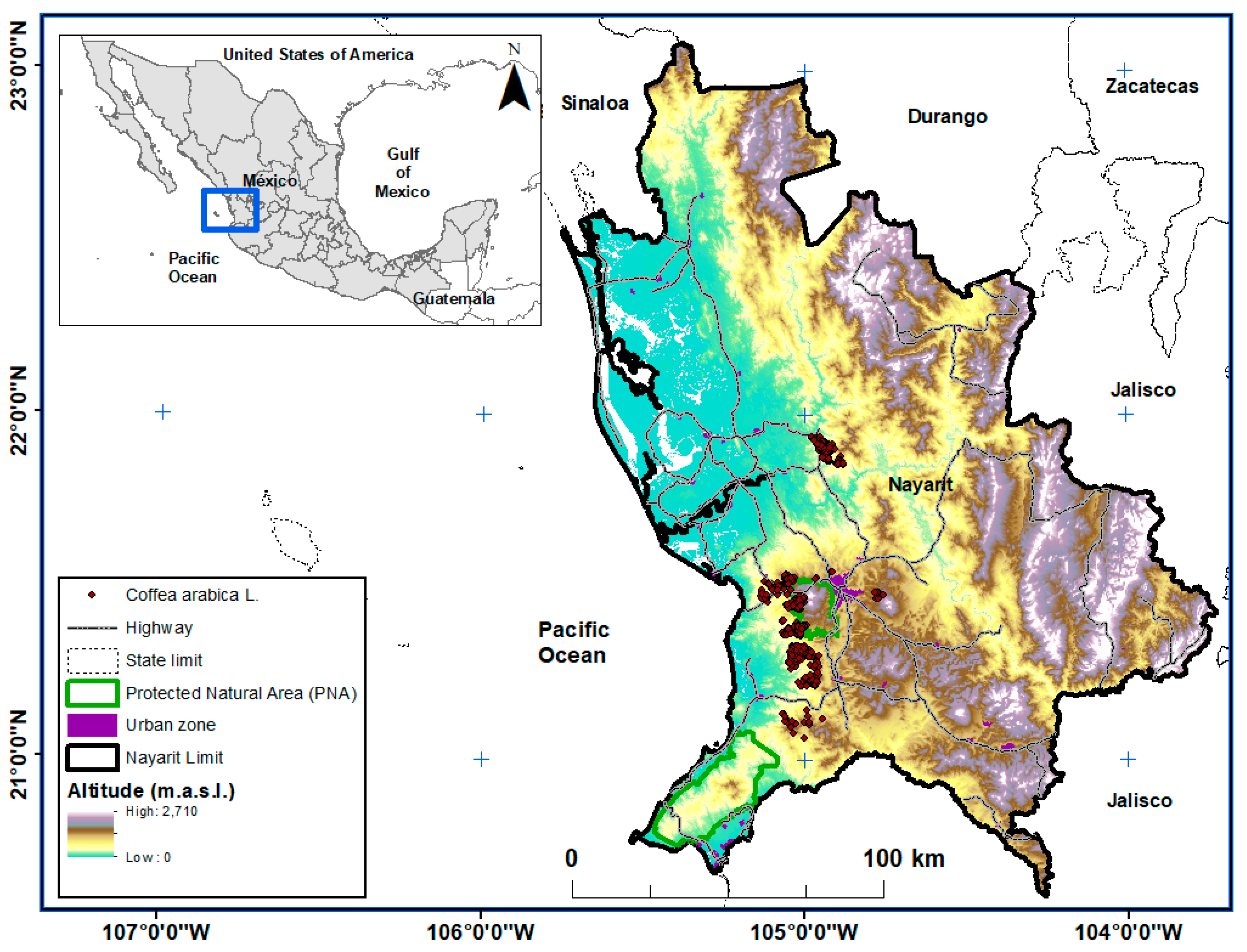
The study area was focused on the state of Nayarit located in the central western region of the United Mexican States (Mexico), bordering the states of Sinaloa and Durango to the north and Jalisco to the south-southeast, and also bordering the Pacific Ocean to the west as shown in Figure 1. The entity is divided into 20 municipalities with a land area of 27,888 km2 and a population of 1,235,456 inhabitants [64].
The study area focused on the central western region and particularly on the state of Nayarit from where the data were obtained, which is in the United Mexican States (Mexico) and borders the states of Sinaloa and Durango to the north and Jalisco to the south-southeast, also bordering the Pacific Ocean to the west as shown in Figure 1. The entity is divided into 20 Municipalities with a territorial extension of 27,888 km2 and a population of 1,235,456 people [64].
The study area is characterized in biophysical terms by being located between 104° and 106° north latitude and 21° and 23° west longitude, in an altitudinal range that goes from 0 to 2710 m above sea level (m.a.s.l.). It is among the states with the highest precipitation at the national level, with an annual average of 1200 mm, and has a warm sub-humid climate with summer rains. These and other factors together create a mosaic of landscapes that are ideal for a large number of species of flora and fauna, including coffee.
According to data obtained for the year 2020, the main coffee producers in Mexico were Veracruz, Chiapas, and Jalisco with almost 45% of the total planted area in the country. In 2020, coffee production in Mexico reached a planted area of almost ninety thousand km2 [65]. Currently, Nayarit is in a declining situation in coffee production, due to the reduction of planted area that has been occurring in recent years, according to records of the Ministry of Agriculture and Rural Development (SAGARPA). In 2012, there was a planted area of 162.46 km2, but this situation worsened by the year 2020, with only 33 square kilometers for the entire state, representing a reduction of almost 80% in a period of 8 years. If this trend continues, by 2030 there will only be 6 km2.
2.2. Presence Records Data
The starting point was the database of coffee presence records obtained through field visits, through interviews with producers, and with reference to the database provided by SAGARPA composed of 1658 records with three varieties of coffee of the Coffea arabica L. species: Typica (1604 records), Caturra (44 records), and Mundo Novo (10 records). Each record indicates the coordinate of the centroid of a polygon of land where coffee was observed.
2.3. Environmental Data
On the other hand, a set of 19 climatic variables were obtained from the WorldClim global meteorological and climatic database of high spatial resolution, which were downloaded from the web page (https://www.worldclim.org/, accessed on 20 November 2022), as well as the construction of seven other environmental variables obtained in a local representation and which are determinants for coffee production, finally resulting in a set of 26 variables described in Table 1.
2.4. Methodology
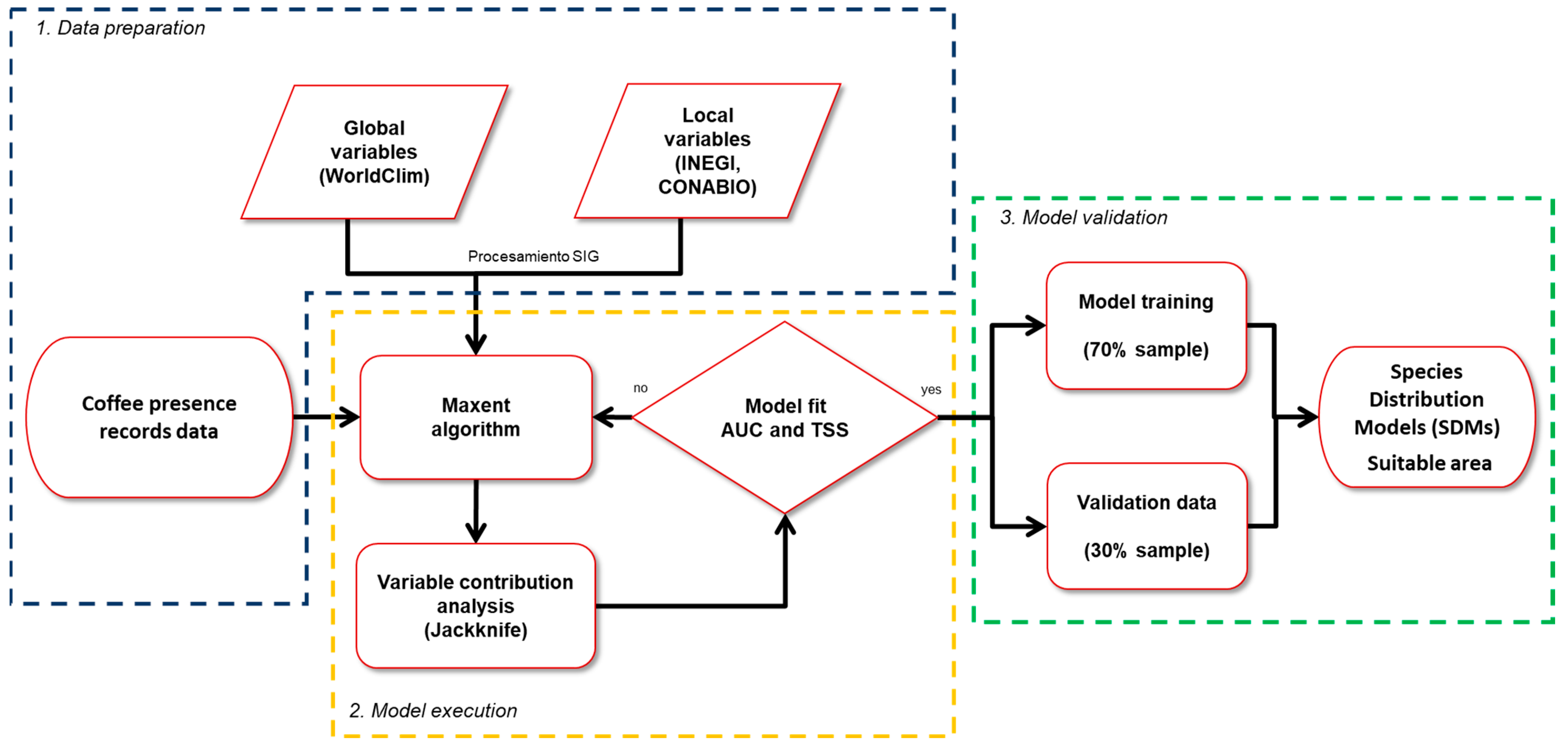
The methodology was developed in three stages; the first consisted of the collection of records of the presence of coffee species and the preparation of the data for the execution of the ecological niche model through the MaxEnt algorithm; the model was then run in different configurations (variation of model parameters) to analyze the contribution of each of the variables through the jackknife test and the necessary modifications were made to obtain the best fit of the model; finally, it was validated with the random selection of 30% of the species sample to obtain the AUC and TSS with the best fit values. This whole process is described in Figure 2.
2.4.1. Data Preparation
The species distribution model is based on the analysis of data records of occurrence or presence of species. For this, data on the presence of coffee with georeferenced coordinates in UTM were obtained and represented through geographic information systems for a first observation of its spatial distribution. On the other hand, variables were obtained from the WorldClim database in GRID format and others were built from the elevation model for the study area, land cover, and land use.
All the variables were processed through ArcGIS 10.3; the information layers of the global variables were trimmed, projected, and resampled to the same spatial resolution for the study area and taken to ASCII format for execution in the MaxEnt model.
2.4.2. Variable Processing
Prior to the execution of the model, a first correlation analysis of the initial data was carried out using Pearson’s (r) in order to discard the correlation between variables; when the coefficient of a pair of variables was r ≥ 0.85, only one variable of said pair was considered. Subsequently, a logistic regression analysis was performed to obtain those variables that condition the presence of coffee (significant variables) and that are statistically associated with the dependent variable (presence of coffee). The correlation and logistic regression analysis was developed through R in its version 3.4.1 [66], allowing us to determine the significant variables that influence the presence of coffee.
2.4.3. Execution of the Distribution Model
The MaxEnt Model, in its version 3.3 [21], was used to obtain the probability distribution and prediction of suitable areas for coffee cultivation in the study area. This model has been characterized as a powerful automatic learning tool that only requires presence data (known distribution records) and layers of information on the environmental conditions of the known sites for its execution [21]. From these data and by associating the variables that influence the presence of the species, it performs mathematical processing capable of estimating the probability of finding a suitable habitat [67]. The equation for determining the MaxEnt used by the model corresponds to the following [21,29].
where “In” is the natural logarithm of the number of observations at x.
The execution of the model is simple and intuitive. On the one hand, the species of analysis was added, and on the other hand, the set of biophysical variables that influence its presence were added. Some configuration parameters were established both for the execution of the model and for obtaining the response curves and measurement of the variables through the jackknife test to produce the percentages of contribution and permutation of importance. The jackknife is added to Maxent’s model in order to estimate the performance of the biophysical variables involved in the model and to determine their relative importance in the explanation of species occurrence and the amount of information explained by each independent variable [49,67].
Additionally, the threshold parameters (Threshold features) were considered to regularize the probability of the model as a function of the ranges of the variables and the hinge fit value (Hinge features) to regularize the falls of the prediction values, allowing for improvement of the value of the area under the curves (AUC) and the model fit. The logistic output type was also used to obtain the results in a raster-type probability image representing the probability in a range from 0 to 1 and show the species habitat suitability. All other settings were set to the default values by [21,68,69,70], with background values (maximum number of background points) of 10,000 because this is the value commonly used by some authors [34,37,47,50,68] and as the one that has been found to provide a better response to the TSS values; as well, number of iterations (maximum iterations) was 5000 and convergence (convergence threshold) was 0.00001.
2.4.4. Model Validation
The model validation was determined from several adjustments of the biophysical variables until the Receiver Operating Characteristic (ROC) was above 80% and the area under the curve (AUC) value was close to 1 [71]; these two parameters have been widely used in MaxEnt as measures of model accuracy and fit performance [72].
Likewise, to complement the degree of model validation, the TSS (True Skill Statistics) was obtained, whose interpretation is linked to the performance of the model through the association with the kappa statistic [73], where, like here, the TSS takes into account the errors of omission and commission to determine the degree of fit of the model [74].
The closer the values of the AUC and TSS statistics are to 1, the better the discrimination and the more accurate and informative the model. The AUC values are in the range of 0 to 1: an AUC greater than 0.5 shows that the prediction of the model is neither better nor worse than the random model (random probability); a value between 0.5 to 0.7 indicates poor performance; 0.7 to 0.9 represents moderate performance; and greater than 0.9 demonstrates excellent performance [49,75,76,77]. For TSS, the values range from 0 to 1, where 0 to 0.4 implies poor model performance, 0.4 to 0.5 depicts fair execution, 0.5 to 0.7 is an adequate fit, 0.7 to 0.85 is a very good fit, from 0.85 to 0.9 is an excellent model, and from 0.9 to 1 is an almost perfect model [78].
For the model validation, some configuration parameters were established through random seed analysis to generate the prediction and, at the same time, the validation of the model. A multiplier parameter (regularization multiplier) with a value of 1 was used to improve the visualization of the response curves and avoid hinges (falls of the curve), and a crossvalidate parameter was used to give preference in the prediction of the sites where the records of the coffee species are found. A total of 70% of the species presence data (1123 records) were used to train the model and the remaining 30% (481) was test data for validation; this sample was considered based on multiple authors such as [79], who indicated these ranges as adequate for model validation in this type of analysis.
2.4.5. Potential Coffee Distribution Map
The map was obtained using the logistic function of MaxEnt in order to generate the probability image with values in the range of 0 to 1, without scaling or exponentiating the values obtained. This image was exported to ArcGIS 10.3 for subsequent analysis of the classification of values and determination of the level of weighting of low, medium, and high suitability that represents the level of suitability for coffee production. Values were used indicating that a level above 0.5 represents a suitable habitat and a value of 1 characterizes a perfect habitat for the species, as according to multiple authors such as [49,67,79,80].
3. Results
The results of the correlation and logistic regression analysis obtained a set of 13 variables that are associated and statistically significant for the presence of coffee. The estimation parameters, standard error and probability value are shown in Table 2.
From the logistic regression analysis, it can be inferred that there is a strong positive codependency of the dependent variable (presence of coffee) with the independent variables of isothermality (bio3), precipitation from the coldest room (bio18), and solar radiation (bio20), as well as a strong negative dependence on water vapor pressure (bio22), mean temperature of the daytime range (bio2), and altitude (bio23).
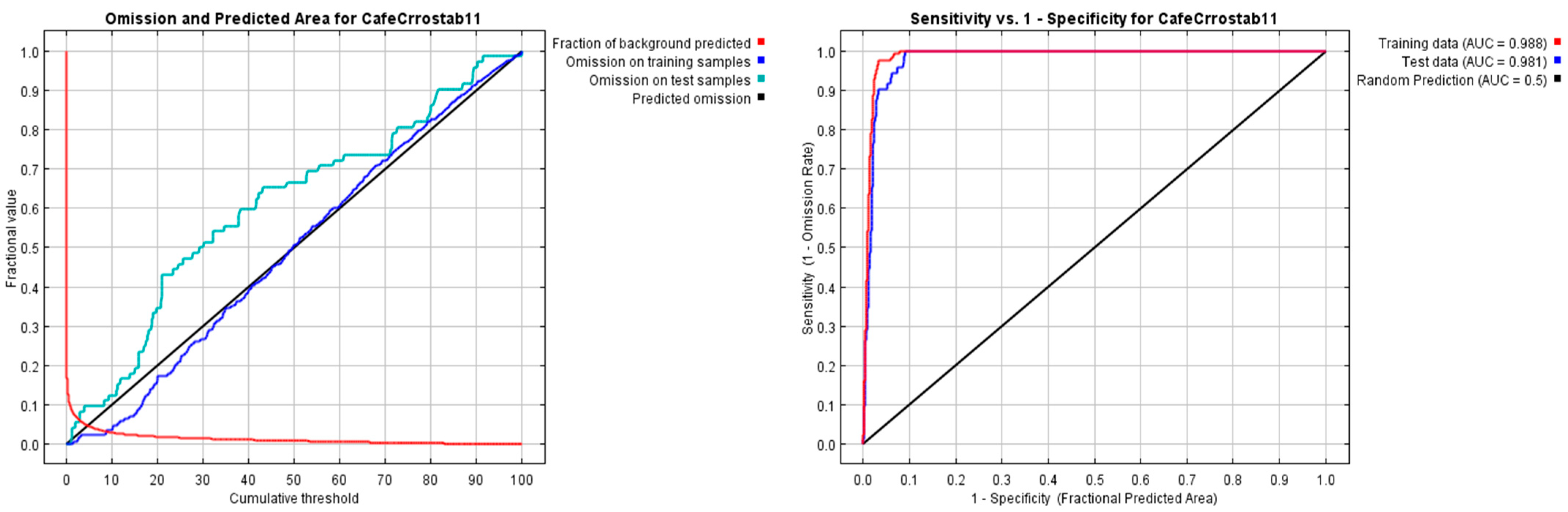
Figure 3 shows the sensitivity and specificity graph that quantifies the degree of fit of the model in the AUC value, indicating a model fit with a value of 99% in the training data and 98% for the test data, which was determined as an excellent model for predicting suitable habitats for the cultivation of the species [21].
The MaxEnt model was executed from the presence data with the biophysical variables, allowed generation of Table 3, which indicates the percentage contribution of each of the variables after running the jackknife test. The variable bio18, precipitation of the warmest quarter, has the highest contribution in the model with almost 33%, followed by bio3, isothermality, with 32% and bio23 with almost 13%, which together determine 77% of the contribution to the model.
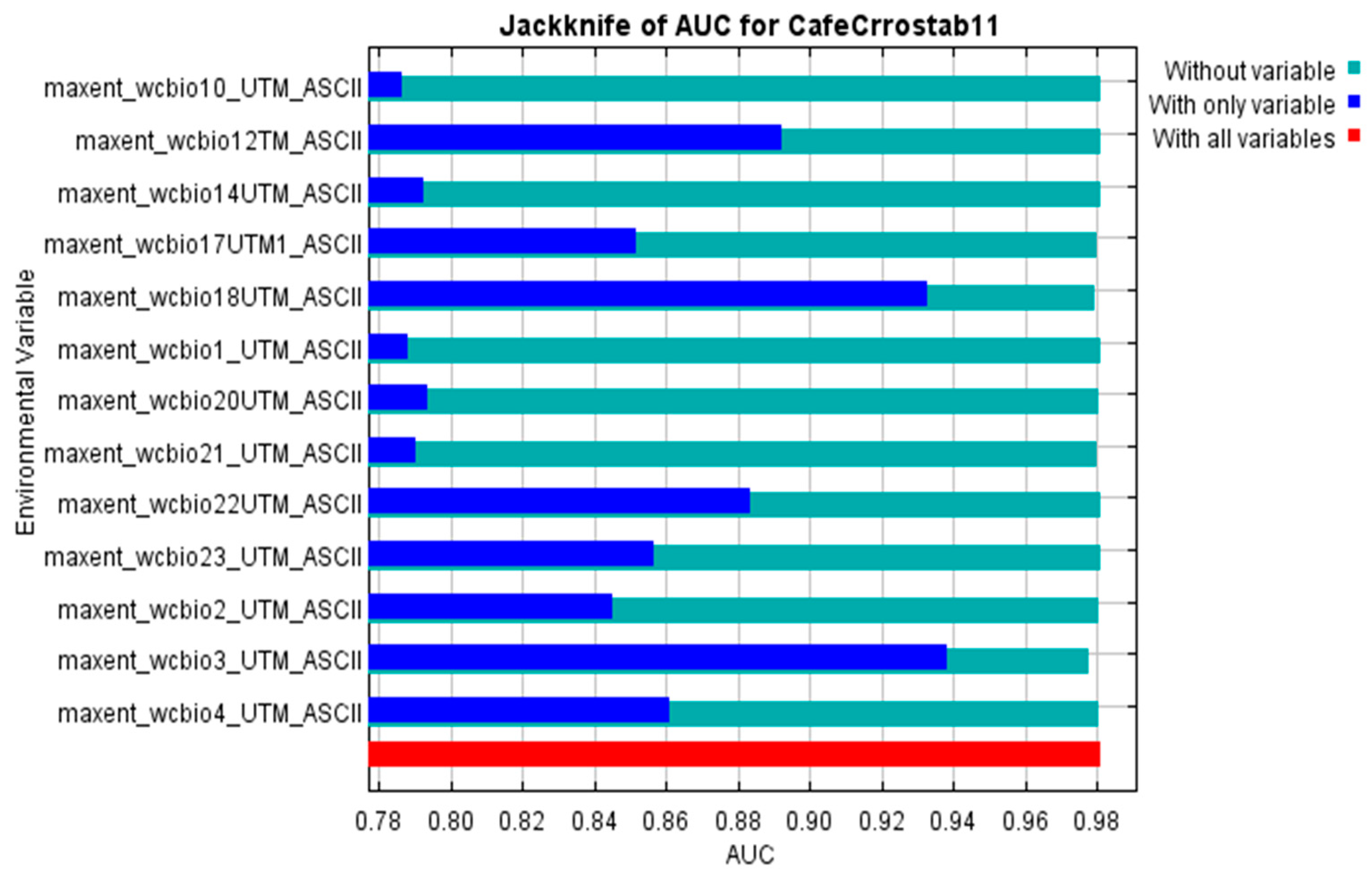
This information is complemented with Figure 4, which shows the jackknife test indicating the contribution of each of the variables by itself and with respect to the performance of the model without/with the same variable. This was able to determine that most of the variables behave in a similar way except for bio3, which is the one that negatively affects the performance of the model (decreases the level of certainty of the model).
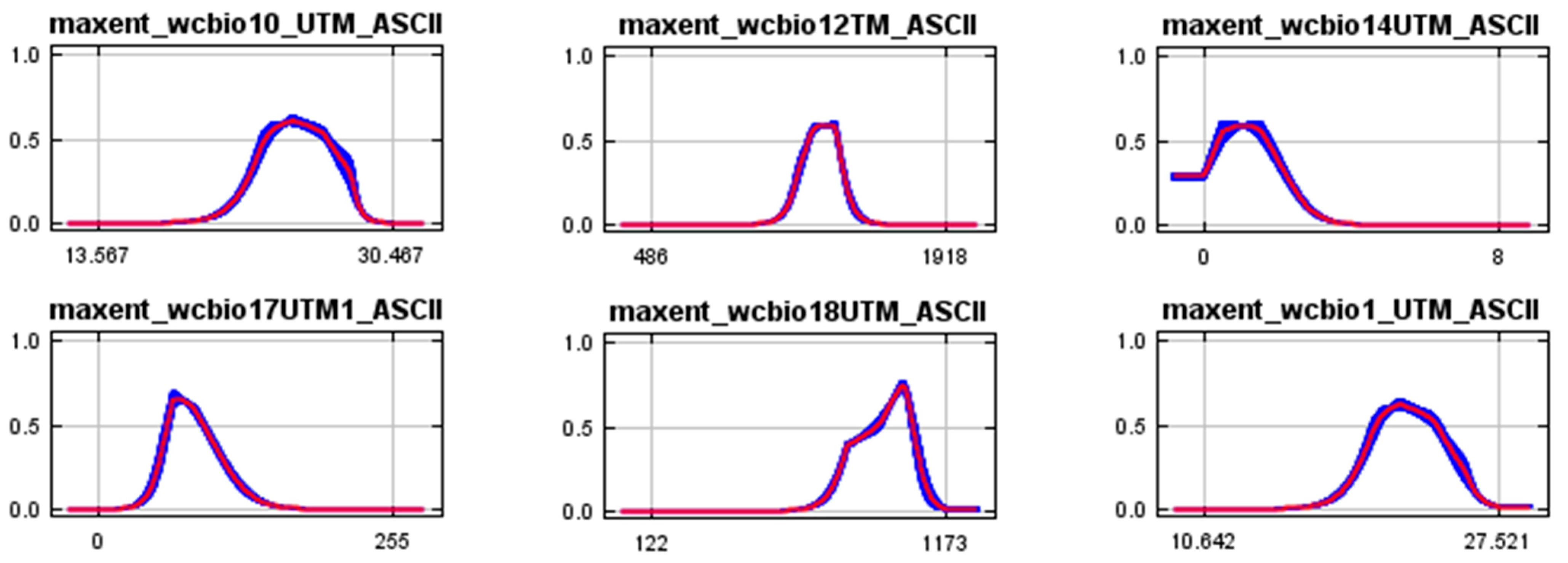
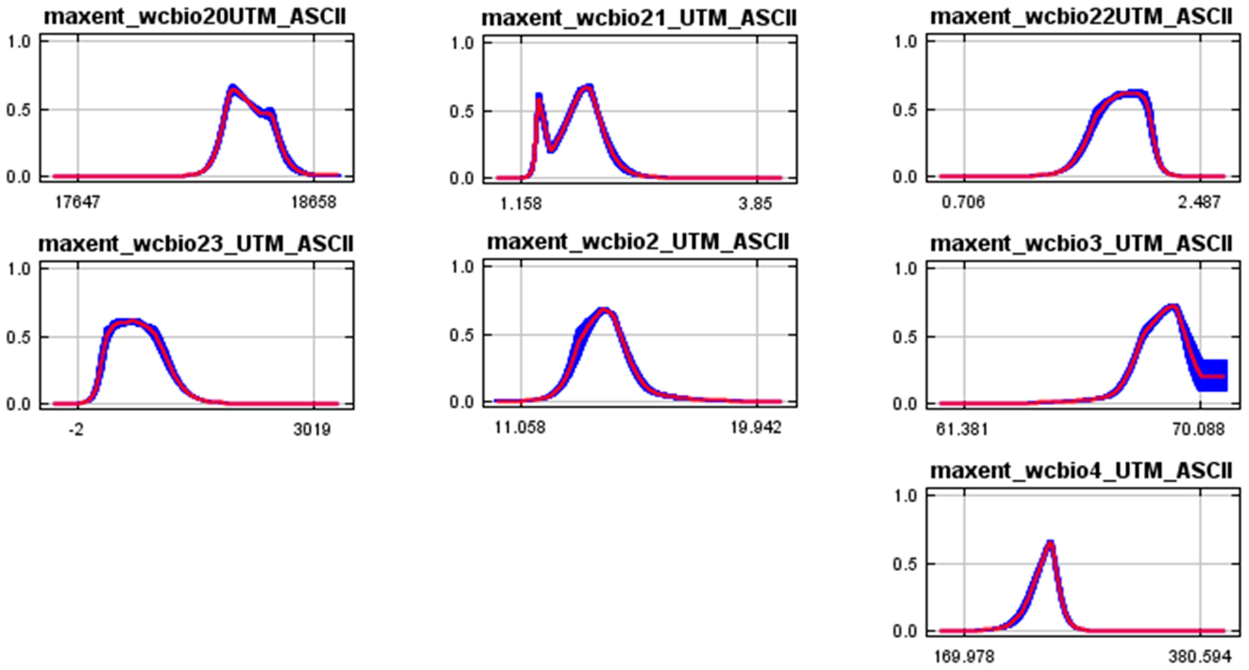
The results of the jackknife evaluation yield the response curves of Figure 5, where only the variables with values greater than 10% of the model contribution are considered. It particularly indicates that the precipitation variable of the warmest quarter (bio18) determines that the probability of occurrence increases in places with high rainfall in the warmest quarter; that is, in the rainy season, for its part, bio3 implies that the probability of occurrence increases the higher the isothermal interval; that is, the species prefers sites with high thermal variation throughout the day and night.
From the response curves, it is possible to infer the ranges of the maximum probability values that are detailed in Table 4 and that define the behavior of the variables in determining the ideal habitat for coffee production.
Potential Distribution Model (PDM)
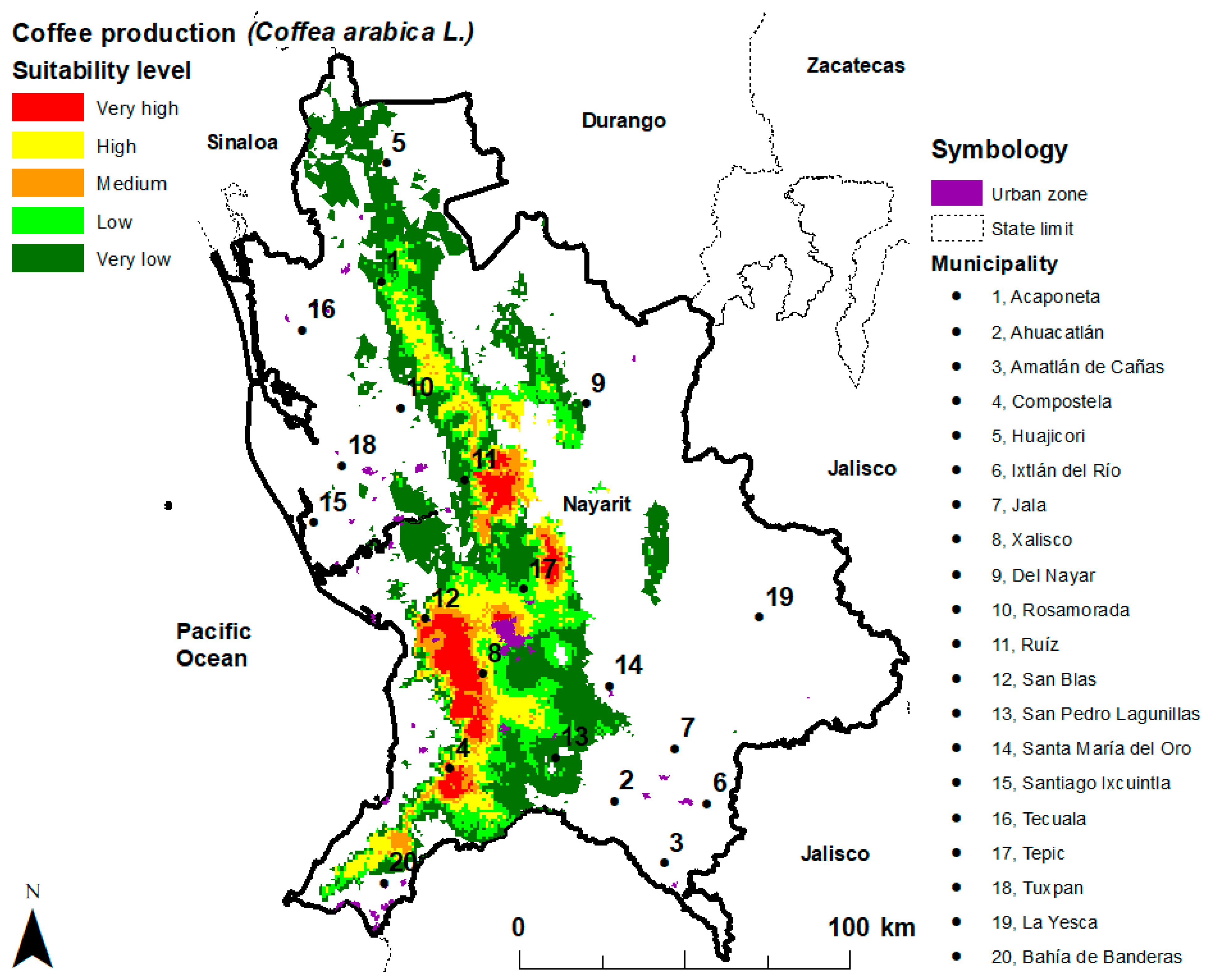
The distribution model indicated in Figure 6 shows the probability of finding suitable habitat for the specie; the red color indicates a high probability of having adequate conditions for the cultivation and production of coffee; the orange and green colors show the typical conditions of those sites, in which there is a probability of cultivation of the species; and the light green tones indicate a low probability predicted to find the conditions.
The generated model predicts that the suitability conditions are highly probable in the central region (vertically, crossing the state from north to south), represented by the Municipality of Tepic, Xalisco, the eastern area of Compostela, and the southwest of San Blas, where the prevailing conditions are a precipitation of the warmest quarter in the range of 1000 to 1010 mm, an isothermality of 68.3 to 69.2, and an altitude level in the range of 600 to 1000 m above sea level, as well as the other variables analyzed, whose preference ranges are described in Table 3. In general, the areas identified by the model correspond to hills and mountains, mainly from the sub-province’s physiographic sierras and northern plains, the neovolcanic sierras of Nayarit, and the sierra of the coast of Jalisco and Colima, in the physiographic provinces Sierra Madre Occidental, Eje Neovolcánico, and Sierra Madre del Sur, where different reference groups of soils predominate such as Luvisol, Cambisol, Regosol, Leptosol, Andosol, and Umbrisol.
Table 5 shows the conditions that prevail in each of the municipalities of the state of Nayarit with respect to surface suitability for coffee production, particularly highlighting the municipalities of Compostela with 27% and Xalisco (25%), the highest proportions of surfaces with very high suitability, although the municipality of Tepic can also be rescued as it reaches a surface of up to 24% with high suitability; on the other hand, the Municipalities of Amatlán de Cañas and Ixtlán del Río have no area of coffee productivity.
4. Discussion
Coffee (Coffea arabica L.) is a shrubby plant of the genus Rubiaceae and its natural distribution in space is associated with its tropical origin [81], so it is commonly distributed in the regions between the Tropic of Cancer at 23°27′ N. latitude and the Tropic of Capricorn at 23°26’ S. latitude from the Equator in areas characterized by conditions of high solar radiation and altitude ranges between 1300 and 1800 m.a.s.l., with temperatures between 17 and 23 °C [82]; however, due to the genetic composition and the great variety of species, some have the capacity to respond better or worse to certain environmental conditions, adapting to different ecosystems ranging from tropical rainforest to pine-oak forests, low deciduous forests, mesophilic mountain forests [83], and tropical evergreen forest [10]. A couple of studies were identified in the scientific literature, such as those of [31,32], which tried to identify how different variables impact the determination of the habitat of some species; however, for coffee, these types of analysis were not identified.
The factors that are associated with coffee production have been classified into two groups [3,84,85]: environmental, which generate the appropriate conditions for its development; and, agro-genetic, whose characteristics determine the quality of reproduction. In the present document, only the environmental variables are addressed in order to identify how these factors determine the distribution of the conditions of suitability of the habitat for coffee production. The factors that affect the distribution of the coffee species in Mexico have been identified by some authors such as [3], who point out that coffee is distributed on steep terrain in mountainous areas with rugged topography and high slopes, coinciding with areas of greater biological diversity, where the factors associated with the sites correspond to higher altitude, available humidity, frost, and soil with higher organic matter content.
On the other hand, in Mexico, [7] point out that the productive zones are located in mountainous areas of rugged topography and coincide with the places of greatest biological diversity in the country, especially in mountain cultivation systems.
In the same way, ref. [86] indicated that coffee production is more successful when it is cultivated at altitudes ranging from 600 to 1200 m above sea level, especially on steep slopes and in the transition zone between tropical and temperate ecosystems; likewise, [87] indicated that coffee flowering is influenced by environmental factors such as solar radiation, temperature, and availability of water in the soil. Likewise, [88] estimates that for coffee to develop and produce, appropriate climatic conditions are required of between 1500 and 2500 mm of average annual precipitation, without frost or prolonged droughts, and an altitude of between 600 and 1200 m, the same altitude. Similarly, ref. [89] mentions that the climatic requirements that influence the physical quality of coffee are a precipitation of between 1000 and 2500 mm per year, a temperature of between 17 and 24 °C, and relative humidity of 55 to 65%, in addition to an exposure of more than 1000 h of light per year and an altitude of 1200 to 2000 m above sea level.
In Nayarit, [90] points out that the coffee-productive regions are characterized by an irregular topography with steep slopes, fertile soils, richness in organic matter, and shallowness with lush vegetation in jungles, mountains and sub-deciduous forests with an average annual temperature of 24 °C and rainfall of 1200 mm annually.
All the works previously reviewed and cited here consider factors such as altitude, solar radiation, precipitation, temperature, and some others with ranges that differ relatively little among them as those that condition the suitability of the regions for optimum coffee production; however, none of them make reference to the analysis of influence and much less to the valuation of the contribution that each factor has in determining the environmentally suitable conditions. This situation is addressed with the present work in such a way that it contributes to determining the degree of influence that each one of the factors has on the presence of coffee, and, from the analysis of this association, it generates a Potential Distribution Model (PDM) that shows the ideal zones for the production of coffee.
In this sense, the results obtained in the present work indicate that the main environmental factors that contribute to establish the suitability of the zones for coffee production in Nayarit are isothermality, precipitation, and altitude, which partially coincides with what was indicated by the previously mentioned authors, since it is particularly found that precipitation is one of the variables that contributes the most to the model, especially in a range of 1000 to 1010 mm, with an isothermality of 68.3 to 69.2 and an altitude in the range of 600 to 1000 m.a.s.l.
On the other hand, although the MaxEnt model has demonstrated its efficiency in the modeling of the ecological niche, some authors have indicated some recommendations that should be considered and complied with prior to the execution of MaxEnt; in the first place, it should be considered that the accuracy of the presence data will have a significant impact on the degree of model fit [91]. In this sense, the selection of the variables used in this work is not intended to be limiting or definitive for the determination of the model, since other variables that could contribute to improve the model response can be analyzed. Another important assumption is related to the fact that there must be a temporal correspondence between the presence records of the observed species and the biophysical variables [92]. Likewise, the biophysical variables must affect the distribution of the species in such a way that they have a statistically significant influence on the presence of the species [93]; the latter because the appropriate selection of variables will determine the degree of model fit at larger scales once the model is generalized to other regions outside the study area [21].
5. Conclusions
In the present work, the SDM allowed for obtaining a first and good approximation of the potentially ideal habitat for coffee production in the state of Nayarit, being defined by the region comprised by the Municipality of Tepic, Xalisco, the eastern zone of Compostela, and the southwest of San Blas. The distribution model obtained adequately predicts the ideal zones for coffee production with a level of certainty of 98% (AUC = 0.98), and therefore represents a reliable model for the zoning of areas of importance for the coffee sector.
An area of 8182 km2 that is equivalent to approximately 30% of the surface of the territory of Nayarit has ideal conditions for coffee production, especially the landscapes of the lomerios and sierras of the Sierra Madre Occidental, Eje Neovolcánico, and Sierra Madre del Sur, in the municipalities of Tepic and Xalisco and the eastern zone of Compostela and southwest of San Blas, which should be considered as a Priority Conservation Area (PCA) for coffee production in the state.
The information resulting from the present research intends to lay the foundations for the diagnosis of coffee productivity zoning in Nayarit as knowledge that can be used by the governors to identify the zones with coffee production potential; and, secondly, to help establish planning strategies focused on managing, improving, and increasing production with a sustainable approach. The present model is also intended to be used for future work on the identification of biological corridors in order to promote tourism, as well as for further work on prediction and analysis of scenarios in the face of climate change and to see how the suitability conditions of the territory will be affected by the effect of variations of the different environmental variables.
The generation of knowledge on the identification of regions with ideal environmental conditions for coffee production in the state and the conservation strategies that are applied to them will allow generating, in the long term, the recognition of the quality of origin that the region offers.
Author Contributions
A.A.J. designed, developed the methodology of, and wrote this research paper. S.M.L.M.F., O.N.G. and F.F.V. reviewed and analyzed the data and approved the results obtained. All authors have read and agreed to the published version of the manuscript.
Funding
This research received no external funding.
Institutional Review Board Statement
Not applicable.
Informed Consent Statement
Not applicable.
Data Availability Statement
Not applicable.
Acknowledgments
The authors thank the Universidad Autónoma de Nayarit (UAN) for the support granted to the research project SIP22-128 “Retos y oportunidades en jóvenes cafetaleros: Estudio comparativo Colombia, México, Perú y Brasil”, of which this work is a part, as well as the register of coffee producers in the state of Nayarit for the information provided.
Conflicts of Interest
The authors declare no conflict of interest.
References
- OIC. Organización Internacional del Café (OIC). Available online: https://www.cancilleria.gov.co/international/multilateral/inter-governmental/ico (accessed on 20 November 2022).
- CDERSSA. Centro de Estudios para el Desarrollo Rural Sustentable y la Soberanía Alimentaria. Reporte el Café en México Diagnóstico y Perspectiva. 2018. Available online: http://www.cedrssa.gob.mx/ (accessed on 20 November 2022).
- Rosas, A.J.; Escamilla, P.E.; Ruiz, R.O. Relación de los nutrimentos del suelo con las características físicas y sensoriales del café orgánico. Terra Latinoam. 2008, 26, 375–384. Available online: http://www.scielo.org.mx/scielo.php?pid=S0187-57792008000400010&script=sci_arttext (accessed on 10 December 2022).
- Rivera, R.C.R. Competitiveness of the Mexican coffee in international trade: A comparative analysis with Brazil, Colombia, and Peru (2000–2019). Análisis Econ. 2022, 37, 181–199. [Google Scholar] [CrossRef]
- Nguyen, T.H.N. The Competitiveness of Vietnamese Coffe into the EU Market. 2016. Available online: https://urn.fi/URN:NBN:fi:amk-201603303652 (accessed on 10 December 2022).
- Barrera, R.A.; Ramírez, G.A.G.; Cuevas, R.V.; y Espejel García, A. Modelos de innovación en la producción de café en la Sierra Norte de Puebla-México. Rev. Cienc. Soc. 2021, 26, 443–458. [Google Scholar] [CrossRef]
- Escamilla, P.; y Díaz, C.S. Sistemas de Cultivo de Café en México; Universidad Autónoma de Chapingo & Fundación Produce: Huatusco, México, 2002. [Google Scholar]
- Barrita-Ríos, E.E.; Espinosa-Trujillo, M.A.; Pérez-Vera, F.C.; Rentabilidad de Dos Sistemas de Producción de Café Cereza (Coffea Arábica L.) en Pluma Hidalgo, Oaxaca, México. Guía para Autores AGRO. 2018. Available online: https://core.ac.uk/download/pdf/249320086.pdf (accessed on 10 December 2022).
- Vichi, F.F. La producción de café en México: Ventana de oportunidad para el sector agrícola de Chiapas. Espac. Innovación Más Desarro. 2015, 4, 174–194. [Google Scholar] [CrossRef]
- García, M.L.E.; Valdez, H.J.I.; Luna, C.M.; López, M.R. Estructura y diversidad arbórea en sistemas agroforestales de café en la Sierra de Atoyac, Veracruz. Madera Bosques 2015, 21, 69–82. Available online: http://hdl.handle.net/10521/2379 (accessed on 20 November 2022).
- Vandermeer, J.H. The Coffee Agroecosystem in the Neotropics: Combining. Ecological. and. Economic. Goals. In Tropical Agroecosystems; CRC Press: Boca Raton, FL, USA, 2003; pp. 159–194. [Google Scholar]
- Richter, A.; Klein, A.M.; Tscharntke, T.; Tylianakis, J.M. Abandonement of coffee agroforests increases insect abundance and diversity. Agrofor. Syst. 2007, 69, 175–182. [Google Scholar] [CrossRef]
- Toledo, V.M.; Moguel, P. Coffee and sustainability: The multiple values of traditional shaded coffee. J. Sustain. Agric. 2012, 36, 353–377. [Google Scholar] [CrossRef]
- Beer, J.; Harvey, C.; Ibrahim, M.; Harmand, J.M.; Somarriba, E.; Jiménez, F. Servicios ambientales de los sistemas agroforestales. Agrofor. Am. 2003, 10, 80–87. Available online: https://repositorio.catie.ac.cr/handle/11554/6806 (accessed on 10 December 2022).
- Soto-Pinto, L.; Romero-Alvarado, Y.; Caballero-Nieto, J.; Segura Warnholtz, G. Woody plant diversity and structure of shade-grown-coffee plantations in Northern Chiapas, Mexico. Rev. Biol. Trop. 2001, 49, 977–987. Available online: https://www.scielo.sa.cr/scielo.php?pid=S0034-77442001000300018&script=sci_arttext (accessed on 20 November 2022).
- Pineda-López, M.; Ortiz-Ceballos, G.; Sánchez-Velásquez, L.R. Los cafetales y su papel en la captura de carbono: Un servicio ambiental aún no valorado en Veracruz. Madera Bosques 2005, 11, 3–14. [Google Scholar] [CrossRef]
- Roncal-García, S.; Soto-Pinto, L.; Castellanos-Albores, J.; Ramírez-Marcial, N.; De Jong, B. Sistemas agroforestales y almacenamiento de carbono en comunidades indígenas de Chiapas, México. Interciencia 2008, 33, 200–206. Available online: http://ve.scielo.org/scielo.php?script=sci_arttext&pid=S0378-18442008000300009 (accessed on 25 November 2022).
- Rhiney, K.; Guido, Z.; Knudson, C.; Avelino, J.; Bacon, C.M.; Leclerc, G.; Aime, M.C.; Bebber, D.P. Epidemics and the future of coffee production. Proc. Natl. Acad. Sci. USA 2021, 118, e2023212118. [Google Scholar] [CrossRef] [PubMed]
- Tamru, S.; Engida, E.; Minten, B. Impacts of the COVID-19 Crisis on Coffee Value Chains in Ethiopia. IFPRI. 2020. Available online: http://essp.ifpri.info/files/2020/04/coffee_blog_April_2020.pdf (accessed on 25 November 2022).
- Lopez-Ridaura, S.; Sanders, A.; Barba-Escoto, L.; Wiegel, J.; Mayorga-Cortes, M.; Gonzalez-Esquivel, C.; Lopez-Ramirez, M.A.; Escoto-Masis, R.M.; Morales-Galindo, E.; García-Barcena, T.S. Immediate impact of COVID-19 pandemic on farming systems in Central America and Mexico. Agric. Syst. 2021, 192, 103–178. [Google Scholar] [CrossRef]
- Phillips, S.J.; Anderson, R.P.; Schapire, R.E. Maximum entropy modeling of species geographic distributions. Ecol. Model. 2006, 190, 231–259. [Google Scholar] [CrossRef] [Green Version]
- Espinosa, C.C.; Trigo, T.C.; Tirelli, F.P.; da Silva, L.G.; Eizirik, E.; Queirolo, D.; Mazim, F.D.; Peters, F.B.; Favarini, M.O.; de Freitas, T.R. Geographic distribution modeling of the margay (Leopardus wiedii) and jaguarundi (Puma yagouaroundi): A comparative assessment. J. Mammal. 2018, 99, 252–262. [Google Scholar] [CrossRef] [Green Version]
- Martínez-Méndez, N.; Aguirre-Planter, E.; Eguiarte, L.E.; Jaramillo-Correa, J.P. Modelado de nicho ecológico de las especies del género Abies (Pinaceae) en México: Algunas implicaciones taxonómicas y para la conservación. Bot. Sci. 2016, 94, 5–24. [Google Scholar] [CrossRef] [Green Version]
- Illoldi-Rangel, P.; Escalante, T. De los modelos de nicho ecológico a las áreas de distribución geográfica. Biogeografía 2008, 3, 7–12. [Google Scholar]
- Li, Y.; Cao, W.; He, X.; Chen, W.; Xu, S. Prediction of Suitable Habitat for Lycophytes and Ferns in Northeast China: A Case Study on Athyrium brevifrons. Chin. Geogr. Sci. 2019, 29, 1011–1023. [Google Scholar] [CrossRef] [Green Version]
- Ghareghan, F.; Ghanbarian, G.; Pourghasemi, H.R.; Safaeian, R. Prediction of habitat suitability of Morina persica L. species using artificial intelligence techniques. Ecol. Indic. 2020, 112, 106096. [Google Scholar] [CrossRef]
- Pérez, M.R.; Romero, S.M.E.; González, H.A.; Pérez, S.E.; Arriola, P.V.J. Distribución potencial de Lophodermium spp. en bosques de coníferas, con escenarios de cambio climático. Rev. Mex. Cienc. For. 2016, 7, 81–97. [Google Scholar] [CrossRef] [Green Version]
- Javed, S.M.; Raj, M.; Kumar, S. Predicting Potential Habitat Suitability for an Endemic Gecko Calodactylodes aureus and its Conservation Implications in India. Trop. Ecol. 2017, 58, 271–282. Available online: http://216.10.241.130/pdf/open/PDF_58_2/5/5.%20Javed%20et%20al.pdf (accessed on 20 November 2022).
- Phillips, S.J.; Dudík, M.; Schapire, R.E. A maximum entropy approach to species distribution modeling. In Proceedings of the Twenty-First International Conference on Machine learning, Alberta, Canada, 4–8 July 2004; pp. 1–83. [Google Scholar] [CrossRef] [Green Version]
- Promnun, P.; Kongrit, C.; Tandavanitj, N.; Techachoochert, S.; Khudamrongsawat, J. Predicting potential distribution of an endemic butterfly lizard, Leiolepis ocellata (Squamata: Agamidae). Trop. Nat. Hist. 2020, 20, 60–71. Available online: https://li01.tci-thaijo.org/index.php/tnh/article/view/198819 (accessed on 25 November 2022).
- Thakur, D.; Rathore, N.; Sharma, M.K.; Parkash, O.; Chawla, A. Identification of ecological factors affecting the occurrence and abundance of Dactylorhiza hatagirea (D. Don) Soo in the Himalaya. J. Appl. Res. Med. Aromat. Plants 2021, 20, 100286. [Google Scholar] [CrossRef]
- De Sousa, G.J.A.; de Souza, B.I.; Paiva, L.R.F.; Souza, R.S.; Bezerra, G.L. Modeling and potential distribution of tree species relevant to the sociocultural and ecological dynamics in the Sete Cidades National Park, Piauí, Brazil. Soc. Nat. 2022, 32, 784–798. [Google Scholar] [CrossRef]
- Ab Lah, N.Z.; Yusop, Z.; Hashim, M.; Mohd Salim, J.; Numata, S. Predicting the Habitat Suitability of Melaleuca cajuputi Based on the MaxEnt Species Distribution Model. Forests 2021, 12, 1449. [Google Scholar] [CrossRef]
- Chhetri, P.K.; Gaddis, K.D.; Cairns, D.M. Predicting the suitable habitat of treeline species in the Nepalese Himalayas under climate change. Mt. Res. Dev. 2018, 38, 153–163. [Google Scholar] [CrossRef] [Green Version]
- Tesfamariam, B.G.; Gessesse, B.; Melgani, F. MaxEnt-based modeling of suitable habitat for rehabilitation of Podocarpus forest at landscape-scale. Environ. Syst. Res. 2022, 11, 4. [Google Scholar] [CrossRef]
- Kamyo, T.; Asanok, L. Modeling habitat suitability of Dipterocarpus alatus (Dipterocarpaceae) using maxent along the chao phraya river in central Thailand. For. Sci. Technol. 2020, 16, 1–7. [Google Scholar] [CrossRef] [Green Version]
- Yang, J.; Jiang, P.; Huang, Y.; Yang, Y.; Wang, R.; Yang, Y. Potential geographic distribution of relict plant Pteroceltis tatarinowii in China under climate change scenarios. PLoS ONE 2022, 17, e0266133. [Google Scholar] [CrossRef]
- Singh, P.; Saran, S.; Kocaman, S. Role of Maximum Entropy and Citizen Science to Study Habitat Suitability of Jacobin Cuckoo in Different Climate Change Scenarios. Int. J. Geo-Inf. 2021, 10, 463. [Google Scholar] [CrossRef]
- Boral, D.; Moktan, S. Predictive distribution modeling of Swertia bimaculata in Darjeeling-Sikkim Eastern Himalaya using MaxEnt: Current and future scenarios. Ecol. Process. 2021, 10, 26. [Google Scholar] [CrossRef]
- Thapa, S.; Baral, S.; Hu, Y.; Huang, Z.; Yue, Y.; Dhakal, M.; Jnawali, S.R.; Chettri, N.; Racey, P.A.; Wu, Y. Will climate change impact distribution of bats in Nepal Himalayas? A case study of five species. Glob. Ecol. Conserv. 2021, 26, e01483. [Google Scholar] [CrossRef]
- Mishra, S.N.; Gupta, H.S.; Kulkarni, N. Impact of climate change on the distribution of Sal species. Ecol. Inform. 2021, 61, 1–12. [Google Scholar] [CrossRef]
- Ning, S.N.; Naudiyal, N.; Wang, J.; Gaire, N.P.; Wu, Y.; Wei, Y.; He, J.; Wang, C. Assessing the Impact of Climate Change on Potential Distribution of Meconopsis punicea and Its Influence on Ecosystem Services Supply in the Southeastern Margin of Qinghai-Tibet Plateau. Front. Plant Sci. 2022, 12, 830119. [Google Scholar] [CrossRef]
- Tang, X.; Yuan, Y.; Li, X.; Zhang, J. Maximum entropy modeling to predict the impact of climate change on pine wilt disease in China. Front. Plant Sci. 2021, 12, 652500. [Google Scholar] [CrossRef]
- Wan, J.N.; Mbari, N.J.; Wang, S.W.; Liu, B.; Mwangi, B.N.; Rasoarahona, J.R.; Xin, H.-P.; Zhou, Y.-D.; Wang, Q.F. Modeling impacts of climate change on the potential distribution of six endemic baobab species in Madagascar. Plant Divers. 2021, 43, 117–124. [Google Scholar] [CrossRef]
- Setyawan, A.D.; Supriatna, J.; Nisyawati, N.; Nursamsi, I.; Sutarno, S.; Sugiyarto, S.; Sunarto, S.; Pradan, P.; Budiharta, S.; Pitoyo, A.; et al. Predicting potential impacts of climate change on the geographical distribution of mountainous selaginellas in Java, Indonesia. Biodiversitas J. Biol. Divers. 2020, 21, 2252–2269. [Google Scholar] [CrossRef]
- Wang, F.; Wang, D.; Guo, G.; Zhang, M.; Lang, J.; Wei, J. Potential distributions of the invasive barnacle scale Ceroplastes cirripediformis (Hemiptera: Coccidae) under climate change and implications for its management. J. Econ. Entomol. 2021, 114, 82–89. [Google Scholar] [CrossRef]
- Alatawi, A.S.; Gilbert, F.; Reader, T. Modelling terrestrial reptile species richness, distributions and habitat suitability in Saudi Arabia. J. Arid. Environ. 2020, 178, 104153. [Google Scholar] [CrossRef]
- Warren, D.L.; Seifert, S.N. Ecological niche modeling in Maxent: The importance of model complexity and the performance of model selection criteria. Ecol. Appl. 2011, 21, 335–342. [Google Scholar] [CrossRef] [Green Version]
- Tang, J.; Li, J.; Lu, H.; Lu, F.; Lu, B. Potential distribution of an invasive pest, Eu platypus parallelus, in China as predicted by Maxent. Pest Manag. Sci. 2019, 75, 1630–1637. [Google Scholar] [CrossRef] [PubMed]
- Fand, B.B.; Shashank, P.R.; Suroshe, S.S.; Chandrashekar, K.; Meshram, N.M.; Timmanna, H.N. Invasion risk of the South American tomato pinworm Tuta absoluta (Meyrick) (Lepidoptera: Gelechiidae) in India: Predictions based on MaxEnt ecological niche modelling. Int. J. Trop. Insect. Sci. 2020, 40, 561–571. [Google Scholar] [CrossRef]
- Mushtaq, S.; Reshi, Z.A.; Shah, M.A.; Charles, B. Modelled distribution of an invasive alien plant species differs at different spatiotemporal scales under changing climate: A case study of Parthenium hysterophorus L. Trop. Ecol. 2021, 62, 398–417. [Google Scholar] [CrossRef]
- Kumar, S.; Stohlgren, T.J. Maxent modeling for predicting suitable habitat for threatened and endangered tree Canacomyrica monticola in New Caledonia. J. Ecol. Nat. Environ. 2009, 1, 94–98. Available online: https://academicjournals.org/journal/JENE/article-full-text-pdf/C1CDB822968 (accessed on 20 November 2022).
- Aroca-Gonzalez, B.D.; Gradstein, R.; González-Nieves, L.M. ¿En peligro o no? Distribución potencial de la hepática Pleurozia paradoxa en Colombia. Rev. Acad. Colomb. Cienc. Exactas Físicas Nat. 2021, 45, 260–271. [Google Scholar] [CrossRef]
- Ordoñez-Sierra, R.; Mastachi-Loza, C.A.; Díaz-Delgado, C.; Cuervo-Robayo, A.P.; Fonseca Ortiz, C.R.; Gómez-Albores, M.A.; Medina Torres, I. Spatial Risk Distribution of Dengue Based on the Ecological Niche Model of Aedes aegypti (Diptera: Culicidae) in the Central Mexican Highlands. J. Med. Entomol. 2020, 57, 728–737. [Google Scholar] [CrossRef]
- Martínez-Sifuentes, A.R.; Villanueva-Díaz, J.; Manzanilla-Quiñones, U.; Becerra-López, J.L.; Hernández-Herrera, J.A.; Estrada-Ávalos, J.; Velázquez-Pérez, A.H. Spatial modeling of the ecological niche of Pinus greggii Engelm (Pinaceae): A species conservation proposal in Mexico under climatic change scenarios. Iforest-Biogeosci. For. 2020, 13, 426–434. [Google Scholar] [CrossRef]
- Rodríguez-Soto, C.; Monroy-Vilchis, O.; Maiorano, L.; Boitani, L.; Faller, J.C.; Briones, M.A.; Núñez, R.; Rosas-Rosas, O.; Ceballos, G.; Falcucci, A. Predicting potential distribution of the jaguar (Panthera onca) in Mexico: Identification of priority areas for conservation. Divers. Distrib. 2011, 17, 350–361. [Google Scholar] [CrossRef]
- Cupul-Magaña, F.G.; Flores-Guerrero, U.S.; Escobedo-Galván, A.H. Distribución potencial de la tortuga mesoamericana Trachemys ornata en México Potential distribution of ornate slider Trachemys ornata in Mexico. Nota Científica 2020, 15, 1–124. [Google Scholar] [CrossRef]
- Aceves-Rangel, L.D.; Méndez-González, J.; García-Aranda, M.A.; Nájera-Luna, J.A. Distribución potencial de 20 especies de pinos en México. Agrociencia 2018, 52, 1043–1057. Available online: https://agrociencia-colpos.mx/index.php/agrociencia/article/view/1721 (accessed on 25 November 2022).
- Ibarra-Montoya, J.L.; Rangel-Peraza, G.; González-Farias, F.A.; De Anda, J.; Martínez-Meyer, E.; Macias-Cuellar, H. Uso del modelado de nicho ecológico como una herramienta para predecir la distribución potencial de Microcystis sp (cianobacteria) en la Presa Hidroeléctrica de Aguamilpa, Nayarit, México. Rev. Ambiente Água 2012, 7, 218–234. [Google Scholar] [CrossRef]
- Ibarra-Montoya, J.L.; Rangel-Peraza, G.; González-Farias, F.A.; De Anda, J.; Zamudio-Reséndiz, M.E.; Martínez-Meyer, E.; Macias-Cuellar, H. Modelo de nicho ecológico para predecir la distribución potencial de fitoplancton en la Presa Hidroeléctrica Aguamilpa, Nayarit. México. Ambiente Água-Interdiscip. J. Appl. Sci. 2010, 5, 60–75. [Google Scholar] [CrossRef]
- Garibay-Castro, L.R.; Gutiérrez-Yurrita, P.J.; López-Laredo, A.R.; Hernández-Ruíz, J.; Trejo-Espino, J.L. Potential Distribution and Medicinal Uses of the Mexican Plant Cuphea aequipetala Cav. (Lythraceae). Diversity 2022, 14, 403. [Google Scholar] [CrossRef]
- Medina-Amaya, M.; Ruiz-Gómez, M.G.; Gómez Díaz, J.A. Análisis de la distribución de Cedrela salvadorensis Standl. (Meliaceae) e implicaciones para su conservación. Gayana. Bot. 2021, 78, 172–183. [Google Scholar] [CrossRef]
- Martínez-Villagomez, M. Diversidad y distribución del género Persea Mill., en México. Agro Productividad 2018, 9. Available online: https://www.revista-agroproductividad.org/index.php/agroproductividad/article/view/750 (accessed on 20 November 2022).
- INEGI. Instituto Nacional de Estadística y Geografía (INEGI). 2020. Available online: https://www.inegi.org.mx/ (accessed on 20 November 2022).
- SIAP. Servicio de Información Agroalimentaria y Pesquera. 2020. Available online: https://www.gob.mx/siap (accessed on 10 December 2022).
- R Core Team. R: A Language and Environment for Statistical Computing; R Foundation for Statistical Computing: Vienna, Austria, 2020; Available online: https://www.R-project.org/ (accessed on 10 December 2022).
- Baldwin, R.A. Use of maximum entropy modeling in wildlife research. Entropy 2009, 11, 854–866. [Google Scholar] [CrossRef]
- Phillips, S.J. Transferability, sample selection bias and background data in presence-only modelling: A response to Peterson et al. Ecography 2008, 31, 272–278. Available online: https://www.jstor.org/stable/30244574 (accessed on 20 November 2022). [CrossRef]
- Elith, J.; Graham, C.H.; Anderson, R.P.; Dudik, M.; Ferrier, S. Novel methods improve prediction of species distributions from occurrence data. Ecography 2006, 29, 129–151. [Google Scholar] [CrossRef] [Green Version]
- Phipps, W.L.; Diekmann, M.; MacTavish, L.M.; Mendelsohn, J.M.; Naidoo, V.; Wolter, K.; Yarnell, R.W. Due South: A first assessment of the potential impacts of climate change on Cape vulture occurrence. Biol. Conserv. 2017, 210, 16–25. [Google Scholar] [CrossRef] [Green Version]
- Fielding, A.H.; Bell, J.F. A review of methods for the assessment of prediction errors in conservation presence-absence models. Environ. Conserv. 1997, 24, 38–49. [Google Scholar] [CrossRef]
- Merow, C.; Smith, M.J.; Silander, J.A., Jr. A practical guide to MaxEnt for modeling species’ distributions: What it does, and why inputs and settings matter. Ecography 2013, 36, 1058–1069. [Google Scholar] [CrossRef]
- Li, S.; Wang, Z.; Zhu, Z.; Tao, Y.; Xiang, J. Predicting the potential suitable distribution area of Emeia pseudosauteri in Zhejiang Province based on the MaxEnt model. Sci. Rep. 2023, 13, 1806. [Google Scholar] [CrossRef] [PubMed]
- Allouche, O.; Tsoar, A.; Kadmon, R. Assessing the accuracy of species distribution models: Prevalence, kappa and the true skill statistic (TSS). J. Appl. Ecol. 2006, 43, 1223–1232. [Google Scholar] [CrossRef]
- Wang, Y.; Xie, B.; Wan, F.; Xiao, Q.; Dai, L. Application of ROC curve analysis in evaluating the performance of alien species’ potential distribution models. Biodivers. Sci. 2007, 15, 365–372. Available online: https://www.biodiversity-science.net/EN/10.1360/biodiv.060280 (accessed on 10 December 2022).
- Peterson, A.T.; Soberón, J.; Pearson, R.G.; Anderson, R.P.; Martínez-Meyer, E.; Nakamura, M. Ecological Niches and Geographic Distributions. Monographs in Population Biology, 49; Princeton University Press: Princeton, NJ, USA, 2011. [Google Scholar] [CrossRef]
- Vilar, L.; Gómez, I.; Martínez-Vega, J.; Echavarría, P.; Riaño, D.; Martín, M.P. Multitemporal modelling of socio-economic wildfire drivers in central Spain between the 1980s and the 2000s: Comparing generalized linear models to machine learning algorithms. PLoS ONE 2016, 11, e0161344. [Google Scholar] [CrossRef] [Green Version]
- Préau, C.; Trochet, A.; Bertrand, R.; Isselin-Nondereu, F. Modeling potential distributions of three European amphibian species comparing ENFA and Maxent. Herpetol. Conserv. Biol. 2018, 13, 91–104. [Google Scholar]
- Qin, A.; Jin, K.; Batsaikhan, M.E.; Nyamjav, J.; Li, G.; Li, J.; Xue, Y.; Sun, G.; Wu, L.; Indree, T.; et al. Predicting the current and future suitable habitats of the main dietary plants of the Gobi Bear using MaxEnt modeling. Glob. Ecol. Conserv. 2020, 22, e01032. [Google Scholar] [CrossRef]
- Porfirio, L.L.; Harris, R.M.; Lefroy, E.C.; Hugh, S.; Gould, S.F.; Lee, G.; Bindoff, N.L.; Mackey, B. Improving the use of species distribution models in conservation planning and management under climate change. PLoS ONE 2014, 9, e113749. [Google Scholar] [CrossRef] [Green Version]
- Toledo, V.M.; y Moguel, P. El café en México, Ecología, Cultura Indígena y Sustentabilidad. Ciencias 1996, 43, 40–51. Available online: http://www.ejournal.unam.mx/cns/no43/CNS04306.pdf?iframe=true&width=90%&height=90% (accessed on 10 December 2022).
- Chávez, J. «Asumiendo la vida con una taza de café». In Desafíos y Perspectivas de la Situación Ambiental en el Perú. En el Marco de la Conmemoración de los 200 Años de Vida Republicana; Castro, A., Merino-Gómez, M.I., Eds.; INTE-PUCP: Lima, Peru, 2022; pp. 226–245. [Google Scholar] [CrossRef]
- Moguel, P. Biodiversidad y cultivos agroindustriales: El caso del café. In Reporte Técnico Presentado a Comisión Nacional para el Conocimiento y Uso de la Biodiversidad (CONABIO); Instituto de Ecología, Universidad Nacional Autónoma de México (UNAM): México City, México, 1996. [Google Scholar]
- Santoyo Cortés, V.H.; Díaz Cárdenas, S. Sistema Agroindustrial Café en México: Diagnóstico, Problemática y Alternativas; Universidad Autonoma Chapingo: Chapingo, Mexico, 1994; No. 633.73 S35. [Google Scholar]
- Wintgens, J.N. Coffee: Growing, Processing, Sustainable Production. A Guidebook for Growers, Processors, Traders, and Researchers. 2004, pp. 1–976. Available online: https://www.cabdirect.org/cabdirect/abstract/20113026416 (accessed on 10 December 2022).
- Moguel, P.; Toledo, V.M. Biodiversity conservation in traditional coffee systems of Mexico. Conserv. Biol. 1999, 13, 11–21. [Google Scholar] [CrossRef]
- Vélez, B.E.; Jaramillo, A.; Cháves, B.; Franco, M. Distribución de la Floración y la Cosecha de Café en Tres Altitudes. Centro Nacional de Investigaciones de Café (Cenicafé). 2000. Available online: https://biblioteca.cenicafe.org/handle/10778/794 (accessed on 20 November 2022).
- Moguel, P.; Toledo, V.M. Conservar Produciendo: Biodiversidad, Café Orgánico. 2004. Available online: http://www.conabio.gob.mx/institucion/conabio_espanol/doctos/Biodiv55.pdf (accessed on 10 December 2022).
- Caviedes, F.M. Factores que Determinan la Calidad Física y Sensorial del Café. 2022. Available online: https://repositorio.sierraexportadora.gob.pe/bitstream/handle/SSE/448/FACTORES%20QUE%20DETERMINAN%20LA%20CALIDAD%20FISICO%20Y%20SENSORIAL%20EN%20EL%20CAFE.pdf?sequence=2&isAllowed=y (accessed on 10 December 2022).
- Mariscal, H.E.I.; Marceleño, F.S.; y Nájera, G.O. Análisis de la cadena productiva del café en el estado de Nayarit, México. Rev. Fac. Cienc. Contab. Econ. Adm. Faccea 2019, 9, 100–112. [Google Scholar] [CrossRef]
- Stockwell, D.R.; Peterson, A.T. Effects of sample size on accuracy of species distribution models. Ecol. Model. 2002, 148, 1–13. [Google Scholar] [CrossRef]
- Anderson, R.P.; Martınez-Meyer, E. Modeling species’ geographic distributions for preliminary conservation assessments: An implementation with the spiny pocket mice (Heteromys) of Ecuador. Biol. Conserv. 2004, 116, 167–179. [Google Scholar] [CrossRef]
- Pearson, R.G.; Raxworthy, C.J.; Nakamura, M.; Townsend, P. Predicting species distributions from small numbers of occurrence records: A test case using cryptic geckos in Madagascar. J. Biogeogr. 2006, 34, 102–117. [Google Scholar] [CrossRef]
Figure 1.
Location of the study area. Source: own elaboration. Has data from INEGI, (2019).

Figure 2.
Methodological process for obtaining the species potential distribution model.

Figure 3.
Omission and prediction curves of the model run in MaxEnt for the coffee specie.

Figure 4.
Jackknife test indicating contribution of variables.

Figure 5.
Response curves of the variables with values greater than 10% of the model’s contribution.
Figure 5.
Response curves of the variables with values greater than 10% of the model’s contribution.


Figure 6.
Map of distribution of probability of location of habitat zones with high suitability.


Table 1.
Coffee species presence and environmental variables used in the coffee distribution model.
| Factor | Component | Key | Variable | Description | Unit |
|---|---|---|---|---|---|
| Species | Coffe | Coffee presence records (Dependent variable) | Centroids of the areas where there is coffee production | - | |
| Climatic | Temperature | Bio1 | Average annual temperature | Represents the average temperature throughout the year | °C |
| Bio2 | Mean of the diurnal range. Monthly average (max temp–min temp) | Identifies diurnal temperature fluctuations | - | ||
| Bio3 | Isothermality (Bio2/Bio7)(×100) | Describes the magnitude of temperature swings between day and night relative to the annual temperature range | - | ||
| Bio4 | Temperature seasonality (Standard deviation ×100) | Indicates peak periods between temperature ranges | - | ||
| Bio5 | Maximum temperature of the warmest month | Represents the highest temperature in the warmest month | °C | ||
| Bio6 | Minimum temperature of the coldest month | Represents the lowest temperature in the coldest month | °C | ||
| Bio7 | Annual temperature range (Bio5-Bio6) | Shows the ranges of extreme temperature conditions | °C | ||
| Bio8 | Average temperature of the most humid room | Describes the average temperature of the quarter of the year with the highest humidity | °C | ||
| Bio9 | Average temperature of the driest quarter | Indicates the average temperature of the driest quarter of the year | °C | ||
| Bio10 | Average temperature of the warmest room | Describes the average temperature of the warmest quarter of the year | °C | ||
| Bio11 | Average temperature of the coldest room | Represents the average temperature of the coldest quarter of the year | °C | ||
| Precipitation | Bio12 | Annual precipitation | It represents the frequency and amount of rainwater that falls on a specific place throughout the year. | mm | |
| Bio13 | Rainfall of the wettest month | Represents the frequency and amount of rainfall falling on a specific location in the wettest month. | mm | ||
| Bio14 | Rainfall of the driest month | Represents the frequency and amount of rainfall falling on a specific location in the driest month. | mm | ||
| Bio15 | Precipitation seasonality (coefficient of variation) | Indicates periods of precipitation variation | - | ||
| Bio16 | Rainfall from the wettest quarter | Represents the frequency and amount of rainfall falling on a specific location in the wettest month. | mm | ||
| Bio17 | Rainfall of the driest quarter | Describes the amount of precipitation during the driest quarter of the year. | mm | ||
| Bio18 | Precipitation from the warmest quarter | Shows the amount of precipitation during the warmest quarter of the year | mm | ||
| Bio19 | Coldest room precipitation | Characterizes the amount of precipitation during the coldest quarter of the year | mm | ||
| Solar radiation | Bio20 | Solar radiation | Indicates the energy emitted by the sun through space and reaching the ground | kJ/m2/day | |
| Wind | Bio21 | Wind speed | Describes the movement of air | m/s | |
| Humidity | Bio22 | Water vapor pressure | Provides information on the saturation pressure of the water | kPa | |
| Physical | Altitude | Bio23 | Altitude = Digital Elevation Model | Identifies the altitudinal range of the area | - |
| Slope | Bio24 | Slope = Digital Elevation Model | Describe the differences in slope | ||
| Environmental | Vegetation and land use | Bio25 | Coverage and land use | Indicates the different land uses existing in each site | - |
| Floors | Bio26 | Type of soil: Edaphology INEGI | Describes the type and composition of the soil | - |
Table 2.
Parameters estimated by the logistic regression method applied.
| Coefficients | Estimate | Std. Error | z Value | Pr (>|z|) | |||
|---|---|---|---|---|---|---|---|
| Clave | Description | ||||||
| (Intercept) | −5.30 × 10² | 8.31 × 101 | −6.38 | 1.76 × 101 | *** | ||
| 1 | Bio1 | Average annual temperature | −1.35 × 101 | 4.90 × 100 | −2.76 | 5.88 × 10⁻³ | ** |
| 2 | Bio2 | Mean of the diurnal range. Monthly average (temp max–temp min) | −4.35 × 101 | 5.44 × 100 | −8.00 | 1.20 × 10⁻¹⁵ | *** |
| 3 | Bio3 | Isothermality (Bio2/Bio7) (×100) | 9.24 × 100 | 1.11 × 100 | 8.29 | 2.00 × 10⁻¹⁶ | *** |
| 4 | Bio4 | Temperature seasonality (Standard deviation ×100) | −1.91 × 10⁻¹ | 8.87 × 10⁻² | −2.15 | 3.16 × 10⁻² | * |
| 5 | Bio10 | Average temperature of the warmest room | −1.14 × 101 | 3.95 × 100 | −2.88 | 3.96 × 10⁻³ | ** |
| 6 | Bio12 | Annual precipitation | 4.80 × 10⁻² | 2.70 × 10⁻² | 1.78 | 7.53 × 10⁻² | * |
| 7 | Bio14 | Rainfall of the driest month | −1.24 × 100 | 3.64 × 10⁻¹ | −3.41 | 6.59 × 10⁻⁴ | *** |
| 8 | Bio17 | Rainfall of the driest quarter | −2.52 × 10⁻¹ | 1.16 × 10⁻¹ | −2.18 | 2.91 × 10⁻² | * |
| 9 | Bio18 | Precipitation from the warmest quarter | 5.32 × 10⁻³ | 1.79 × 10⁻³ | 2.98 | 2.93 × 10⁻³ | ** |
| 10 | Bio20 | Solar radiation | 5.52 × 10⁻³ | 1.90 × 10⁻³ | 2.90 | 3.71 × 10⁻³ | ** |
| 11 | Bio21 | Wind speed | −1.33 × 101 | 1.30 × 100 | −10.16 | 2.00 × 10⁻¹⁶ | *** |
| 12 | Bio22 | Water vapor pressure | −6.89 × 101 | 1.13 × 101 | −6.10 | 1.06 × 10⁻⁹ | *** |
| 13 | Bio23 | Altitude = Digital Elevation Model | −4.15 × 10⁻² | 8.41 × 10⁻³ | −4.93 | 8.07 × 10⁻⁷ | *** |
***: p < 0.001; **: p < 0.01; y, *: p < 0.05.
Table 3.
Contribution percentage and model importance permutation.
| Key | Variable | Contribution (%) | Importance |
|---|---|---|---|
| Bio1 | Average annual temperature | 0.3 | 0.4 |
| Bio2 | Mean of the diurnal range. Monthly average (temp max − temp min) | 0.4 | 0.8 |
| Bio3 | Isothermality [(Bio2/Bio7) ×100] | 31.6 | 28.3 |
| Bio4 | Temperature seasonality (Standard deviation ×100) | 0.4 | 0.6 |
| Bio10 | Average temperature of the warmest room | 0.3 | 0.1 |
| Bio12 | Annual precipitation | 1 | 0.4 |
| Bio14 | Rainfall of the driest month | 1 | 0.1 |
| Bio17 | Rainfall of the driest quarter | 8.7 | 4.8 |
| Bio18 | Precipitation from the warmest quarter | 32.9 | 48.6 |
| Bio20 | Solar radiation | 2 | 1.5 |
| Bio21 | Wind speed | 2.3 | 3.2 |
| Bio22 | Water vapor pressure | 6.6 | 10.6 |
| Bio23 | Altitude = Digital Elevation Model | 12.4 | 0.6 |
Table 4.
Ranges of variable values that determine the prediction of the ideal habitat for coffee.
| Clave | Variable | Range |
|---|---|---|
| Bio1 | Average annual temperature | 20.8–22.2 °C |
| Bio2 | Mean of the diurnal range | 13.9–14.6 °C |
| Bio3 | Isothermality | 68.3–69.2 |
| Bio4 | Temperature seasonality | 245–248 |
| Bio10 | Average temperature of the warmest room | 23–26 °C |
| Bio12 | Annual precipitation | 1250–1350 mm |
| Bio14 | Rainfall of the driest month | 0.5–1.0 mm |
| Bio17 | Rainfall of the driest quarter | 60–80 mm |
| Bio18 | Precipitation from the warmest quarter | 1000–1010 mm |
| Bio20 | Solar radiation | 18,300–18,400 kj/m2/day |
| Bio21 | Wind speed | 1.7–1.9 m/s |
| Bio22 | Water vapor pressure | 1.8–2.0 kPa |
| Bio23 | Altitude | 600–1000 m.a.s.l. |
Table 5.
Distribution of suitable areas for coffee production by municipality.
| No. | Municipality | Municipality Area (km2) | Suitability Surface | Total with Respect to the Municipality | ||||
|---|---|---|---|---|---|---|---|---|
| Very High | High | Medium | Low | Very Low | ||||
| 1 | Acaponeta | 1425 | - | 8% (109.56) | - (0.8) | 11% (175.51) | 9% (339.33) | 44% (625.2) |
| 2 | Ahuacatlán | 504 | - | - | - | - | - (0.38) | 0% (0.38) |
| 3 | Amatlán de Cañas | 518 | - | - | - | - | - | - |
| 4 | Bahía de Banderas | 770 | - | 5% (75.3) | 5% (31.65) | 4% (64.18) | 3% (99.15) | 35% (270.27) |
| 5 | Compostela | 1878 | 27% (149.52) | 24% (323.4) | 22% (135.87) | 16% (260.78) | 9% (348.27) | 65% (1217.84) |
| 6 | Del Nayar | 5139 | 3% (17.25) | 6% (79.74) | 6% (37.32) | 13% (200.01) | 12% (456.41) | 15% (790.72) |
| 7 | Huajicori | 2236 | - | - (3.41) | - | 1% (22.15) | 19% (756.32) | 35% (781.88) |
| 8 | Ixtlán del Río | 493 | - | - | - | - | - | - |
| 9 | Jala | 503 | - | - | - | - | - (0.01) | 0% (0.01) |
| 10 | La Yesca | 4314 | - | - | - | - (1.36) | 1% (36.85) | 1% (38.2) |
| 11 | Rosamorada | 1767 | - | 15% (200.7) | 6% (35.4) | 10% (153.79) | 8% (299.17) | 39% (689.05) |
| 12 | Ruíz | 520 | 11% (60.37) | 6% (79.46) | 11% (68.23) | 2% (30.18) | 2% (75.87) | 60% (314.11) |
| 13 | San Blas | 1077 | 12% (66.68) | 3% (38.94) | 12% (76.76) | 1% (21.99) | 2% (92.4) | 28% (296.77) |
| 14 | San Pedro Lagunillas | 515 | - | 2% (26.53) | - (0.79) | 7% (110.27) | 7% (269.83) | 79% (407.42) |
| 15 | Santa María del Oro | 1091 | - | - (1.55) | - | 3% (49.82) | 8% (301.06) | 32% (352.43) |
| 16 | Santiago Ixcuintla | 1703 | 7% (38.24) | 2% (21.02) | 7% (46.51) | 1% (23.23) | 8% (330.04) | 27% (459.03) |
| 17 | Tecuala | 987 | - | - | - | - | 1% (30.39) | 3% (30.39) |
| 18 | Tepic | 1634 | 15% (84.33) | 24% (327.61) | 22% (137.17) | 24% (379.49) | 10% (391.1) | 81% (1319.68) |
| 19 | Tuxpan | 310 | - | - (0.77) | - | - (1.37) | 1% (25.92) | 9% (28.05) |
| 20 | Xalisco | 503 | 25% (141.83) | 6% (82.5) | 9% (55.22) | 6% (93.98) | 3% (106.46) | 95% (480) |
| Total, State area | 27,888 | 2% (558.22) | 5% (1370.48) | 2% (625.72) | 6% (1588.1) | 14% (3958.95) | 29% (8101.46) | |
Disclaimer/Publisher’s Note: The statements, opinions and data contained in all publications are solely those of the individual author(s) and contributor(s) and not of MDPI and/or the editor(s). MDPI and/or the editor(s) disclaim responsibility for any injury to people or property resulting from any ideas, methods, instructions or products referred to in the content. |
© 2023 by the authors. Licensee MDPI, Basel, Switzerland. This article is an open access article distributed under the terms and conditions of the Creative Commons Attribution (CC BY) license (https://creativecommons.org/licenses/by/4.0/).
Share and Cite
MDPI and ACS Style
Jiménez, A.A.; Marceleño Flores, S.M.L.; González, O.N.; Vilchez, F.F. Potential Coffee Distribution in a Central-Western Region of Mexico. Ecologies 2023, 4, 269-287. https://doi.org/10.3390/ecologies4020018
AMA Style
Jiménez AA, Marceleño Flores SML, González ON, Vilchez FF. Potential Coffee Distribution in a Central-Western Region of Mexico. Ecologies. 2023; 4(2):269-287. https://doi.org/10.3390/ecologies4020018
Chicago/Turabian StyleJiménez, Armando Avalos, Susana María Lorena Marceleño Flores, Oyolsi Nájera González, and Fernando Flores Vilchez. 2023. "Potential Coffee Distribution in a Central-Western Region of Mexico" Ecologies 4, no. 2: 269-287. https://doi.org/10.3390/ecologies4020018