Article

A Deep Learning-Based Visual Map Generation for Mobile Robot Navigation

by
Carlos A. García-Pintos
1,
Noé G. Aldana-Murillo
1,
Emmanuel Ovalle-Magallanes
2,* and
Edgar Martínez
3,*
1
Departamento de Ingeniería, Universidad Iberoamericana León, Blvd. Jorge Vértiz Campero 1640, Leon 37238, Mexico
2
Telematics (CA), Engineering Division of the Campus Irapuato-Salamanca (DICIS), University of Guanajuato, Carretera Salamanca-Valle de Santiago km 3.5 + 1.8 km, Comunidad de Palo Blanco, Salamanca 36885, Mexico
3
Tecnológico Nacional de Mexico/ITS de Guanajuato, Guanajuato 36262, Mexico
*
Authors to whom correspondence should be addressed.
Eng 2023, 4(2), 1616-1634; https://doi.org/10.3390/eng4020092
Submission received: 11 April 2023 / Revised: 31 May 2023 / Accepted: 2 June 2023 / Published: 6 June 2023
(This article belongs to the Special Issue Feature Papers in Eng 2023)

Abstract

:
Visual map-based robot navigation is a strategy that only uses the robot vision system, involving four fundamental stages: learning or mapping, localization, planning, and navigation. Therefore, it is paramount to model the environment optimally to perform the aforementioned stages. In this paper, we propose a novel framework to generate a visual map for environments both indoors and outdoors. The visual map comprises key images sharing visual information between consecutive key images. This learning stage employs a pre-trained local feature transformer (LoFTR) constrained with a 3D projective transformation (a fundamental matrix) between two consecutive key images. Outliers are efficiently detected using marginalizing sample consensus (MAGSAC) while estimating the fundamental matrix. We conducted extensive experiments to validate our approach in six different datasets and compare its performance against hand-crafted methods.

1. Introduction

Humans can observe their environment and extract, describe, and store high-consistency areas of what they see, which can be understood as compositions of objects forming structures. This process, which has a spatial and relational component, is known as the visual memory scheme. It refers to an image’s mental representations stored in the human brain’s memory cells. This ability to remember reference images of previous locations allows humans to locate themselves and move in the environment.
In mobile robotics, autonomous navigation is crucial, as it allows robots to navigate and adapt to complex and dynamic environments. There are three main types of navigation [1]. The first is reactive navigation, where the robot has no information about the environment and is limited to avoiding obstacles. The second requires an a priori representation of the environment, such as a map. The third scenario involves the robot building a map as it moves through the environment. Typically, map-building algorithms use landmarks or features extracted by a sensor on the robot, such as measurements obtained by a laser sensor or visual features extracted from images captured by a camera.
A robot navigation strategy that uses a vision system as the only sensor is based on a map of images (visual map) scheme similar to human visual memory [2]. The representation used in this strategy can be seen as a topological map, where each node of the environment is represented through the use of images called key images. Recent works have used visual maps for localization, route planning, and navigation [3,4,5,6,7].
Visual map-based navigation systems involve four fundamental stages [2,8]:
1.
Learning stage: The visual map is constructed using key images from an unknown environment. The images are taken during human-guided navigation or autonomous exploration.
2.
Localization stage: Recognition algorithms attempt to find correspondence between the current image of the robot and the most similar image in the visual map.
3.
Visual route planning stage: The route allows the robot to reach a desired position through landmarks and image comparison within the visual map.
4.
Autonomous navigation stage: During this phase, the robot should theoretically reach the desired position by following the visual path defined in the previous stages.
In this work, we will focus on the learning stage to obtain an optimal visual map from the environment to allow visual localization and autonomous navigation. Figure 1 illustrates this visual map representation.
We propose a novel framework based on a detector-free deep neural network that enables the generation of feature-reach visual maps for indoor and outdoor environments. Our deep learning approach relies on pre-trained LoFTR (local feature transformer), including a geometry constraint to ensure that two consecutive key images share features to generate a visual control policy between them. We performed exhaustive experiments and made numerical and visual comparisons between the local hand-crafted feature extraction and matching of Oriented FAST and Rotated BRIEF (ORB).
The paper is organized as follows. First, the related work is presented in Section 2. Subsequently, the theoretical background and the proposed method are described in Section 3. The numerical results are shown and interpreted in Section 4, and finally, the conclusions are given in Section 5.

2. Related Work

Our work is related to visual map schemes for robotics navigation and deep learning-based methods to build a compact representation of the environment using only images. Our work proposes a framework based on a detector-free deep neural network to generate feature-reach visual maps for multiple environments.
Reference [9] presents the construction of a visual map suited for humanoid robot navigation. It proposes a genetic algorithm that estimates the epipolar geometry to dive into the image-matching problem in the construction process of a visual map.
The work of [10] proposes VLMaps. This spatial map representation fuses pre-trained visual-language features with a 3D reconstruction of the physical world to enable natural language indexing of the map without additional effort.
In [11], a memory construction module that builds a topological graph is proposed, based on supervised learning and a graph attention module that extracts guided attention features. The deep reinforcement learning-based control module makes decisions based on visual observations and guided attention features.
In [12], the authors present a survey of the use of semantic knowledge in robot navigation. The article discusses the use of behavioral mechanisms based on human psychology and the processes associated with thinking. The authors explore how semantic knowledge has opened new paths in robot navigation, allowing a higher level of abstraction in the representation of information.
The scheme presented in [6] integrates humanoid localization in the visual map for autonomous navigation. A pure vision-based localization algorithm is used to find the key image that best fits the current image. The visual map is updated when a new obstacle is detected.
In the framework of [13], a graph-based unsupervised semantic clustering method and cluster matching create a multilayer semantic visual memory map robust to illumination changes. They use a community detection algorithm (CDA) to test the visual data obtained from an unmanned aerial robot and public datasets. Then, metric information is obtained by a hierarchical agglomerative clustering algorithm to refine the extracted communities.
A wide diversity of methods have been proposed for image-matching tasks, which are based on deep learning techniques to be implemented. In [14], a full review and analysis are developed to compare the classical and the latest techniques, taking into count the feature detection, description, and matching techniques from hand-crafted methods, and introducing the reader to typical image matching-base applications. Recent works use LoFTR, a detector-free deep learning matching model, and a matching process with MAGSAC++ estimator to propose a transformer-based feature matching approach to find the same key points from two images with different perspectives of the shot [15].

3. Methodology

3.1. Fundamental Matrix

Visual constraints relate two views from monocular images that share some part of their field of view. They can be estimated from the images when there are correspondences between visual features identified in both images. Visual constraints can be used for the autonomous navigation of mobile robots through a model-based predictive feedback control (MPC) scheme [3]. Two visual constraints exist between two images: the homography matrix and the fundamental matrix [16]. The homography matrix can be estimated if points of the image are detected in a plane of a scene. To estimate the fundamental matrix, it is necessary to find points in different depths of a scene. The fundamental matrix is proposed since it can be estimated from points detected at different depths, which is the case in real environments. The visual map must be chosen to estimate the fundamental matrix between each pair of images in the map.
The fundamental matrix F encodes the epipolar geometry (see Figure 2) and relates corresponding image points x 1 , x 2 between views through the epipolar constraint:
x 1 T F x 2 = 0 .
The fundamental matrix can be computed from the current and target images (images captured on the final position) with at least 7-point correspondences [16].
Methods for feature matching can give bad matches (outliers), and a wrong fundamental matrix can be found. One strategy to remove outliers when estimating a fundamental matrix is to use the random sampling consensus (RANSAC) [17] technique. The idea behind RANSAC is that the probability of selecting only inliers in a random sample increases as the sample size increases. By repeating the process multiple times, RANSAC can find a fundamental matrix that is robust to outliers.
Another robust and efficient algorithm for estimating a fundamental matrix from corresponding points in two images, even in the presence of outliers, is the marginalizing sample consensus (MAGSAC) [18]. The MAGSAC algorithm works by first randomly selecting a minimal set of points and estimating the fundamental matrix using the normalized eight-point algorithm [16]. Next, the algorithm evaluates the quality of the estimated fundamental matrix by counting the number of points that satisfy the epipolar constraint defined by the fundamental matrix (inliers). The MAGSAC algorithm repeats this process multiple times, each time selecting a new random set of points and estimating a new fundamental matrix. The algorithm then selects the fundamental matrix with the largest number of inliers as the final estimate.

3.2. Local Descriptors: ORB and LOFTR

Deep learning methods are now the de facto starting point for wide computer vision tasks. However, many renowned works with traditional hand-crafted local features have achieved good performance with low computational costs for feature extraction and matching. Moreover, it is desired that local features be robust against variations in scale, orientation, lighting, occlusions, and viewpoint changes regarding the locations of the features and terms of the local descriptors. In such a way, from the existing local detectors/descriptors, we found two outstanding methods: Oriented FAST and Rotated BRIEF (ORB) [19], and LOFTR (local feature transformer) [20].
ORB is a feature detection and description algorithm that improves FAST (features from accelerated segment test) [21] and BRIEF (binary robust independent elementary features) [22] algorithms. The ORB algorithm has two main steps: feature detection and feature description. In the feature detection step, it involves detecting distinctive features (key points) in the image. As a key point detector, ORB uses FAST points by comparing the gray levels along a circle of radius three to the gray level of the circle center. In the feature description, a descriptor is generated for each key point once the key points are detected. The ORB descriptor is a binary vector ( d i R 256 ), where each bit results from an intensity comparison between some pairs of pixels within a patch around the detected key points that compute a dominant orientation between the center of the key point and the intensity centroid of its patch. Notice that the ORB descriptors represent image features by binary strings. Thus, the extracted information is very compact, occupies less memory, and can be compared faster.
The brute force matcher is a simple feature-matching algorithm in computer vision and image processing. It takes the descriptor of one feature in the first set and matches it with all other features in the second set using some distance calculation. The closest match is returned as a result. This process is repeated for all the features in the first set. The algorithm is called “brute force” because it compares all possible matches between the two groups of features. The brute force matcher is used to match the features of one image with another.
On the other hand, LoFTR (local feature transformer) [20] is a detector-free deep neural network architecture that performs local feature matching end-to-end. It comprises four main components: patch embedding, multi-scale transformer network, local feature descriptor, and geometric verification. Firstly, the patch embedding component takes an image patch and computes a multi-level feature vector representation of it. Secondly, the multi-scale transformer network processes the feature vector of image patches to capture local feature information at different scales. Then, the local feature descriptor takes the transformer network output as input and maps it to a fixed-length feature descriptor ( d i R 1024 ) that captures the local geometry and appearance information of the i-th image patch. Finally, geometric verification estimates a homography matrix that aligns two images based on the matched features after extracting feature descriptors from both images. The pre-trained model has 11.56 million parameters and the inference runs at 116 milliseconds to process a 640 × 480 image pair on an NVIDIA RTX2080Ti with 11 GB of GPU memory.
Regardless of the framework used (hand crafted or deep learning based), the process for matching two images remains the same: feature detection, feature description, feature matching, and geometry verification. This is illustrated in Figure 3.

3.3. Visual Map Generation

A visual map M encodes a set of I i key images, representing an unknown environment taken by the robot during previous human-guided navigation. During this learning stage, the robot stores a video V of n frames taken with a pre-defined video rate and image size, such as
V = { I j | j = 1 , 2 , , n } .
Formally, the visual map is defined as
M = { I i | i = 1 , 2 , , m } .
There is a double objective in the visual map generation process. It is wanted to minimize the number of key images selected (separating them as much as possible). However, at the same time, consecutive key images continue to share enough visual information that connects them i.e., a fundamental matrix can be computed. Figure 4 shows the visual constraint between consecutive key images.
We need to determine whether a pair of images share visual information to select each key image. Local descriptors are used to encode an image I i with a set of D i descriptors, represented as
D i = { d k | k = 1 , , K } ,
where d k R d is the k-th descriptor of the image. Therefore, we consider two images I i and I j to be similar if at least M K descriptors match between D i and D j . In this way, we define a similarity measure ratio given by
S ( I i , I j ) = f match ( D i , D j ) max ( D i , D j ) ,
where f match ( · , · ) is a match selection function, i.e., mutual nearest neighbor (MNN) to establishing coarse-level matches in LoFTR or brute force in ORB, and  max ( · ) retrieves the maximum number of descriptors between D i and D j . It is noteworthy that the match selection function passes through a geometry verification process; thus, the matching is refined by the fundamental matrix.
By construction, we select the first frame of the input video sequence ( I 1 ) as the first key image I i , i = 1 ; therefore, we choose a new key image I i + 1 if the similarity ratio between I 0 and the current frame I j , j = 2 , , n is below a threshold τ . This is defined as
I i + 1 = I j 1 if S ( I i , I j ) < τ .
Notice that feature matching will fail if there are not enough features to match and satisfy the fundamental matrix constraint. In this scenario, we also select as a new key image I i + 1 the previous frame I j 1 . Algorithm 1 summarizes the visual map framework. 
Algorithm 1: Visual map generation.
Eng 04 00092 i001
We propose a quality metric that calculates the harmonic mean of two components: the key images ratio, which measures the proportion of images selected as key images out of the total number of frames, and the mean similarity of the key images. Mathematically, this can be expressed as follows:
Q ( M ) = 1 2 ( 1 m n ) + ( 1 m i = 0 m 1 S ( I i , I i + 1 ) ) [ 0 , 1 ] ,
where m is the total of key images and n is the video sequence length (number of frames). The quality metric combines these two factors to provide a comprehensive evaluation of the visual map generation approach. We want to maximize the quality of the visual map; thus, in the expression, the first term penalizes keeping more key images, encouraging a more selective approach. This helps to ensure that only the most relevant images are selected as key images. On the other hand, the second term penalizes low similarity ratios between consecutive key images, emphasizing the importance of maintaining high similarity (matches) within the visual map.

4. Experimental Results and Discussion

We evaluated the visual map generation framework mentioned in Section 3.3 on six distinct datasets. Three of these datasets correspond to indoor environments (D1, D3, and D4), and three to outdoor environments (D2, D5, and D6). We compared our deep learning approach with ORB, using RANSAC and MAGSAC as outlier detectors for the fundamental matrix. Moreover, we employed different similarity thresholds for the key image selection decision.

4.1. Experimental Setup

The datasets were acquired in human-guided navigation using an open-source JetBot AI (artificial intelligence) robot powered by the Jetson Nano Developer Kit. This robot, along with relevant components for experimentation, can be seen in Figure 5.
After pondering on all the available pre-designed development kits, we settled on the Professional Version ROS (robotics operating system) AI Kit B, offered by WaveShare [23]. Relevant specifications for this version of JetBot can be seen in Table 1:
While multiple models can oversee complex operations, such as the visual processing methods employed throughout our research, the chosen kit provides multiple advantages, such as better mechanical components, preinstalled libraries, wheel odometry data availability right after assembly, and a Jetson Nano with 4 GB of GPU. Employed datasets are captured using an eight-megapixel, 160 field-of-view IMX219-160 CSI camera.

4.2. Description of the Datasets

Images used in the datasets for the visual map were obtained using the aforementioned camera. Test images were obtained and processed with a Python script and OpenCV [25] at a 640 × 480 resolution at thirty frames per second (FPS); a live video feed to verify that the developed algorithm that generates the visual map worked as intended. A sample image of the datasets can be seen in Figure 6, and Table 2 summarizes the main characteristics of each dataset.
Dataset D1 was acquired indoors within a room using JetBot. This dataset contains good-quality images, blurred images, and others affected by lighting changes. Dataset D2 was captured in an outdoor setting in a backyard. Images within this dataset are of good quality, some with different lighting conditions and a few blurred images. Dataset D3 was captured within the corridors of the Engineering Department of Universidad Iberoamericana León. This indoors dataset has good-quality images and some blurry images. Dataset D4 was also obtained from an indoor environment, where the robot traveled between two rooms. In general, it contains images with constant illumination, but some images have blur effects. Dataset D5, another outdoor environment, was acquired from a house rooftop on its second floor. It presents blur effects due to the wrinkled concrete affecting the movement of the robot. Finally, Dataset D6 presents a courtyard in an outdoor environment. This dataset in particular shows the same blurring as dataset D5, derived from similar wrinkles in the concrete where the robot navigates.

4.3. Visual Map Evaluation

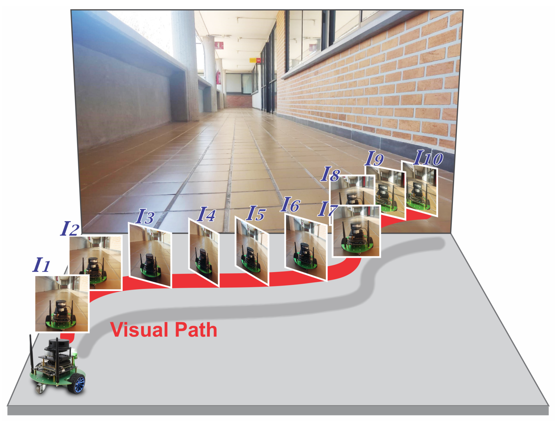
After completing the human-guided navigation to capture images of each environment, we proceeded to the learning stage for building the visual map. In this stage, we compare the visual map generation using hand-crafted feature extraction and matching using ORB and the deep learning approach within LoFTR. Since this first exploratory navigation and the learning stage were not performed simultaneously, the experiments were implemented in Python using Kornia [26], an Open Source Computer Vision Library for PyTorch, and executed in Google Colaboratory [27]. Geometric validation utilized the fundamental matrix with RANSAC and MAGSAC as feature-matching refinement (outlier detection). Moreover, we used different similarity threshold values from 0.1 to 0.9 to study the effect of the feature matching ratio between the last key image and a current frame. Thus, the lower the similarity, the fewer key images are selected; on the other hand, the higher the thresholds, the greater the number of key images.
We conducted extensive experiments using six datasets, combining ORB and LoFRT algorithms with varying similarity thresholds, for both ORB and LoFTR detectors. Table 3 presents the results for ORB with MAGSAC, specifically for dataset D1. It can be seen that for thresholds 0.1 to 0.5, the algorithm yields 1303 key images, that is, 33% of the total images, with similar average match values. For the threshold of 0.9, there are more key images, maintaining 66% of the images; hence, there are more matched points (an average of 244), as expected. The maximum quality was obtained with a threshold of 0.8; thus, 1434 key images were selected, which is 39% of the images. A mean of 43 matches was computed between consecutive key images.
We evaluated the ORB and LoFTR descriptors. 
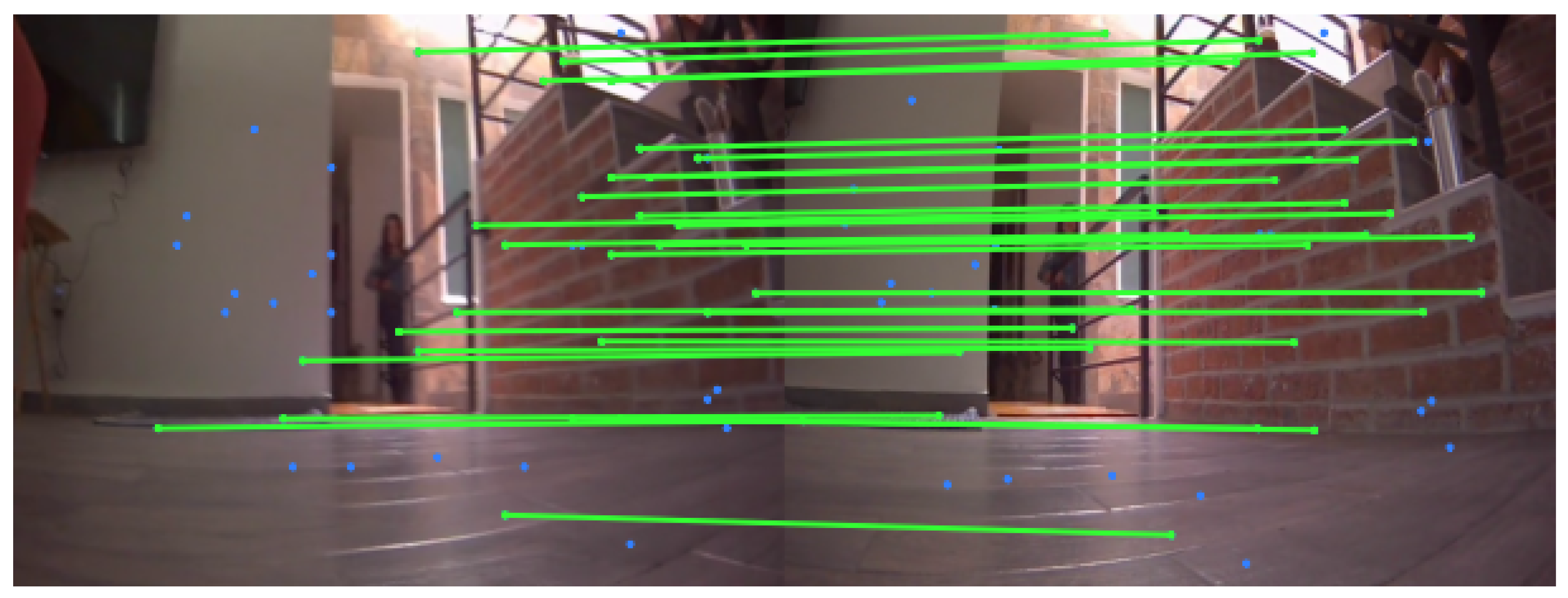
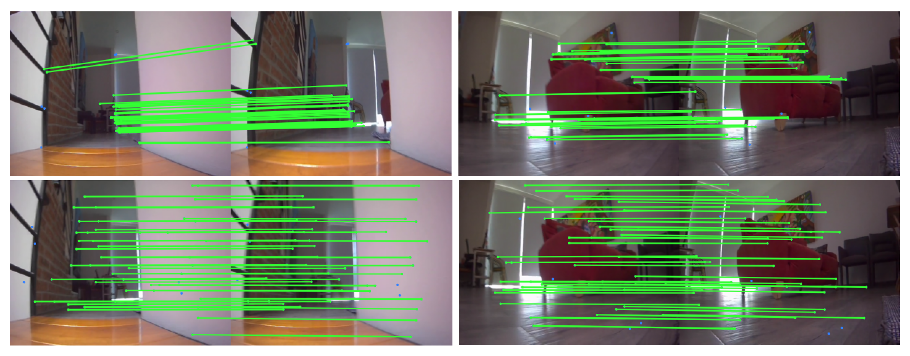
Figure 7 illustrates examples of only 50 matches between consecutive key images for the best quality visual map. The LoFTR+MAGSAC has more and better-distributed points than ORB+MAGSAC.
Table 4 exhibits the experiment conducted using LoFTR and MAGSAC for dataset D1. This table shows a better distribution of the key images selected by the algorithm. Specifically, at a threshold of 0.7, the algorithm identifies the best-quality visual map, with 269 key images, that is, 7% of the total images. This threshold gives a mean of matched points of 2180 instead of 19 achieved with ORB. Thus, a reliable fundamental matrix can be estimated.
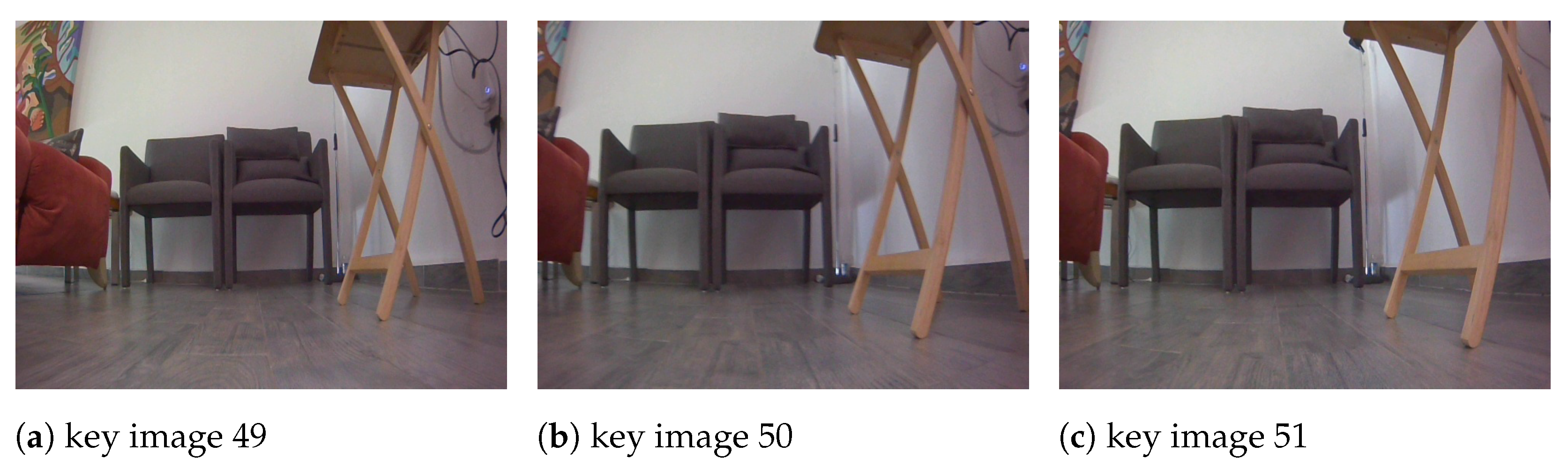
Figure 8 shows three consecutive key images obtained with LoFTR+MAGSAC.
Now, we evaluate our framework using the RANSAC algorithm as an outlier detector. Table 5 presents the results of ORB with RANSAC for Dataset D1. This combination yielded the best quality at the threshold of 0.7, where 1533 key images were obtained. The execution time of the algorithms was faster with MAGSAC.
Executing the algorithms using Jetbot’s GPU and RAM yields similar results. Tests were conducted within a virtual environment using Python 3.10, along with Jupyter Notebook. Dataset D1 was employed to obtain the average execution time per video frame. To keep the Google Colaboraty time factors consistent, we kept the original Notebook in the web server and established a local runtime WebSocket connection to use the available resources of the robot. An average time of 1.62 min per frame was obtained for MAGSAC, with a slightly slower time of 1.72 min per frame for RANSAC.On the other hand, executing our algorithm in the Cloud GPU resulted in an average time of 1.4 s per frame for the LoFTR and 0.05 s for ORB. Thus, all experiments were conducted in the offline mode.
Table 6 shows the results of LoFTR with RANSAC, which select more key images than LoFTR with MAGSAC. For instance, the optimal threshold is 0.5, at which we retrieved 152 key images; thus, 4% of the images were selected against the 7% selected with MAGSAC. Additionally, the mean matches were reduced with RANSAC, with 1356 vs. 2180 with the MAGSAC configuration.
It is worth noting that MAGSAC is more restrictive than RANSAC with higher thresholds, making it more convenient to create a visual map, in which fewer key images are selected but with higher similarity ratios. Based on these results, MAGSAC was chosen for subsequent experiments.
In the case of Dataset D2, Table 7 and Table 8 show the comparative study between ORB and LoFTR, respectively. With the ORB+MAGSAC combination, the number of key images remains constant at 454 for similarity thresholds ranging from 0.1 to 0.7. The average number of matches is around 20. The best memory quality, with a score of 0.86, was achieved using a threshold of 0.9. In this case, the memory map comprises 796 key images with a mean of 441 matches. When using LoFTR+MAGSAC, the number of key images increases as the threshold value grows. For instance, for the threshold of 0.6 that maximizes the quality, 45 key images were selected with 1122 mean matches, three times more matches than the best mean matches obtained with ORB. This corresponds to approximately only 1.2% of the total images comprising the visual map.
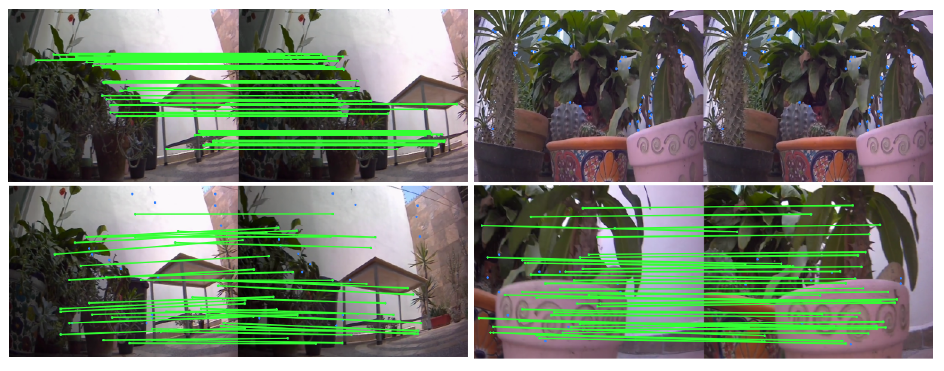
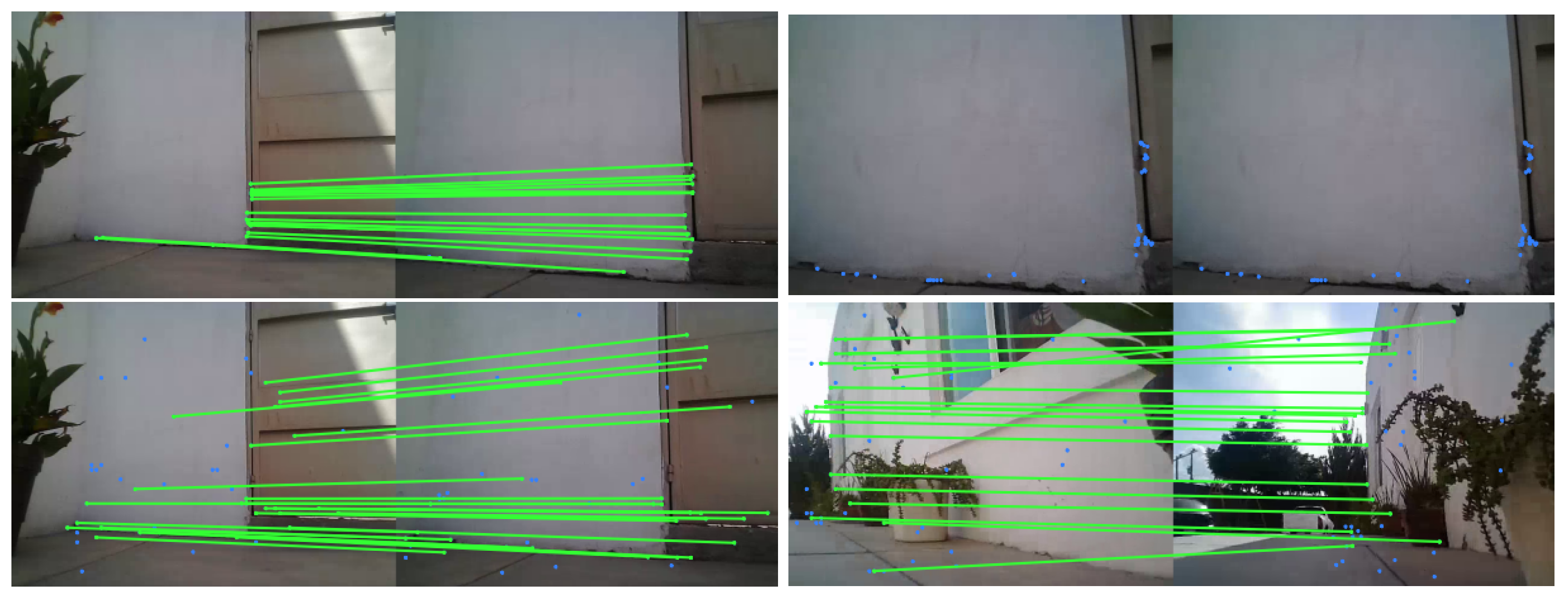
Figure 9 displays four examples of the first 50 matched points in consecutive key images employing the best visual map obtained with LoFTR+MAGSAC, and 
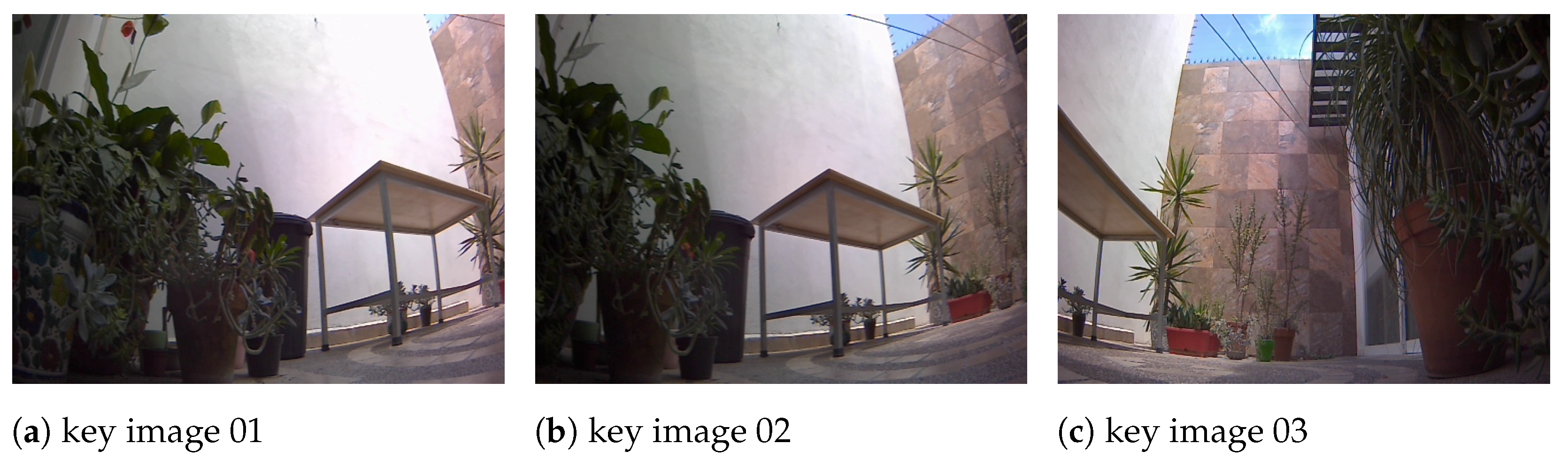
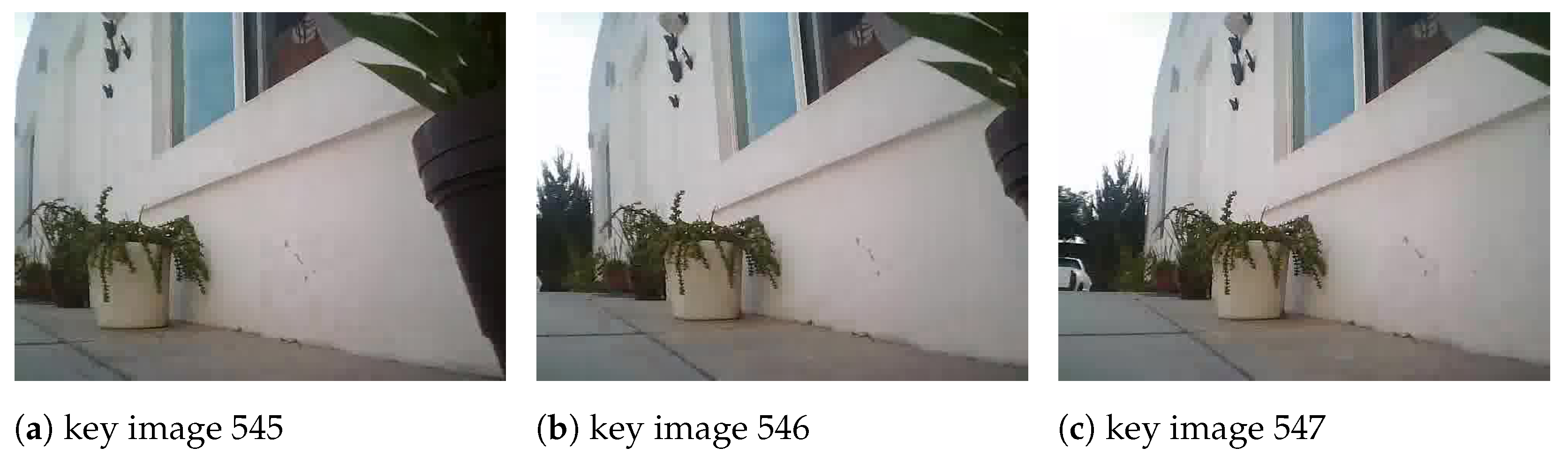
Figure 10 presents three examples of three consecutive key images from Dataset D2.
Evaluating our approach for Dataset D3, we observe a similar behavior to the previous datasets, where the ORB+MAGSAC was only available to match around 30 features. Meanwhile, the LoFTR+MAGSAC matches more than 500 features for threshold values higher than 0.5. This can be seen in Table 9 and Table 10, respectively. Additionally, the number of key images in the LoFTR+MAGSAC is lower than in the ORB+MAGSAC. Particularly, the best-quality memory of 0.53 for ORB+MAGSAC was obtained with a threshold of 0.9, obtaining 3000 key images. In total, 86% of the images were selected. On the other hand, LoFTR+MAGSAC with a similarity threshold of 0.2 obtained a quality of 0.77, around 49 mean matches, and only 32 key images (0.9% of the total images). 
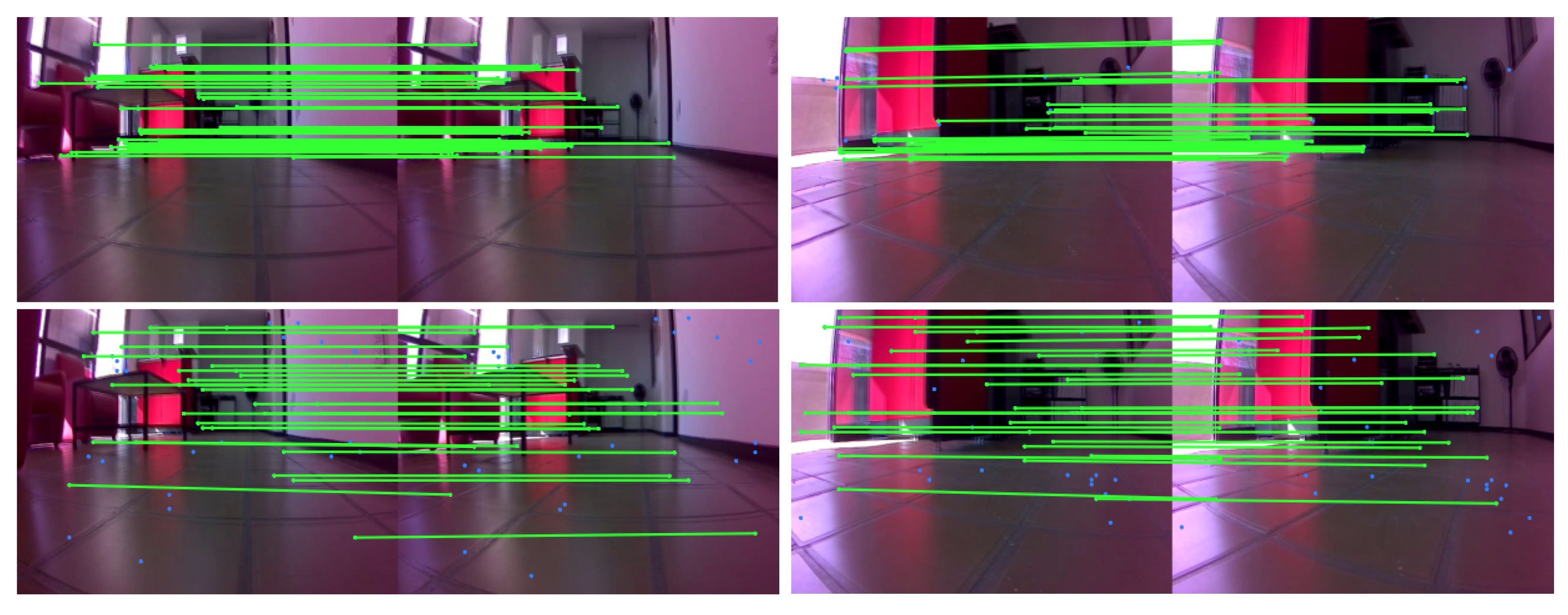
Figure 11 shows four examples of matched points in key images from the best-quality visual maps, and 
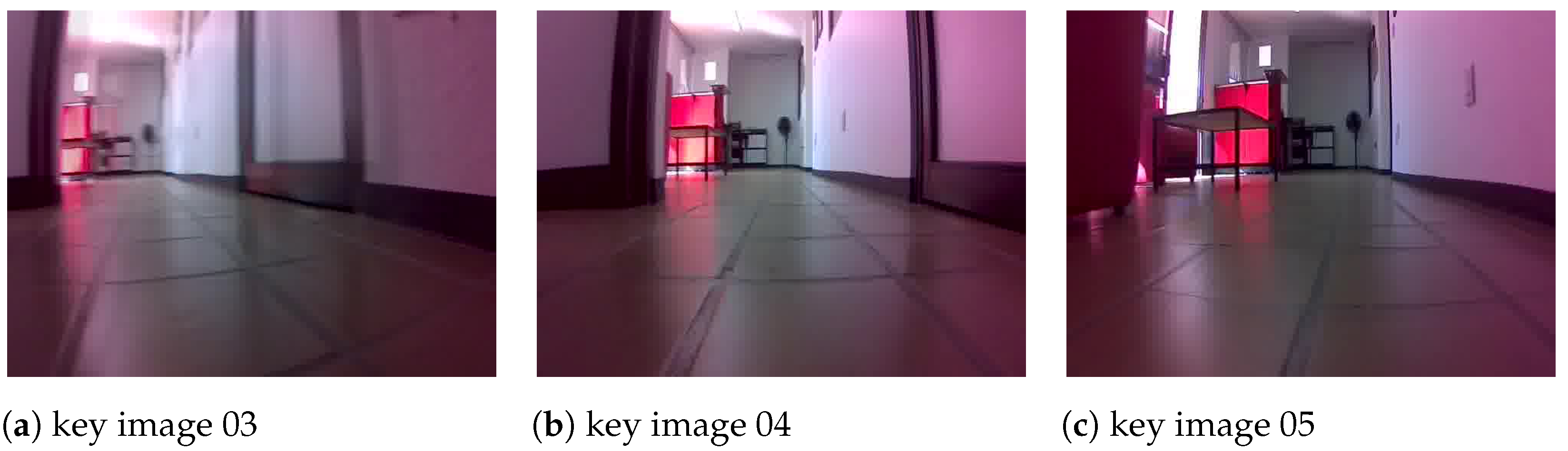
Figure 12 presents three examples of consecutive key images from the D3 dataset.
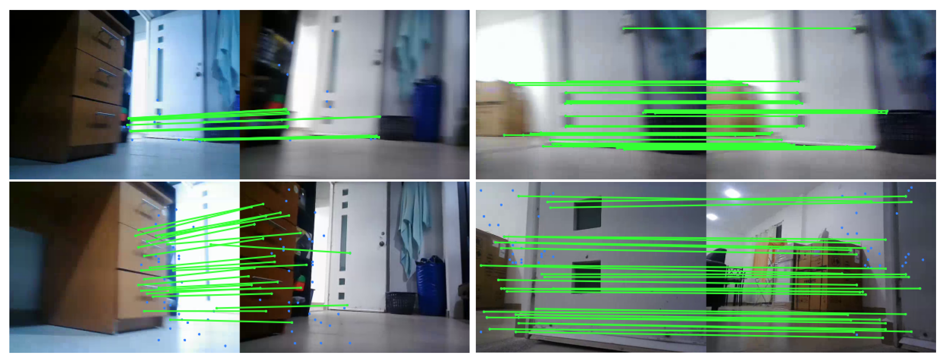
Table 11 shows the experiment results with LoFTR and MAGSAC with Dataset D4. This table shows a better distribution of the key images selected by the algorithm. At the threshold of 0.5, the best quality was obtained; it returned 63 key images. This threshold gives a mean of matched points of 1030 compared to ORB, whose mean of matched points is 28 with a threshold range of 0.1 to 0.5. At these thresholds, the number of key images was 2372, that is, 37 times more key images than LoFTR (see Table 12).
Figure 13 shows examples of matches between consecutive key images for the best threshold for both detectors. Additionally, 
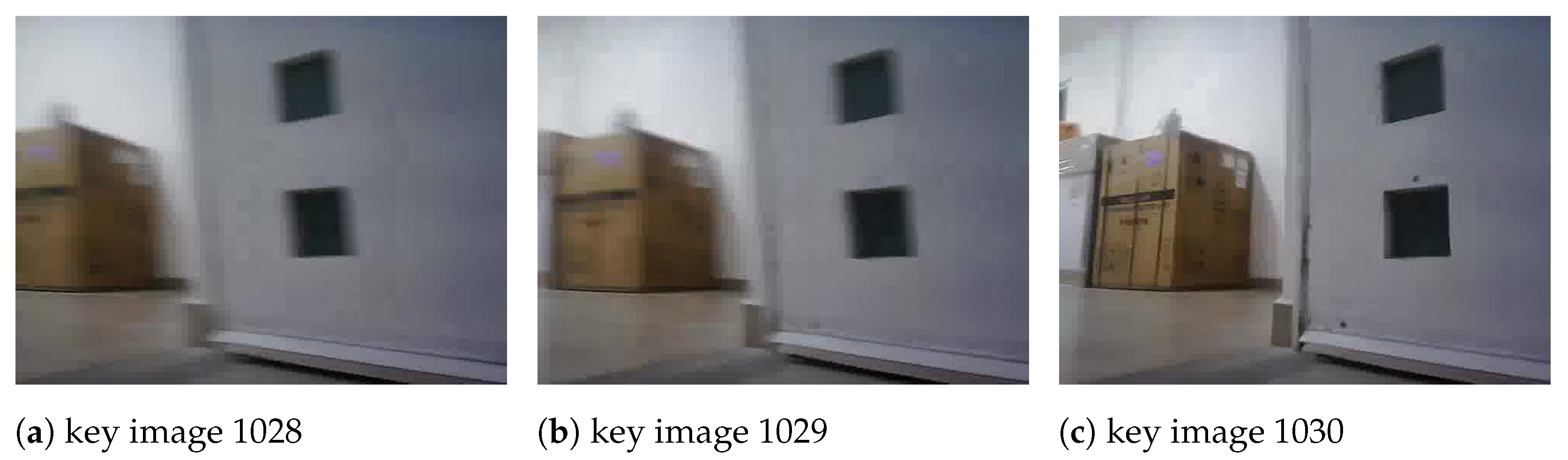
Figure 14 shows three consecutive key images obtained with LoFTR+MAGSAC.
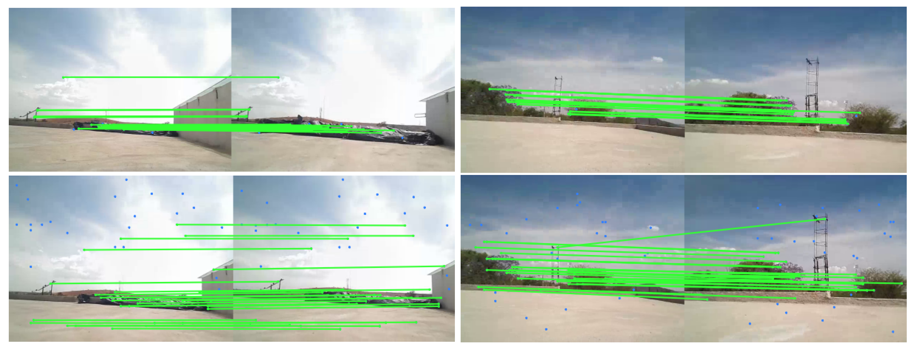
Table 13 shows the experiment results with LoFTR and MAGSAC with Dataset D5. A top quality of 0.77 was obtained with the 0.5 threshold value, selecting 54 key images with a mean matches of 640. The number of key images represents the 1.6% of the total images. On the scheme that used ORB (see Table 14, the best achieved quality was 0.96 but with only 20 matches in the 39 key images selected.
Figure 15 shows some images with the matches between consecutive key images for the optimal threshold of 0.7 and 0.5 for ORB and LoFTR, respectively. Additionally, 
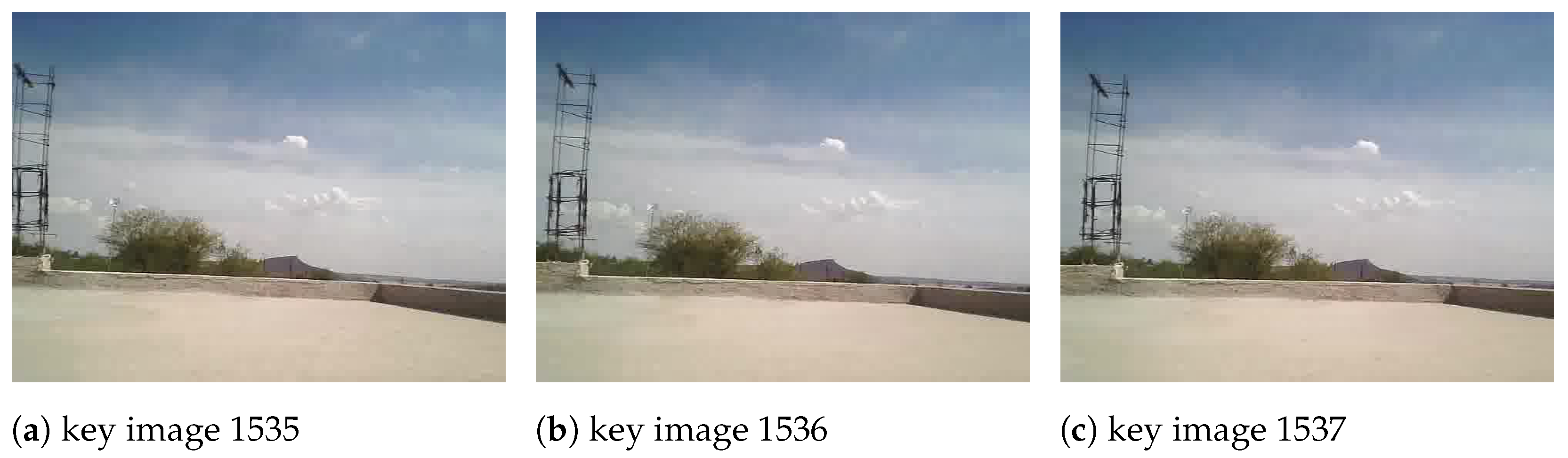
Figure 16 depicts three successive key images obtained with LoFTR+MAGSAC.
Table 15 shows the experiment results with LoFTR and MAGSAC with Dataset D6. In particular, using a threshold of 0.4, it achieved the best memory quality (0.75) and returned 32 key images, a mean of matched points of 319. For ORB, in comparison, whose results can be seen in Table 16, the optimal threshold of 0.7 obtained a mean of matched points of 18 and 3023 key images from 3330. Only seven images were discarded.
Figure 17 shows the images with the matches between consecutive key images for the best ORB and LoFTR detectors. Figure 18 presents an example of three key images obtained with LoFTR+MAGSAC.

4.4. Discussion

First, an ablation study was presented in the indoor Dataset D1 to select the best outlier algorithm between RANSAC and MAGSAC. We observed that MAGSAC was more restrictive with higher similarity thresholds, allowing us to create the visual map with fewer key images and higher similarity ratios. In general, with the datasets presented for indoor environments (D1, D3, and D4) and outdoor environments (D2, D5, and D6), we present extensive visual memory comparisons for ORB+MAGSAC and LoFTR+MAGSAC. The LoFTR+MAGSAC scheme presents the best results for the visual map quality. Additionally, LoFTR+MAGSAC reached the visual memory aim to obtain fewer key images with more matches between consecutive key images.
The LoFTR descriptors perform better under various conditions, such as lighting changes, viewpoint changes, and weather conditions. ORB uses variants of FAST as a detector, i.e., they detect key points by comparing gray levels along a circle of radius 3 to the gray level of the circle center. ORB uses oriented FAST key points, an improved version of FAST, including an adequate orientation component. The ORB descriptor is a binary vector of user-choice length. Each bit results from an intensity comparison between some pixels within a patch around the detected key points. The patches are previously smoothed with a Gaussian kernel to reduce noise. ORB computes a dominant orientation between the center of the key point and the intensity centroid of its patch to be robust to orientation changes. The key points are not robust to lighting changes present in the outdoor scenarios. On the other hand, LoFTR was trained with a large dataset, including images under different lighting conditions, view changes, stopovers, and hours of the day. For such a reason, LoFTR is more robust than ORB in these scenarios.
It is possible to extend the framework to any type of robot, for this is necessary to adapt the design of movement controllers to move the robot from an initial configuration to the final configuration keeping the key points on the images of the visual map. According to the kinematics model of the robot and the controller design, it is necessary to change the camera position on different parts of the robot to maintain specific parts of the environment in the camera field of view (fov) or avoid singularities with the controller. We planned to use an MPC; with this scheme, the camera location is not relevant. Using other sensors can help to deal with obstacles that lie out of the fov or the visual map generated and problems related to circumstances of the environment, such as the lighting or reflective or transparent surfaces.

5. Conclusions

We proposed a novel framework for generating a visual map to both indoor and outdoor environments. Our approach involves selecting key images sharing visual information between consecutive key images. Moreover, we introduced a quality measure to identify the optimal similarity threshold. This will allow visual localization and model predictive control for the localization and autonomous navigation stages. We employed a pre-trained LoFTR, constrained with a fundamental matrix between two consecutive key images; also, the MAGSAC algorithm effectively detects outliers during fundamental matrix estimation, improving the key image selection. Our proposed approach outperforms traditional hand-crafted methods, demonstrating the effectiveness of our visual map generation process, minimizing the number of key images selected, maximizing the memory quality, and ensuring that key images share enough visual information between them. For instance, from the ORB+MAGSAC approach, more than 30% of the images were selected as key images, with qualities around 0.5 to 0.7 with fewer than 100 mean matching features. For the LoFTR+MAGSAC, we obtained more than 1000 mean matching features and qualities greater than 0.7. Additionally, the key images only represent, at most, 8% of the total images. This improvement was also noticeable not only in indoor but also in outdoor environments, where ORB+MAGSAC obtained more key images and fewer matching features than LoFTR+MAGSAC.
Future work will include the evaluation of other deep learning-based approaches and the implementation of more efficient models in order to perform simultaneous localization and mapping in the onboard Jetson Nano of the Jetbot.

Author Contributions

Conceptualization, E.O.-M. and N.G.A.-M.; methodology, E.O.-M.; software, E.O.-M., C.A.G.-P., E.M. and N.G.A.-M.; validation, E.M., C.A.G.-P. and N.G.A.-M.; investigation, E.O.-M., C.A.G.-P., E.M. and N.G.A.-M.; resources, E.O.-M., C.A.G.-P., E.M. and N.G.A.-M.; writing—original draft preparation, E.O.-M., C.A.G.-P., E.M. and N.G.A.-M.; visualization, C.A.G.-P., E.M. and N.G.A.-M.; supervision, N.G.A.-M.; funding acquisition, E.O.-M., E.M. and N.G.A.-M. All authors have read and agreed to the published version of the manuscript.

Funding

This work was supported in part by Universidad Iberoamericana León, Tecnológico Nacional de México/ITS de Guanajuato (Instituto Tecnológico Superior de Guanajuato), and by the University of Guanajuato Grant NUA 147347. Partially by the Mexican Council of Science and Technology CONACyT Grant no. 626154/755609.

Institutional Review Board Statement

Not applicable.

Informed Consent Statement

Not applicable.

Data Availability Statement

Data available under formal demand.

Conflicts of Interest

The authors declare no conflict of interest.

Abbreviations

The following abbreviations are used in this manuscript:
AIArtificial Intelligence
BRIEFBinary Robust Independent Elementary Features
FASTFeatures from Accelerated Segment Test
FPSFrames per Second
LOFTRDetector-Free Local Feature Matching with Transformers
MAGSACMarginalizing Sample Consensus
MNNMutual Nearest Neighbor
MPCModel Predictive Control
ORBOriented FAST and rotated BRIEF
RANSACRandom Sample Consensus
ROSRobot Operating System

References

  1. Siegwart, R.; Nourbakhsh, I.R.; Scaramuzza, D. Introduction to Autonomous Mobile Robots; MIT Press: Cambridge, MA, USA, 2011. [Google Scholar]
  2. Courbon, J.; Mezouar, Y.; Martinet, P. Autonomous Navigation of Vehicles from a Visual Memory Using a Generic Camera Model. IEEE Trans. Intell. Transp. Syst. 2009, 10, 392–402. [Google Scholar] [CrossRef]
  3. Aldana-Murillo, N.G.; Sandoval, L.; Hayet, J.B.; Esteves, C.; Becerra, H.M. Coupling humanoid walking pattern generation and visual constraint feedback for pose-regulation and visual path-following. Robot. Auton. Syst. 2020, 128, 103497. [Google Scholar] [CrossRef]
  4. Aldana-Murillo, N.G.; Hayet, J.B.; Becerra, H.M. Evaluation of Local Descriptors for Vision-Based Localization of Humanoid Robots. In Proceedings of the Pattern Recognition, Mexico City, Mexico, 24–27 June 2015; Springer International Publishing: Berlin/Heidelberg, Germany, 2015; pp. 179–189. [Google Scholar]
  5. Aldana-Murillo, N.G.; Hayet, J.B.; Becerra, H.M. Comparison of Local Descriptors for Humanoid Robots Localization Using a Visual Bag of Words Approach. Intell. Autom. Soft Comput. 2018, 24, 471–481. [Google Scholar] [CrossRef]
  6. Delfin, J.; Becerra, H.M.; Arechavaleta, G. Humanoid navigation using a visual memory with obstacle avoidance. Robot. Auton. Syst. 2018, 109, 109–124. [Google Scholar] [CrossRef]
  7. Ovalle-Magallanes, E.; Aldana-Murillo, N.G.; Avina-Cervantes, J.G.; Ruiz-Pinales, J.; Cepeda-Negrete, J.; Ledesma, S. Transfer Learning for Humanoid Robot Appearance-Based Localization in a Visual Map. IEEE Access 2021, 9, 6868–6877. [Google Scholar] [CrossRef]
  8. Diosi, A.; Segvic, S.; Remazeilles, A.; Chaumette, F. Experimental Evaluation of Autonomous Driving Based on Visual Memory and Image-Based Visual Servoing. IEEE Trans. Intell. Transp. Syst. 2011, 12, 870–883. [Google Scholar] [CrossRef] [Green Version]
  9. López-Martínez, A.; Cuevas, F.; Sosa-Balderas, J. Visual Memory Construction for Autonomous Humanoid Robot Navigation. In Progress in Optomechatronic Technologies: Proceedings of International Symposium on Optomechatronic (2018); Springer: Berlin/Heidelberg, Germany, 2019; pp. 103–109. [Google Scholar]
  10. Huang, C.; Mees, O.; Zeng, A.; Burgard, W. Visual Language Maps for Robot Navigation. arXiv 2022, arXiv:2210.05714. [Google Scholar]
  11. Li, D.; Zhang, Q.; Zhao, D. Graph attention memory for visual navigation. In Proceedings of the 2022 4th International Conference on Data-driven Optimization of Complex Systems (DOCS), Chengdu, China, 28–30 October 2022; pp. 1–7. [Google Scholar]
  12. Crespo, J.; Castillo, J.C.; Mozos, O.M.; Barber, R. Semantic information for robot navigation: A survey. Appl. Sci. 2020, 10, 497. [Google Scholar] [CrossRef] [Green Version]
  13. Papapetros, I.T.; Balaska, V.; Gasteratos, A. Multi-layer map: Augmenting semantic visual memory. In Proceedings of the 2020 International Conference on Unmanned Aircraft Systems (ICUAS), Athens, Greece, 1–4 September 2020; pp. 1206–1212. [Google Scholar]
  14. Ma, J.; Jiang, X.; Fan, A.; Jiang, J.; Yan, J. Image matching from handcrafted to deep features: A survey. Int. J. Comput. Vis. 2021, 129, 23–79. [Google Scholar] [CrossRef]
  15. Tian, L. Matching Images from Different Viewpoints with Deep Learning Based on LoFTR and MAGSAC++. In Proceedings of the 2023 5th International Conference on Image Processing and Machine Vision, New York, NY, USA, 13–15 January 2023; pp. 18–23. [Google Scholar]
  16. Hartley, R.; Zisserman, A. Multiple View Geometry in Computer Vision, 2nd ed.; Cambridge University Press: Cambridge, UK, 2006. [Google Scholar]
  17. Fischler, M.A.; Bolles, R.C. Random Sample Consensus: A Paradigm for Model Fitting with Applications to Image Analysis and Automated Cartography. Commun. ACM 1981, 24, 381–395. [Google Scholar] [CrossRef]
  18. Barath, D.; Matas, J.; Noskova, J. MAGSAC: Marginalizing Sample Consensus. In Proceedings of the IEEE/CVF Conference on Computer Vision and Pattern Recognition (CVPR), Long Beach, CA, USA, 15–20 June 2019. [Google Scholar]
  19. Rublee, E.; Rabaud, V.; Konolige, K.; Bradski, G. ORB: An efficient alternative to SIFT or SURF. In Proceedings of the IEEE International Conference on Computer Vision, Barcelona, Spain, 6–13 November 2011; pp. 2564–2571. [Google Scholar]
  20. Sun, J.; Shen, Z.; Wang, Y.; Bao, H.; Zhou, X. LoFTR: Detector-free local feature matching with transformers. In Proceedings of the IEEE/CVF Conference on Computer Vision and Pattern Recognition, Nashville, TN, USA, 15–20 June 2021; pp. 8922–8931. [Google Scholar]
  21. Rosten, E.; Drummond, T. Machine learning for high-speed corner detection. In Proceedings of the European Conference on Computer Vision, Graz, Austria, 7–13 May 2006; pp. 430–443. [Google Scholar]
  22. Calonder, M.; Lepetit, V.; Strecha, C.; Fua, P. Brief: Binary robust independent elementary features. Eur. Conf. Comput. Vis. 2010, 778–792. [Google Scholar] [CrossRef]
  23. JetBot Ros Ai Kit. Available online: https://www.waveshare.com/wiki/JetBot_ROS_AI_Kit (accessed on 10 April 2023).
  24. Quigley, M.; Conley, K.; Gerkey, B.P.; Faust, J.; Foote, T.; Leibs, J.; Wheeler, R.; Ng, A.Y. Robotic Operating System. Available online: https://www.ros.org/ (accessed on 10 April 2023).
  25. Bradski, G. The OpenCV Library. Dr. Dobb’s J. Softw. Tools 2000. Available online: http://opencv.org/ (accessed on 10 April 2023).
  26. Riba, E.; Mishkin, D.; PONSA, D.; Rublee, E.; Bradski, G. Kornia: An Open Source Differentiable Computer Vision Library for PyTorch. In Proceedings of the Winter Conference on Applications of Computer Vision, Snowmass Village, CO, USA, 1–5 March 2020. [Google Scholar]
  27. Bisong, E. Google Colaboratory. In Building Machine Learning and Deep Learning Models on Google Cloud Platform: A Comprehensive Guide for Beginners; Apress: Berkeley, CA, USA, 2019; pp. 59–64. [Google Scholar]
Figure 1. The visual map M comprises a set of key images that model an environment where the robot can be localized and navigated.
Eng 04 00092 g001
Figure 2. The fundamental matrix: two-view geometry in the case of non-planar scenes. An X point in 3D is shown in two images, x 1 in the first and x 2 in the second. The camera centers ( C 1 and C 2 ), the point X , and its projections x 1 and x 2 lie in a common plane π . e 1 and e 2 are the epipolar points. The epipole is the point of intersection of the line joining the camera centers with the image plane. The fundamental matrix is the algebraic representation of epipolar geometry.
Eng 04 00092 g002
Figure 3. Image matching general pipeline. Both hand-crafted and deep learning-based approaches use feature detection, description, matching, and geometry verification.
Eng 04 00092 g003
Figure 4. Matching process between two consecutive key images. The matches that meet the fundamental matrix constraint are shown in green lines and in blue points otherwise.
Eng 04 00092 g004
Figure 5. Relevant JetBot components.
Eng 04 00092 g005
Figure 6. Samples of images taken from the robot camera for each dataset.
Eng 04 00092 g006
Figure 7. Examples of matched points between key images for Dataset D1. (Top row): ORB+MAGSAC. (Bottom row): LoFTR+MAGSAC.
Eng 04 00092 g007
Figure 8. Examples of key images obtained with LoFTR+MAGSAC for Dataset D1.
Eng 04 00092 g008
Figure 9. Examples of matched points between key images for Dataset D2. (Top row): ORB+MAGSAC. (Bottom row): LoFTR+MAGSAC.
Eng 04 00092 g009
Figure 10. Examples of key images obtained with LoFTR+MAGSAC for Dataset D2.
Eng 04 00092 g010
Figure 11. Examples of matched points between key images for Dataset D1. (Top row): ORB+MAGSAC. (Bottom row): LoFTR+MAGSAC.
Eng 04 00092 g011
Figure 12. Examples of key images obtained with LoFTR+MAGSAC for Dataset D3.
Eng 04 00092 g012
Figure 13. Examples of matched points between key images for Dataset D4. (Top row): ORB+MAGSAC. (Bottom row): LoFTR+MAGSAC.
Eng 04 00092 g013
Figure 14. Examples of key images obtained with LoFTR+MAGSAC for Dataset D4.
Eng 04 00092 g014
Figure 15. Examples of matched points between key images for Dataset D5. (Top row): ORB+MAGSAC. (Bottom row): LoFTR+MAGSAC.
Eng 04 00092 g015
Figure 16. Examples of key images obtained with LoFTR+MAGSAC for Dataset D5.
Eng 04 00092 g016
Figure 17. Examples of matched points between key images for Dataset D6. (Top row): ORB+MAGSAC. (Bottom row): LoFTR+MAGSAC.
Eng 04 00092 g017
Figure 18. Examples of key images obtained with LoFTR+MAGSAC for Dataset D6.
Eng 04 00092 g018
Table 1. JetBot professional ROS AI Kit characteristics.
Software DevKitLinux DistributionROS DistributionMicrocontroller
Jetpack 4.5Ubuntu 18.04Melodic Morenia [24]Raspberry Pi RP2040
Table 2. Datasets used for the visual map generation.
DatasetEnvironmentNumber of FramesImage Size (px × px)Description
D1Indoor3703 640 × 480 Room
D2Outdoor3525 640 × 480 Backyard
D3Indoor3477 640 × 480 Corridor
D4Indoor3004 640 × 480 Traveling between two rooms
D5Outdoor3238 640 × 480 Roof
D6Outdoor3330 640 × 480 Courtyard
Table 3. Visual map generation with ORB+MAGSAC for Dataset D1.
ThresholdNumber of Key ImagesMin. MatchesMax. MatchesMean MatchesQuality
0.11303145629.80.71
0.21303145629.80.71
0.31303145629.80.71
0.41303145629.80.71
0.51303145629.80.71
0.61305147929.90.71
0.713221431419.80.70
0.814341457643.00.74
0.9250517501244.80.62
Table 4. Visual map generation with LoFTR+MAGSAC for Dataset D1.
ThresholdNumber of Key ImagesMin. MatchesMax. MatchesMean MatchesQuality
0.115113417.70.77
0.2151212240.00.71
0.32211450178.10.69
0.43390886446.40.71
0.5602471413892.80.76
0.612246024911551.70.81
0.726997929422180.90.84
0.821771535871493.10.63
0.93566297040413416.30.48
Table 5. Visual map generation with ORB+RANSAC for Dataset D1.
ThresholdNumber of Key ImagesMin. MatchesMax. MatchesMean MatchesQuality
0.11303124929.70.71
0.21303124929.70.71
0.31303124929.70.71
0.41303124929.70.71
0.51303124929.70.71
0.613301221418.00.70
0.715331438338.20.73
0.8278114507204.60.53
0.9359839607359.60.47
Table 6. Visual map generation with LoFTR+RANSAC for Dataset D1.
ThresholdNumber of Key ImagesMin. MatchesMax. MatchesMean MatchesQuality
0.115102716.00.74
0.22111344118.40.65
0.343153662428.70.65
0.4773031274863.30.70
0.515280318431356.20.75
0.69951229882030.60.69
0.721921235521597.70.57
0.835972433272447.80.46
0.93625337738233822.90.48
Table 7. Visual map generation with ORB+MAGSAC for Dataset D2.
ThresholdNumber of Key ImagesMin. MatchesMax. MatchesMean MatchesQuality
0.1454124221.70.85
0.2454124221.70.85
0.3454124221.70.85
0.4454124221.70.85
0.5454124221.70.85
0.6454124221.70.85
0.7468136522.70.84
0.86241640775.60.84
0.979617950441.60.86
Table 8. Visual map generation with LoFTR+MAGSAC for Dataset D2.
ThresholdNumber of Key ImagesMin. MatchesMax. MatchesMean MatchesQuality
0.110264437.20.62
0.210264437.20.62
0.3133610366.20.67
0.41555458157.60.72
0.521164784396.90.77
0.64519918941122.30.82
0.760472825831771.00.77
0.8723131934142716.70.82
0.93236238236283240.00.52
Table 9. Visual map generation with ORB+MAGSAC for Dataset D3.
ThresholdNumber of Key ImagesMin. MatchesMax. MatchesMean MatchesQuality
0.128661312628.10.48
0.228661312628.10.48
0.328661312628.10.48
0.428661312628.10.48
0.528661312628.10.48
0.628661312628.10.48
0.7286515275102.70.49
0.828941531036.70.50
0.9300023469200.40.53
Table 10. Visual map generation with LoFTR+MAGSAC for Dataset D3.
ThresholdNumber of Key ImagesMin. MatchesMax. MatchesMean MatchesQuality
0.1311023149.10.76
0.2321023149.40.77
0.3509360122.90.71
0.410812894345.00.72
0.5386121953919.60.74
0.6955122491971.90.69
0.730061227711266.50.43
0.834231438571450.70.43
0.93465284028402840.00.47
Table 11. Visual map generation with LoFTR+MAGSAC for Dataset D4.
ThresholdNumber of Key ImagesMin. MatchesMax. MatchesMean MatchesQuality
0.111126527.00.73
0.212115730.50.70
0.31713545144.50.70
0.424163053502.00.74
0.5635919631030.00.78
0.63961430531443.00.76
0.719831237292860.10.60
0.828341539092655.30.45
0.92984337641753399.30.46
Table 12. Visual map generation with ORB+MAGSAC for Dataset D4.
ThresholdNumber of Key ImagesMin. MatchesMax. MatchesMean MatchesQuality
0.123721322828.20.56
0.223721322828.20.56
0.323721322828.20.56
0.423721322828.20.56
0.523721322828.20.56
0.623731322828.20.55
0.723781522824.60.49
0.823951625726.40.54
0.9246630600136.40.54
Table 13. Visual map generation with LoFTR+MAGSAC for Dataset D5.
ThresholdNumber of Key ImagesMin. MatchesMax. MatchesMean MatchesQuality
0.17243428.70.58
0.293712068.40.63
0.31259440151.70.70
0.420121556286.10.74
0.5541762002640.20.77
0.610832753020913.40.65
0.72987118232042095.40.40
0.83034230730122572.50.44
0.93039290135683567.60.49
Table 14. Visual map generation with ORB+MAGSAC for Dataset D5.
ThresholdNumber of Key ImagesMin. MatchesMax. MatchesMean MatchesQuality
0.139143920.90.96
0.239143920.90.96
0.339143920.90.96
0.439143920.90.96
0.539143920.90.96
0.639143920.90.96
0.739143920.90.96
0.8531519253.60.94
0.924616530185.80.93
Table 15. Visual map generation with LoFTR+MAGSAC for Dataset D6.
ThresholdNumber of Key ImagesMin. MatchesMax. MatchesMean MatchesQuality
0.14183123.30.57
0.2193918295.90.64
0.32765488174.70.69
0.4321351672319.90.75
0.5302352114421170.00.42
0.6236722429871628.30.52
0.73104104222742199.00.43
0.83145243224322432.00.48
0.93147272531882725.10.50
Table 16. Visual map generation with ORB+MAGSAC for Dataset D6.
ThresholdNumber of Key ImagesMin. MatchesMax. MatchesMean MatchesQuality
0.13023171818.00.55
0.23023171818.00.55
0.33023171818.00.55
0.43023171818.00.55
0.53023171818.00.55
0.63023171818.00.55
0.73023171818.00.55
0.83023161916.00.49
0.930371920129.40.50
Disclaimer/Publisher’s Note: The statements, opinions and data contained in all publications are solely those of the individual author(s) and contributor(s) and not of MDPI and/or the editor(s). MDPI and/or the editor(s) disclaim responsibility for any injury to people or property resulting from any ideas, methods, instructions or products referred to in the content.

