Author Contributions
Conceptualization, M.L., E.F. and G.G.; methodology, M.L., R.G.-M. and E.F.; software, M.L. and E.T.; validation, M.L., R.G.-M., I.P. and E.T., formal analysis, M.L. and E.F.; investigation, M.L., R.G.-M. and I.P.; writing—original draft preparation, M.L. and E.F.; writing—review and editing, M.L., R.G.-M., G.G. and E.F.; supervision, G.G. and E.F.; project administration, G.G. and E.F.; funding acquisition G.G. and E.F. All authors have read and agreed to the published version of the manuscript.
Figure 1.
One-line diagram of two three-phase inverters connected in parallel with LCL filters.
Figure 1.
One-line diagram of two three-phase inverters connected in parallel with LCL filters.
Figure 2.
Simplified scheme of two three-phase inverters connected in parallel.
Figure 2.
Simplified scheme of two three-phase inverters connected in parallel.
Figure 3.
VA1 and VA2 voltage variation according to: (a) current variation being > ; (b) inductance variation being La2 > La1.
Figure 3.
VA1 and VA2 voltage variation according to: (a) current variation being > ; (b) inductance variation being La2 > La1.
Figure 4.
Experimental setup.
Figure 4.
Experimental setup.
Figure 5.
Control structure.
Figure 5.
Control structure.
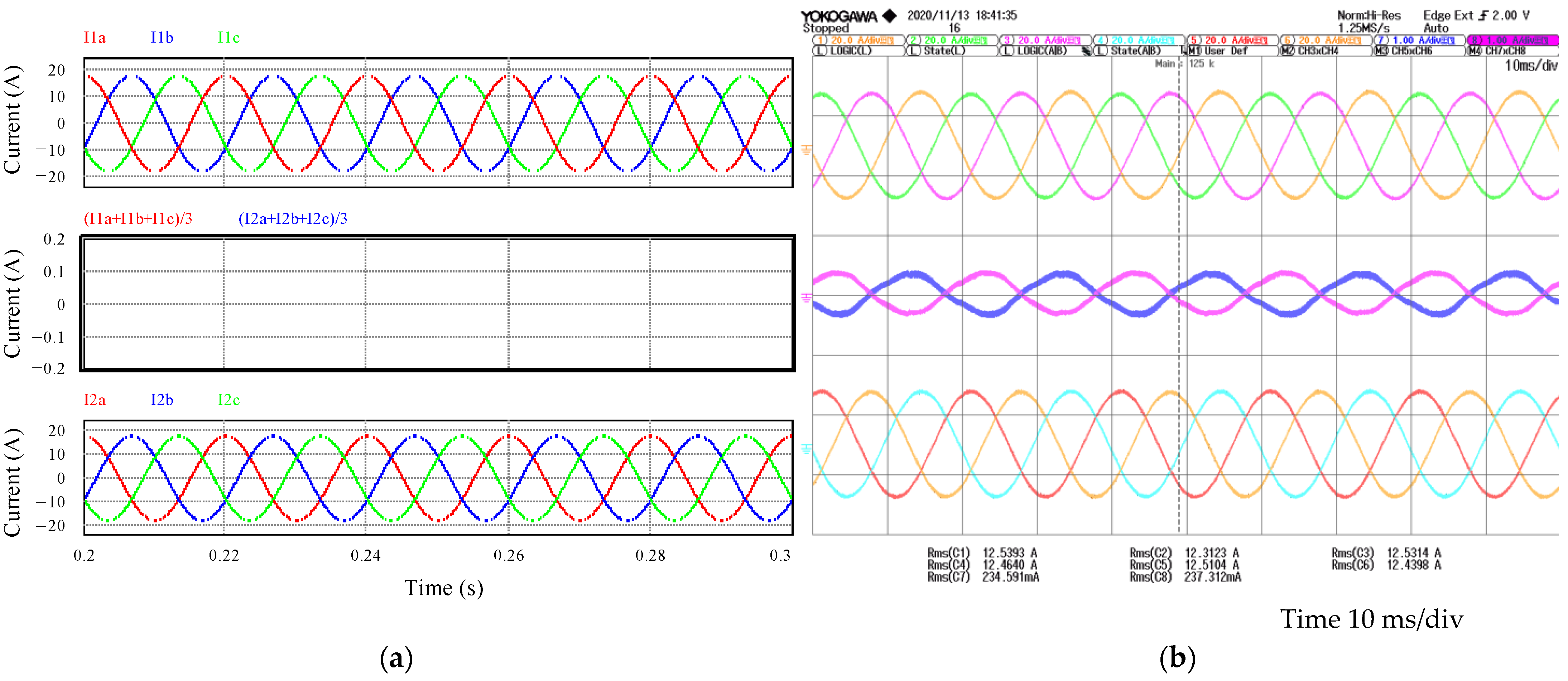
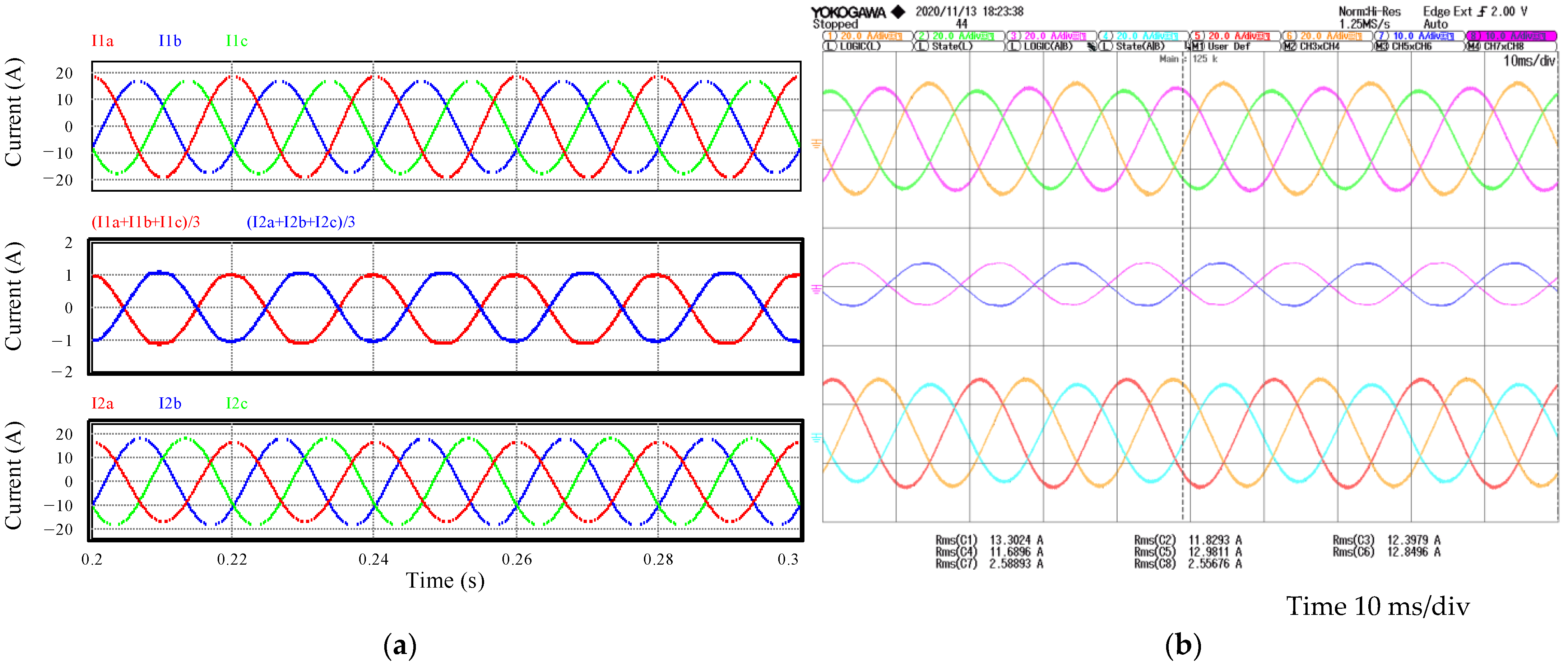
Figure 6.
Circulating current in a balanced system composed of two identical parallel inverters. Phase currents of inverter #1 at the top, circulating currents in the middle and phase currents of inverter #2 at the bottom. (a) 100% load factor simulation results; (b) 100% load factor experimental results.
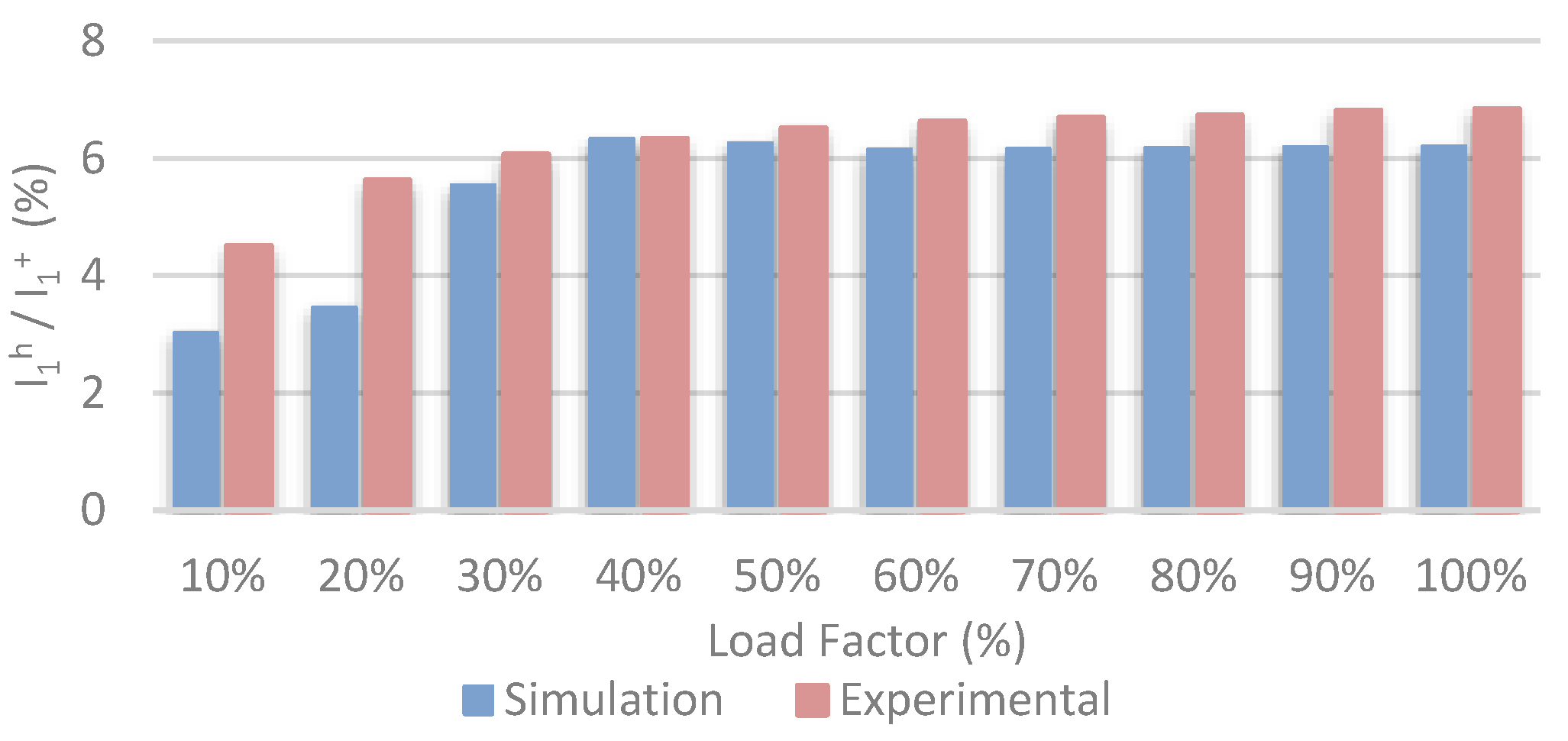
Figure 7.
Simulation and experimental harmonic of 50 Hz I1h/I1+ of the circulating current in the whole power range for a balanced system.
Figure 7.
Simulation and experimental harmonic of 50 Hz I1h/I1+ of the circulating current in the whole power range for a balanced system.
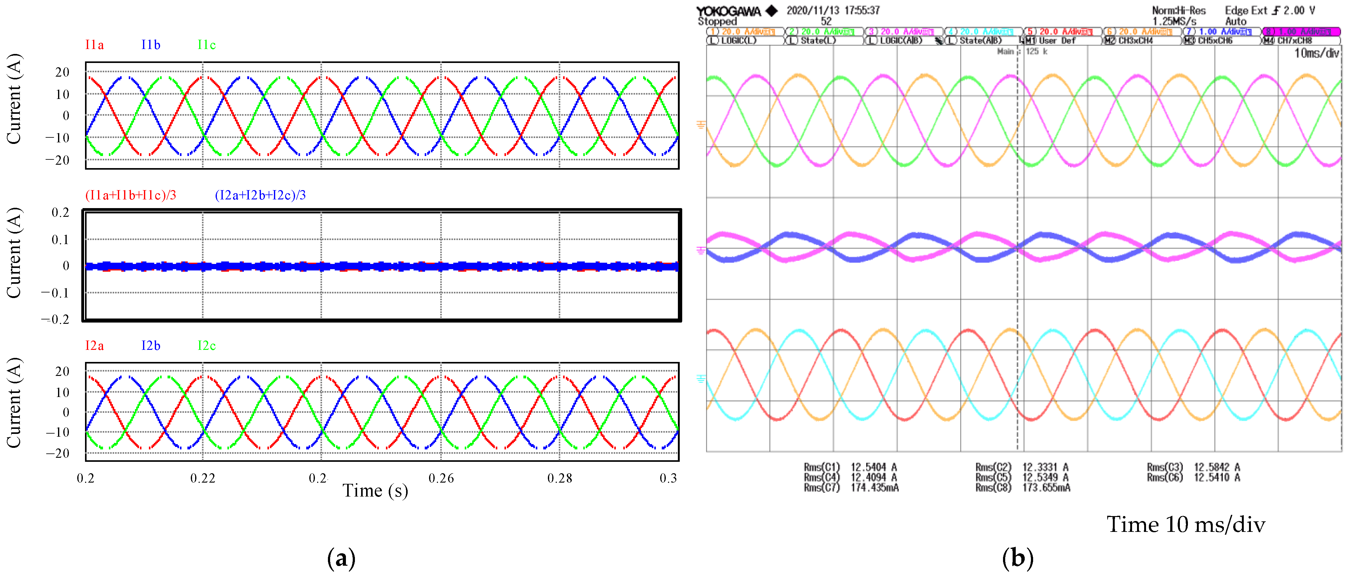
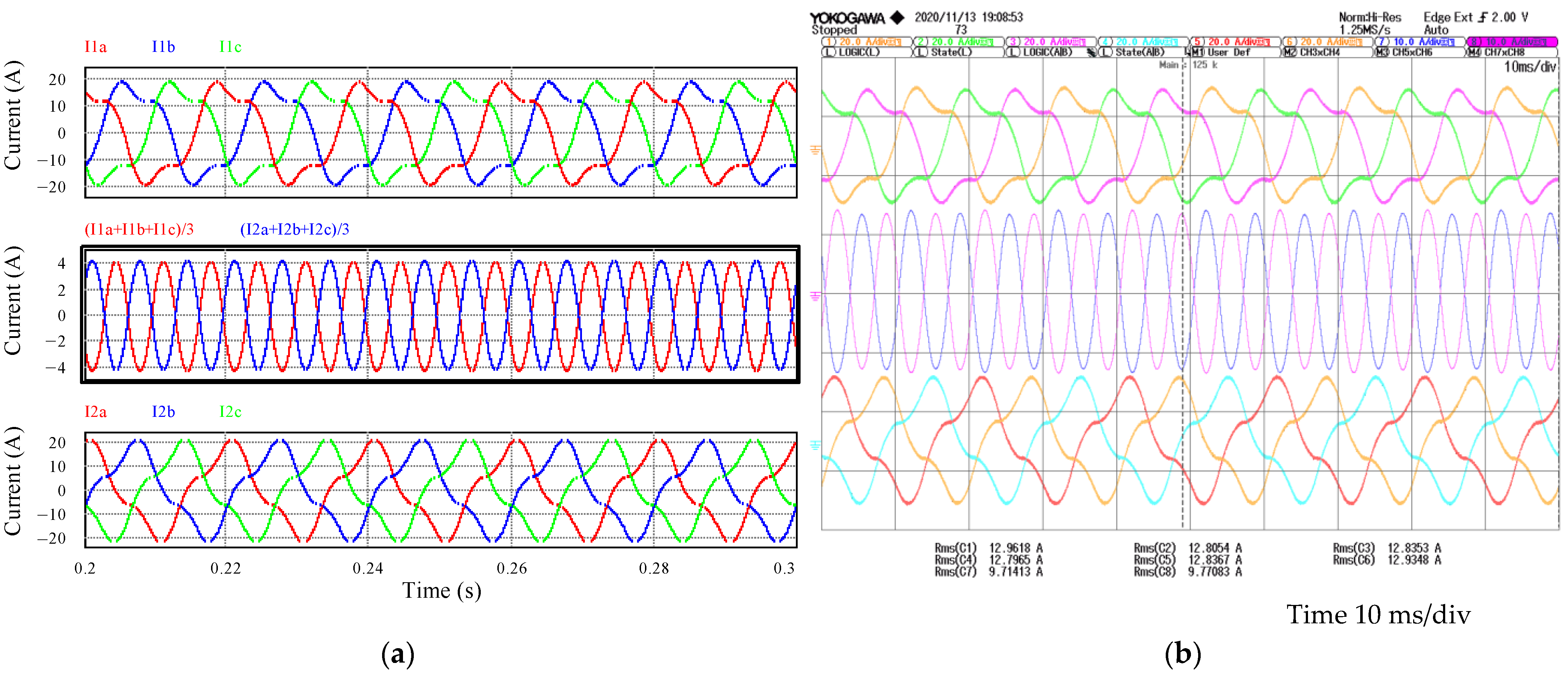
Figure 8.
Circulating current with unbalanced inductors between inverter #1 and #2 (La1 = 5 mH, and La2 = 7 mH). Phase currents of inverter #1 at the top, circulating currents in the middle, and phase currents of inverter #2 at the bottom (a) 100% load factor simulation results; (b) 100% load factor experimental results.
Figure 9.
Simulation and experimental harmonics of: (a) 50 Hz I1h/I1+; and (b) 150 Hz I3h/I1+ in the whole range of power of the circulating current with unbalanced inductors between inverter #1 and #2 (La1 = 5 mH and, La2 = 7 mH).
Figure 9.
Simulation and experimental harmonics of: (a) 50 Hz I1h/I1+; and (b) 150 Hz I3h/I1+ in the whole range of power of the circulating current with unbalanced inductors between inverter #1 and #2 (La1 = 5 mH and, La2 = 7 mH).
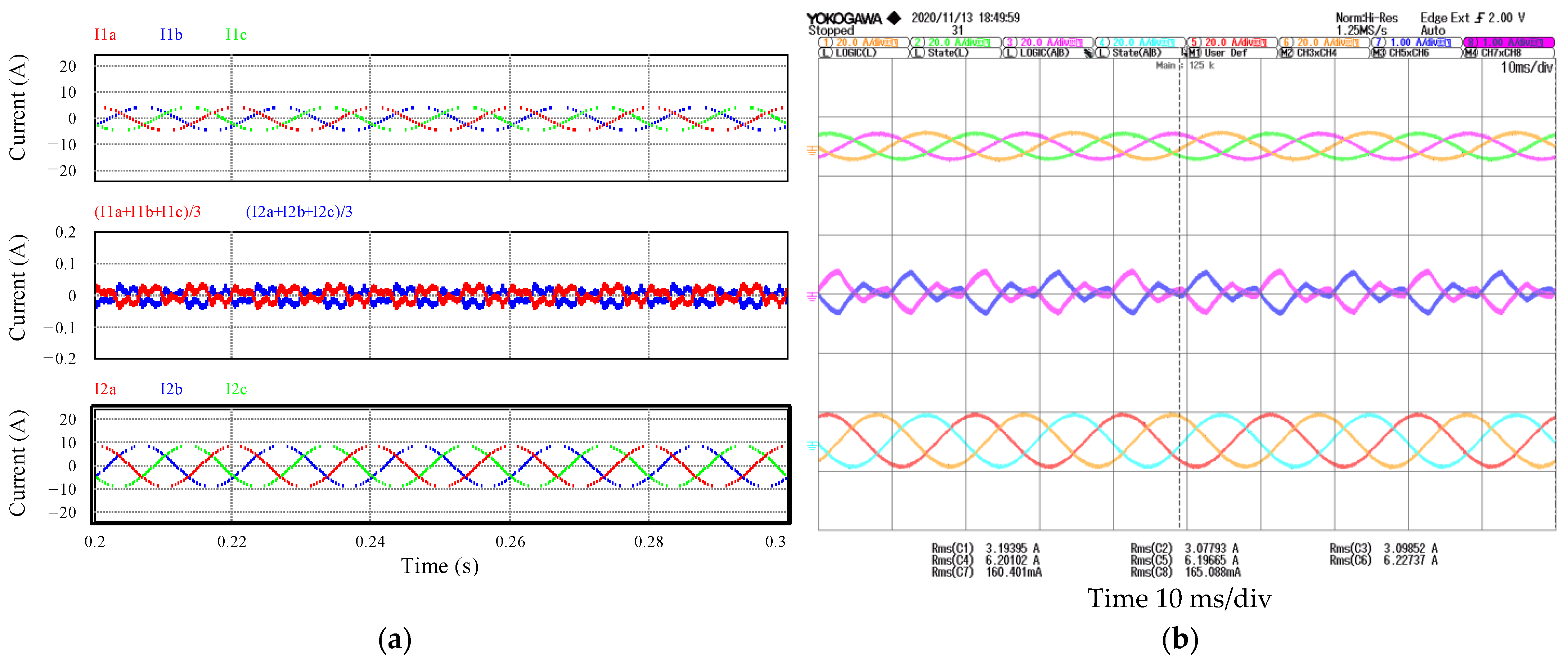
Figure 10.
(a) Simulation results with 25% load factor in inverter #1 and 50% in inverter #2; (b) experimental results with 25% load factor in inverter #1 and 50% in inverter #2. Phase currents of inverter #1 at the top, circulating currents in the middle, and phase currents of inverter #2 at the bottom.
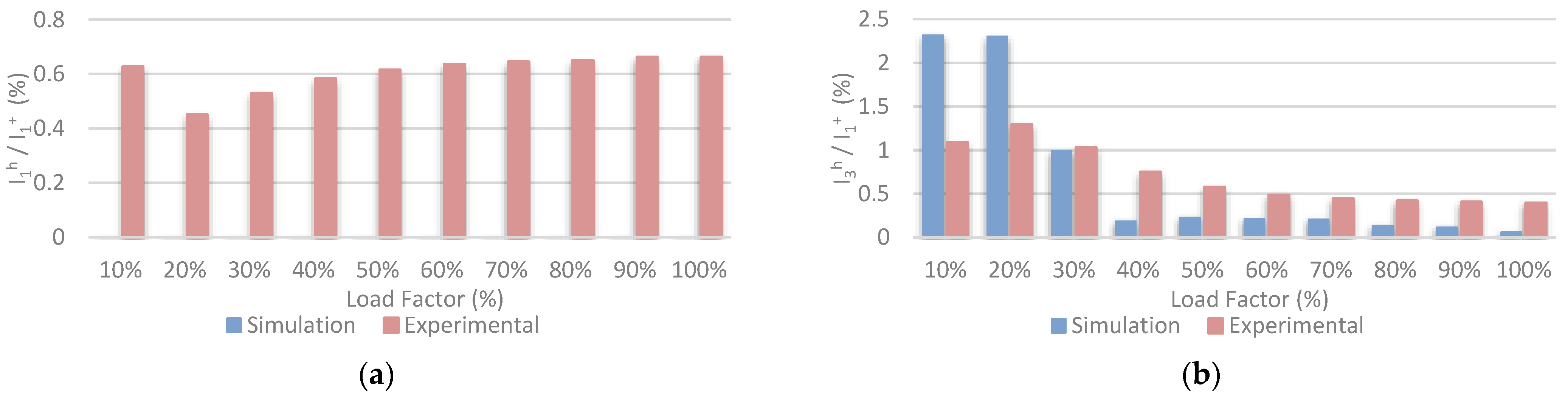
Figure 11.
Simulation and experimental harmonics of: (a) 50 Hz I1h/I1+; and (b) 150 Hz I3h/I1+ in the whole range of power of the circulating current with unbalanced load factor between inverter #1 and #2.
Figure 11.
Simulation and experimental harmonics of: (a) 50 Hz I1h/I1+; and (b) 150 Hz I3h/I1+ in the whole range of power of the circulating current with unbalanced load factor between inverter #1 and #2.
Figure 12.
Circulating current with a 40% increase in the inductance of phase A of inverter #2. Phase currents of inverter #1 at the top, circulating currents in the middle, and phase currents of inverter #2 at the bottom: (a) 100% load factor simulation results; (b) 100% load factor experimental results.
Figure 13.
Simulation and experimental harmonic of 50 Hz I1h/I1+ in the whole range of power of the circulating current with a 40% increase in the inductance of phase A of inverter #2.
Figure 13.
Simulation and experimental harmonic of 50 Hz I1h/I1+ in the whole range of power of the circulating current with a 40% increase in the inductance of phase A of inverter #2.
Figure 14.
Circulating current with SVM in inverter #1 and SPWM in inverter #2. Phase currents of inverter #1 at the top, circulating currents in the middle, and phase currents of inverter #2 at the bottom: (a) 100% load factor simulation results; (b) 100% load factor experimental results.
Figure 14.
Circulating current with SVM in inverter #1 and SPWM in inverter #2. Phase currents of inverter #1 at the top, circulating currents in the middle, and phase currents of inverter #2 at the bottom: (a) 100% load factor simulation results; (b) 100% load factor experimental results.
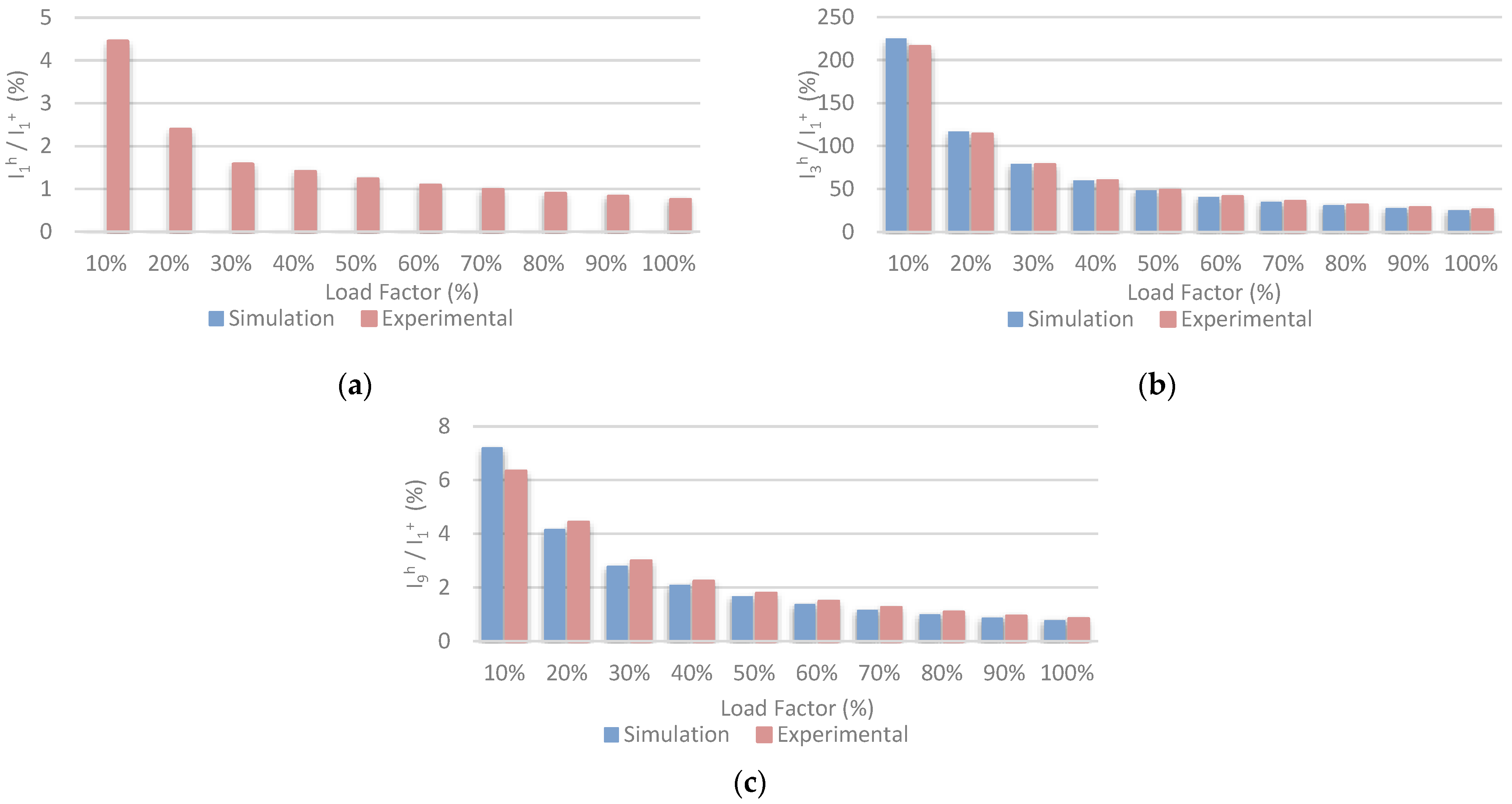
Figure 15.
Simulation and experimental harmonics of: (a) 50 Hz I1h/I1+; (b) 150 Hz I3h/I1+; and (c) 450 Hz I9h/I1+ in the whole range of power of the circulating current with SVM in inverter #1 and SPWM in inverter #2.
Figure 15.
Simulation and experimental harmonics of: (a) 50 Hz I1h/I1+; (b) 150 Hz I3h/I1+; and (c) 450 Hz I9h/I1+ in the whole range of power of the circulating current with SVM in inverter #1 and SPWM in inverter #2.
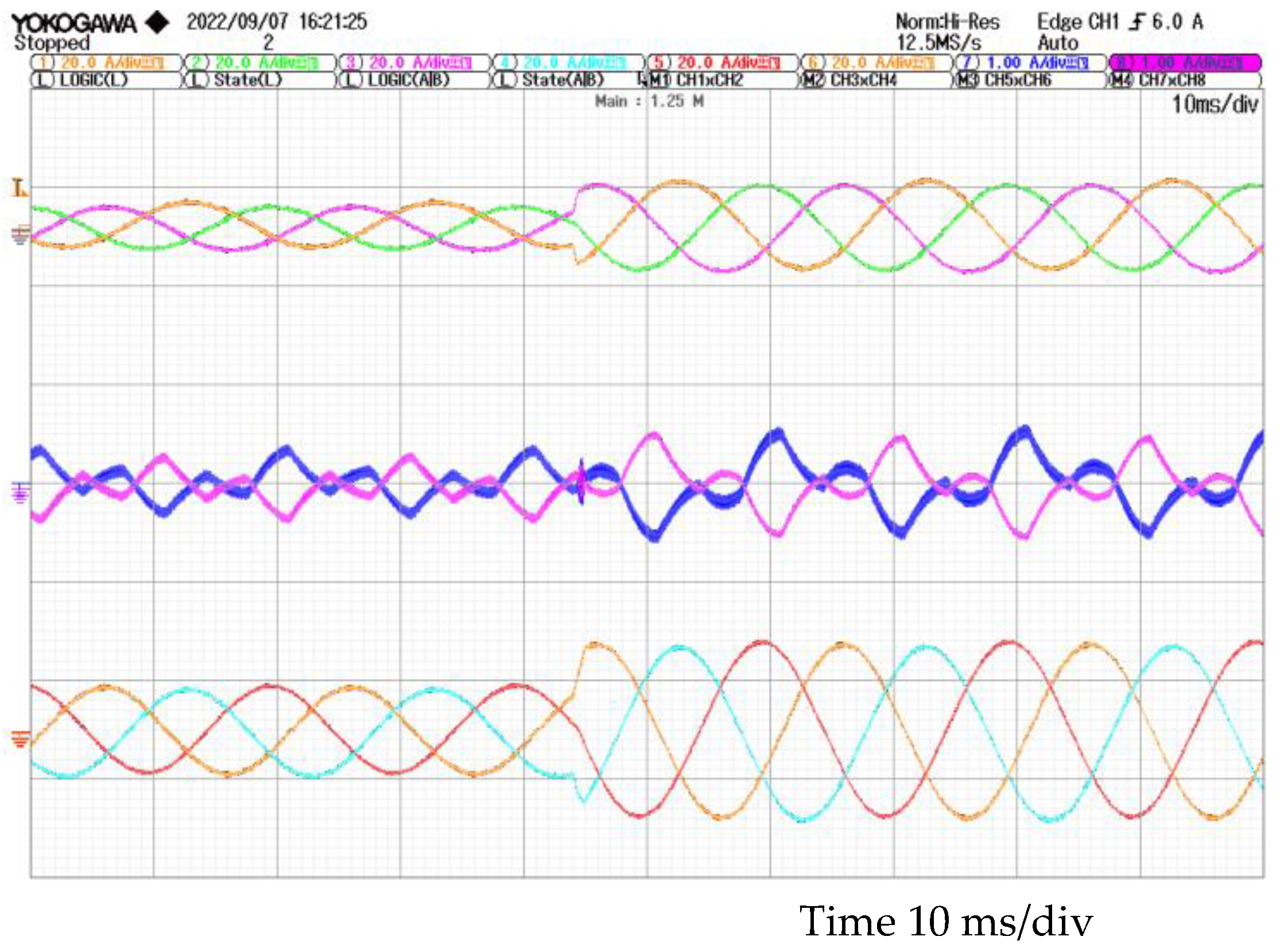
Figure 16.
Experimental circulating current with a load step from 25% to 50% in inverter #1 and from 50% to 100% in inverter #2. Phase currents of inverter #1 at the top, circulating currents in the middle, and phase currents of inverter #2 at the bottom.
Figure 16.
Experimental circulating current with a load step from 25% to 50% in inverter #1 and from 50% to 100% in inverter #2. Phase currents of inverter #1 at the top, circulating currents in the middle, and phase currents of inverter #2 at the bottom.
Figure 17.
Experimental circulating current with a load step from 50% to 100% when the inductance of phase A of inverter #2 is increased by 40%. Phase currents of inverter #1 at the top, circulating currents in the middle, and phase currents of inverter #2 at the bottom.
Figure 17.
Experimental circulating current with a load step from 50% to 100% when the inductance of phase A of inverter #2 is increased by 40%. Phase currents of inverter #1 at the top, circulating currents in the middle, and phase currents of inverter #2 at the bottom.
Figure 18.
Experimental circulating current with a load step from 50% to 100%when inverter #1 is controlled by SVM and inverter #2 by SPWM. Phase currents of inverter #1 at the top, circulating currents in the middle, and phase currents of inverter #2 at the bottom.
Figure 18.
Experimental circulating current with a load step from 50% to 100%when inverter #1 is controlled by SVM and inverter #2 by SPWM. Phase currents of inverter #1 at the top, circulating currents in the middle, and phase currents of inverter #2 at the bottom.
Figure 19.
High-power photovoltaic inverters connected in parallel.
Figure 19.
High-power photovoltaic inverters connected in parallel.
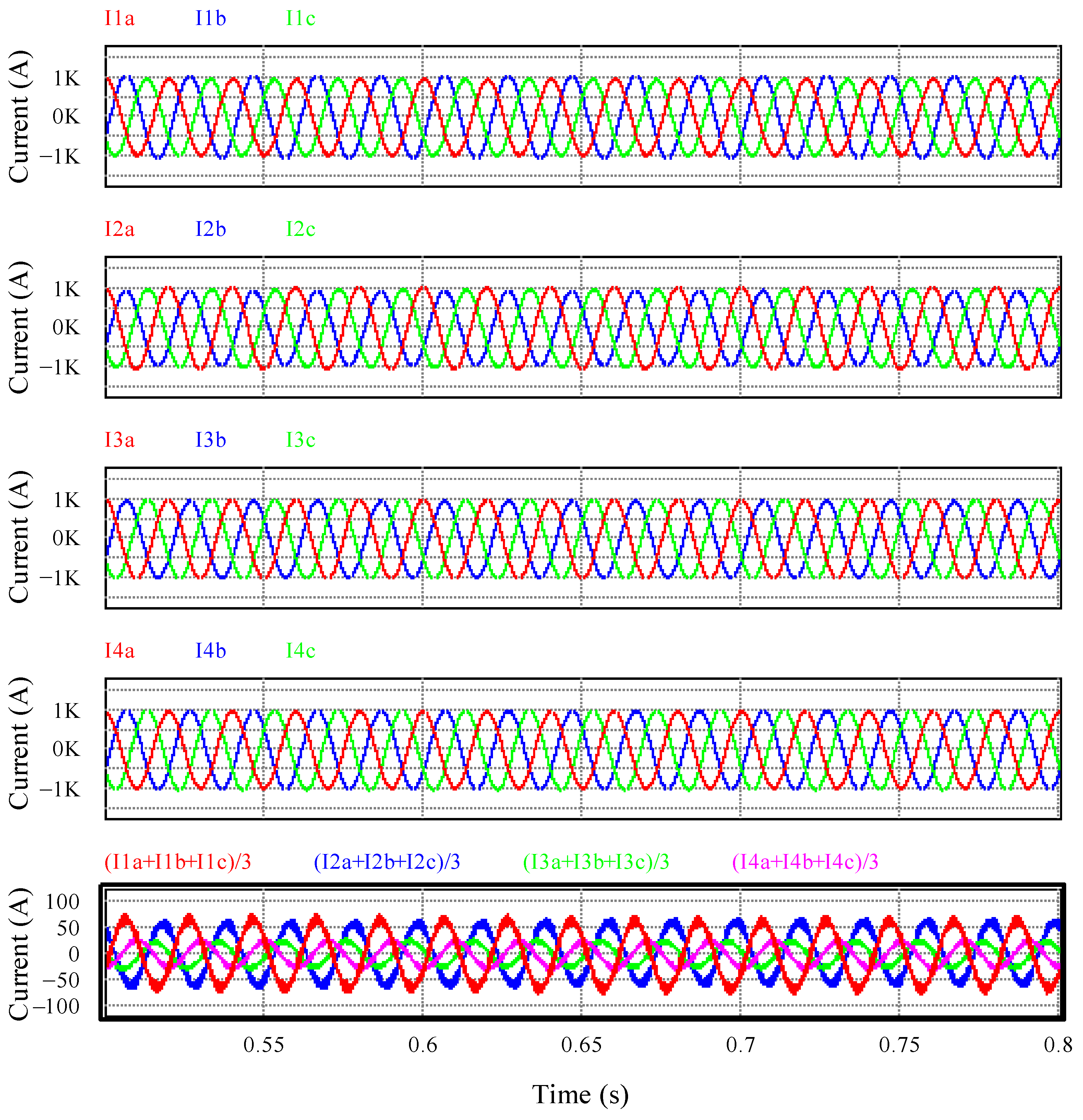
Figure 20.
Circulating currents in high-power photovoltaic farms. From top to bottom, phase currents in inverters #1, #2, #3, and #4 and circulating currents.
Figure 20.
Circulating currents in high-power photovoltaic farms. From top to bottom, phase currents in inverters #1, #2, #3, and #4 and circulating currents.
Table 1.
System parameters.
Table 1.
System parameters.
| Parameter | Nominal Value | Parameter | Nominal Value |
|---|
| Vg-RMS (phase-phase) | 230 V | Mb | −80 µH |
| Vdc | 500 V | ra | 50 mΩ |
| Pn | 5 kW | rb | 50 mΩ |
| fg | 50 Hz | Cf | 9 µF |
| Co | 1.2 mF | Rd | 4.4 Ω |
| La | 5 mH | fsw | 10 kHz |
| Lb | 320 µH | | |
Table 2.
Measured values of inductances La.
Table 2.
Measured values of inductances La.
| Parameter | Nominal Value | Parameter | Nominal Value |
|---|
| La_a1 | 5.14 mH | La_a2 | 5.1 mH |
| La_b1 | 5.14 mH | La_b2 | 4.85 mH |
| La_c1 | 5.27 mH | La_c2 | 5.03 mH |
Table 3.
Real inductance values.
Table 3.
Real inductance values.
| Parameter | 5-mH Inductor | Parameter | 5-mH Inductor | 2-mH Inductor | 7-mH Total Inductance |
|---|
| La_a1 | 5.14 mH | La_a2 | 5.1 mH | 2.06 mH | 7.16 mH |
| La_b1 | 5.14 mH | La_b2 | 4.85 mH | 2.13 mH | 6.98 mH |
| La_c1 | 5.27 mH | La_c2 | 5.03 mH | 2.09 mH | 7.12 mH |
Table 4.
Value of inductances la with a 40% imbalance in phase A of inverter #2.
Table 4.
Value of inductances la with a 40% imbalance in phase A of inverter #2.
| Parameter | Nominal Value | Real Value | Parameter | Nominal Value | Real Value |
|---|
| La_a1 | 5 mH | 5.14 mH | La_a2 | 7 mH | 7.16 mH |
| La_b1 | 5 mH | 5.14 mH | La_b2 | 5 mH | 4.85 mH |
| La_c1 | 5 mH | 5.27 mH | La_c2 | 5 mH | 5.03 mH |
Table 5.
Parameters of the high-power photovoltaic inverters.
Table 5.
Parameters of the high-power photovoltaic inverters.
| Parameter | Nominal Value | Parameter | Nominal Value |
|---|
| Vg-RMS (phase-phase) | 400 V | Mb | −15 µH |
| Vpv | [650–820] V | Mc | 0 |
| Pn | 500 kW | ra | 1 mΩ |
| fg | 50 Hz | rb | 1 mΩ |
| Co | 15 mF | rc | 1 mΩ |
| La | 160 µH | Cf | 500 µF |
| Lb | 60 µH | Rd | 0.12 Ω |
| Lc | [2.5–50] µH | fsw | 2 kHz |
| Ma | −40 µH | | |
Table 6.
Comparison with previous works.
Table 6.
Comparison with previous works.
| Mismatches | Inductances (Different Inverters) | Load Factor | Voltage Frequency | Voltage Phase | Inductances (Same Inverter) | Phase Shift PWM | Modulation Technique |
|---|
| Results obtained in this work |
| I1h/I1+ | 0.01% | 0.644% | - | - | 6.68% | - | 0.98% |
| I3h/I1+ | 0.03% | 0.44% | - | - | 0.007% | - | 35.41% |
| IZ RMS | 0.057 A | 0.08 A | - | - | 0.697 A | - | 3.14 A |
| THDi Ia | 0.58% | 1.25% | - | - | 0.64% | - | 30.91% |
| Previous work [27] |
| I1h/I1+ | - | - | - | - | - | 1.83% | - |
| I3h/I1+ | - | - | - | - | - | 6.25% | - |
| IZ RMS | - | - | - | - | - | 0.88 A | - |
| THDi Ia | - | - | - | - | - | - | - |
| Previous work [28] |
| I1h/I1+ | - | - | - | - | - | - | - |
| I3h/I1+ | - | - | - | - | - | - | - |
| IZ RMS | - | - | 0.096 A | 0.24A | - | - | - |
| THDi Ia | - | - | - | - | - | - | - |

 ,
, 


