1. Background
Clinical ECG consists of 12 leads (S12)—namely limb leads I, II, and III, augmented leads aVR, aVL, aVF, and precordial leads V1 through V6. Vectorcardiography (VCG) [
1] is complementary to the S12. It is essentially the spatiotemporal representation of the cardiac vector in 3 orthogonal planes—namely vertical, transverse, and sagittal planes. S12 is the standard whereas VCG is rarely acquired. However, several conditions have more prominent VCG changes than S12, so it is a useful complement to S12. Furthermore, dynamic spatial and temporal information that can be derived from VCGs is unavailable from an ECG, which may enhance the automatic assessments of cardiovascular diseases [
2].
Ernest Frank introduced the XYZ lead system known as vectorcardiography to provide a 3-dimensional representation of the cardiac vector.
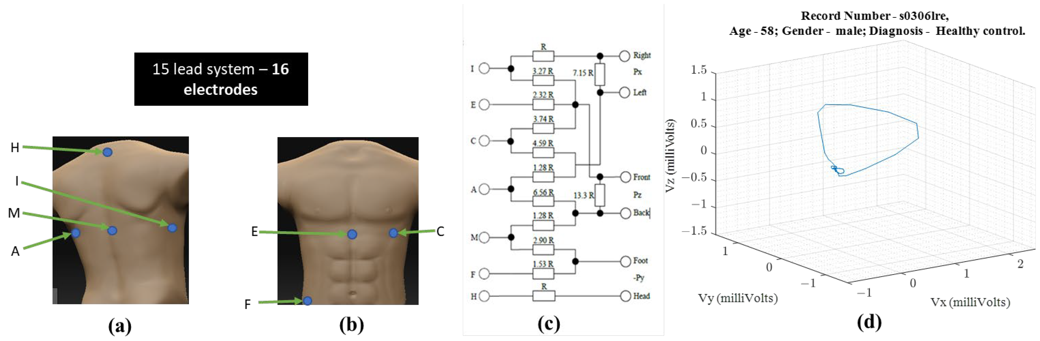
Figure 1 shows the electrode placement for vectorcardiogram and an example of a vectorcardiogram tracing for a healthy male subject.
Following the illustration in
Figure 1, a vector tracing the boundary of this 3D object circumscribed by the vectorcardiography is the cardiac vector. Ideally, these ECG leads—X, Y, and Z—would be orthogonal to each other and form a basis for the cartesian space spanned by the cardiac vector.
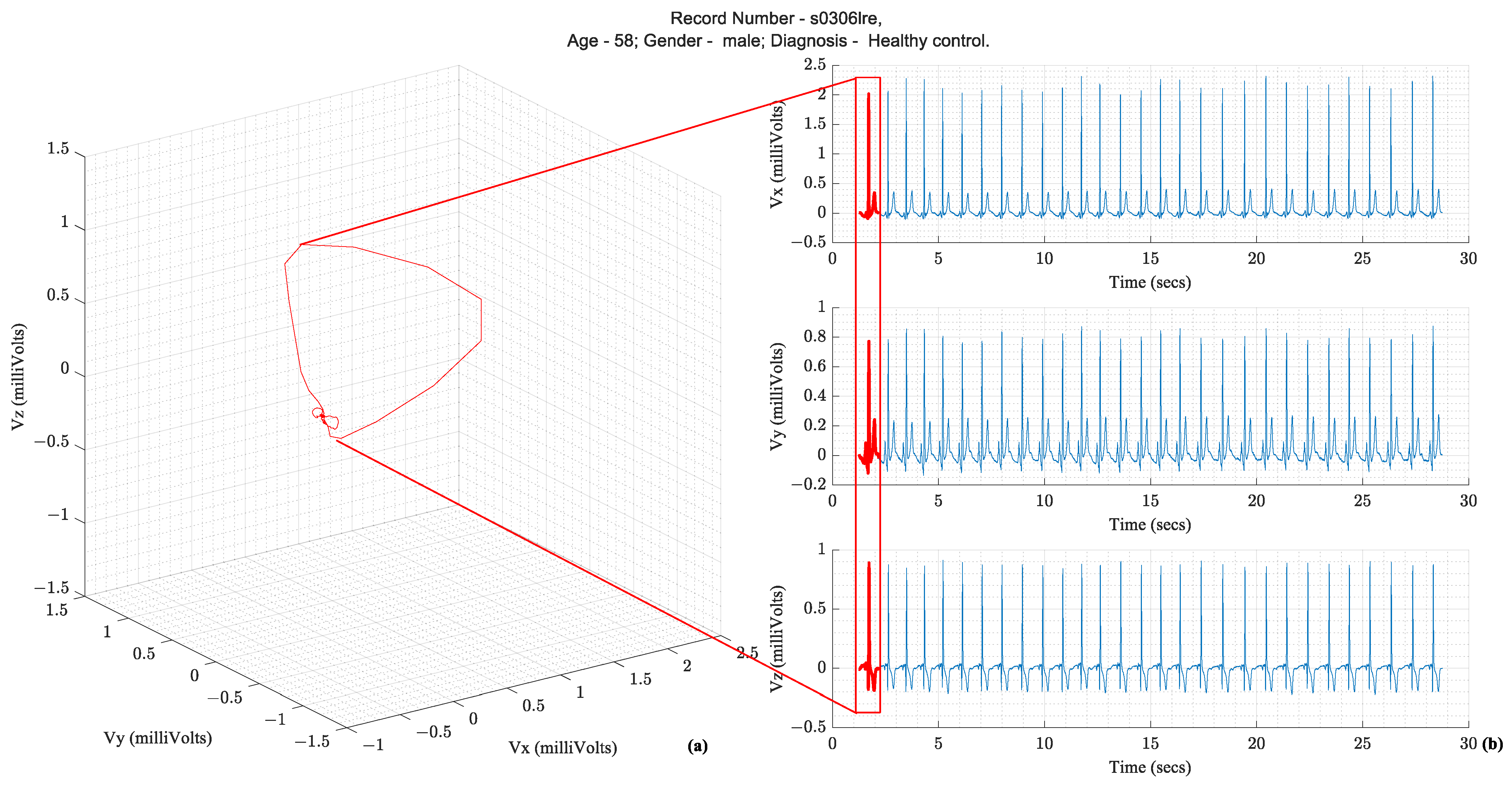
Figure 2 illustrates how the temporal X, Y, and Z lead waveforms translate to a spatiotemporal VCG.
The S12 requires ten electrodes on the skin while the Frank XYZ requires only 7 electrodes. There is only one electrode position in common (i.e., the left leg). Suppose all 15 leads are to be recorded with an ECG acquisition system, then sixteen electrodes should be placed on the patient’s skin. Another practical issue with the location of the Frank XYZ electrodes is the rear electrodes. Patients can sleep on their backs, but having cables on their backs can be uncomfortable.
1.1. Diagnostic Importance of VCG and Its Complementarity to ECG
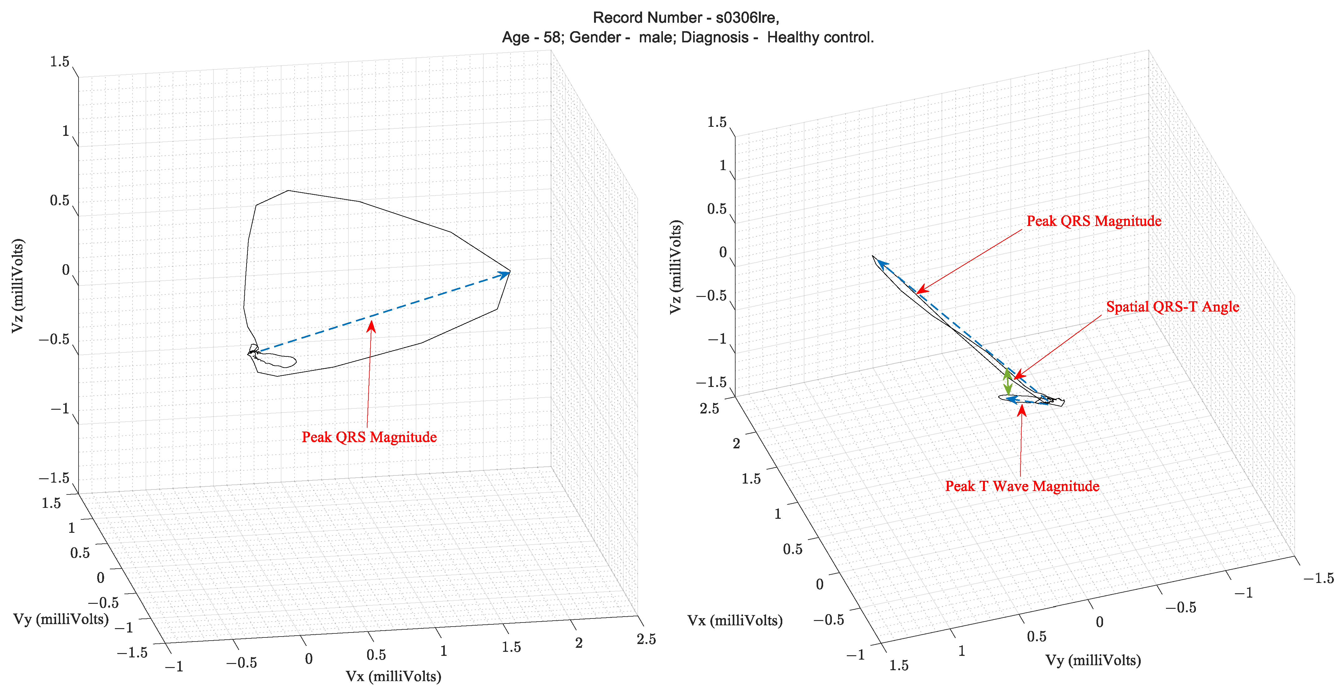
Over several decades of research, three parameters extracted from the VCG waveform are considered diagnostically important. They are the QRS amplitude, T-loop magnitudes, and Spatial QRS-T loop angles.
Figure 3 illustrates these parameters on a vectorcardiogram.
Table 1 lists the clinical applications of these parameters that have been validated in the literature. The spatial QRS-T angle parameter has been shown to be useful for risk stratification for cardiac events, evaluation of incident coronary disease and heart failure, and efficacy of therapy for adult hypertension and diabetes mellitus [
5]. For example, in the PTB diagnostic database [
3,
4] ECG used in this study, the mean and standard deviation of the Spatial QRS-T angles from patients with MI and healthy controls were 87.9° ± 46.84° and 52.95° ± 35.76°, respectively, as computed using the VCG parameter extraction algorithms described in this study.
Additionally, there are specific conditions where the VCG is considered superior to the ECG. VCG is more sensitive and specific than ECG in detecting atrial and ventricular enlargements. Due to the greater spatially localized information in a VCG, the suspicion of electrically inactive areas in the septal or anteroseptal walls of the left ventricle can be assessed with a VCG. The left ventricular mass, which is currently assessed with an echocardiogram, can be assessed with a VCG. VCG findings are better correlated to echocardiography findings than ECG findings. VCG has a greater diagnostic sensitivity than ECG for AMI when associated with a left anterior fascicular block [
6]. Lastly, the myocardial damage caused by Chagas disease can be assessed with VCG findings complementing ECG findings [
7].
Figure 4 illustrates the conditions and the location of the affected heart anatomy.
Since VCGs are not acquired during regular clinical settings, but standard 12-lead waveforms are acquired, there is a need to derive VCG from the 12-lead ECG. Specifically, an arbitrarily complex transformation mapping the 12-lead ECG to the VCG is needed. Several research efforts are focused on arriving at the linear transformation of ECGs from standard 12-lead to Frank XYZ. However, the transformation is likely to be arbitrarily complex due to multiple underlying variabilities from person to person in terms of the distribution of fat, muscle, and organs in the torso where the ECG leads are measured. These complex variations suggest that we need methods capable of approximating arbitrarily complex transformations, such as neural networks [
8,
9]. Therefore, we used a class of neural networks, namely Long Short-term Memory (LSTM) [
10,
11], that might be best suited for time-series data regression tasks, such as transforming leads. Moreover, most recently, Sohn et al. [
12] reported the successful use of LSTM networks to achieve accurate lead transformations. The following are the original contributions of this research:
We apply LSTM networks to the task of deriving VCG from 12-lead ECGs. Since LSTM networks require the pre-specification of several hyperparameters, we apply Bayesian global optimizations to find the combination of these parameters that is optimal to obtain the least error between derived VCG and actual VCG;
We apply transfer learning to obtain personalized transformations for each subject as part of the data set;
We compare the accuracy of extraction of VCG diagnostic parameters from derived VCG and actual VCG.
1.2. Related Work
Linear regression has been explored in the literature for lead transformation. Some studies have used open, publicly available data sets, whereas others have used closed data sets or data sets acquired with custom built hardware devices. Between 1986 and 2009, the lead transformation of interest was from S12 to Frank XYZ. Closed data sets were used for some studies [
13,
14,
15,
16] and open for others [
17,
18]. A neural network-based transformation was first proposed in 2010 [
19].
Table 2 summarizes the works in the literature that focused on obtaining Frank XYZ from S12. Since then, several efforts have been made in reducing leads required to be monitored while retaining the diagnostic power of S12. Most of the studies have tried to derive S12 from a three-lead ECG [
12,
19,
20,
21,
22,
23,
24].
Several studies have used closed data sets that are unavailable to other researchers. We used the PTB diagnostic ECG repository for this study [
3,
4].
The Root Mean Square (RMS) and correlation coefficient are the most commonly reported metrics used to evaluate the error between generated or derived ECG compared to the ground truth waveform. In the literature, R-squared is used.
Table 2 includes the definitions and equations of these metrics. Some clinically relevant VCG-derived parameters can also be compared between the derived ECG leads and the ground truth waveform. Therefore, the RMS error, correlation coefficient, R
2, QRS amplitude or magnitude, T wave amplitude or magnitude, and spatial QRS-T angle form a complete assessment.
2. Materials and Methods
2.1. Experimental Setup
We had previously presented the methodology of training a generalized model and then applying transfer learning for a different problem, which was for the S12 lead ECG derivation from a subset of leads, namely Lead II, V2, and V6 [
25]. However, in this paper, we evaluate the performance of the transformations from S12 lead to Frank XYZ lead. We present the methodology here for the convenience of the reader. All data analysis programs and applications were implemented using MATLAB 2021a Update 5 version 9.10.0.1739362 (MathWorks Inc., Natick, MA, USA) on a system with an Intel processor (i7-7820X), RTX 3090 graphics processing unit (NVIDIA Corp., Santa Clara, CA, USA), and 32 GB of RAM.
2.1.1. Source of Data and Data Preparation
The PTB ECG database available on Physionet [
3,
4] contains fifteen lead ECGs sampled at 1 kHz from 249 patients. Some patients have multiple records, bringing the total number of ECGs to 549.
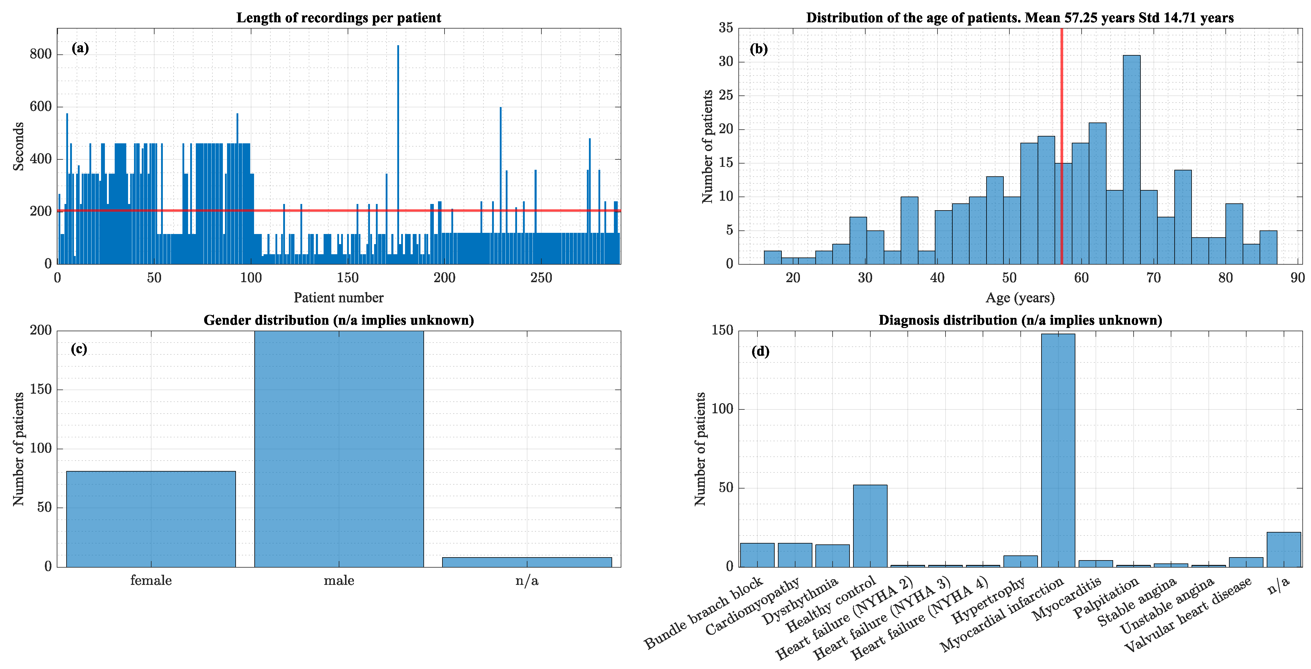
Figure 5 plots the histograms that summarize the data set’s characteristics.
This data set contains only one diagnosis per patient. As shown in
Figure 5, a large proportion of the data set is MI patients and healthy controls.
The ECG signals were band pass filtered using a second order Butterworth filter with a passband from 0.05 Hz to 45 Hz, which is the bandwidth used for long-term rhythm monitoring according to AAMI standards [
26]. Following filtering and suppression of frequencies beyond 40 Hz, the signal was down sampled using decimation to avoid aliasing effects. First, ECG signal content in adults was below 100 Hz [
26], so 200 Hz satisfied the Nyquist rate requirements to avoid aliasing. Second, lower sampling rates reduced the amount of data so iterations could be faster.
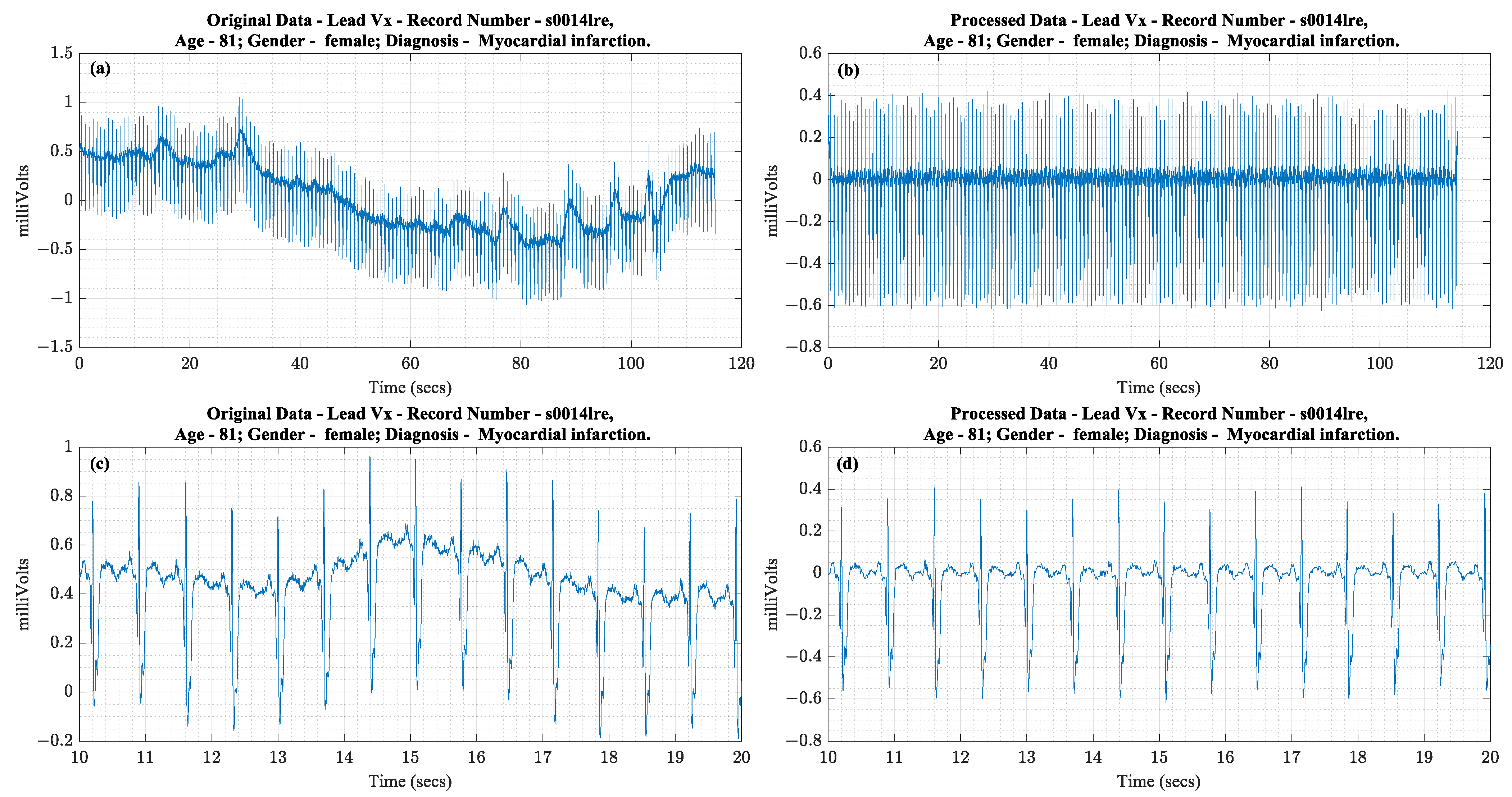
Figure 6 shows an example of a recording from the data set before and after applying the above-stated data preparation steps. The data processing steps cause no visible distortion.
Three recordings were removed from the data set because of missing data or complete data corruption by noise.
Table 3 lists them and the reason for exclusion.
2.1.2. Personalized Training Data Preparation
Data augmentation was performed using the sliding window method as used in [
12]. Each sliding window was 17 s, and the overlap size was 16 s. We chose a window size of 17 s solely for formatting and initial review purposes for the S12 leads. We required 12 s of data to chart S12 in a standard clinical ECG format. We also had symmetrically cropped 2.5 s of data on both ends of each 17-s-long segment so that we could be consistent across all segments. The beginning and end of several records had settling noise, such as baseline wander or powerline noise, so we removed these segments during data preparation. The 16 s overall was chosen to maximize overlap and number of training samples available following similar approaches in the literature that showed good performance using LSTM.
2.2. Neural Network Architecture
As mentioned earlier in
Section 1.2, we used LSTM neural networks to learn a transfer function from S12 to Frank XYZ. The principal constituents of the LSTM network were the input gate (
), forget gate (
), and output gate (
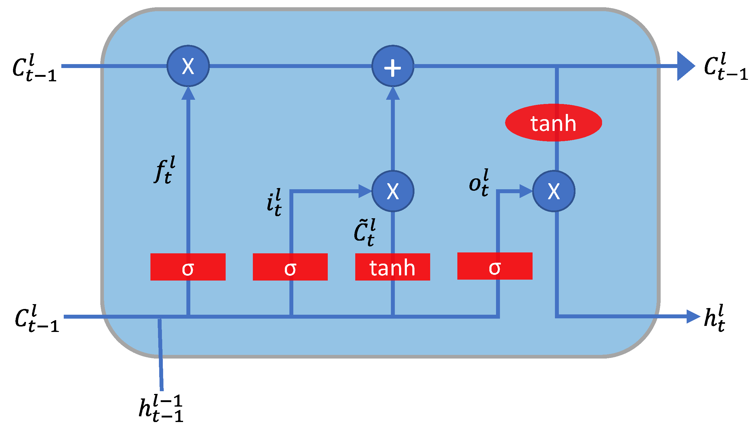
). In addition, each LSTM network consisted of a cell state that was updated upon each timestep of input presented to the network.
The LSTM cell is a type of recurrent neural network. The output at time
influences the output at time
.
Figure 7 presents a depiction of a single LSTM cell.
The training process for the LSTM neural network involved a standard four-step sequence: forward propagation, cost computation, backward propagation, and weight update. This process was repeated for each item in the training set multiple times. The loss function was the mean squared error without normalization of the number of output dimensions or the number of ECG channels. Weight updates were performed using Adam optimizer [
27].
where
was sequence length of each ECG channel,
equaled the number of ECG channels in the output,
was the instantaneous estimated output, and
was the instantaneous actual sample of ECG.
The LSTM network required selection of the following list of hyperparameters and architecture specifications prior to training—number of layers, number of hidden units per layer, learning rate, minibatch size, learning rate schedule (i.e., periodic changes as training progresses or fixed with no changes), and finally, the weight optimizer parameters—momentum coefficient ( and root mean square (RMS) propagation coefficient (
The LSTM network architecture requires the specification of a list of hyperparameters. Bayesian optimization (BO) is a global optimization approach that is preferred in the literature for computationally intensive functions like the training of neural network [
28].
2.3. Network Training Options
The 546 available records were split 80/20 between training and testing. The training set had 437 records, and the test had 109. Network training was performed over 100 epochs for all networks, including the personalized networks.
BO did not include number of layers as an optimizable variable, so we were able to infer the meaning of the number of layers in a controlled way rather than as part of a probabilistic search like BO. Therefore, independent hyperparameter tuning was performed for 1- through 5-layer networks and the results were compared across the number of layers to understand the impact of multiple LSTM layers on performance.
Hyperparameter Optimization Using BO
BO was used to find the optimal combination of values for the hyperparameters needed for the LSTM networks. The application method of BO included three key elements:
A Gaussian Process Model ()—final validation RMSE was the objective function . The kernel function for the model was ARD Matérn 5/2;
A procedure for updating () after each iteration;
An acquisition function
that was ‘expected improvement’ [
29].
where
was the minimum of the posterior mean and
was the location of this minimum in hyperparameter space. To boost the inclination for sampling
and prevent over-sampling of a region within the hyperparameter space around a local minimum of
, another criterion was added in addition to the one used to select
. This condition was implemented as an additional restriction when choosing the subsequent
for evaluation. A candidate
had to satisfy the criteria in (3) to be selected as the subsequent point to be evaluated.
where
represented the standard deviation of the posterior objective function at
and
the additive noise’s posterior standard deviation.
The optimizable variables or the hyperparameters had to be defined in terms of bounds and the type of transformation to be applied prior to sampling.
Table S2 in the Supplementary Materials lists the hyperparameters optimized for networks ranging from 1-layer to 5-layer. For each objective function evaluation, networks were trained for 100 epochs to allow adequate iterations to reach the lowest final RMSE.
2.4. Training Personalized Networks
Transfer learning is the process of further training a pre-trained neural network using a different data set or subset of data [
30]. We trained a personalized neural network for each patient using transfer learning with the optimal network architecture and hyperparameter combinations found by BO. The data set had 549 ECG recordings from 290 patients, averaging 200 s per recording, with a few patients having only 100 s of data.
As described in
Section 2.1.2, network training was performed over 100 epochs with personalized data.
2.5. Evaluation of Extracted VCG Parameters
As described previously in
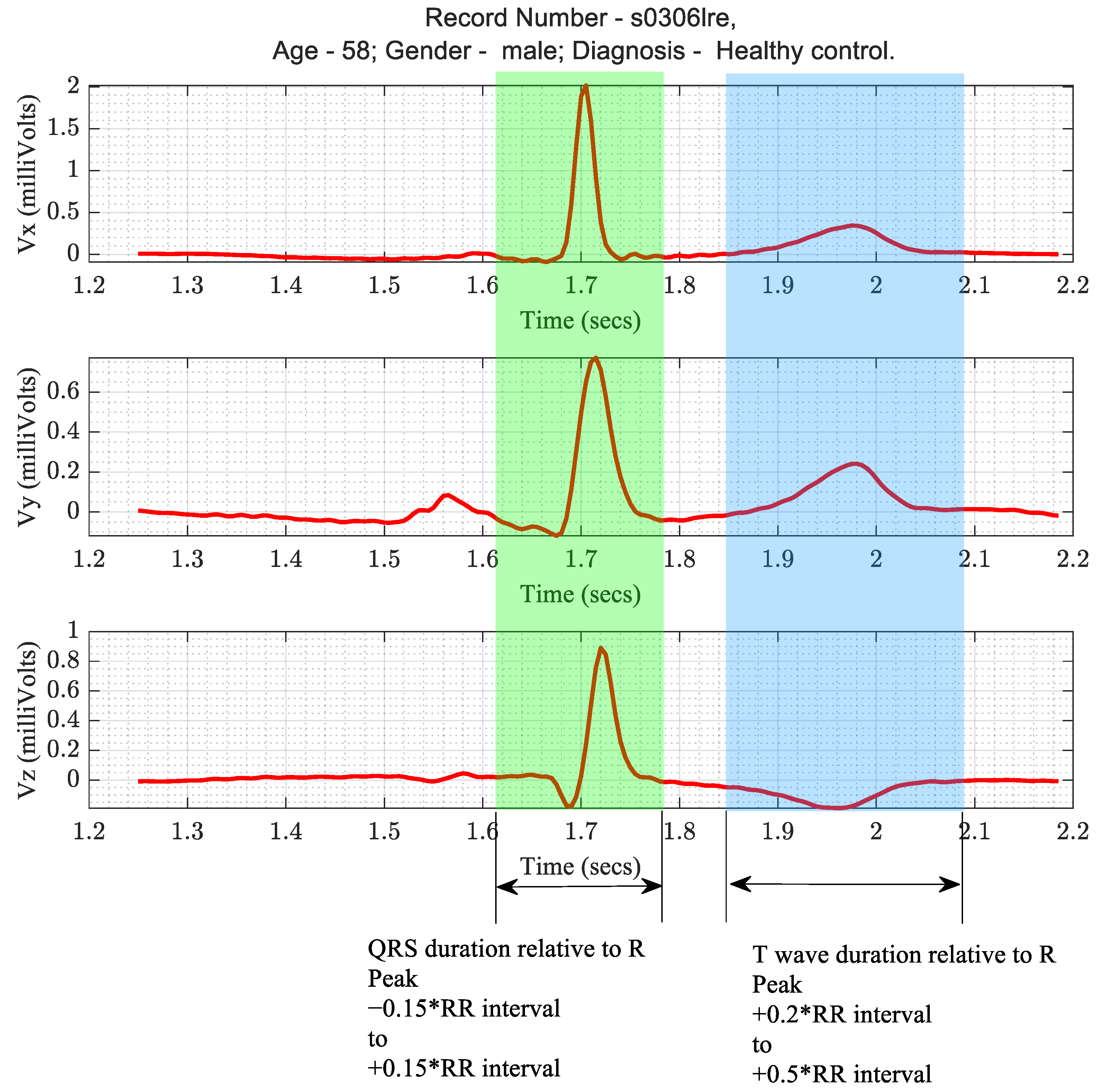
Section 1.1, three VCG extracted parameters—peak QRS magnitude, peak T wave magnitude, and spatial QRS-T angle—were of diagnostic importance. These parameters were computed from the actual Frank XYZ leads and the derived Frank XYZ leads from all the transformations. The algorithm for calculating these parameters began with the detection of the R wave of the ECG in the Vx lead. The QRS duration and the R wave durations were defined relative to the corresponding RR interval, as depicted in
Figure 8.
The peak magnitudes of QRS were calculated as the maximum of the L2 norm of (V
x, V
y, V
z) within the QRS duration time window. Similarly, the maximum within the T wave duration time window was the peak T wave magnitude. The QRS-T angle was computed using Equations (4) through (6).
where
,
, and
were the area under the curve of the QRS complex in the
X,
Y, and
Z leads, respectively, and
,
, and
were the area under the curve of the
T wave in the
X,
Y, and
Z leads, respectively. Several possible integration methods (for example, the Trapezoidal rule, the Simpson’s rule, or the Simpson’s 3/8) could be used to calculate the area [
31]. In this implementation, we used the trapezoidal rule. We compared the extracted parameters using Pearson’s correlation coefficient and Bland Altman limits of agreement.
3. Results
As part of the BO experiment, we trained 250 neural networks: 50 networks each for 1- through 5-layer networks.
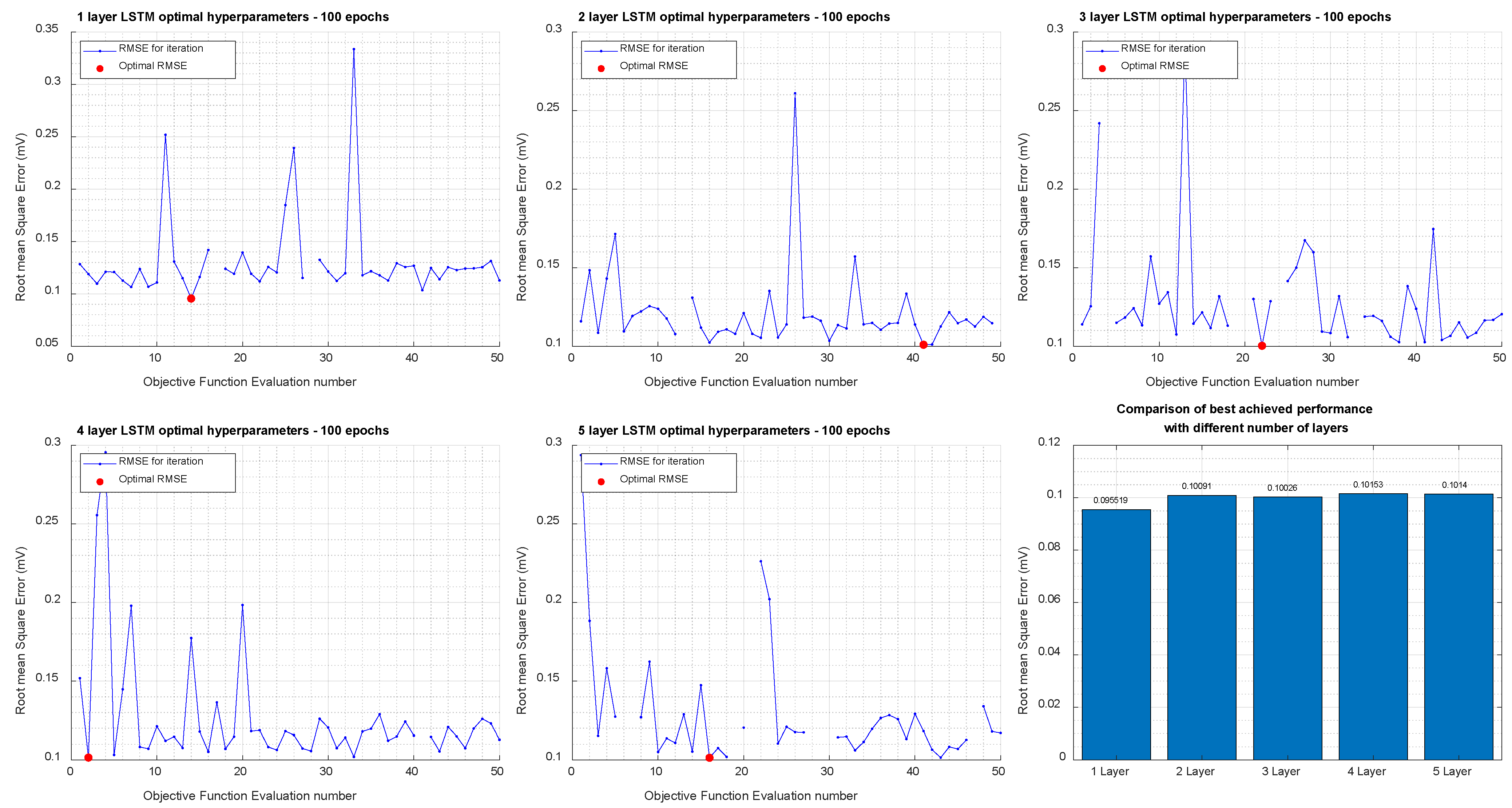
Figure 9 shows the overall results of the BO for 1-to-5-layer neural networks to transform ECG leads from S12 to Frank XYZ leads. The following were the set of hyperparameters that resulted in the optimal Final RMSE: Number of Hidden Units = 47; Mini Batch Size = 27; Learning rate schedule = Piecewise;
= 0.90025;
= 0.90035; and Learning Rate = 0.062561.
The 1-layer network was found to have the lowest validation RMSE (0.0955 mV). Overall, there is an insignificant difference between the RMSE across the number of layers. The best RMSE and the worst RMSE differ by only 5 µV.
3.1. Comparison of Performance Metrics
The metrics for quantitative comparison of waveforms in this study were RMSE, R
2, and Pearson correlation coefficient.
Table 4 provides the results for all the methods of transformation implemented in this study.
3.2. Comparison of Extracted Diagnostic Parameters
As described in
Section 2.5, three diagnostic features of the VCG waveform were computed from the actual and derived XYZ waveform data. The features computed from the actual data are treated as actual measurements, and those computed from the derived data are treated as measurements from a test device or methodology. In this case, the methodology is the transformation of ECG leads through a general and patient-specific personalized model. The metrics used for comparison are Pearson’s correlation coefficient and the Bland-Altman limits of agreement [
32]. We further present the effect size for comparison of VCG parameters from each transformation method and actual VCG. The effect size metrics include Cohen’s U1, U3 [
33], and common language effect sizes [
34]. We also present
t-test results with t-statistic and the associated
p-value. The
t-test
p-values in this case should be greater than 0.05 if we are to accept the null hypothesis that the difference in means is not significant (i.e., the transformation method yielded results for VCG parameters that were comparable or similar to those obtained from the actual VCG).
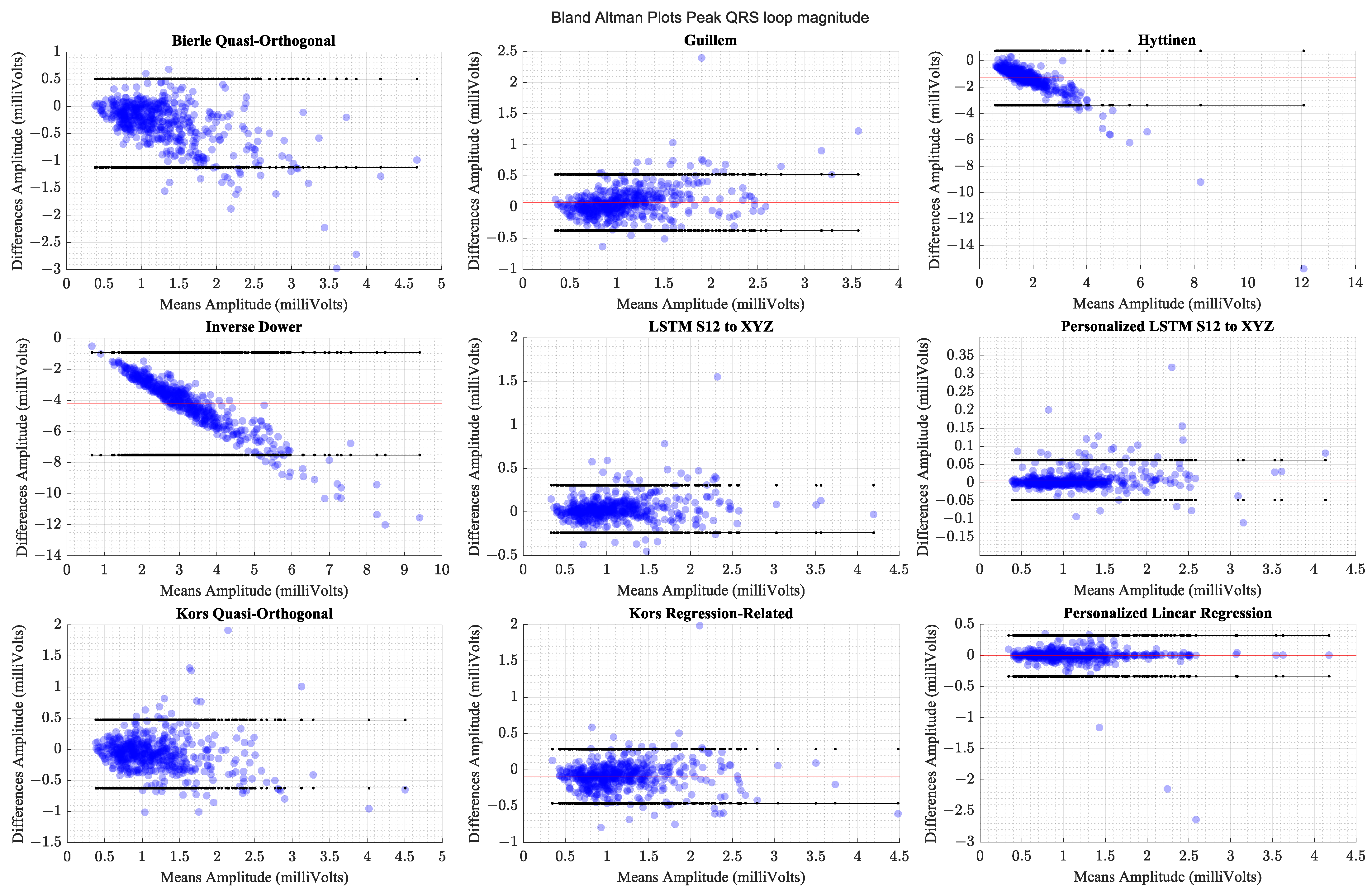
3.2.1. Peak QRS-Loop Magnitude
The personalized models showed the highest correlation coefficient values and the smallest limits of agreement, indicating that the derived peak QRS magnitudes were closest to the values computed from the actual data.
Table 5 lists the correlation coefficients for the different transformation methods in descending order along with the statistical measures of comparison and effect sizes.
Table 6 presents the Bland–Altman limits of agreement between QRS-loop magnitudes extracted from actual and derived VCG waveforms.
Figure 10 presents the Bland-Altman plots for QRS-loop magnitude comparison.
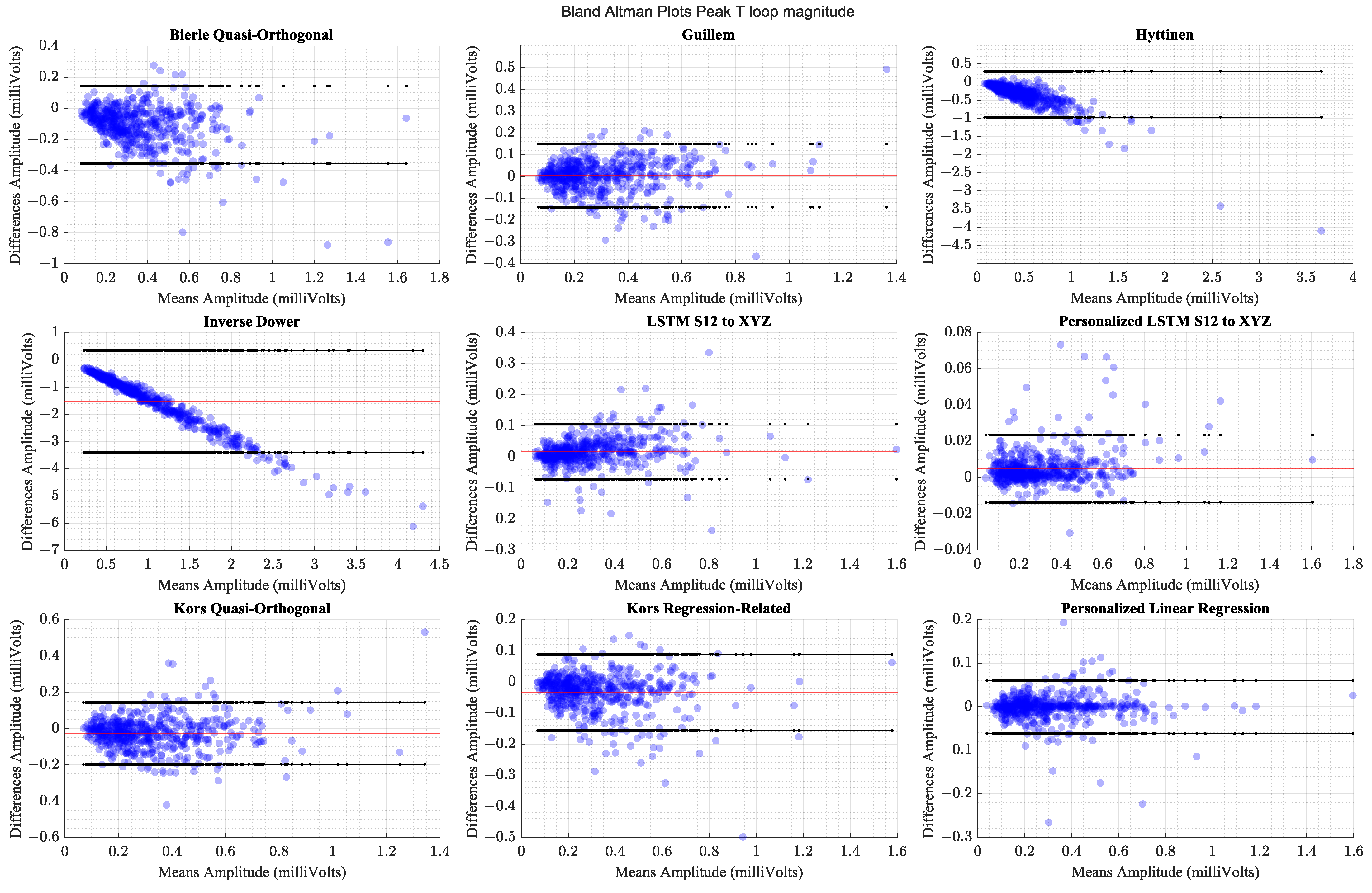
3.2.2. Peak T-loop Magnitude
The personalized models show the highest correlations and the smallest limits of agreement. The generalized models perform comparably to the better performing transforms from the literature.
Table 7 shows the methods’ respective correlation coefficients sorted in descending order along with the statistical measures of comparison and effect sizes.
Table 8 presents Bland–Altman Limits of Agreement between the peak T-loop magnitudes computed from the actual VCG waveforms and the derived waveforms across different methods of derivation.
Figure 11 presents the Bland -Altman plots for the comparison of Peak T-loop magnitude.
3.2.3. Mean Spatial QRS-T Angle
The personalized models show the highest correlations and the smallest limits of agreement. The generalized models perform comparably to the better performing transforms from the literature.
Table 9 shows the methods’ respective correlation coefficients sorted in descending order along with the statistical measures of comparison and effect sizes.
Table 10 presents Bland–Altman limits of agreement between the mean QRS and T-loop spatial angle magnitudes computed from the actual VCG waveforms and the derived waveforms across different methods of derivation.
Figure 12 presents Bland-Altman plots for comparison of spatial QRS-T angle.
4. Discussion
The findings in this study indicate that personalized transformation models are preferable, but there are limitations to interpreting the results and practical considerations. The data set for this research is widely available, supporting further research and reproducibility of these results. However, the amount of data available is restricted to a small population that is not geographically or ethnically diverse. There is potential for overly optimistic results obtained in this study due to this aspect. Future studies should evaluate additional data sources from other geographic regions to confirm that these inferences are valid. Furthermore, there is only one diagnosis available per patient as the reason for hospitalization. ECG and VCG interpretations are unavailable. Comparisons on diagnostic yield and outcomes will require specific waveform interpretations, as well as longitudinal follow-up with patients so that we can evaluate how the clinical management of patients were impacted by the availability of VCG in addition to S12. In the absence of this information within the current data set, we could only evaluate the performance in terms of quantitative measures. We have presented effect sizes as statistical measures that could help with the evaluation of various transformation methods. However, there is no reasonable or equivalent comparison available in the literature thus far regarding an absolute interpretation of these results. The effect sizes can be compared across transformations in this study and reveal that generalized LSTM, personalized LSTM, and personalized linear regression perform better than other methods in that they have the least effect sizes when compared to the actual VCG in terms of values obtained for the VCG diagnostic parameters.
The findings indicate that personalized LSTM and personalized linear regression methods lead to nearly identical results with marginally better performance for personalized LSTM. Since the S12 leads cover the ventral plane of the body, it is plausible that the association between S12 and at least X and Y leads of VCG are nearly linear so that they can be derived using linear models. The comparisons between Z leads of VCG derived from the methods reveal a larger difference than X and Y leads. A future avenue of research may be to specifically explore Z-lead comparisons to understand if there is further scope for an improvement of performance with other lead transformation methods.
It is possible that neural network architectures other than LSTM may lead to better lead transformation performance. This study only explores LSTM and not the variants of LSTM. The choice of LSTM for this work was based on recent findings in the literature that demonstrated the use of this architecture to obtain acceptable results for the problem of lead transformations [
12]. Alternatively, this work explores personalization and its impact on lead transformation performance and LSTM architecture was evaluated. Several architectures can be explored in this manner for future research.
We had chosen to down sample and filter the ECG waveforms as part of the preprocessing step. There could be different findings if the ECGs were retained at the 1 kHz sampling rate and without filtering. Since the entire data set was preprocessed in the same manner, and all transformation methods were evaluated on the same data, there is no expectation that there would be bias in the results presented herein. However, an empirical evaluation of the impact of pre-processing may be beneficial to explore in a future study with the evaluation of sampling rate and signal conditioning approaches as the goal.
From a practical perspective, implementing the personalized models would require acquiring 15-lead ECGs for each patient, which is not currently part of standard care and would result in added costs and work for healthcare professionals. Furthermore, the data available in this data set is not longitudinal because no recordings span a time frame before and after a significant cardiovascular event. Longitudinal data of this kind must be used to validate the hypothesis LSTM networks as trained have adequately inferred the lead transformations following the subject’s anatomy.
Regarding the evaluation involving the extraction of VCG parameters, there is an underlying assumption that the algorithms were accurate. Therefore, we did not evaluate the performance of the algorithms alone. The use of the same algorithm for all data eliminates potential biases in comparisons, but further testing against a labeled VCG data set is necessary to assess the performance of the algorithms.
5. Conclusions
The personalized transformations performed better than generalized transformations in waveform comparisons and error performance of extracted diagnostic parameters from VCG waveforms. The use of personalized transformations for the derivation of VCG from S12 has the potential to improve and augment the diagnostic yield and accuracy of a S12 interpretation. The differences between personalized LSTM and linear regression transformation were marginally in favor of personalized LSTM. There were no statistically significant differences in the performance between them. A study focused on outcomes for patients and diagnostic yield is needed to evaluate the clinical impact of using such an approach for the derivation of VCG from S12 and using it as part of the patient management plan for a broader population. On balance, the results in this study suggest that personalization should be the preferred approach for ECG lead derivations.
Supplementary Materials
The following supporting information can be downloaded at:
https://www.mdpi.com/article/10.3390/eng4020078/s1, Table S1. Lists the coefficients for the linear transformation between Standard 12-lead ECG and Frank XYZ VCG; Table S2. Hyperparameter optimization variables, bounds, and sampling transformations.
Author Contributions
Conceptualization, P.S.K., M.R. and V.K.V.; methodology, data analysis, and visualizations P.S.K. and M.R.; writing and original draft—P.S.K.; writing review, editing and supervision—M.R. and V.K.V.; The final version of this manuscript was read and approved by all authors. All authors have read and agreed to the published version of the manuscript.
Funding
This research received no external funding.
Institutional Review Board Statement
Not required. Study uses an open and free database.
Informed Consent Statement
Not applicable. No subjects were recruited.
Data Availability Statement
Free and open public repository.
Conflicts of Interest
The authors declare no conflict of interest.
References
- Frank, E. An Accurate, Clinically Practical System for Spatial Vectorcardiography. Circulation 1956, 13, 737–749. [Google Scholar] [CrossRef] [PubMed]
- Yang, H.; Bukkapatnam, S.T.S.; Komanduri, R. Spatiotemporal representation of cardiac vectorcardiogram (VCG) signals. BioMed. Eng. OnLine 2012, 11, 16. [Google Scholar] [CrossRef] [PubMed]
- Bousseljot, R.; Kreiseler, D.; Schnabel, A. Nutzung der EKG-Signaldatenbank CARDIODAT der PTB über das Internet. Biomed. Tech. Biomed. Eng. 1995, 40, 317–318. [Google Scholar] [CrossRef]
- Goldberger, A.L.; Amaral, L.A.; Glass, L.; Hausdorff, J.M.; Ivanov, P.C.; Mark, R.G.; Mietus, J.E.; Moody, G.B.; Peng, C.K.; Stanley, H.E. PhysioBank, PhysioToolkit, and PhysioNet: Components of a new research resource for complex physiologic signals. Circulation 2000, 101, E215–E220. [Google Scholar] [CrossRef]
- Chaudhry, U.; Cortez, D.; Platonov, P.G.; Carlson, J.; Borgquist, R. Vectorcardiography Findings Are Associated with Recurrent Ventricular Arrhythmias and Mortality in Patients with Heart Failure Treated with Implantable Cardioverter-Defibrillator Device. Cardiology 2020, 145, 784–794. [Google Scholar] [CrossRef]
- Pérez Riera, A.R.; Uchida, A.H.; Filho, C.F.; Meneghini, A.; Ferreira, C.; Schapacknik, E.; Dubner, S.; Moffa, P. Significance of Vectorcardiogram in the Cardiological Diagnosis of the 21st Century. Clin. Cardiol. 2007, 30, 319–323. [Google Scholar] [CrossRef]
- Correa, R.; Laciar, E.; Arini, P.; Jané, R. Analysis of QRS loop in the Vectorcardiogram of patients with Chagas’ disease. In Proceedings of the 2010 Annual International Conference of the IEEE Engineering in Medicine and Biology, Buenos Aires, Argentina, 31 August–4 September 2010; pp. 2561–2564. [Google Scholar]
- Andoni, A.; Panigrahy, R.; Valiant, G.; Zhang, L. Learning Polynomials with Neural Networks. In Proceedings of the 31st International Conference on Machine Learning, Proceedings of Machine Learning Research, Beijing, China, 21–26 June 2014; pp. 1908–1916. [Google Scholar]
- Tianping, C.; Hong, C. Universal approximation to nonlinear operators by neural networks with arbitrary activation functions and its application to dynamical systems. IEEE Trans. Neural Netw. 1995, 6, 911–917. [Google Scholar] [CrossRef]
- Greff, K.; Srivastava, R.K.; Koutník, J.; Steunebrink, B.R.; Schmidhuber, J. LSTM: A Search Space Odyssey. IEEE Trans. Neural Netw. Learn. Syst. 2017, 28, 2222–2232. [Google Scholar] [CrossRef]
- Hochreiter, S.; Schmidhuber, J. Long Short-Term Memory. Neural Comput. 1997, 9, 1735–1780. [Google Scholar] [CrossRef]
- Sohn, J.; Yang, S.; Lee, J.; Ku, Y.; Kim, H.C. Reconstruction of 12-Lead Electrocardiogram from a Three-Lead Patch-Type Device Using a LSTM Network. Sensors 2020, 20, 3278. [Google Scholar] [CrossRef]
- Bjerle, P.; Arvedson, O. Comparison of Frank vectorcardiogram with two different vectorcardiograms derived from conventional ECG-leads. Proc. Eng. Found 1986, 11, 13–26. [Google Scholar]
- Edenbrandt, L.; Pahlm, O. Vectorcardiogram synthesized from a 12-lead ECG: Superiority of the inverse Dower matrix. J. Electrocardiol. 1988, 21, 361–367. [Google Scholar] [CrossRef]
- Kors, J.A.; van Herpen, G.; Sittig, A.C.; van Bemmel, J.H. Reconstruction of the Frank vectorcardiogram from standard electrocardiographic leads: Diagnostic comparison of different methods. Eur. Heart J. 1990, 11, 1083–1092. [Google Scholar] [CrossRef] [PubMed]
- Hyttinen, J.A.; Viik, J.J.; Eskola, H.; Malmivuo, J.A. Optimization and comparison of derived Frank VECG lead systems employing an accurate thorax model. In Proceedings of the Computers in Cardiology 1995, Vienna, Austria, 10–13 September 1995; pp. 385–388. [Google Scholar]
- Guillem, M.S.; Sahakian, A.V.; Swiryn, S. Derivation of orthogonal leads from the 12-lead ECG. accuracy of a single transform for the derivation of atrial and ventricular waves. In Proceedings of 2006 Computers in Cardiology, Valencia, Spain, 17–20 September 2006; pp. 249–252. [Google Scholar]
- Dawson, D.; Yang, H.; Malshe, M.; Bukkapatnam, S.T.S.; Benjamin, B.; Komanduri, R. Linear affine transformations between 3-lead (Frank XYZ leads) vectorcardiogram and 12-lead electrocardiogram signals. J. Electrocardiol. 2009, 42, 622–630. [Google Scholar] [CrossRef] [PubMed]
- Atoui, H.; Fayn, J.; Rubel, P. A Novel Neural-Network Model for Deriving Standard 12-Lead ECGs From Serial Three-Lead ECGs: Application to Self-Care. IEEE Trans. Inf. Technol. Biomed. 2010, 14, 883–890. [Google Scholar] [CrossRef]
- Tomasic, I.; Trobec, R.; Lindén, M. Can the Regression Trees Be Used to Model Relation Between ECG Leads? In Proceedings of the Internet of Things, Rome, Italy, 27–29 October 2015; IoT Infrastructures: Rome, Italy, 2015; pp. 467–472. [Google Scholar]
- Trobec, R.; Tomašić, I. Synthesis of the 12-Lead Electrocardiogram From Differential Leads. IEEE Trans. Inf. Technol. Biomed. 2011, 15, 615–621. [Google Scholar] [CrossRef]
- Zhu, H.; Pan, Y.; Cheng, K.-T.; Huan, R. A lightweight piecewise linear synthesis method for standard 12-lead ECG signals based on adaptive region segmentation. PLoS ONE 2018, 13, e0206170. [Google Scholar] [CrossRef] [PubMed]
- Zhang, Q.; Frick, K. All-ECG: A Least-number of Leads ECG Monitor for Standard 12-lead ECG Tracking during Motion*. In Proceedings of the 2019 IEEE Healthcare Innovations and Point of Care Technologies, (HI-POCT), Bethesda, MD, USA, 20–22 November 2019; pp. 103–106. [Google Scholar]
- Lee, D.; Kwon, H.; Lee, H.; Seo, C.; Park, K. Optimal Lead Position in Patch-Type Monitoring Sensors for Reconstructing 12-Lead ECG Signals with Universal Transformation Coefficient. Sensors 2020, 20, 963. [Google Scholar] [CrossRef] [PubMed]
- Shyam Kumar, P.; Ramasamy, M.; Kallur, K.R.; Rai, P.; Varadan, V.K. Personalized LSTM Models for ECG Lead Transformations Led to Fewer Diagnostic Errors Than Generalized Models: Deriving 12-Lead ECG from Lead II, V2, and V6. Sensors 2023, 23, 1389. [Google Scholar] [CrossRef]
- Kligfield, P.; Gettes, L.S.; Bailey, J.J.; Childers, R.; Deal, B.J.; Hancock, E.W.; Herpen, G.v.; Kors, J.A.; Macfarlane, P.; Mirvis, D.M.; et al. Recommendations for the Standardization and Interpretation of the Electrocardiogram. Circulation 2007, 115, 1306–1324. [Google Scholar] [CrossRef]
- Kingma, D.P.; Ba, J. Adam: A Method for Stochastic Optimization. Int. Conf. Learn. Represent. 2014. [Google Scholar] [CrossRef]
- Snoek, J.; Larochelle, H.; Adams, R.P. Practical Bayesian optimization of machine learning algorithms. Proc. Adv. Neural Inf. Process. Syst 2012, 2, 2951–2959. [Google Scholar]
- Mockus, J. On the Bayes Methods for Seeking the Extremal Point. IFAC Proc. Vol. 1975, 8, 428–431. [Google Scholar] [CrossRef]
- Pan, S.J.; Yang, Q. A Survey on Transfer Learning. IEEE Trans. Knowl. Data Eng. 2010, 22, 1345–1359. [Google Scholar] [CrossRef]
- Cortez, D.; Sharma, N.; Devers, C.; Devers, E.; Schlegel, T.T. Visual transform applications for estimating the spatial QRS–T angle from the conventional 12-lead ECG: Kors is still most Frank. J. Electrocardiol. 2014, 47, 12–19. [Google Scholar] [CrossRef] [PubMed]
- King, A.P.; Eckersley, R.J. Chapter 2—Descriptive Statistics II: Bivariate and Multivariate Statistics. In Statistics for Biomedical Engineers and Scientists; King, A.P., Eckersley, R.J., Eds.; Academic Press: Cambridge, MA, USA, 2019; pp. 23–56. [Google Scholar] [CrossRef]
- Cohen, J. Statistical Power Analysis for the Behavioral Sciences; L. Erlbaum Associates: Mahwah, NJ, USA, 1988. [Google Scholar]
- Lakens, D. Calculating and reporting effect sizes to facilitate cumulative science: A practical primer for t-tests and ANOVAs. Front. Psychol. 2013, 4, 863. [Google Scholar] [CrossRef]
Figure 1.
For obtaining VCG—(
a) ventral electrode positions, (
b) dorsal electrode positions, (
c) resistor network needed to compensate for non-homogenous human tissue—additional instrumentation beyond standard 12-lead ECG equipment [
1] (
d) 3-D illustration of a single heartbeat from a 58-year-old healthy male [
3,
4].
Figure 2.
(
a) Vectorcardiography of one heartbeat (
b) Tracing of Vx, Vy, and Vz, which are the three leads of a Vectorcardiogram [
3,
4].
Figure 2.
(
a) Vectorcardiography of one heartbeat (
b) Tracing of Vx, Vy, and Vz, which are the three leads of a Vectorcardiogram [
3,
4].
Figure 3.
Illustration of the parameters that are extracted from a VCG peak QRS magnitude, peak T wave magnitude, and spatial QRS to T angle [
3,
4].
Figure 3.
Illustration of the parameters that are extracted from a VCG peak QRS magnitude, peak T wave magnitude, and spatial QRS to T angle [
3,
4].
Figure 4.
List of conditions where VCG is more effective than ECG for diagnosis and the corresponding anatomic location of the affected region of the heart. Authored by Wapcaplet and shared under Creative Commons (CC BY-NC-SA 3.0). The white arrows indicate the direction of blood flow.
Figure 4.
List of conditions where VCG is more effective than ECG for diagnosis and the corresponding anatomic location of the affected region of the heart. Authored by Wapcaplet and shared under Creative Commons (CC BY-NC-SA 3.0). The white arrows indicate the direction of blood flow.
Figure 5.
(a) Distribution of recording lengths (b) Age distribution, (c) Gender Distribution, (d) Diagnosis distribution. The red lines indicate the mean values.
Figure 5.
(a) Distribution of recording lengths (b) Age distribution, (c) Gender Distribution, (d) Diagnosis distribution. The red lines indicate the mean values.
Figure 6.
(a) Complete raw Vx lead of ECG waveform, (b) Complete processed Vx waveform, (c) 10 s of the raw waveform, (d) 10 s of the processed waveform.
Figure 6.
(a) Complete raw Vx lead of ECG waveform, (b) Complete processed Vx waveform, (c) 10 s of the raw waveform, (d) 10 s of the processed waveform.
Figure 7.
Depiction of the computation occurring in a unit LSTM cell.
Figure 7.
Depiction of the computation occurring in a unit LSTM cell.
Figure 8.
Timing criteria for the segmentation of QRS and T wave patterns in ECG.
Figure 8.
Timing criteria for the segmentation of QRS and T wave patterns in ECG.
Figure 9.
Results of Bayesian Optimization for 1-, 2-, 3-, 4-, and 5-Layer networks to transform Standard 12-lead to Frank XYZ.
Figure 9.
Results of Bayesian Optimization for 1-, 2-, 3-, 4-, and 5-Layer networks to transform Standard 12-lead to Frank XYZ.
Figure 10.
Comparison of Bland–Altman limits of agreement for peak QRS-loop magnitudes across transformation methods. The red horizontal line indicates the mean of differences.
Figure 10.
Comparison of Bland–Altman limits of agreement for peak QRS-loop magnitudes across transformation methods. The red horizontal line indicates the mean of differences.
Figure 11.
Comparison of Bland–Altman limits of agreement for peak T-loop magnitudes across transformation methods. The red horizontal line indicates the mean of differences.
Figure 11.
Comparison of Bland–Altman limits of agreement for peak T-loop magnitudes across transformation methods. The red horizontal line indicates the mean of differences.
Figure 12.
Comparison of Bland-Altman limits of agreement for QRS-T loop angle magnitudes across transformation methods. The red horizontal line indicates the mean of differences.
Figure 12.
Comparison of Bland-Altman limits of agreement for QRS-T loop angle magnitudes across transformation methods. The red horizontal line indicates the mean of differences.
Table 1.
Diagnostic parameters of interest computed from Vectorcardiograms.
Table 1.
Diagnostic parameters of interest computed from Vectorcardiograms.
| VCG Signal Feature | Clinical Application |
|---|
| QRS magnitude | Predicts ventricular arrhythmia in selected cohorts |
| T magnitude | Lower values are associated with an increased risk of cardiac events |
| Spatial QRS-T angle | In addition to assisting with risk stratification for cardiac events, the angle is also useful for the evaluation of
|
Table 2.
List of related works that evaluated lead transformations from S12 to Frank XYZ. ( is the number of samples per ECG channel, is the actual acquired ECG, and is the output ECG from the transformation).
Table 2.
List of related works that evaluated lead transformations from S12 to Frank XYZ. ( is the number of samples per ECG channel, is the actual acquired ECG, and is the output ECG from the transformation).
| Publication
| Data Availability/Transformation Method
| Reported Performance Metrics
|
|---|
| Bjerle P et al., 1986 [11] | closed/Linear regression | Amplitudes of ECG waves QRS, ST and T |
| Edenbrandt L et al., 1988 [12] | Amplitude of R wave |
| Kors J. A et al., 1990 [13] | |
| Hyttinen J et al., 1995 [14] | |
| Guillem MS et al., 2006 [15] | open/Linear Regression | |
| Dawson D et al., 2009 [16] | |
| This work | PTB diagnostic ECG [3,4]. Open/LSTM | RMS error; Correlation coefficient, R2, QRS magnitude, T magnitude, and Spatial QRS-T angle |
Table 3.
List of recordings that were excluded due to low signal quality or no signal.
Table 3.
List of recordings that were excluded due to low signal quality or no signal.
| Rejected Recording
| Reason for Exclusion
|
|---|
| Record 291 from patient 095 | V1 lead missing |
| Record 537 from patient 285 | No ECG data |
| Record 453 from patient 220 | Lead III data missing |
Table 4.
Performance and error metrics for comparison of actual VCG and derived VCG.
Table 4.
Performance and error metrics for comparison of actual VCG and derived VCG.
| Method
| Lead
| RMSE Mean ± std (µV)
| R2 Mean ± std (µV)
| Correlation Coefficient Mean ± std (µV)
|
|---|
| Bjerle quasi-orthogonal | Vx | 67.21 ± 59.68 | 76.91 ± 34.72 | 0.91 ± 0.14 |
| Vy | 145.51 ± 114.00 | −6.12 ± 60.38 | 0.90 ± 0.15 |
| Vz | 108.90 ± 100.54 | 41.30 ± 60.08 | 0.81 ± 0.20 |
| Dawson control | Vx | 34.65 ± 41.77 | 96.00 ± 9.33 | 0.98 ± 0.06 |
| Vy | 46.67 ± 43.95 | 83.53 ± 34.44 | 0.94 ± 0.11 |
| Vz | 46.08 ± 16.34 | 85.19 ± 14.48 | 0.94 ± 0.06 |
| Dawson post-MI | Vx | 32.50 ± 43.01 | 88.87 ± 26.42 | 0.96 ± 0.08 |
| Vy | 37.93 ± 56.19 | 84.54 ± 27.17 | 0.92 ± 0.21 |
| Vz | 49.24 ± 42.21 | 79.79 ± 25.53 | 0.92 ± 0.14 |
| General LSTM Model S12 → XYZ | Vx | 36.76 ± 56.04 | 92.82 ± 16.87 | 0.97 ± 0.09 |
| Vy | 38.08 ± 51.57 | 86.60 ± 27.40 | 0.93 ± 0.14 |
| Vz | 53.98 ± 81.02 | 83.24 ± 22.75 | 0.94 ± 0.11 |
| Guillem | Vx | 53.14 ± 70.52 | 88.87 ± 15.38 | 0.96 ± 0.07 |
| Vy | 66.87 ± 74.99 | 73.06 ± 34.71 | 0.87 ± 0.23 |
| Vz | 69.24 ± 62.15 | 68.98 ± 38.38 | 0.92 ± 0.12 |
| Hyttinen | Vx | 468.15 ± 411.65 | −214.80 ± 137.96 | −0.26 ± 0.48 |
| Vy | 378.53 ± 292.08 | −176.77 ± 140.56 | 0.33 ± 0.47 |
| Vz | 283.42 ± 283.15 | −164.97 ± 140.74 | −0.18 ± 0.47 |
| Inverse Dower | Vx | 918.51 ± 594.24 | −384.11 ± 93.65 | 0.81 ± 0.26 |
| Vy | 493.56 ± 388.43 | −351.66 ± 96.28 | 0.84 ± 0.20 |
| Vz | 603.08 ± 418.76 | −334.54 ± 97.95 | 0.92 ± 0.12 |
| Kors quasi-orthogonal | Vx | 64.13 ± 57.08 | 76.55 ± 40.03 | 0.91 ± 0.14 |
| Vy | 66.69 ± 70.20 | 68.60 ± 43.75 | 0.89 ± 0.20 |
| Vz | 103.74 ± 99.84 | 43.57 ± 61.47 | 0.82 ± 0.20 |
| Kors regression-related | Vx | 42.87 ± 64.66 | 90.85 ± 19.77 | 0.97 ± 0.07 |
| Vy | 49.39 ± 57.39 | 78.55 ± 39.98 | 0.92 ± 0.17 |
| Vz | 73.94 ± 58.37 | 62.79 ± 47.35 | 0.91 ± 0.14 |
| Personalized LSTM Model S12 → XYZ | Vx | 24.10 ± 53.10 | 96.13 ± 16.87 | 0.98 ± 0.06 |
| Vy | 26.28 ± 53.42 | 92.97 ± 15.78 | 0.96 ± 0.09 |
| Vz | 30.79 ± 89.51 | 95.32 ± 11.43 | 0.98 ± 0.07 |
| Personalized Linear Regression S12 → XYZ | Vx | 28.71 ± 79.29 | 94.46 ± 17.63 | 0.97 ± 0.12 |
| Vy | 27.65 ± 33.81 | 89.61 ± 19.60 | 0.95 ± 0.10 |
| Vz | 34.07 ± 32.33 | 87.87 ± 24.26 | 0.94 ± 0.14 |
Table 5.
Lists transformation methods and the correlation between QRS-loop magnitudes extracted from actual and derived VCG waveforms.
Table 5.
Lists transformation methods and the correlation between QRS-loop magnitudes extracted from actual and derived VCG waveforms.
| Method
| Correlation
| t-Statistic
| t-Test p Value
| Cohens U1
[95% CI]
| Cohens U3
[95% CI]
| Common Language Effect Sizes
[95% CI]
|
|---|
| Personalized LSTM S12 to XYZ | 0.9985 | 0.22 | 0.8251 | 0.0027
[0.0018, 0.0073] | 0.4945
[0.4890, 0.5073] | 0.5038
[0.5024, 0.5052] |
| LSTM S12 to XYZ | 0.9616 | 1.12 | 0.2649 | 0.0055
[0.0027, 0.0110] | 0.4670
[0.4451, 0.4872] | 0.5190
[0.5125, 0.5263] |
Personalized Linear
Regression S12 to XYZ | 0.9484 | −0.30 | 0.7643 | 0.0027
[0.0018, 0.0073] | 0.5000
[0.4817, 0.5266] | 0.4949
[0.4872, 0.5018] |
| Kors regression-related | 0.9283 | −2.97 | 0.0030 | 0.0018
[0.0018, 0.0165] | 0.5897
[0.5568, 0.6145] | 0.4494
[0.4390, 0.4592] |
| Guillem | 0.8934 | 2.46 | 0.0142 | 0.0082
[0.0037, 0.0137] | 0.4579
[0.4286, 0.4908] | 0.5419
[0.5319, 0.5533] |
| Kors Quasi-orthogonal | 0.8701 | −2.42 | 0.0158 | 0.0046
[0.0018, 0.0101] | 0.5440
[0.5128, 0.5879] | 0.4588
[0.4474, 0.4713] |
| Bjerle Quasi-orthogonal | 0.8467 | −8.11 | <0.001 | 0.0064
[0.0037, 0.0211] | 0.6703
[0.6374, 0.7051] | 0.3643
[0.3492, 0.3776] |
| Hyttinen | 0.8408 | −20.36 | <0.001 | 0.1200
[0.1067, 0.2184] | 0.9542
[0.9359, 0.9707] | 0.1918
[0.1407, 0.2345] |
| Inverse Dower | 0.7934 | −46.67 | <0.001 | 0.5668
[0.5504, 0.8755] | 1.0000
[1.0000, 1.0000] | 0.0229
[0.0151, 0.0311] |
Table 6.
Lists transformation methods and the Bland–Altman limits of agreement between QRS-loop magnitudes extracted from actual and derived VCG waveforms.
Table 6.
Lists transformation methods and the Bland–Altman limits of agreement between QRS-loop magnitudes extracted from actual and derived VCG waveforms.
| Method
| Mean
Differences
| Limits of
Agreement
|
|---|
| Personalized LSTM S12 to XYZ | 0.0068 | −0.0483 to 0.0618 |
| LSTM S12 to XYZ | 0.0334 | −0.2397 to 0.3065 |
| Personalized Linear Regression S12 to XYZ | −0.0094 | −0.3392 to 0.3204 |
| Kors Regression-Related | −0.0907 | −0.4650 to 0.2836 |
| Guillem | 0.0691 | −0.3832 to 0.5215 |
| Kors Quasi-Orthogonal | −0.0786 | −0.6264 to 0.4691 |
| Bjerle Quasi-orthogonal | −0.3125 | −1.1248 to 0.4997 |
| Hyttinen | −1.3295 | −3.3853 to 0.7264 |
| Inverse Dower | −4.2346 | −7.5364 to −0.9327 |
Table 7.
Correlation coefficients between the peak T-loop magnitudes computed from the actual VCG waveforms and the derived waveforms across different methods of derivation.
Table 7.
Correlation coefficients between the peak T-loop magnitudes computed from the actual VCG waveforms and the derived waveforms across different methods of derivation.
| Method
| Correlation
| t-Statistic
| t Test p Value
| Cohens U1
[95% CI]
| Cohens U3
[95% CI]
| Common Language Effect Sizes
[95% CI]
|
|---|
| Personalized LSTM S12 to XYZ | 0.9988 | 0.43 | 0.665 | 0.0018
[0.0018, 0.0064] | 0.4927
[0.4817, 0.5000] | 0.5074
[0.5061, 0.5088] |
| Personalized Linear Regression S12 to XYZ | 0.9861 | −0.09 | 0.924 | 0.0018
[0.0018, 0.0064] | 0.5092
[0.4963, 0.5311] | 0.4984
[0.4944, 0.5024] |
| LSTM S12 to XYZ | 0.9706 | 1.53 | 0.126 | 0.0018
[0.0018, 0.0064] | 0.4744
[0.4524, 0.4945] | 0.5261
[0.5196, 0.5332] |
| Kors regression-related | 0.9483 | −2.90 | 0.004 | 0.0055
[0.0027, 0.0119] | 0.5842
[0.5440, 0.6117] | 0.4506
[0.4408, 0.4591] |
| Guillem | 0.9192 | 0.33 | 0.738 | 0.0046
[0.0027, 0.0133] | 0.4982
[0.4634, 0.5330] | 0.5057
[0.4956, 0.5152] |
| Inverse Dower | 0.9012 | −31.39 | <0.001 | 0.6026
[0.5870, 0.7326] | 0.9982
[0.9945, 1.0000] | 0.0896
[0.0749, 0.1039] |
| Kors Quasi-orthogonal | 0.8887 | −2.37 | 0.018 | 0.0037
[0.0018, 0.0110] | 0.5916
[0.5476, 0.6172] | 0.4595
[0.4467, 0.4720] |
| Bierle Quasi-orthogonal | 0.8330 | −8.43 | <0.001 | 0.0082
[0.0046, 0.0247] | 0.6905
[0.6630, 0.7271] | 0.3592
[0.3410, 0.3770] |
| Hyttinen | 0.8271 | −15.94 | <0.001 | 0.0330
[0.0256, 0.1081] | 0.8901
[0.8645, 0.9185] | 0.2476
[0.2059, 0.2800] |
Table 8.
Bland–Altman Limits of Agreement between the peak T-loop magnitudes computed from the actual VCG waveforms and the derived waveforms across different methods of derivation.
Table 8.
Bland–Altman Limits of Agreement between the peak T-loop magnitudes computed from the actual VCG waveforms and the derived waveforms across different methods of derivation.
| Method
| Mean
Differences
| Limits of
Agreement
|
|---|
| Personalized LSTM S12 to XYZ | 0.0049 | −0.0137 to 0.0235 |
| Personalized Linear Regression S12 to XYZ | −0.0011 | −0.0621 to 0.0600 |
| LSTM S12 to XYZ | 0.0169 | −0.0719 to 0.1056 |
| Kors Regression-Related | −0.0338 | −0.1565 to 0.0889 |
| Guillem | 0.0037 | −0.1413 to 0.1487 |
| Kors Quasi-Orthogonal | −0.0265 | −0.1974 to 0.1444 |
| Bierle Quasi-orthogonal | −0.1070 | −0.3567 to 0.1427 |
| Hyttinen | −0.3398 | −0.9754 to 0.2958 |
| Inverse Dower | −1.5289 | −3.4052 to 0.3473 |
Table 9.
Correlation coefficients between the mean QRS and T-loop spatial angle magnitudes computed from the actual VCG waveforms and the derived waveforms across different methods of derivation.
Table 9.
Correlation coefficients between the mean QRS and T-loop spatial angle magnitudes computed from the actual VCG waveforms and the derived waveforms across different methods of derivation.
| Method | Correlation | t-Statistic | t Test P Value | Cohens U1 | Cohens U3 | Common Language Effect Sizes |
|---|
| [95% CI] | [95% CI] | [95% CI] |
|---|
| Personalized LSTM S12 to XYZ | 0.9956 | −0.07 | 0.944 | 0.0027 | 0.5055 | 0.4988 |
| [0.0018, 0.0064] | [0.4890, 0.5156] | [0.4966, 0.5010] |
| Personalized Linear Regression | 0.9746 | 0.21 | 0.836 | 0.0037 | 0.4908 | 0.5035 |
| [0.0018, 0.0082] | [0.4689, 0.5128] | [0.4986, 0.5088] |
| LSTM S12 to XYZ | 0.9461 | −0.23 | 0.821 | 0.0027 | 0.4908 | 0.4961 |
| [0.0018, 0.0101] | [0.4615, 0.5165] | [0.4878, 0.5044] |
| Kors regression-related | 0.9182 | −1.79 | 0.074 | 0.0037 | 0.5238 | 0.4695 |
| [0.0018, 0.0110] | [0.4963, 0.5604] | [0.4597, 0.4792] |
| Guillem | 0.8672 | −3.18 | 0.002 | 0.0018 | 0.5623 | 0.4458 |
| [0.0018, 0.0092] | [0.5366, 0.6044] | [0.4329, 0.4586] |
| Inverse Dower | 0.8584 | −0.11 | 0.911 | 0.0027 | 0.5092 | 0.4981 |
| [0.0018, 0.0092] | [0.4799, 0.5522] | [0.4847, 0.5107] |
| Hyttinen | 0.851 | 1.2 | 0.23 | 0.0046 | 0.4762 | 0.5205 |
| [0.0027, 0.0137] | [0.4377, 0.5037] | [0.5084, 0.5328] |
| Bjerle Quasi-orthogonal | 0.812 | −2.78 | 0.006 | 0.0027 | 0.5641 | 0.4527 |
| [0.0018, 0.0110] | [0.5348, 0.6117] | [0.4378, 0.4677] |
| Kors Quasi-orthogonal | 0.8013 | −2.37 | 0.018 | 0.0027 | 0.5623 | 0.4596 |
| [0.0018, 0.0096] | [0.5348, 0.6035] | [0.4434, 0.4740] |
Table 10.
Bland–Altman limits of agreement between the mean QRS and T-loop spatial angle magnitudes computed from the actual VCG waveforms and the derived waveforms across different methods of derivation.
Table 10.
Bland–Altman limits of agreement between the mean QRS and T-loop spatial angle magnitudes computed from the actual VCG waveforms and the derived waveforms across different methods of derivation.
| Method
| Mean
Differences
| Limits of
Agreement
|
|---|
| Personalized LSTM S12 to XYZ | −0.1760 | −7.7905 to 7.4386 |
| Personalized Linear Regression S12 to XYZ | 0.5202 | −17.8583 to 18.8987 |
| LSTM S12 to XYZ | −0.5558 | −26.7171 to 25.6055 |
| Kors Regression-Related | −4.4134 | −36.7731 to 27.9462 |
| Guillem | −7.9564 | −49.6889 to 33.7760 |
| Inverse Dower | −0.2839 | −44.0710 to 43.5032 |
| Hyttinen | 3.0254 | −41.5211 to 47.5720 |
| Bjerle Quasi-orthogonal | −6.8745 | −56.0440 to 42.2950 |
| Kors Quasi-Orthogonal | −6.0598 | −58.3992 to 46.2796 |
| Disclaimer/Publisher’s Note: The statements, opinions and data contained in all publications are solely those of the individual author(s) and contributor(s) and not of MDPI and/or the editor(s). MDPI and/or the editor(s) disclaim responsibility for any injury to people or property resulting from any ideas, methods, instructions or products referred to in the content. |
© 2023 by the authors. Licensee MDPI, Basel, Switzerland. This article is an open access article distributed under the terms and conditions of the Creative Commons Attribution (CC BY) license (https://creativecommons.org/licenses/by/4.0/).


