
On Long-Range Characteristic Length Scales of Shell Structures

Department of Mathematics and Systems Analysis, Aalto University, Otakaari 1, FI-00076 Espoo, Finland
Eng 2023, 4(1), 884-902; https://doi.org/10.3390/eng4010053
Submission received: 10 December 2022
/
Revised: 3 February 2023
/
Accepted: 1 March 2023
/
Published: 6 March 2023
(This article belongs to the Special Issue Feature Papers in Eng 2022)
Abstract
:Shell structures have a rich family of boundary layers including internal layers. Each layer has its own characteristic length scale, which depends on the thickness of the shell. Some of these length scales are long, something that is not commonly considered in the literature. In this work, three types of long-range layers are demonstrated over an extensive set of simulations. The observed asymptotic behavior is consistent with theoretical predictions. These layers are shown to also appear on perforated structures underlying the fact these features are properties of the elasticity equations and not dependent on effective material parameters. The simulations are performed using a high-order finite element method implementation of the Naghdi-type dimensionally reduced shell model. Additionally, the effect of the perforations on the first eigenmodes is discussed. One possible model for buckling analysis is outlined.
1. Introduction
Shell structures and, in particular, thin shells remain challenging for both theoretical and computational structural analysis [1]. One must either use special shell elements or rely on a high-order finite element method, as is performed here. Computing with 3D formulations is still prohibitively expensive. One of the defining features of shells is that every solution of a shell problem can be thought of as a linear combination of features or boundary layers each with its own characteristic length scale, including the so-called smooth component, which typically spans the whole structure. The effects of curvature lead to boundary layers that can also be internal, something that cannot happen in plates, for instance. Moreover, some of the layers can have long, yet parameter-dependent, length scales that have not received much attention in the literature. Indeed, in the first paper introducing modern boundary layer analysis [2], the long-range features on cylindrical shells were omitted since their meaning was not properly understood.
Thin structures are normally modeled as two-dimensional ones via dimension reduction, where the thickness becomes a parameter. For the sake of analysis, the thickness is defined as a dimensionless constant. Once the reduced linear elasticity equations have been obtained, the characteristic length scales can be derived as functions of the parameter. Classical boundary layers have short length scales, and internal boundary layers may have long-range effects along the characteristic curves of such surfaces, but with parameter-dependent widths. The third category of the characteristic length scales, the long-range effects, are the focus of this paper. Every layer is generated by some combination of curvature, kinematic constraints, and loading; in other words, every layer has its own generator. The standard reference for boundary layers of shells is Pitkäranta et al. [3], where every generator of a layer is taken to be either a straight line or a point. This work was later extended via the introduction of curved generators [4,5]. In fact, this extension shows that the collection of boundary layers is not finite.
Shells of revolution are a representative class of thin structures. Let us denote the thickness with d, and the dimensionless thickness with , where is taken to be the diameter of the domain, for example. The practical range in engineering problems is typically , and already at the dimension reduction is not effective, depending on the model of course. In analysis, t is the convenient parameter, and in the sequel, d and t can be used interchangeably. The long-range layers have characteristic length scales of and . In addition, there are length scales , with , of which only are standard boundary layers. For illustrative examples, see Figure 1.
The purpose of this paper is show that many interesting structural responses in shells are due to long-range layers. The main contribution of this paper is to show that these effects also exist in perforated structures. This serves as a useful remainder that even though the internal and long-range boundary layers have wave propagation characteristics, the underlying equations are those of linear elasticity, and phenomena such as wave dispersion do not occur. In the numerical examples below, all three geometry classes, parabolic, hyperbolic, and elliptic, are included. Another contribution of this study is that the results on hyperbolic cases are shown to agree with those on the parabolic ones, as predicted by the theory.
One of the complicating aspects is that the long-range effects are also combined with standard boundary layers, which typically dominate in amplitudes. This is probably one of the reasons why the existing literature is not extensive. As mentioned above, Pitkäranta et al. [3] is the standard reference. In elliptic shells, a curious boundary-layer-like long-range effect can also occur in connection with the so-called sensitivity of the structure. Here, the comprehensive study is by Sanchez-Palencia et al. [6]. In an excellent review article by Pietraszkiewicz and Konopińska [7] in the section on shells of revolution, only standard boundary layers are addressed. Similarly, in the paper by Malliotakis et al. [8] in connection to a wind tower problem, the focus is on the short-range phenomena. This is understandable since the maximal stresses occur due to standard boundary layers. Additionally, as is also evident in the numerical examples below, visualization and precise analysis of the long-range features of the solutions are difficult.
The simulation of thin structures with the finite element method poses its own set of difficulties. A highly influential case study was carried out by Szabo [9], where a complete analysis of a shell structure starting from measurements and ending with error analysis is discussed. The thin shell models have been verified in static and dynamic settings with experiments with reasonable agreement. In particular, one must take numerical locking into account and either use special shell elements or rely on higher-order methods [10]. In this work, the latter approach is adopted and justified using numerical energy convergence observations. One of the open problems in thin shell modeling is the question of buckling. One of the models applicable within the framework used in this paper is due to Niemi [11].
The three examples are motivated by the wind tower example mentioned above [8], interesting modeling problems encountered when long-range effects emerge, [12,13], and recent work on homogenization of perforated shell structures, where the curved generator cases have not been considered [14]. In both [12,13], interesting long-range responses are modeled where the driving force is internal torsion resulting from a bilayer or similar materials. It is an interesting question for future work to see if some connections with the results presented in this work can be found and formulated precisely.
The rest of the paper is structured as follows: In Section 2, the necessary background material is covered. Shell models are introduced in Section 3, and the related layers are discussed in the following Section 4. The set of three examples is presented in Section 5, followed by conclusions in Section 6. An alternative shell model is briefly outlined in Appendix A. Finally, the buckling problem is discussed in the last appendix (Appendix B).
2. Preliminaries
In this section, the necessary background material is introduced. The notation used in the sequel is established here as well.
2.1. Navier’s Equations of Elasticity
In this section, the elasticity equations are introduced. For reference, see for instance [15]. Let D be a domain representing a deformable medium subject to a body force and a surface traction . The 3D model problem is then to find the displacement field , and the symmetric stress tensor , such that
where is a partitioned boundary of D. The Lamé constants are
with E and being Young’s modulus and Poisson’s ratio, respectively. Further, is the identity tensor, denotes the outward unit normal to , and the strain tensor is
The vector-valued tensor divergence is
This formulation assumes a constitutive relation corresponding to linear isotropic elasticity with stresses and strains related by Hooke’s generalized law
where the constitutive matrix relates the symmetric parts of and .
If the domain D is thin, then one of the dimensions is much smaller than the other two. In standard discretisation of the problem, for instance, with the finite element method, the small dimension, say the thickness, forces the sizes of the elements to be equally small and the simulations become expensive. This could be alleviated with alternative discretisation methods such as isogeometric analysis or high-order finite element method with carefully constructed meshes. Here, the approach taken is to modify the equations via dimension reduction [16].
2.2. Surface Definitions
In this work, the focus is solely on thin shells of revolution. They can formally be characterized as domains in of type
where d is the (constant) thickness of the shell, is a (mid)surface of revolution, and is the unit normal to . The principal curvature coordinates require only four parameters, the radii of principal curvature , , and the so-called Lamé parameters, , , which relate coordinates changes to arc lengths, to specify the curvature and the metric on . The displacement vector field of the midsurface can be interpreted as projections to directions
where is a suitable parametrisation of the surface of revolution, are the unit tangent vectors along the principal curvature lines, and is the unit normal. In other words,
Profile Functions and Parametrisation
When a plane curve is rotated (in three dimensions) around a line in the plane of the curve, it sweeps out a surface of revolution. Consider a plane curve, the so-called profile function in the -plane, . Without any loss of generality, in the sequel the surfaces are generated by a curve rotating either around the x-axis or y-axis. This profile function is denoted with and the resulting surface for the case of the x-axis, and for the y-axis with and the resulting surface .
Let be a bounded closed interval, and let be a regular function. The shell midsurface is parameterised by means of the mapping
For
and
Let be a bounded closed interval with , and let be a regular function. In this case, the shell midsurface is parameterised by means of the mapping
For
and
2.3. Perforations
Perforated domains are characterized by the penetration patterns, which in turn depend on the underlying manufacturing processes and the related hole coverage, typically given as a percentage.
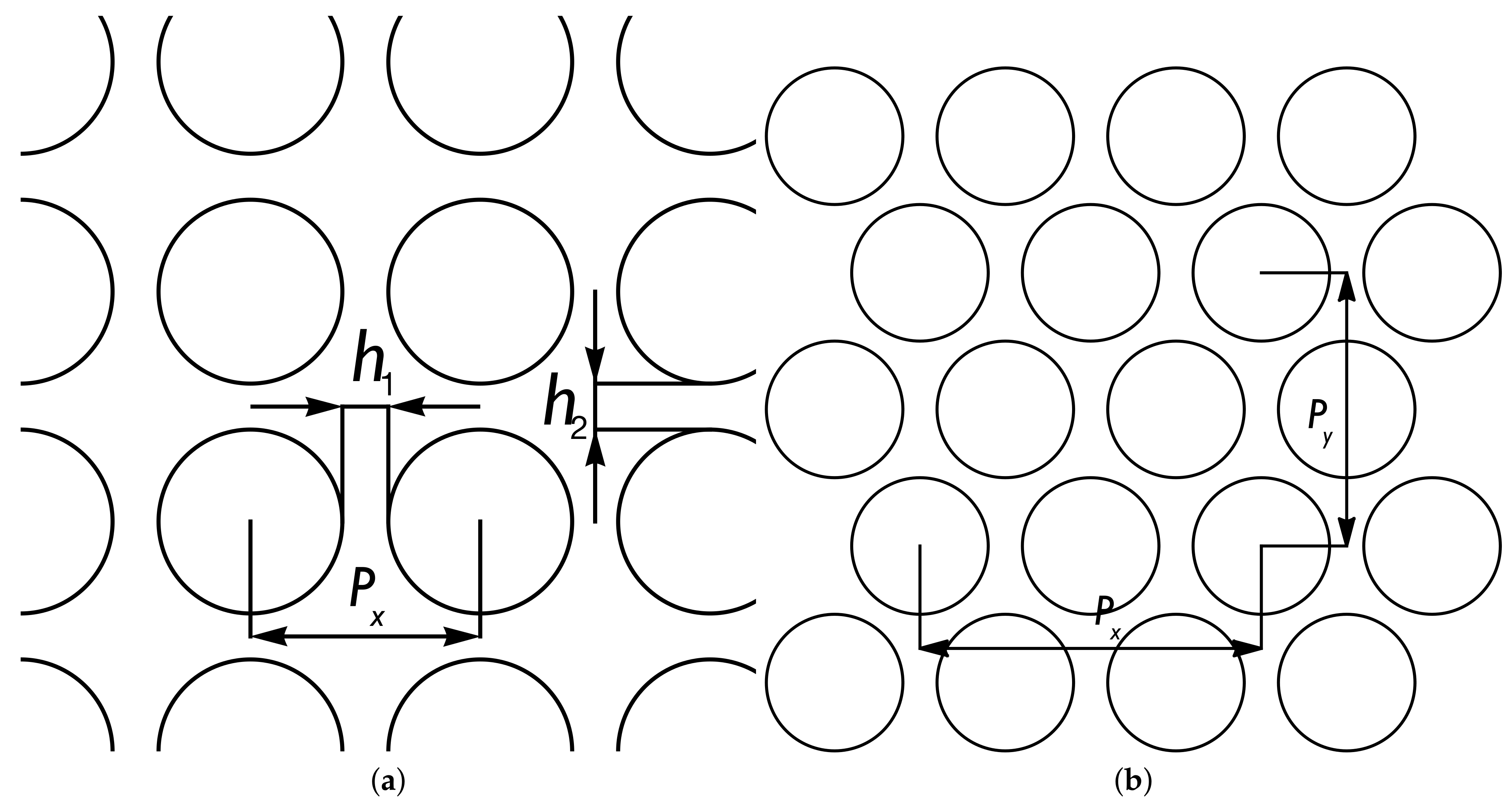
The quantity used to characterize perforated sheets of metal is the ligament efficiency . Let us assume that the holes are ellipses with a, b as the horizontal and perpendicular semiaxis, and the separation of the centers used in the definitions is and , respectively. Following [17,18,19], one can define both the horizontal and perpendicular ligament efficiency, denoting them as and , respectively. For regular arrays of holes,
and for triangular arrays, allowing for alternating layers,
2.4. Finite Element Method
All numerical simulations reported here have been computed with two different high-order continuous Galerkin codes in 2D solving the variational formulation on conforming meshes of quadrilateral or triangular elements.
One of the challenges in shell problems is to avoid numerical locking. Instead of using special shell elements [1], one can let the higher-order FEM alleviate the locking and accept that some thickness dependent error amplification or locking factor, , is unavoidable. For the -FEM solution, one can derive a simple error formulation
where h is the mesh spacing, is the diameter of the domain, and p is the degree of the elements. It is possible that diverges as t tends to zero, with the worst case being for pure bending problems: . In (16), the latter part follows from standard approximation theory of the FEM. It is the term that is shell specific. If the bending part in the energy expressions given below dominates, the energy norm depends linearly on t and hence any energy error estimate has an inverse dependence, that is, . This simple error formula suggests why higher-order methods are advantageous in shell problems: the mesh over-refinement in the "worst" case is , which for a fixed , say, indicates that for the requirement is moderate in comparison to the case of . This also suggests that convergence in p is a useful measure if the problem is otherwise difficult to analyze exactly. For a more detailed discussion on this and further references, see [20,21].
Implementations
The first solver used in this study is implemented with Mathematica, providing exact geometry handling of the holes via blending functions [22]. The second one is AptoFEM, a parallel code implemented in FORTRAN90 and MPI. Both codes allow for arbitrary order of polynomials to be used in the elements including different orders of polynomials in individual elements in the same mesh [14].
3. Shell Models
If the shell of revolution is defined by the profile function defined over some interval , then using the derivatives of the profile function all shell geometries can be classified in terms of Gaussian curvature (see, for instance, [23]). The analysis of shell problems is greatly simplified if the type of curvature is uniform.
- 1
- Parabolic (Zero Gaussian curvature shells). .
- 2
- Elliptic (Positive Gaussian curvature shells). .
- 3
- Hyperbolic (Negative Gaussian curvature shells). .
Dimensionally Reduced Elasticity Equations: Naghdi Model
Consider a shell of (constant) thickness d, the mid-surface of which occupies a region to of some smooth surface . This is a three-dimensional body equipped with principal curvature coordinates as defined in Section 2.2 for which the 3D theory of linear elasticity could be considered "exact" for small deformations. One of the classical dimension reduction models is applied here, since these models reveal the nature of shell deformations more explicitly. Such models are often reasonably accurate for thin shells [3]. The displacement field u has five components, u, v, w, , and , each of which is a function of two variables on the mid-surface of the shell. The first two components represent the tangential displacements of the mid-surface, w is the transverse deflection, and and are dimensionless rotations. The model is similar to the Reissner–Mindlin model for plate bending and is sometimes named after Naghdi. Assume that the shell consists of homogeneous isotropic material with Young modulus E and Poisson ratio . Then, the total energy of the shell in our dimension reduction model is expressed as
where is a scaling factor, q is the external load potential, and and represent the portions of total deformation energy that are stored in membrane and transverse shear deformations and bending deformations, respectively. The latter are quadratic forms independent of d and defined as
where , , and stand for the membrane, transverse shear, and bending strains, respectively. The strain-displacement relations are linear and involve at most first derivatives of the displacement components.
Remark 1.
In the following, we shall omit the constant factor from the energy expressions. Consequently, all results can be considered to be scaled with a factor .
Following [16], the bending strains are
similarly the membrane strains
and finally the shear strains
Remark 2.
When the shell parametrisations defined above are used, all terms of the form are identically zero.
The energy norm is defined in a natural way in terms of the deformation energy and taking the scaling into account:
Similarly for bending, membrane, and shear energies:
The load potential has the form If the load acts in the transverse direction of the shell surface, i.e., , and holds, then the variational problem has a unique weak solution . The corresponding result is true in the finite dimensional case, when the finite element method is employed.
In the following discussion, both free vibration and buckling problems will be briefly covered. To this effect, the mass matrix is defined as , with (displacements) and (rotations) independent of t.
The geometric stiffness matrix used in buckling analysis in the dimensionally reduced case is still without a universally agreed definition (See Appendix B). Here, in the cylindrical case, the geometric stiffness matrix is taken to be the inner product of the axial derivative of the transverse deflection with itself as suggested in [11]. Formally,
4. Boundary and Internal Layers
The theory of one-dimensional -approximation of boundary layers is due to Schwab [24]. Boundary layer functions are of the form where is a small parameter, is a constant, and L is the characteristic length scale of the problem under consideration. Even though in certain classes of problems it is possible to choose a robust strategy leading to uniform convergence in , the distribution of the mesh nodes depends on p, and over a range of polynomial degrees , say, the mesh is different for every p. In 2D, this requires one to allow for the mesh topology to change over the range of polynomial degrees. In this study, the short-range layers have been addressed in the meshes, but optimality in p has not been attempted.
It is useful to define the central concepts in a problem-independent manner.
Definition 1
(Layer Element Width). For every boundary layer in the problem, one should have an element of width in the direction of the decay of the layer.
Note, that with c constant, if as p increases, the standard p-method can be interpreted as the limiting method. Boundary layers can also occur within the domains, i.e., be internal layers, or emanate from a point. For our discussion, it is useful to define the concept of boundary layer generators (see [3]).
Definition 2
(Layer Generator). The subset of the domain from which the boundary layer decays exponentially, is called the layer generator. Formally, the layer generator is of measure zero.
The layer generators are independent of the length scale of the problem under consideration.
The types of layers that a shell structure can exhibit depend on its geometry, that is, on local curvature. Elliptic, parabolic, and hyperbolic structures each possess a distinctive set of layer deformations. The layer structure is classically assumed to be an exponential solution to the homogeneous Euler equations of the shell problem. In [3], it is shown using the Ansatz that solutions with such that the characteristic lengths are of the form where . Here, is the coordinate orthogonal to the layer generator. From these, the layer with is present in all geometries, whereas layers with and are present only in hyperbolic and parabolic geometries, respectively. The case arises from a shear deformation and shows up only when a model similar to the model of Reissner and Naghdi is used in analysis.
If the curved generators are included [5], more characteristic lengths can be found. In particular, for elliptic shells with a parabolic curved layer generator, any can be induced. Consider a shell structure generated by a rotation around the y-axis of the profile so that at the geometry parameters will vanish, otherwise we have an elliptic shell. The solution to the shell problem under unit pressure is a layer deformation in the scale .
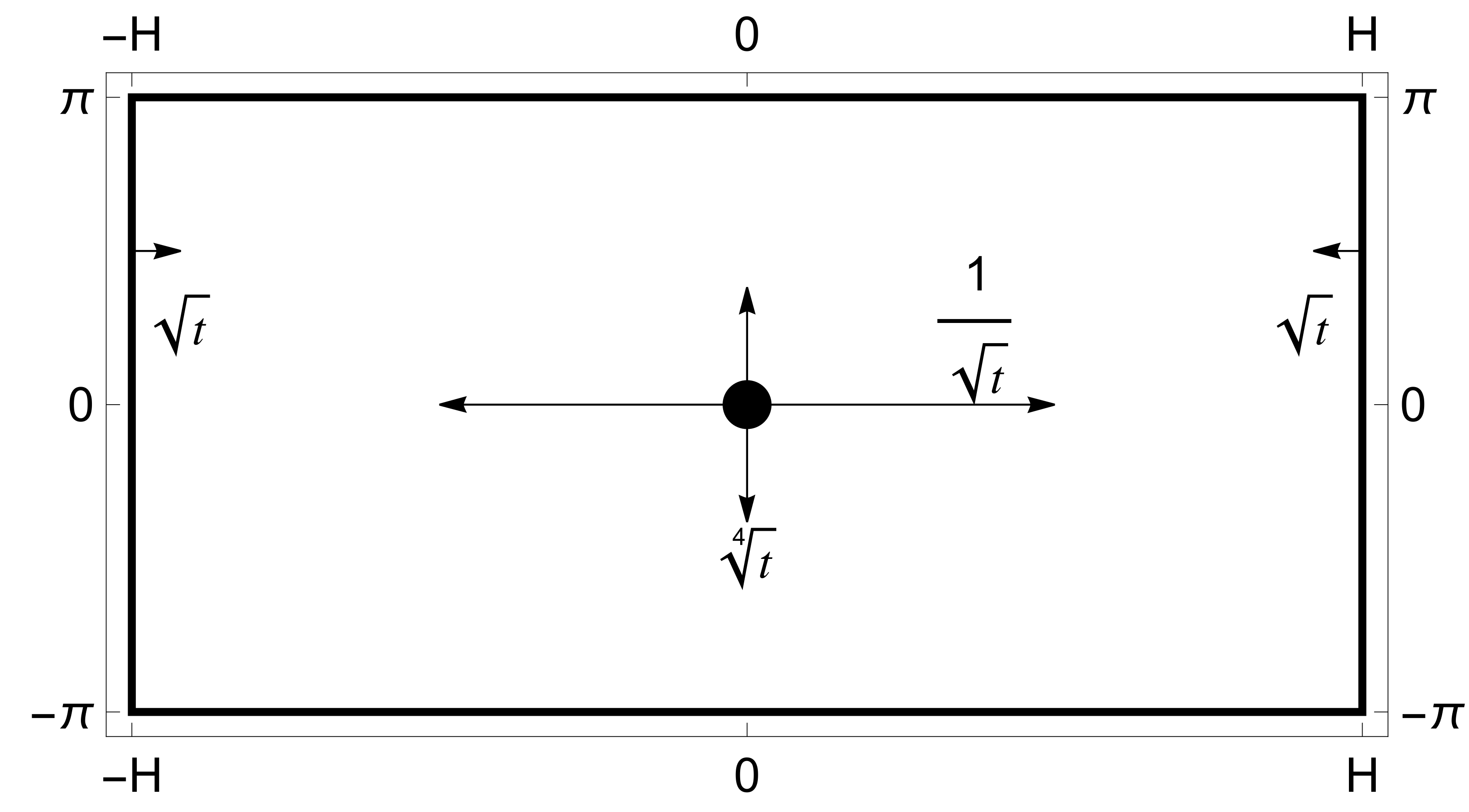
Finally, the long-range layers have the characteristic lengths and , where the first one is the axial torsion boundary layer, and the second is, for instance, induced by kinematic constraints in part of a long cylinder such a T-junction. These layers are referred to as long-range Fourier modes in Section 3.2 of [3]. The layer chart for a long cylinder is given in Figure 3.
5. Numerical Simulations
The three simulation sets considered here have been tabulated in Table 1. They have been selected to illustrate each of the three main types of long-range layers including perforated variants. The relative effects of the perforations on the fundamental natural frequency are given as ratios of the perforated and reference frequencies. For every realization of the shell geometry, five logarithmically equidistant thicknesses have been used. All parabolic cases have been computed using both Naghdi and shallow shell models and as expected, the differences are negligible. The hyperbolic and elliptic cases have been simulated with the Naghdi model only. In all cases where short-range layers have been present at the clamped boundaries, the meshes have been adapted a priori to the corresponding length scales. In all structures with perforation patterns, the holes are free; that is, there are no kinematical constraints.
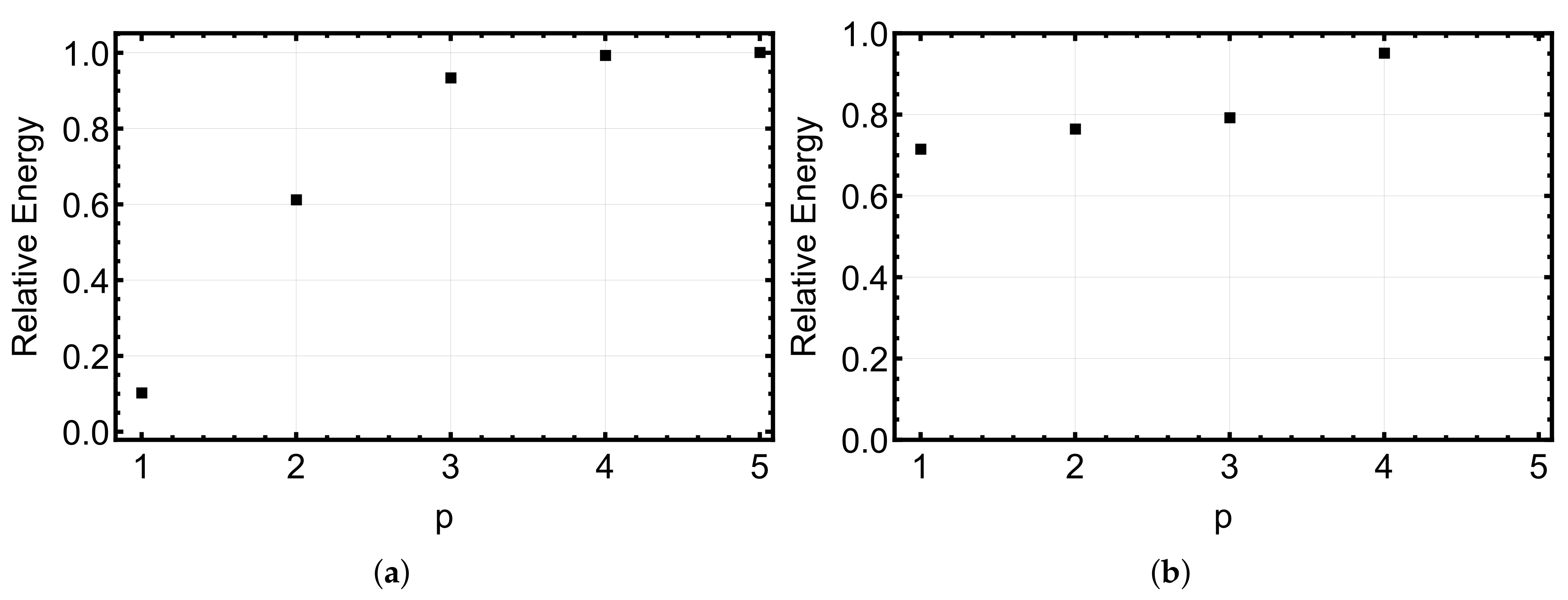
The selected polynomial orders can be justified by considering the energy convergence in p. In Figure 4, two examples of convergence graphs are shown.
5.1. Wind Turbine: Manhole
The first simulation concerns the long-range layer on long or tall structures with a kinematically constrained section within the domain. The manhole title is inspired by an example in [8], (Figure 1). The authors discuss the effects of various stiffeners for the manhole of a wind tower. In their FEM analysis figure, the long-range effect is clearly visible but not shown at full length. The construction reported has a dimensional thickness of , so it falls within the realm of thin structures.
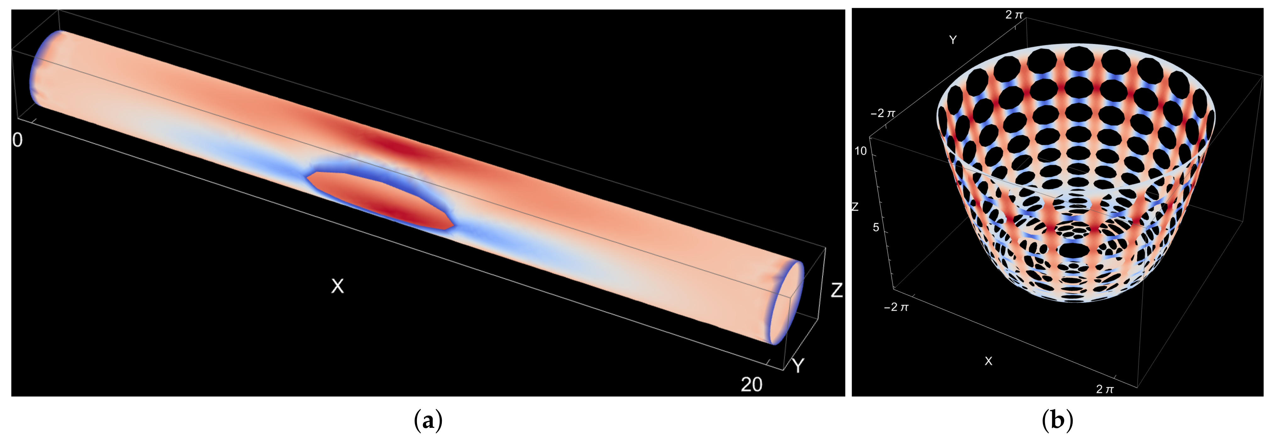
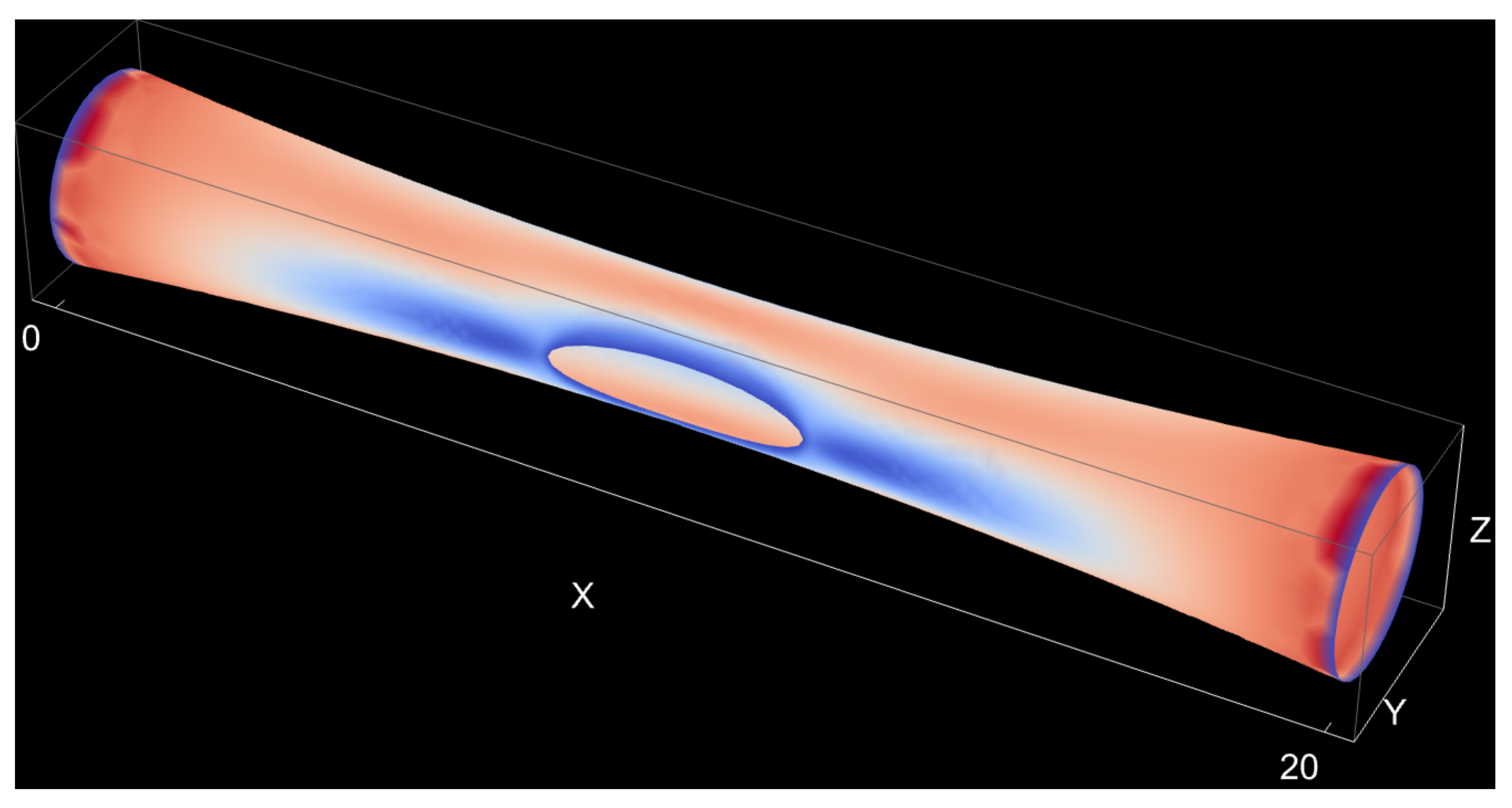
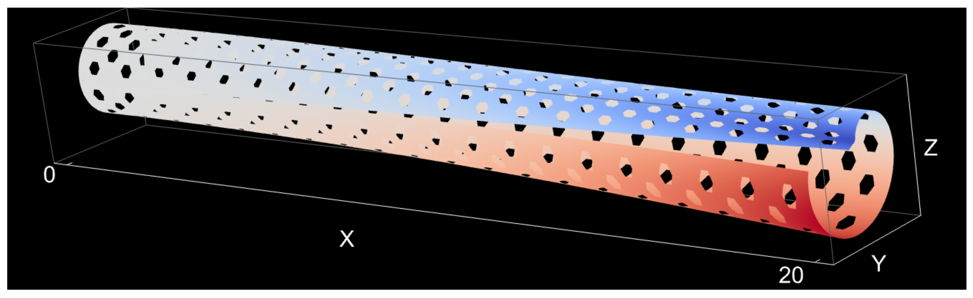
In Figure 1a and Figure 5, the overall solutions are shown for parabolic and hyperbolic shells, respectively. The overall features predicted in the layer chart of Figure 3 are clearly visible in both cases. The effect of the length H of the structure is shown in Figure 6. The long-range extends further in the longer cylinder as expected, since , whereas .
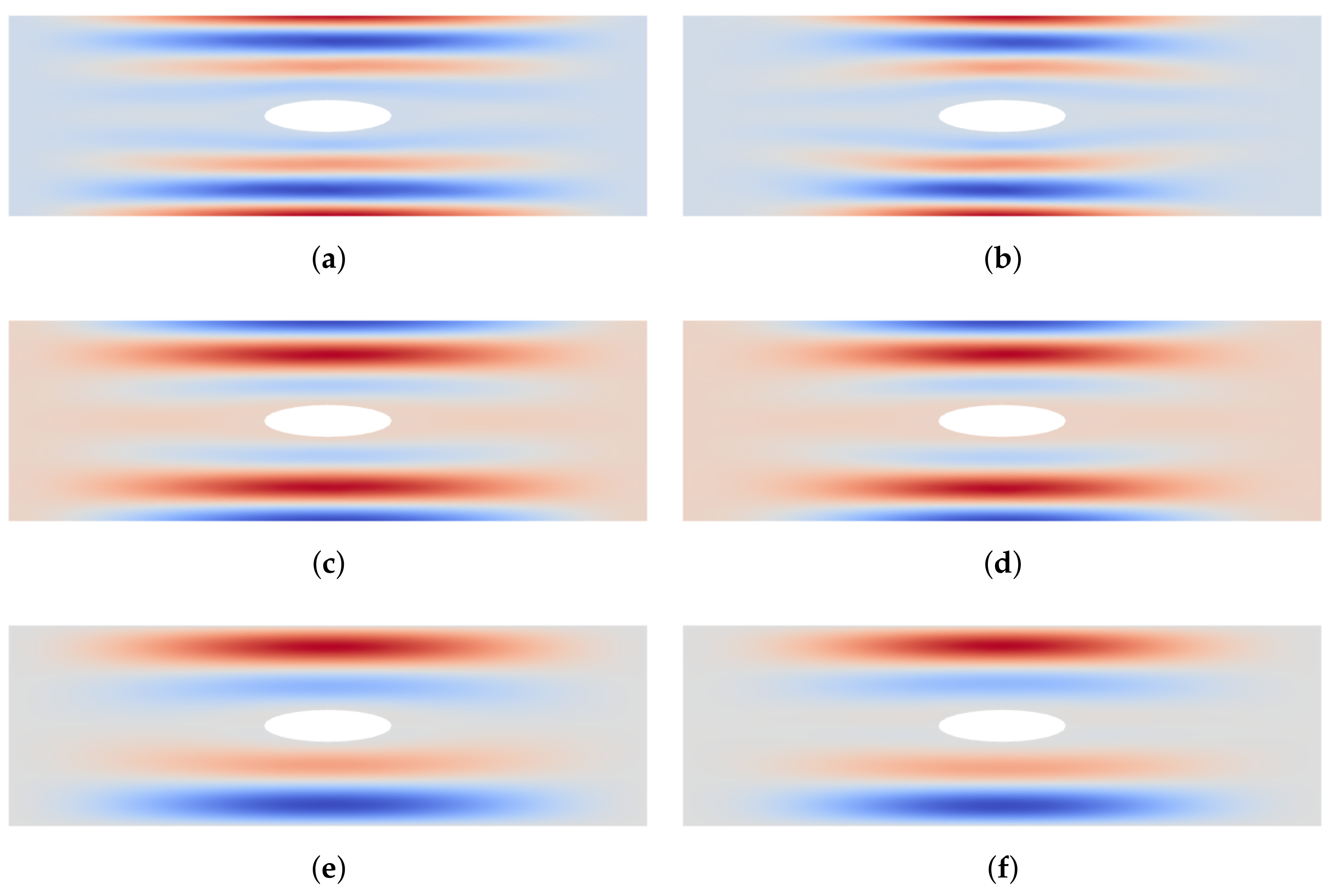
The asymptotic behavior of the eigenmodes in the free vibration of shells of revolution is known [25]. It is of interest to monitor the effect of the hole to the lowest eigenvalue. Transverse profiles are shown in Figure 7. Since the hyperbolic profile is only mildly hyperbolic and the interval of thicknesses is kept realistic, the profiles appear very similar with the oscillations only slightly more concentrated in the center in the hyperbolic case. Assuming the same material parameters, the eigenvalue amplification due to the hole is smaller in the hyperbolic case. In both cases, the amplification decreases as . This is due to angular oscillations (wave numbers) increasing as and hence the interaction of the hole and the layers becomes weaker.
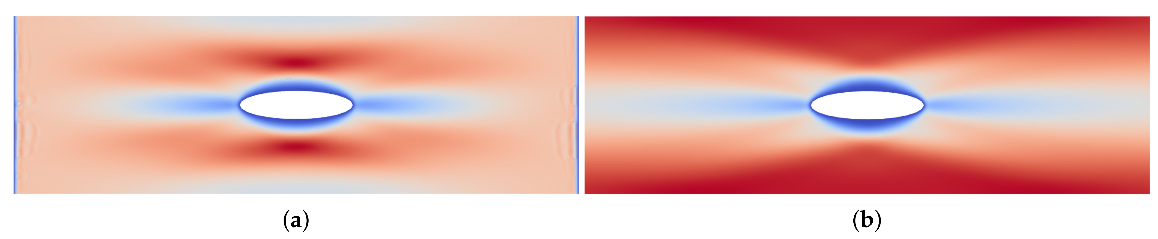
Of course, for cylindrical or parabolic shells, there is also the relative long layer of in the angular dimension. In Figure 8, this effect is shown by visual comparison of two profiles corresponding to different thicknesses. Since the eigenmodes oscillate in the angular direction as seen in Figure 7, the effect of the hole is very small in the eigenvalues, with the increase in the ratio less than 1%.
Remark 3.
For hyperbolic shells, the layer does not exist. Instead, there is a layer along the characteristics of the surface. In Figure 5, the shell is nearly parabolic in the vicinity of the hole and therefore this feature is not visible.
Confirming the correct length scales is difficult since the long-range effects do not occur in isolation, but in all cases the deflection profile is a linear combination of different characteristic features. Using interpolated representations, the long-range effect is associated with the inflection point of the curve. The two thinnest cases are used to estimate the constant of the layer, and this value is used to predict the corresponding locations in the other cases.
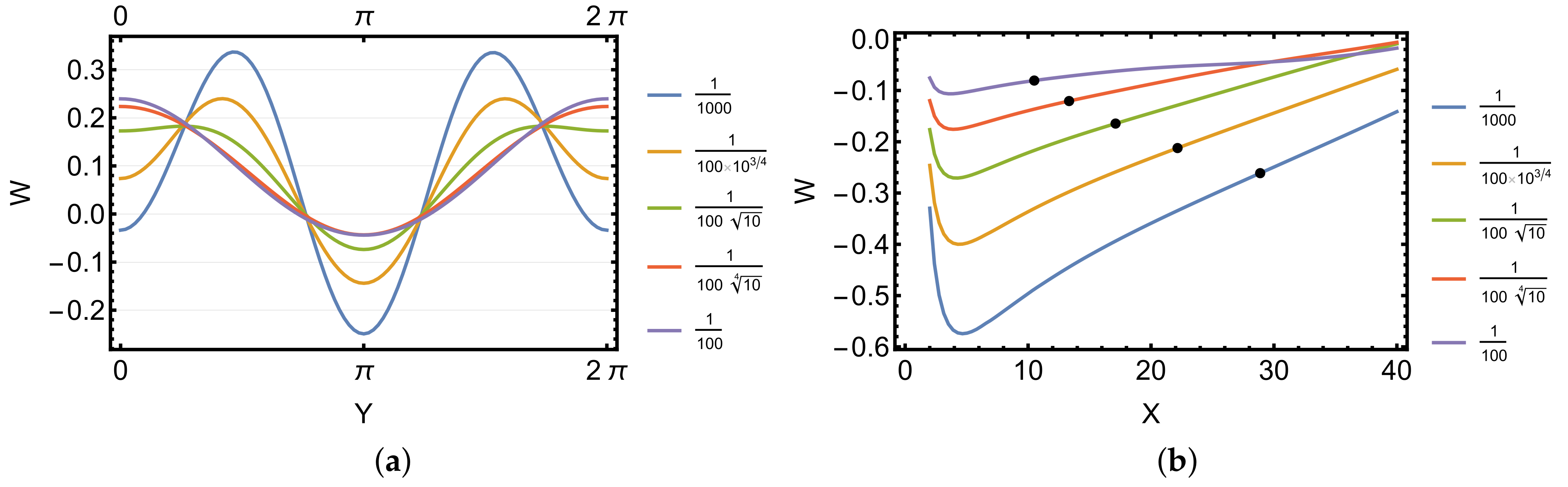
In Figure 9a, another view to the angular layers is given. In addition, in Figure 9b, the agreement with the predicted length scale is illustrated. However, it appears that the clamped end at already affects the overall profile. The estimated constant is leading to model . In Figure 10, two long configurations with different geometries have been considered. The displacement graphs over a set of thicknesses show the stronger short-range effects. As can be seen, in the longer cases, , the agreement is very good indeed. Notice that the good agreement is on the axial rotation component , which means that domain expertise has been necessary to find the right component.
5.2. Slit Shells: Torsion Effect
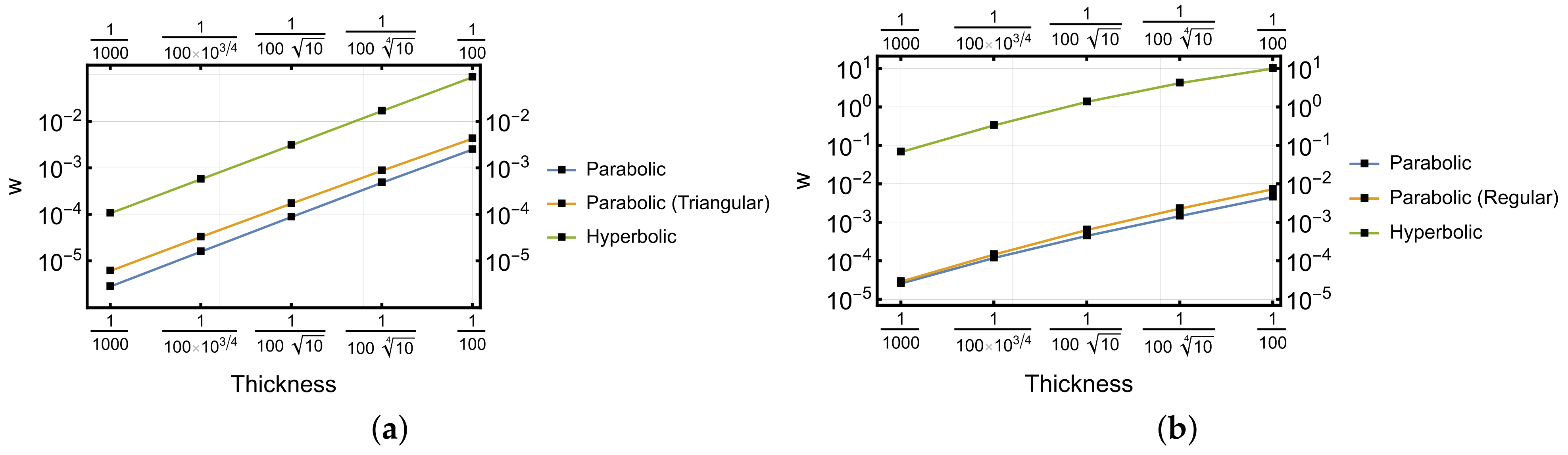
The torsion layer is naturally the most difficult to recover from simulation data. The effect on a slit cylinder is illustrated in Figure 11. The boundary at is clamped, , but all other boundaries are free. The loading is a unit torsion load acting on the boundary at . The technique used in the previous case was not successful here. Indeed, the exact layer could not be found from the data. However, the effect of H can be deduced indirectly by observing the rate of change of curvature of the displacement profile over a set of thicknesses after the loading is scaled by . In Figure 12a, for the slopes for both geometries, including a parabolic perforated case, the trends are constant. In Figure 12b, for the observed trends are somewhat polluted, but the important aspect for this discussion is that as the shell becomes longer, and the torsion effect becomes milder indicating the presence of a long-range layer. Since this phenomenon also exists at for , it is likely that it is due to the corresponding predicted layer.
Interestingly, the first eigenmode corresponds to the kind of rotation caused by the chosen loading in the static case, and therefore the figure has been omitted. Now, the perforated case is softer (the holes are free), and hence the ratios are less than one, and decreasing as . For , the ratio is 0.64, whereas for , it is 0.42.
5.3. Curvature Effect
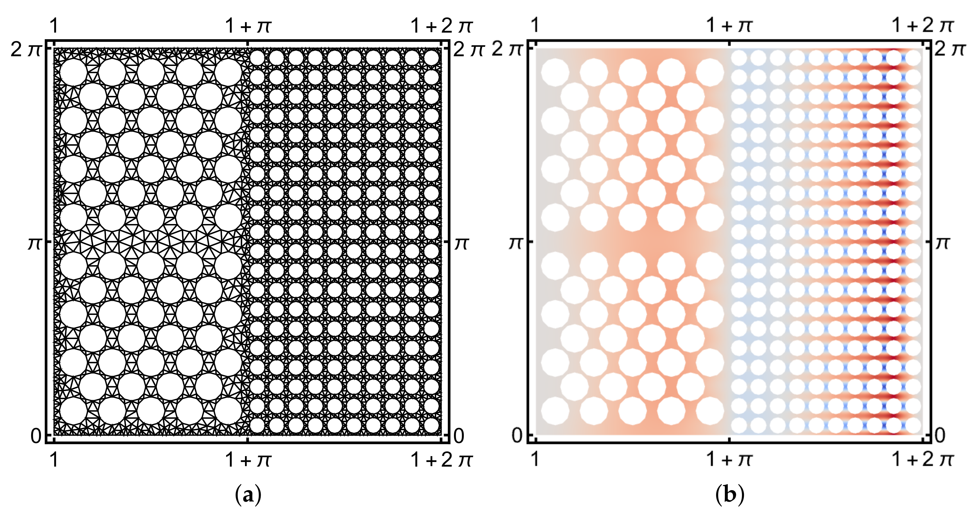
The third and final simulation adds two aspects: First, the layer generator is curved, and second, the shell geometry is not of uniform type. The shell of revolution is formed by letting a profile function , , and , . In other words, the inner section is a plate and the outer section is an elliptic extension with curvature dependent on . One realization is shown in Figure 1b. The parameter determines the length of the layer. Two sets of simulations with or are computed on the multipanel mesh of Figure 13a. The inner holes are free and therefore as increases and for a fixed loading, the displacement amplitudes increase due to the sensitivity of the problem. However, for a given range of thicknesses, the response of the structure is reasonable (see Figure 13b).
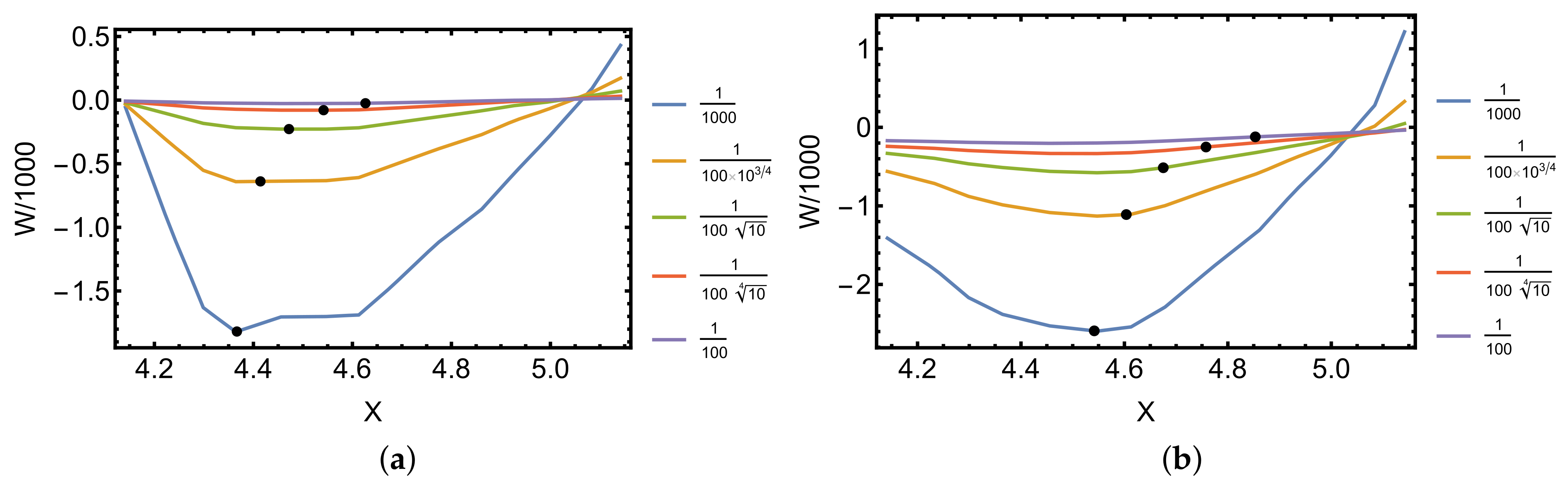
For small values of the recovery of the length scales is successful (see Figure 14). In the previous study on curved generators, the plate was not present, and the structure was not perforated. This clearly indicates that these effects are features of the elasticity equations irrespective of the effective material properties.
The eigenanalysis becomes more involved in this case. As can be seen in Figure 15, the (relative) transverse deflection profiles are almost dramatically different. This is due to the free holes in the elliptic part exhibiting sensitivity [6]. The eigenmode includes strong oscillations in the elliptic part, a phenomenon that does not have any corresponding effect in the reference case where the oscillation is confined to the plate section. It is due to sensitivity that the eigenvalues ratios increase as . For , the ratio is 0.26, whereas for , it is 0.48.
6. Conclusions
Shell structures have a rich family of boundary layers including internal layers. Each layer has its own characteristic length scale, which depends on the thickness of the shell. The long-range layers do exist, and in certain problem classes play an important role. Interestingly, since they are not well-known, it is possible that in some problems new modeling ideas might be brought forward if only they were recognized in the right contexts.
The simulation of such structures is subject to numerical locking, and high-order finite element methods provide one way to derive reliable solutions. The observed asymptotic behavior is consistent with the theoretical predictions. These layers are shown to also appear on perforated structures underlying the fact these features are properties of the elasticity equations and not dependent on the effective materials.
Funding
This research received no external funding.
Data Availability Statement
Not applicable.
Acknowledgments
I would like to thank the anonymous referees for suggestions that improved the paper considerably.
Conflicts of Interest
The author declares no conflict of interest.
Appendix A. Mathematical Shell Model
In the following, the Naghdi model is simplified by assuming that is a domain expressed in the coordinates x and y. The curvature tensor of the midsurface is assumed to be constant and , and . The shell is then called elliptic when , parabolic when , and hyperbolic when . The above assumptions are valid when the shell is shallow, i.e., the midsurface differs only slightly from a plane. In the simplest case, one may set and write the relation between the strain and the displacement fields as
This choice of shell model gives us additional flexibility in the design of the numerical simulations since the model admits non-realizable shell geometries. This is due to the assumption that the local curvatures are constant at every point of the surface.
Remarkably, for parabolic shells these strains differ from those of the standard Naghdi model only in and , when the radius is . Naturally, for non-parabolic geometries the differences are much more extensive. Notice that the resulting system has constant coefficients, which simplifies the implementation of the model significantly.
Appendix B. On Buckling Modes
The critical load of the real shell is known to be very sensitive to small geometric imperfections and deviations in boundary conditions, which are difficult to take into account in linear or nonlinear stability theory. As a result, theoretical and experimental results do not agree well in many loading scenarios. In any case, the linear stability theory provides useful information regarding the buckling behavior of thin shells [11].
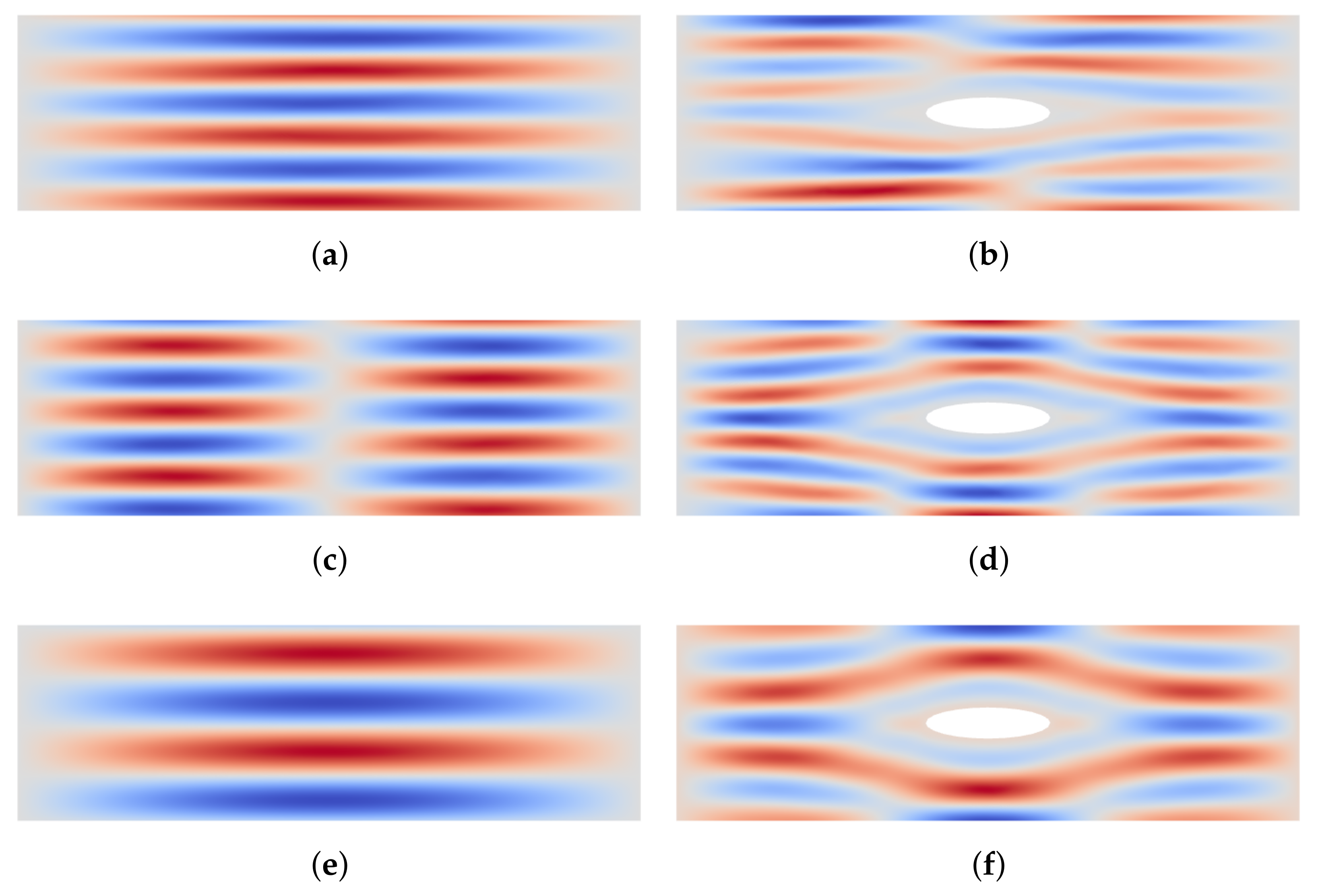
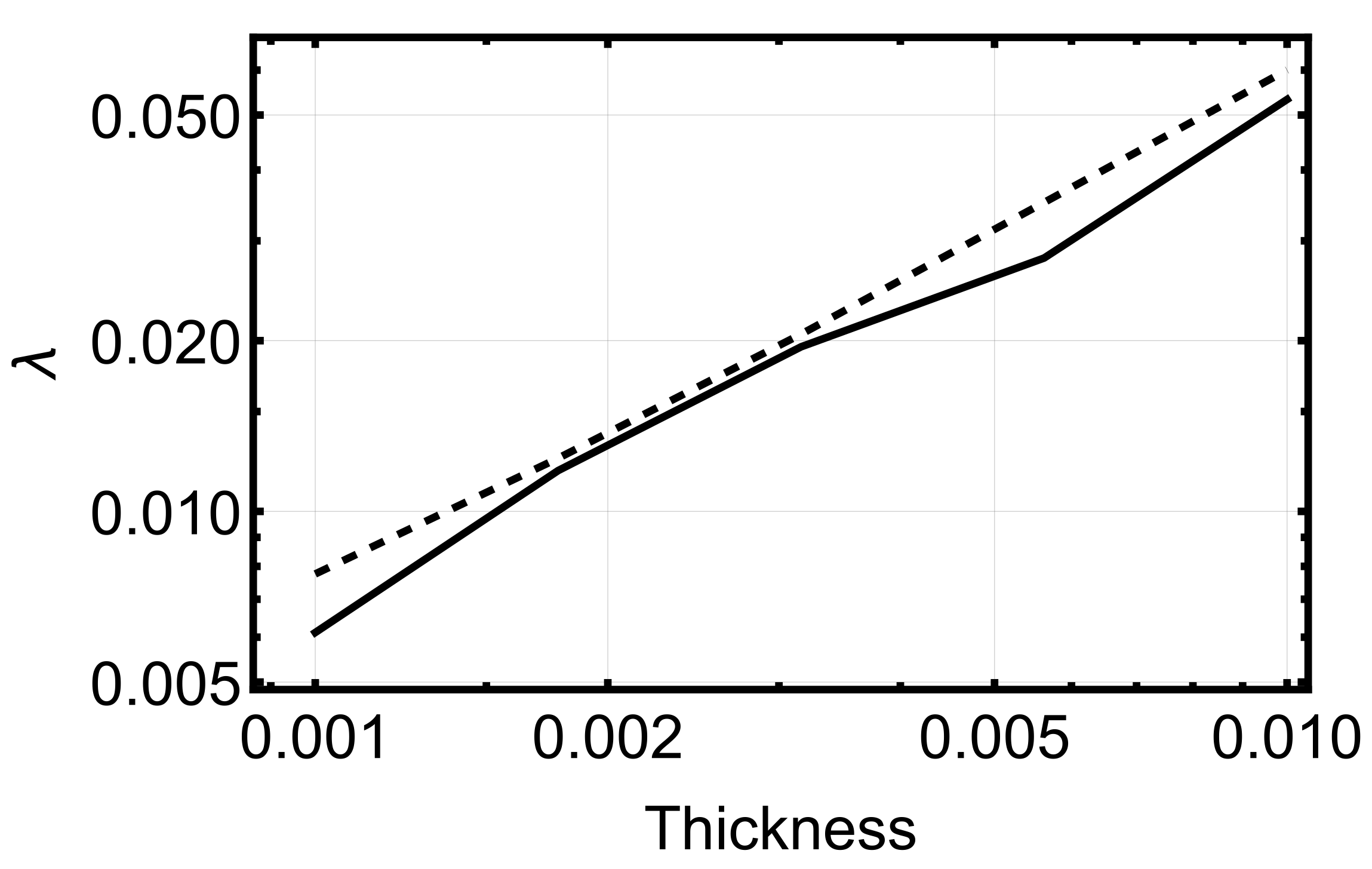
The first buckling modes are shown in Figure A1. Interestingly, even in the reference case, the lowest mode can exhibit axial oscillations. In the profile of the thinnest configuration with a hole, symmetry appears to be lost. This is due to the extreme ill-conditioning of the problem. Also in contrast with the free vibration, here the eigenvalue ratio between the perforated and reference configurations does not change as (see Figure A2). In both cases, the dependence is linear, which is in fact a new result. It should be noted that in simulations with the given buckling model, the observed spectrum is clustered for every fixed thickness. For instance, the relative difference within the first ten modes is less than 1% in the case with a hole, and a fraction higher in the reference case. In fact, it has been proposed that the Shapiro–Lopatinsky conditions are not satisfied in the limit and the coercivity is lost, just as for the sensitive elliptic shells [6].
Figure A1.
Buckling modes: Transverse deflection profiles of first modes. In both cases, , the hole is kinematically fully constrained, , and the ends have . From top: . (a,c,e) Parabolic reference. (b,d,f) Parabolic with a hole.
Figure A1.
Buckling modes: Transverse deflection profiles of first modes. In both cases, , the hole is kinematically fully constrained, , and the ends have . From top: . (a,c,e) Parabolic reference. (b,d,f) Parabolic with a hole.

Figure A2.
Buckling modes: Linear dependence of the observed smallest (eigenvalue corresponding to the critical load) to the thickness. Thick line: Reference. Dashed line: With hole.
Figure A2.
Buckling modes: Linear dependence of the observed smallest (eigenvalue corresponding to the critical load) to the thickness. Thick line: Reference. Dashed line: With hole.

This set of simulations simply illustrates the inherent complexity of the buckling problem in this context. Many fundamental concepts remain open starting from the selection of the right model and kinematic constraints.
References
- Chapelle, D.; Bathe, K.J. The Finite Element Analysis of Shells; Springer: Berlin/Heidelberg, Germany, 2003. [Google Scholar]
- Pitkäranta, J.; Leino, Y.; Ovaskainen, O.; Piila, J. Shell Deformation states and the Finite Element Method: A Benchmark Study of Cylindrical Shells. Comput. Methods Appl. Mech. Eng. 1995, 128, 81–121. [Google Scholar] [CrossRef]
- Pitkäranta, J.; Matache, A.M.; Schwab, C. Fourier mode analysis of layers in shallow shell deformations. Comput. Methods Appl. Mech. Eng. 2001, 190, 2943–2975. [Google Scholar] [CrossRef] [Green Version]
- Hakula, H.; Havu, V.; Beirao de Veiga, L. Long-Range Boundary Layers in Shells of Revolution. In Proceedings of the 5th International Conference on Computation of Shell and Spatial Structures, Salzburg, Austria, 1–4 June 2005. [Google Scholar]
- Hakula, H. Hp-boundary layer mesh sequences with applications to shell problems. Comput. Math. Appl. 2014, 67, 899–917. [Google Scholar] [CrossRef]
- Sanchez-Palencia, E.; Millet, O.; Béchet, F. Singular Problems in Shell Theory; Springer: Berlin/Heidelberg, Germany, 2010. [Google Scholar]
- Pietraszkiewicz, W.; Konopińska, V. Junctions in shell structures: A review. Thin Walled Struct. 2015, 95, 310–334. [Google Scholar] [CrossRef]
- Malliotakis, G.; Alevras, P.; Baniotopoulos, C. Recent Advances in Vibration Control Methods for Wind Turbine Towers. Energies 2021, 14, 7536. [Google Scholar] [CrossRef]
- Szabo, B.A.; Muntges, D.E. Procedures for the Verification and Validation of Working Models for Structural Shells. J. Appl. Mech. 2005, 72, 907–915. [Google Scholar] [CrossRef]
- Szabo, B.; Babuska, I. Finite Element Analysis; Wiley: Hoboken, NJ, USA, 1991. [Google Scholar]
- Niemi, A.H. Numerical buckling analysis of circular cylindrical shells. In Proceedings of the MAFELAP 2019, Uxbridge, UK, 18–21 June 2019. [Google Scholar]
- Bartels, S.; Bonito, A.; Muliana, A.H.; Nochetto, R.H. Modeling and simulation of thermally actuated bilayer plates. J. Comput. Phys. 2018, 354, 512–528. [Google Scholar] [CrossRef] [Green Version]
- McMillen, T.; Goriely, A. Tendril Perversion in Intrinsically Curved Rods. J. Nonlinear Sci. 2002, 12, 241–281. [Google Scholar] [CrossRef]
- Giani, S.; Hakula, H. On effective material parameters of thin perforated shells under static loading. Comput. Methods Appl. Mech. Eng. 2020, 367, 113094. [Google Scholar] [CrossRef]
- Slaughter, W.S. The Linearized Theory of Elasticity; Birkhäuser: Basel, Switzerland, 2002. [Google Scholar]
- Malinen, M. On the classical shell model underlying bilinear degenerated shell finite elements: General shell geometry. Int. J. Numer. Methods Eng. 2002, 55, 629–652. [Google Scholar] [CrossRef]
- Forskitt, M.; Moon, J.R.; Brook, P.A. Elastic properties of plates perforated by elliptical holes. Appl. Math. Model. 1991, 15, 182–190. [Google Scholar] [CrossRef]
- Burgemeister, K.; Hansen, C. Calculating Resonance Frequencies of Perforated Panels. J. Sound Vib. 1996, 196, 387–399. [Google Scholar] [CrossRef]
- Jhung, M.J.; Yu, S.O. Study on modal characteristics of perforated shell using effective Young’s modulus. Nucl. Eng. Des. 2011, 241, 2026–2033. [Google Scholar] [CrossRef]
- Pitkäranta, J. The problem of membrane locking in finite element analysis of cylindrical shells. Numer. Math. 1992, 61, 523–542. [Google Scholar] [CrossRef]
- Hakula, H.; Leino, Y.; Pitkäranta, J. Scale resolution, locking, and high-order finite element modelling of shells. Comput. Methods Appl. Mech. Engrg. 1996, 133, 157–182. [Google Scholar] [CrossRef]
- Hakula, H.; Tuominen, T. Mathematica implementation of the high order finite element method applied to eigenproblems. Computing 2013, 95, 277–301. [Google Scholar] [CrossRef]
- Do Carmo, M. Differential Geometry of Curves and Surfaces; Prentice Hall: Hoboken, NJ, USA, 1976. [Google Scholar]
- Schwab, C. p- and hp-Finite Element Methods; Oxford University Press: Oxford, UK, 1998. [Google Scholar]
- Artioli, E.; da Veiga, L.B.; Hakula, H.; Lovadina, C. On the asymptotic behaviour of shells of revolution in free vibration. Comput. Mech. 2009, 44, 45–60. [Google Scholar] [CrossRef]
Figure 1.
Examples of structures subject to long-range layers: transverse deflection profiles. In both cases, the dimensionless thickness , all boundaries are kinematically fully constrained, and the loading is the unit pressure. (a): Long cylinder with an ellipsoidal hole. (b): Circular plate with an elliptic extension. The load is acting only on the extension.

Figure 2.
Penetration patterns. (a) Regular pattern. (b) Triangular pattern.

Figure 3.
Layer structure: Parabolic long cylinder. The expected length scales are indicated with the arrows. The generators are the boundaries at , and the hole in the center. The location of the center does not play a role. If the periodic boundary at is free, under torsion there will be a very long layer . The hole also generates a short range axial layer, which is not indicated.

Figure 4.
Numerical Locking: p-convergence in energy. Total energy at is taken as the reference. (a) Circular plate with an elliptic extension under unit pressure on the extension. (b) Long slit parabolic cylinder with a regular perforation pattern under torsion loading. In both cases starting at , the relative error in energy is sufficiently small, justifying the selected polynomial orders.

Figure 5.
Long hyperbolic shell with an ellipsoidal hole. Transverse deflection profile when the dimensionless thickness , all boundaries are kinematically fully constrained, , and the loading is the unit pressure.
Figure 5.
Long hyperbolic shell with an ellipsoidal hole. Transverse deflection profile when the dimensionless thickness , all boundaries are kinematically fully constrained, , and the loading is the unit pressure.

Figure 6.
Two long cylinders: Transverse deflection profiles. In both cases, the dimensionless thickness , all boundaries are kinematically fully constrained, , and the loading is the unit pressure. (a) . (b) , with the centre section shown.
Figure 6.
Two long cylinders: Transverse deflection profiles. In both cases, the dimensionless thickness , all boundaries are kinematically fully constrained, , and the loading is the unit pressure. (a) . (b) , with the centre section shown.

Figure 7.
Free vibration: Transverse deflection profiles of first eigenmodes. In both cases, and all boundaries are kinematically fully constrained, . From top: . Ratio of the observed eigenvalue over the reference eigenvalues: (a,c,e) (Parabolic) – . (b,d,f) (Hyperbolic) – .
Figure 7.
Free vibration: Transverse deflection profiles of first eigenmodes. In both cases, and all boundaries are kinematically fully constrained, . From top: . Ratio of the observed eigenvalue over the reference eigenvalues: (a,c,e) (Parabolic) – . (b,d,f) (Hyperbolic) – .

Figure 8.
Manhole: Transverse deflection profiles. In both cases, , boundaries are kinematically fully constrained, , and the loading is the unit pressure. (a) , . (b) , .
Figure 8.
Manhole: Transverse deflection profiles. In both cases, , boundaries are kinematically fully constrained, , and the loading is the unit pressure. (a) , . (b) , .

Figure 9.
Manhole: Transverse deflection profiles and predicted characteristic length scales. Case with ellipsoidal hole at : (a) Profiles at . (b) Observed characteristic length scales.
Figure 9.
Manhole: Transverse deflection profiles and predicted characteristic length scales. Case with ellipsoidal hole at : (a) Profiles at . (b) Observed characteristic length scales.

Figure 10.
Long-range layers: Predicted characteristic length scales. In all cases, the inflection points have been computed for the two thinnest cases and the constant has been set with these points. The constants are from left to right: , leading to models , . The rest of the points have been selected based on the theoretical prediction. The agreement is surprisingly good. (a) Parabolic case, center hole, , -component. (b) Hyperbolic case, center hole, , -component.

Figure 11.
Slit cylinder: Transverse deflection profile. Perforation pattern is triangular with hole coverage of 25%.
Figure 11.
Slit cylinder: Transverse deflection profile. Perforation pattern is triangular with hole coverage of 25%.

Figure 12.
Slit shell of revolution: Effect of the length of the shell on torsion loading acting on the free end. Parabolic and hyperbolic cases, with a perforated parabolic one as the third option. The torsion layer leads to smaller effect close to the fixed boundary. Shown is the observed transverse deflection at along the midline of the surface. (a) . The slope of the loglog-graphs is =3. (b) . The slope of the loglog-graphs is =2.

Figure 13.
Circular plate with an elliptic extension. Pressure load is acting on the right-hand-side half of the domain. The boundaries at and are clamped, , the and boundaries are periodic. The inner circular hole has a radius = 1. (a) Multipanel mesh. (b) Quadratic extension, w-component (transverse deflection), .

Figure 14.
Circular plate with an elliptic extension. Profiles along . As above, in all cases the inflection points have been computed for the two thinnest cases and the constant has been set with these points. The constant is the same in both cases: , leading to model . The rest of the points have been selected based on the theoretical prediction. Again, the agreement is very good indeed. (a) Quadratic extension, w-component (transverse deflection). (b) Cubic extension, w-component (transverse deflection).

Figure 15.
Circular plate with an elliptic extension. First eigenmodes at . The boundaries at and are clamped, the and boundaries are periodic. The inner circular hole has a radius = 1. (a) Reference domain. (b) Perforated domain, w-component (transverse deflection).
Figure 15.
Circular plate with an elliptic extension. First eigenmodes at . The boundaries at and are clamped, the and boundaries are periodic. The inner circular hole has a radius = 1. (a) Reference domain. (b) Perforated domain, w-component (transverse deflection).


Table 1.
The set of simulations with key parameters. The profile functions for the parabolic and hyperbolic cases are and , respectively. For every individual simulation, five logarithmically equidistant thicknesses have been used. H is the half-width, p the uniform polynomial order, and N is the total number of degrees of freedom. In the non-perforated Slit Shell simulations, the meshes are topologically equivalent. In the perforated cases, the hole coverage percentage is 25%, the triangular pattern is resulting in 3791 holes, and the regular pattern is resulting in 10,000 holes.
| Case | Geometry | Perforation | H | p | N |
|---|---|---|---|---|---|
| Wind Turbine: Manhole | Parabolic | 60 | 8 | 197,440 | |
| Parabolic | 1000 | 6 | 2,127,240 | ||
| Hyperbolic | 1000 | 6 | 2,127,240 | ||
| Slit Shell: Torsion Effect | Parabolic | 100 | 5 | 1,907,980 | |
| Parabolic | Triangular | 100 | 5 | 2,841,675 | |
| Hyperbolic | 100 | 5 | 1,907,980 | ||
| Parabolic | 1000 | 5 | 1,907,980 | ||
| Parabolic | Regular | 1000 | 5 | 7,126,755 | |
| Hyperbolic | 1000 | 5 | 1,907,980 | ||
| Curvature Effect | Mixed | Multipanel | 6 | 490,145 |
Disclaimer/Publisher’s Note: The statements, opinions and data contained in all publications are solely those of the individual author(s) and contributor(s) and not of MDPI and/or the editor(s). MDPI and/or the editor(s) disclaim responsibility for any injury to people or property resulting from any ideas, methods, instructions or products referred to in the content. |
© 2023 by the author. Licensee MDPI, Basel, Switzerland. This article is an open access article distributed under the terms and conditions of the Creative Commons Attribution (CC BY) license (https://creativecommons.org/licenses/by/4.0/).
Share and Cite
MDPI and ACS Style
Hakula, H. On Long-Range Characteristic Length Scales of Shell Structures. Eng 2023, 4, 884-902. https://doi.org/10.3390/eng4010053
AMA Style
Hakula H. On Long-Range Characteristic Length Scales of Shell Structures. Eng. 2023; 4(1):884-902. https://doi.org/10.3390/eng4010053
Chicago/Turabian StyleHakula, Harri. 2023. "On Long-Range Characteristic Length Scales of Shell Structures" Eng 4, no. 1: 884-902. https://doi.org/10.3390/eng4010053