
Bending and Torsional Stress Factors in Hypotrochoidal H-Profiled Shafts Standardised According to DIN 3689-1
Department of Mechanical and Automotive Engineering, Institute for Machin Development, Westsächsische Hochschule Zwickau, D-08056 Zwickau, Germany
Eng 2023, 4(1), 829-842; https://doi.org/10.3390/eng4010050
Submission received: 14 December 2022
/
Revised: 8 February 2023
/
Accepted: 1 March 2023
/
Published: 6 March 2023
(This article belongs to the Special Issue Feature Papers in Eng 2022)
Abstract
:Hypotrochoidal profile contours have been produced in industrial applications in recent years using two-spindle processes, and they are considered effective high-quality solutions for form-fit shaft and hub connections. This study mainly concerns analytical approaches to determine the stresses and deformations in hypotrochoidal profile shafts due to pure bending loads. The formulation was developed according to bending principles using the mathematical theory of elasticity and conformal mappings. The loading was further used to investigate the rotating bending behaviour. The stress factors for the classical calculation of maximum bending stresses were also determined for all those profiles presented and compiled in the German standard DIN3689-1 for practical applications. The results were also compared with the corresponding numerical and experimental results, and very good agreement was observed. Additionally, based on previous work, the stress factor was determined for the case of torsional loading to calculate the maximum torsional stresses in the standardised profiles, and the results are listed in a table. This study contributes to the further refinement of the current DIN3689 standard.
1. Introduction
In the field of modern drive technology, there is an increasing demand for higher power transmission in a smaller construction space. A necessary and important component in drive trains is the form-fit shaft and hub connections. Thereby, a widely used standard solution is the key-fit connection according to DIN 6885 [1]. However, this technique is reaching its mechanical limitations, which is why industry focus has been increasingly on form-fit connections with polygon profiles in the past few years. With the hypotrochoidal polygonal connection (H-profiles in Figure 1), a polygonal contour has been the new standard according to DIN 3689-1 [2] since November 2021. The great advantages of H-profiles via key-fit connections were studied in [3]. These investigations display a significant reduction of around 50% in the fatigue notch factor.
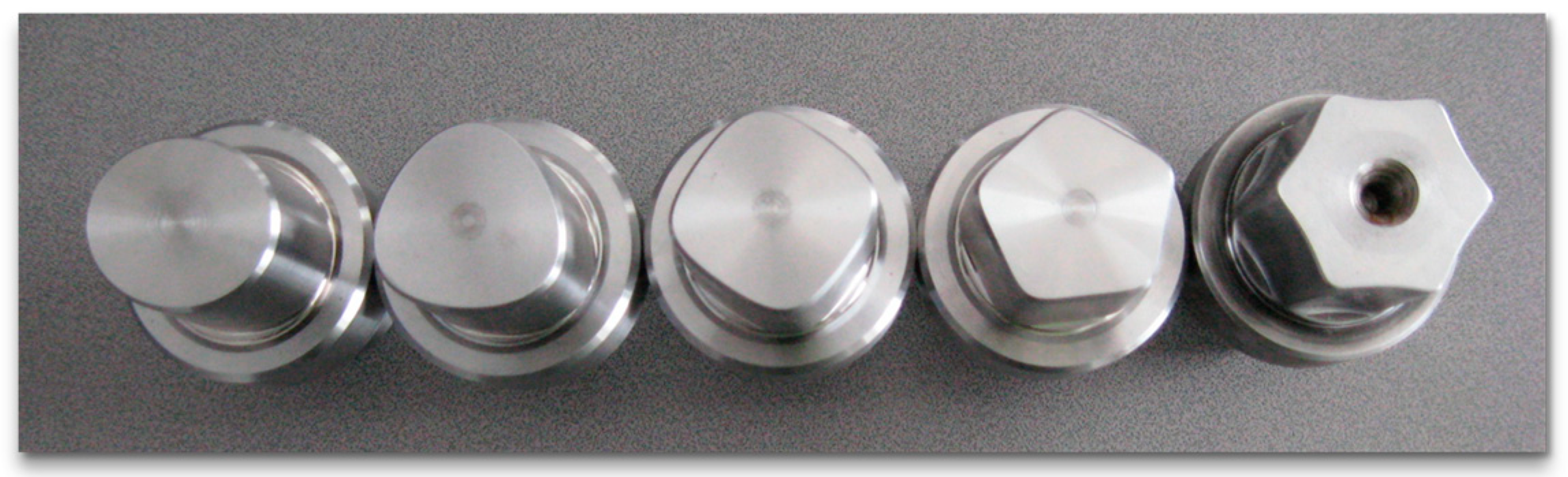
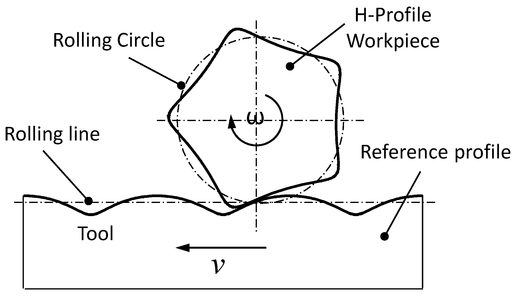
Additionally, a significant advantage of hypotrochoidal profiles (H-profiles) is their manufacturability through two-spindle turning [4,5] (Figure 2) and oscillating–turning [6] processes, as well as roller milling [7] (Figure 3). This allows time-efficient production.
Despite the excellent manufacturability described above and the great mechanical advantages of H-profiles, there is currently no reliable and cost-effective calculation method for the dimensioning of such profiles. The determination of the strength limit of H-profiles is still performed by means of extensive numerical investigations.
DIN 3689-1 refers to geometric specifications for H-profiles. Design guidelines are compiled in Part 2 of the standard. This paper represents an analytical solution for purely bending-loaded H-profile shafts in general and specifically for all standardised H-profiles for the first time. Furthermore, the author uses the analytical solution developed in another paper [8] for all standard profiles for torsional stresses and puts them together for practical and industrial applications.
The results can be used for a reliable and cost-effective calculation method of H-profile shafts with a simple pocket calculator for pure bending as well as torsional loads.
2. Geometry of H-Profiles
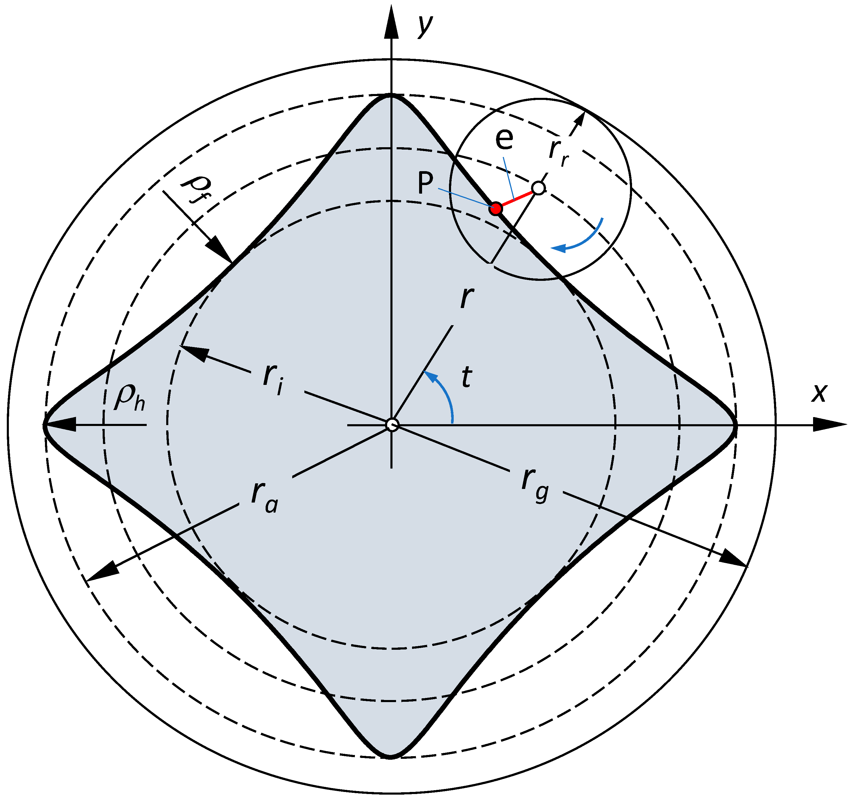
A hypotrochoid (H-profile) is created by rolling a circle with radius (called a rolling circle) on the inside of a guiding circle with radius with no slippage (see, for instance, [9]). The distance between the centre point of the rolling circle and the generating point P is defined as eccentricity (Figure 1). Depending on the diameter ratios of the two circles and the location of the generating point P in the rolling circle, different H-profiles may be formed.
The diameter ratio () defines the number of sides “n” and should be an integer () to obtain a closed curve without intersection. The coordinates of the generated point P describe the parameter equations for the hypotrochoid (H-profile) as follows:
The overlapping of the profile contour starts from the limit eccentricities of and, accordingly, the limit relative eccentricity of .
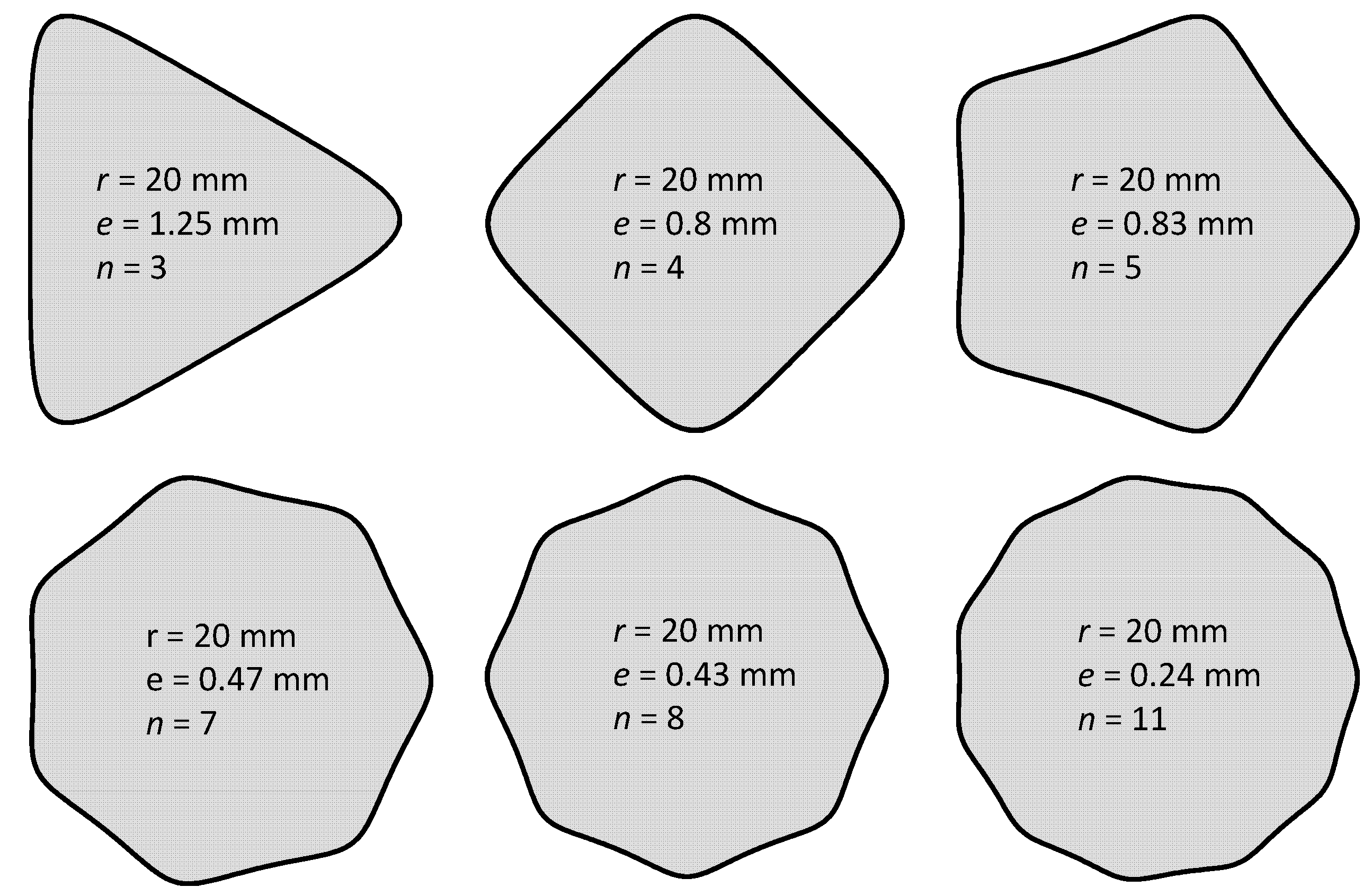
Figure 4 shows some examples of the H-profiles obtained for different numbers of sides (n) and eccentricities.
If a rolling circle rolls on the outside of a guiding circle, the profile generated is called an epicycloid (E-profile).
2.1. Geometric Properties
Area
Starting from the parameter representation (1) for the hypotrochoidal contours, the following complex mapping function is formulated as follows:
This function conformally maps the perimeter of a unit circle to the contour of a H-profile. However, when the area enclosed by the polygon was mapped, multiple poles were formed at the corners of the contour. A complete conformal mapping is not essential for the determination of bending stresses. However, for shear force bending, a complete mapping of profile cross-section is necessary (analogue to torsion problem [8]).
By substituting mapping (2) into the equation for the area [10,11]:
the following relationship can be derived for the area enclosed by an H-profile for any number of flanks n and eccentricity :
where is the first derivative of the mapping function, t defines the parameter angle, and is the area of the head circle (with ).
2.2. Radius of Curvature at Profile Corners and Flanks
From a manufacturing point of view, the radius of the curvature of the contour at profile corners (on the head circle) plays an important role. Using the equation presented in [11], the radius of curvature can be determined:
The second derivative of the mapping function in (5) is defined as .
The radius of curvature at profile corners (on the head circle in Figure 1) can be determined by substituting mapping function (2) into Equation (5) for t = 0 as follows:
The radius of curvature at profile corners is important in connection with the minimum tool diameter regarding the manufacturability of the profile.
The radius of curvature of the profile in the profile flank (Figure 1) can also be determined using Equation (5) for :
The radius of curvature in the flank area is a measure of the degree of the form closure of profile contours.
2.3. Bending Stresses
In many practical applications, a failure may occur in the profiled shaft outside of the connection due to the excessive stresses. For these cases, the following analytical approach based on [12] is used to solve the bending problem.
It is assumed that the cross-sections remain flat (without warping) after bending. The following relationships are valid for the stresses:
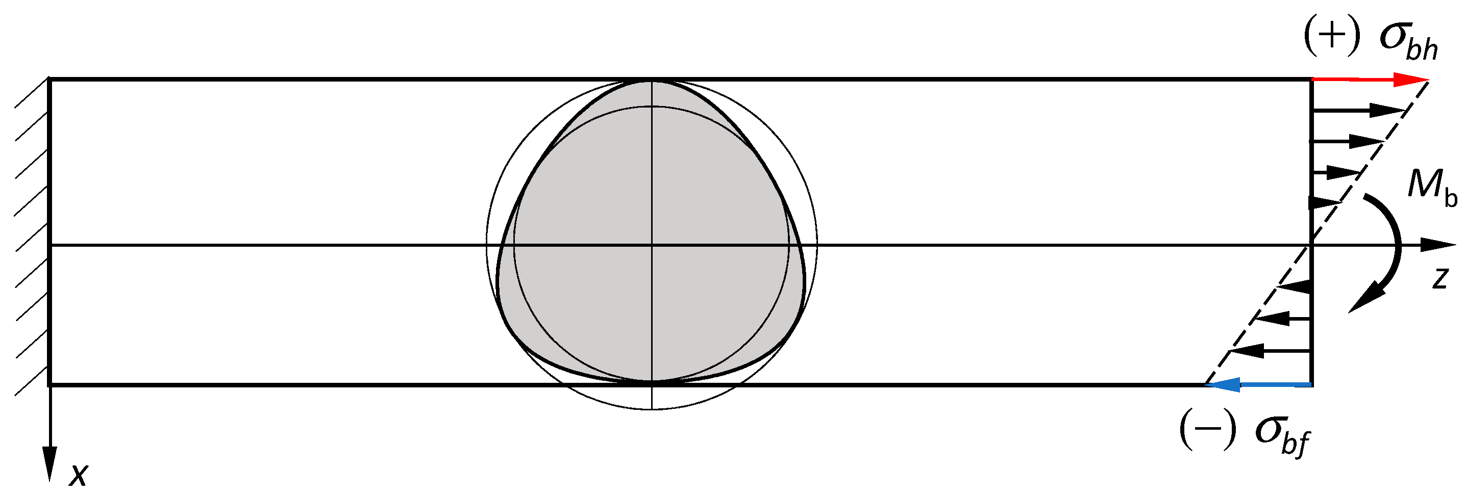
where denotes the moment of inertia for profile cross-section relative to the y-axis (Figure 5).
2.4. Bending Deformations
2.5. Moments of Inertia
The moments of inertia involve a double integral over the profile’s cross-section, but this can be reduced to a simple curvilinear integral over the profile contour using Green’s theorem, as follows:
The contour description according to Equation (2) is also advantageous here. For the contour of the profile’s cross-section, the following coordinates apply:
By substituting Equation (11) in (10), can be determined as such:
where . Function (12) facilitates the determination of moment of inertia with the assistance of Equation (2).
The moment of inertia is necessary for the calculation of the bending stress as well as for the determination of bending deformation (Equations (8) and (9)).
Inserting the mapping function from (2) into Equation (12) for , the following relationship is determined for the bending moment of inertia for an arbitrary number of flanks and eccentricity :
If one substitutes x(t) from (1) and from (13) into Equation (8), the distribution of the bending stress on the lateral surface of the profile can be determined as follows:
The maximum bending stress on the tension side occurs at (on the profile head, Figure 5), and therefore the following equation can be obtained:
The bending stress on the pressure side occurs at in the middle of a profile flank (on the profile foot, Figure 5) can also be determined as follows:
2.6. Example
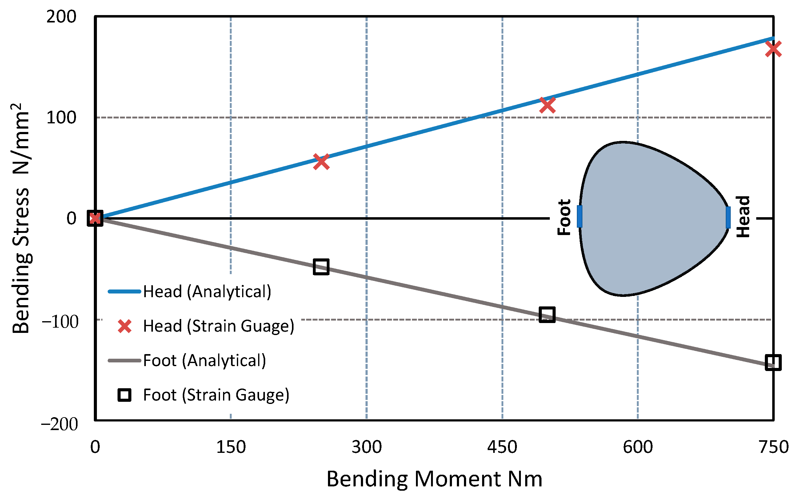
An H-profile from DIN 3689-1 [2] with three sides, a head circle diameter of 40 mm and eccentricity mm ( mm; related eccentricity ) was chosen as the object of investigation. The bending load was chosen as = 500 Nm.
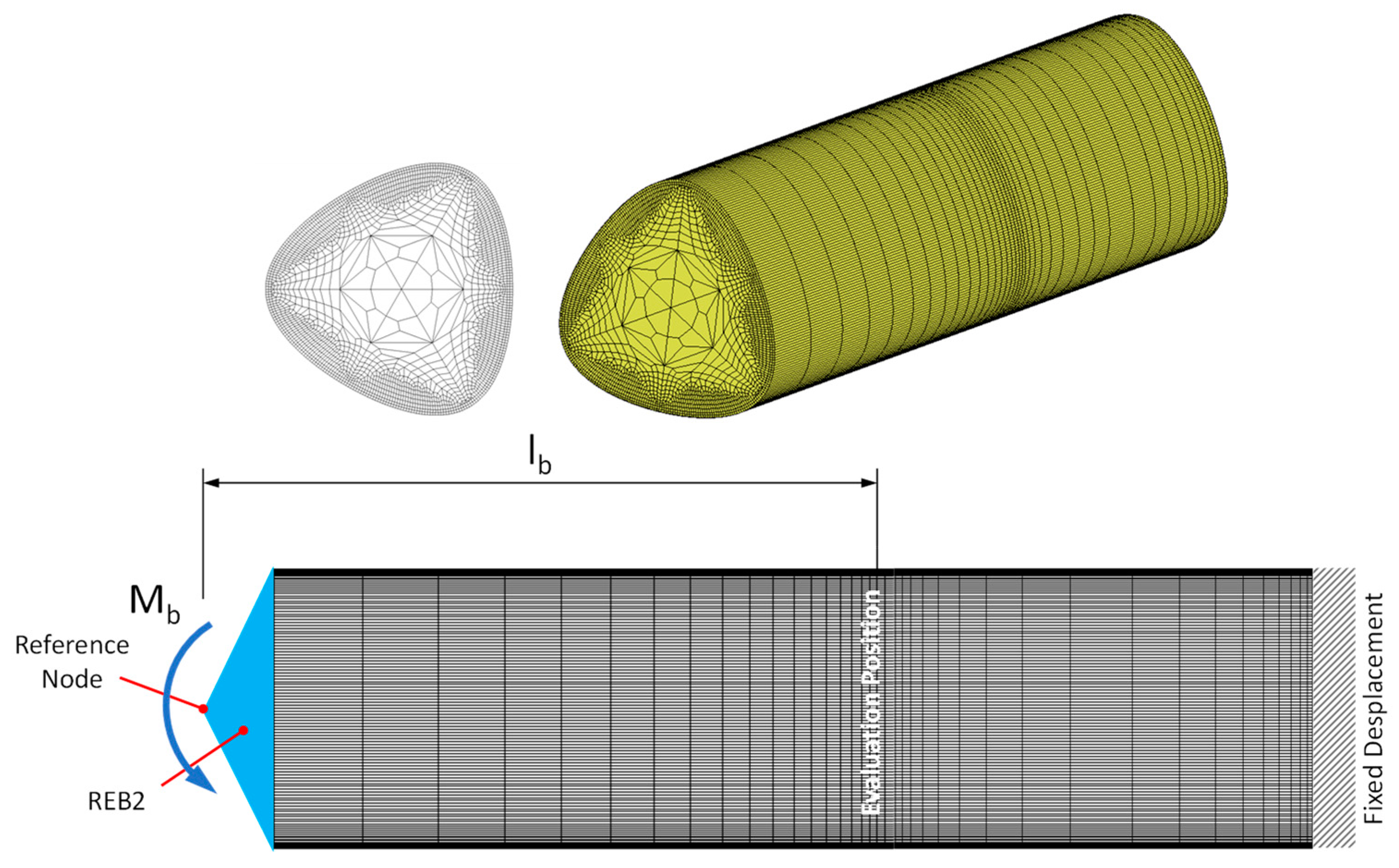
In order to compare the analytical results, numerical investigations were carried out using FE analyses, and the MSC-Marc programme system was used.
Figure 6 shows the mesh structure and the corresponding boundary conditions. The shaft is fixed on the right side. A bending moment is applied on the left side of the shaft via a reference node using REB2s. Bending stresses were evaluated at an adequate distance () from the loading point. The FE mesh in Figure 6 contains hexahedral elements with full integration, type 7 according to the Marc Element Library [14].
FE structures are generated by employing software written in Python language at the Chair of Machine Elements at West Saxon University of Zwickau, Germany. The FE meshes were then transferred to MSC-Marc program system and integrated into pre-processing.
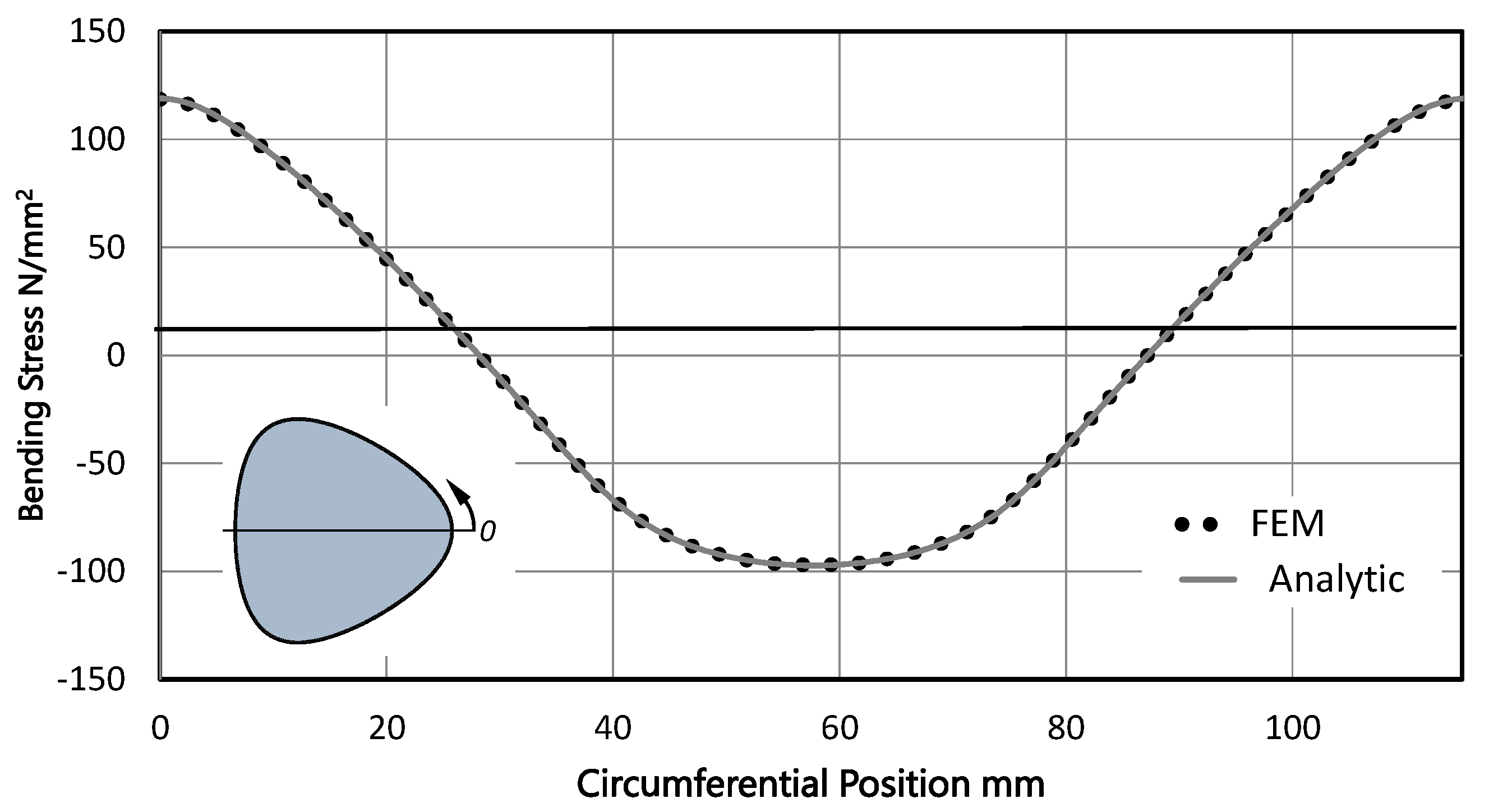
Figure 7 displays the distribution of bending stress on the circumference of the profile according to Equation (14) and its comparison with the numerical result. A good agreement between the results was observed.
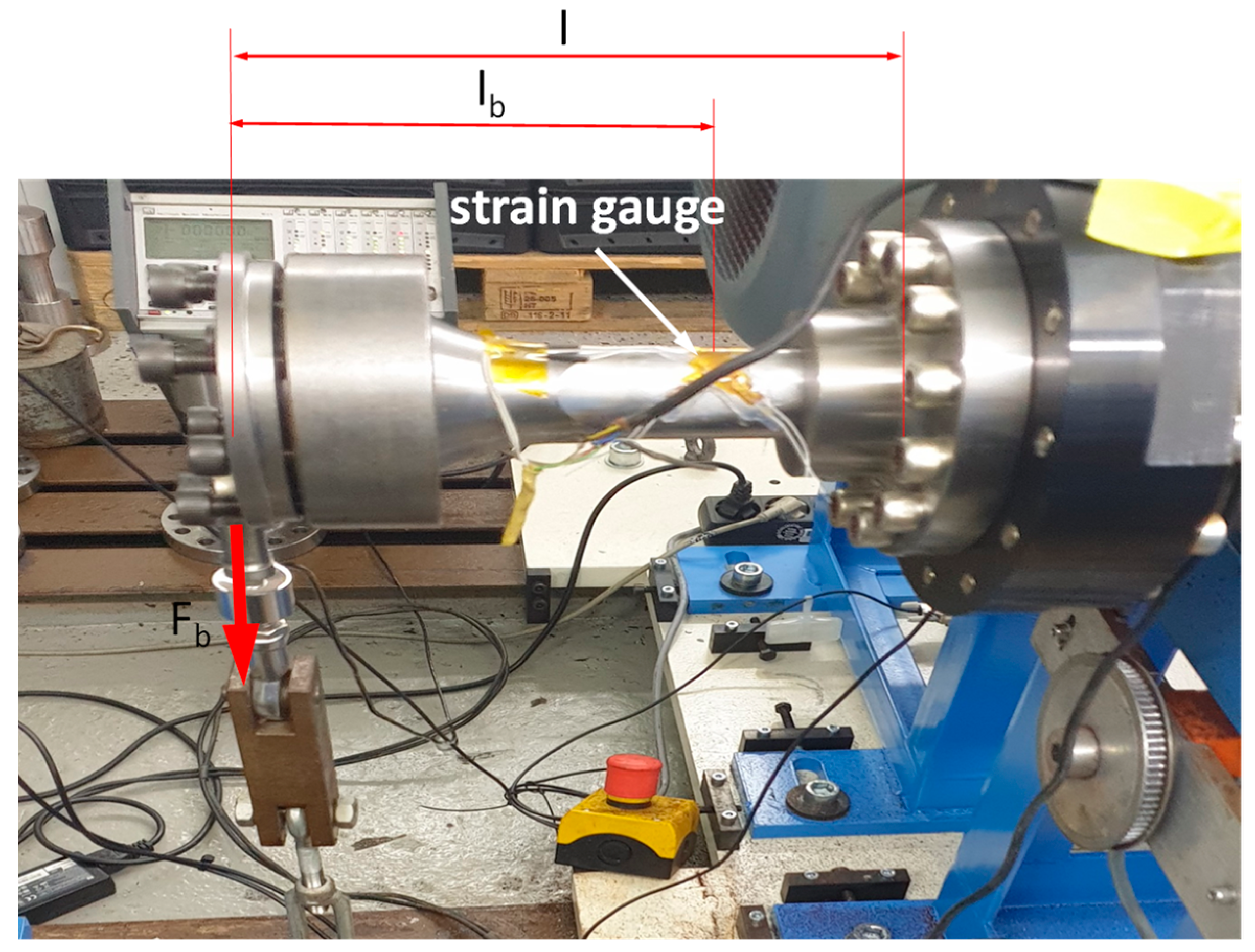
Additionally, bending stresses were experimentally determined for the profile head and foot areas. Figure 8 shows the test bench for bending load.
Experimental results for head and foot areas are compared with Equations (15) and (16) in Figure 9, where a good agreement of the results is evident.
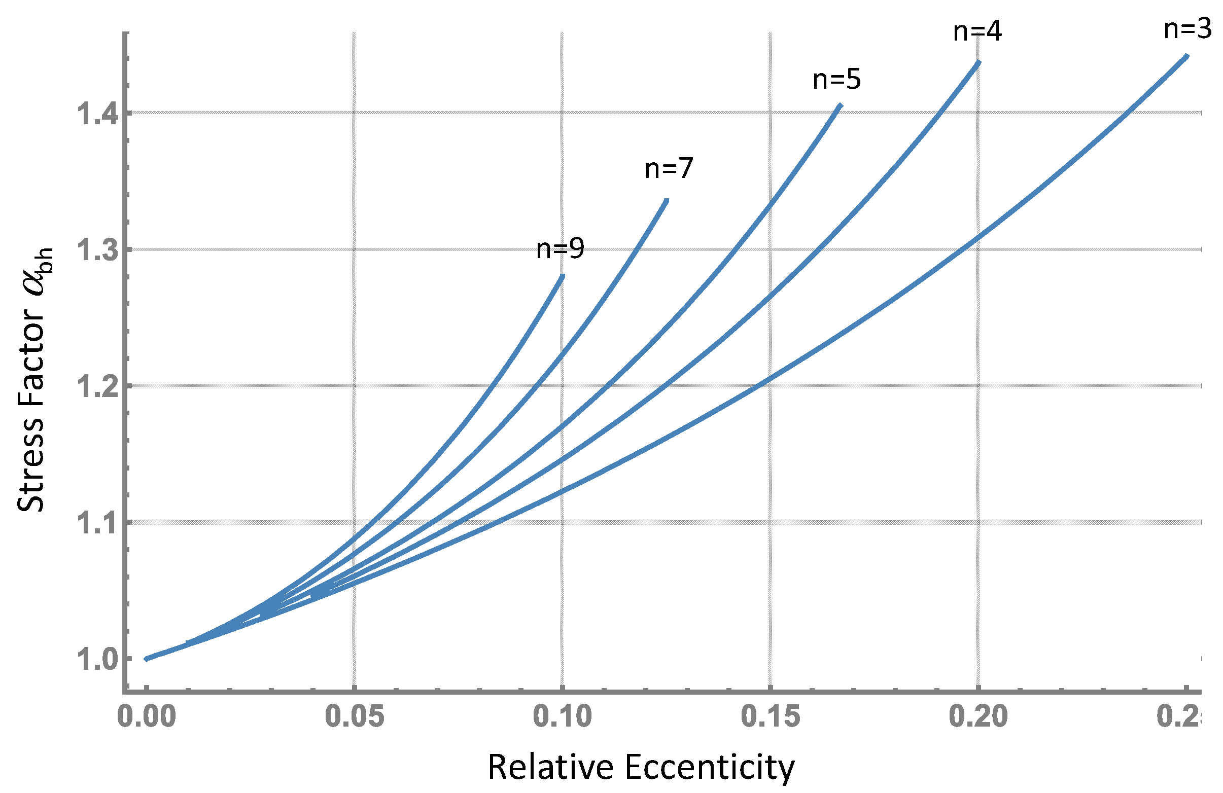
2.7. Stress Factor for Bending Loads
The stress factor is defined as the ratio of bending stress in a profile shaft to a corresponding reference stress for a round cross-section with radius (nomial radius of the profile):
For the head of the profile, the stress factor is determined as follows:
Figure 10 shows the curves for the stress factor as a function of the relative eccentricity for different numbers of sides . It can be recognised that the stress factor rises with an increase in eccentricity and or the number of sides.
For the profile base (foot), the following stress factor is analogously obtained:
2.8. Rotating Bending Stress
During power transmission, the gear shaft always shows rotational movement. Therefore, the rotating bending was also investigated.
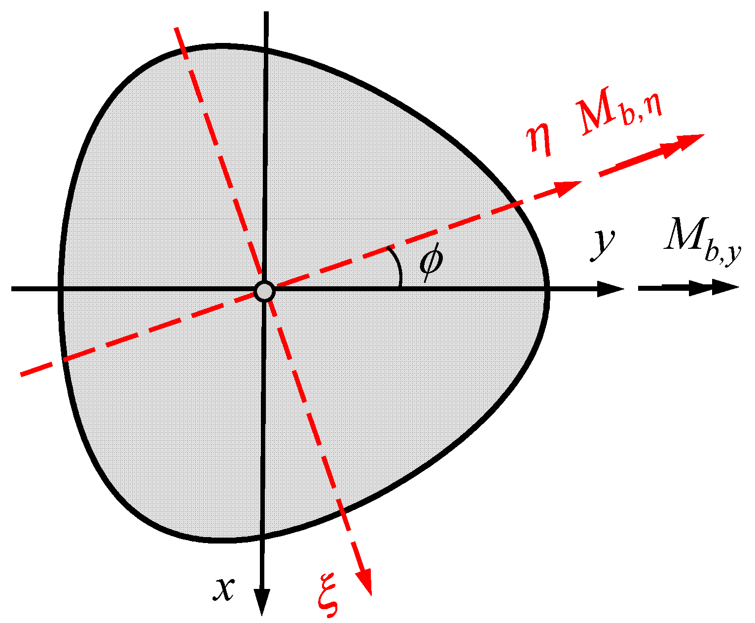
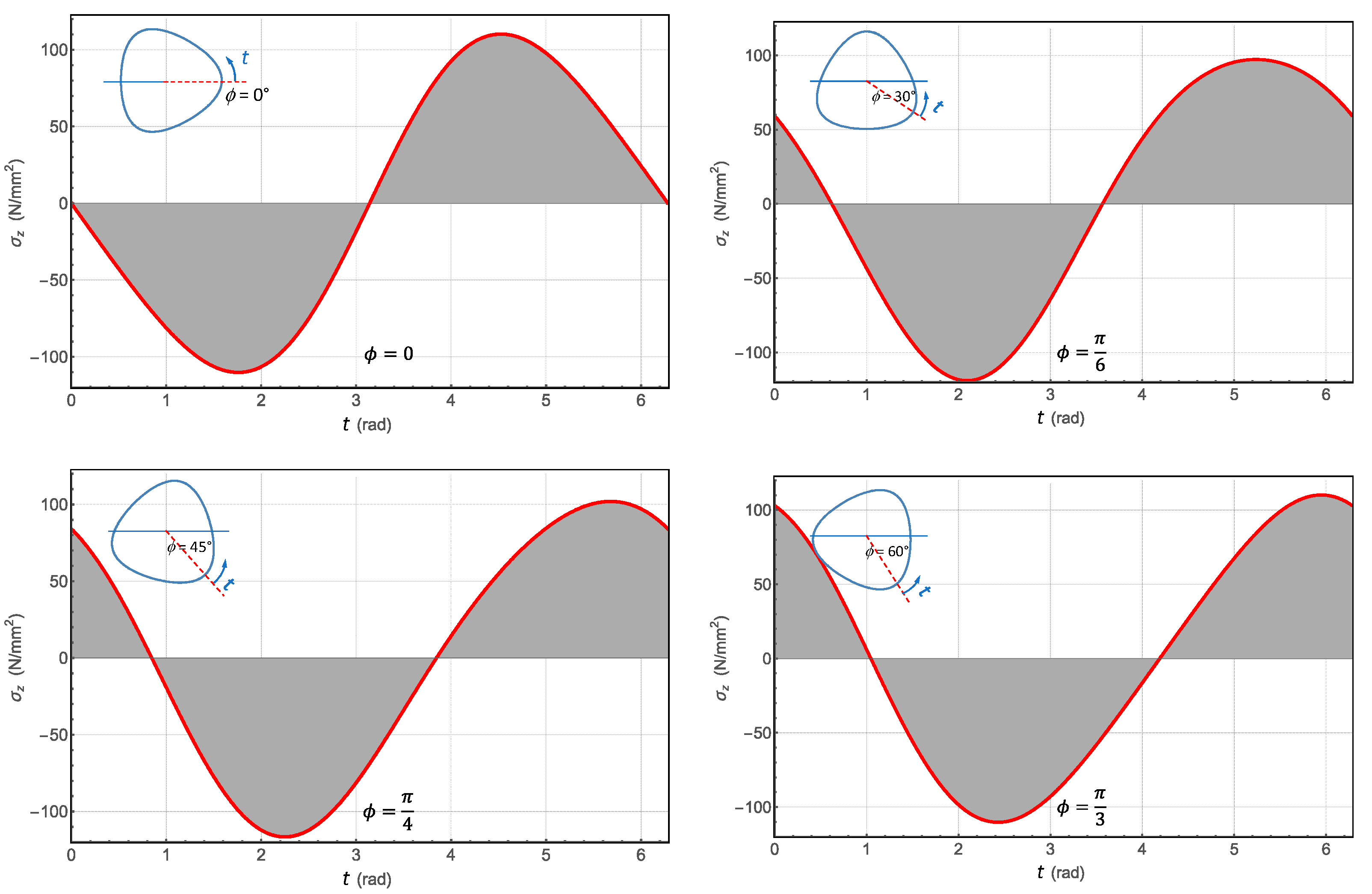
Figure 11 schematically represents the rotated position of an H-profile with three flanks according to the Cartesian coordinates.
The moment of inertia remains invariant due to the periodic symmetry of the cross-section of the H-profile presented based on Equation (2). Therefore, the following relationships are valid from Equation (12):
From Equation (20) and the use of Mohr’s circle, it can be proven that the moment of inertia is independent of the rotation angle (see also [10]):
In order to obtain the general solution of the bending stress according to Equation (8) for an arbitrary angle of rotation, the perpendicular distance is to be calculated in the rotated coordinate system:
where denotes the angle of rotation. If the values for x and y from (1) are inserted into the relationship (22), the following equation results for the perpendicular distance in the rotated coordinate system ():
The distribution of bending stress on the profile contour may be determined by using (23) in the relation of bending stress as follows:
Figure 12 shows the distributions of the bending stresses on the profile contour for different angles of rotation, which were determined using Equation (24). As expected, the maximum stress occurred at the profile head.
2.9. Deflection
The deflection of the profile shaft can also be determined with the help of the bending moment of inertia . As explained above, this is independent of the angular position of the cross-section (Equation (21)).
The deflection of the neutral axis is determined from Equation (9) for x = y = 0 as follows:
Substituting (13) in (25), the deflection can be determined as
2.10. Example
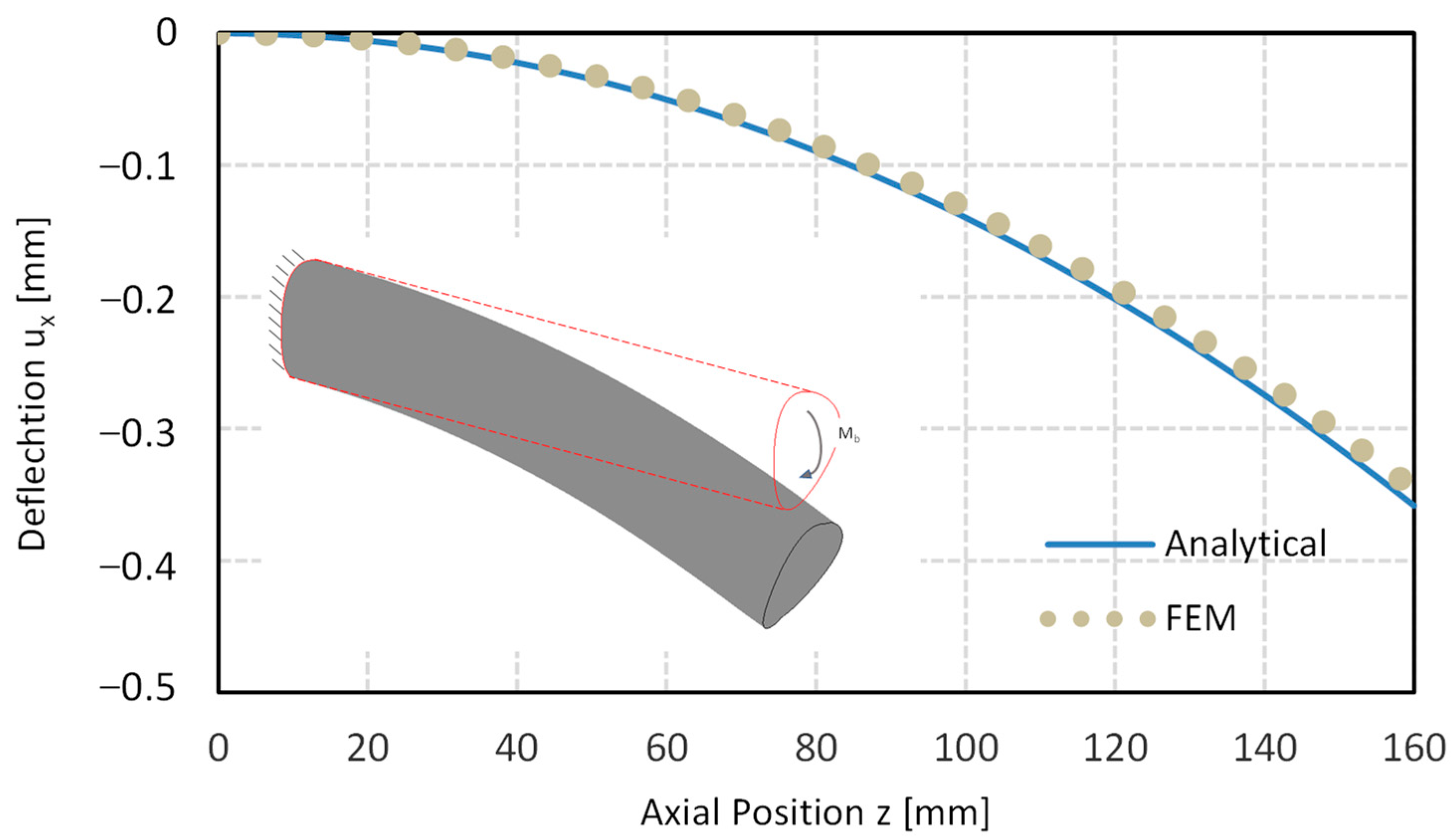
Figure 13 shows the deflection for an H-profile shaft with three flanks according to DIN3689-1 with = 40 mm (H3-40 × 32.73 with ε = 0.1) and a length of 160 mm made of steel (E = 210,000 ). The comparison with FE analysis shows very good agreement with Equation (26), as can also be seen in Figure 13. The bending load was chosen as = 500 Nm.
2.11. H-Profiles According to DIN3689-1
DIN3689-1 is a new standard that was published for the first time in November 2021. It describes the geometric properties of 18 specified H-profiles in two series. Series A is based on the head diameter, and series B involves the foot diameter as the nominal size of the profile. The respective corresponding profiles are geometrically similar. Each series contains 48 nominal sizes, which remain geometrically similar amongst themselves. Consequently, all standardised profiles are limited to 18 variants. This facilitates the processing of a generally valid design concept.
2.12. Stress Factor for Bending
The maximum bending stresses at the head and foot of the profile are important from a technical point of view for the design of a profile shaft subject to bending. Therefore, in this section, the two stress factors and for all the 18 standard profile series were determined using Equations (18) and (19).
2.13. Stress Factor for Torsion
The stress concentration factor for torsion is defined as the ratio of the maximum torsional stress (occurring in the middle of the profile flank) and the torsional stress in a round reference shaft with radius :
In [15], purely numerical investigations were carried out on the torsional stresses in H-profile shafts to calculate the stress factor.
The analytical solution for torsion may be performed using the approach of Muskhelishvili [12]. However, this requires a conformal mapping of the unit circle onto the polygon’s cross-section. For H-profiles, the mapping function derived from the parametric equation, Equation (1), cannot be directly used to solve the torsional stresses due to the multiple poles. The authors of [16] employed an elaborate computational process to determine the polynomials required for the description of the mappings of H-profiles. In [8,17,18,19], successive methods according to Kantorovich [20] were used to develop a suitable mapping function in the form of a series converging to the profile contour. The convergence quality and limit were examined and presented depending on the number of terms in the series developed in [8], calculating the torsional deformations for all standardised profiles. In the presented work, this method, accompanied by FEA, was used for all the 18 standardised profile geometries of DIN3689-1 to determine the maximum torsional stresses, which occur in the middle of the profile flank at the profile foot. A stress concentration factor for torsional loading was also determined analogously to that defined for the case of bending load.
For practical applications, the results for the bending and torsional stress factors are compiled in Table 1. Using the relative eccentricity, no dependence on the shaft diameter appears. Table 1 lists the results obtained for the bending and torsional stress factors for all standardised profile geometries according to DIN3689-1 (rounded to two decimal places).
The bending moment of the inertia of a circular cross-section with radius r is defined as a reference moment of inertia and labelled . The ratio between and is also listed in Table 1 for the standardised profiles. The H-profiles are normally slightly more flexible than round profiles.
3. Conclusions
In this paper, an analytical approach was presented to determine the bending stresses and deformations in the hypotrochoidal profile shafts. Valid calculation equations for the area, radii of curvature of the profile contour, and the bending moment of inertia were derived for such profiles. Furthermore, the solutions for bending stresses and deformations were presented. For practical applications, a stress factor was defined for the critical locations on the profile contour.
The analytical results demonstrated very good agreement with both numerical and experimentally determined results.
The stress factors of the bending stresses were determined for all profile geometries standardised according to DIN3689-1, and the values obtained were compiled in a table for practical applications. Based on previous works of the author, the stress factors for torsional stresses were also determined and added to the table. The data allow a reliable and cost-effective calculation of H-profile shafts with a pocket calculator for pure bending as well as torsional loads. This can be very advantageous for SMEs.
Funding
This research was funded by DFG (Deutsche Forschungsgemeinschaft) grant number [DFG ZI 1161/2].
Institutional Review Board Statement
Not applicable.
Informed Consent Statement
Not applicable.
Data Availability Statement
Not applicable.
Conflicts of Interest
The author declares no conflict of interest.
Abbreviations
| Formula Symbols: | ||
| mm2 | Area of profile cross-section | |
| mm | Profile eccentricity | |
| - | Euler’s number | |
| mm | Profile overlap eccentricity limit | |
| MPa | Young’s modulus | |
| - | Profile periodicity (number of sides) | |
| mm4 | Corresponding reference moments of inertia for a round cross-section with radius r | |
| mm4 | Torsional moment of inertia for reference shaft | |
| mm4 | Surface moments of inertia in the Cartesian coordinate system | |
| mm4 | Surface moment of inertia about y-axis for reference shaft | |
| mm4 | Surface moments of inertia in the rotated coordinate system | |
| mm | Length of profile shaft | |
| mm | Distance to strain gage in experimental test | |
| Nm | Bending moment | |
| mm | Nominal or mean radius | |
| - | Profile parameter angle | |
| mm | Displacement in x direction | |
| mm | Cartesian coordinates | |
| Greek Formula Symbols: | ||
| - | Bending stress factor for profile head | |
| - | Bending stress factor for profile foot | |
| - | Torsional stress factor for profile foot | |
| mm | deflection | |
| - | Relative eccentricity | |
| - | Rotation angle of the coordinate system | |
| - | Physical plane unit circle | |
| - | Polar angle | |
| MPa | Bending stress (z-component of stress vector) | |
| MPa | Torsional stress | |
| - | Completed mapping function | |
| - | Contour edge mapping function | |
| - | Complex variable in model plane | |
| - | Coordinates in rotated system | |
References
- DIN 6885-1:1968-08; Mitnehmerverbindungen ohne Anzug; Paßfedern, Nuten, Hohe Form. DIN-Deutsches Institut für Normung e.V.: Berlin, Germany, 1968.
- DIN 3689-1:2021-11; Welle-Nabe-Verbindung—Hypotrochoidische H-Profile—Teil 1: Geometrie und Maße. DIN-Deutsches Institut für Normung e.V.: Berlin, Germany, 2022.
- Selzer, M.; Forbrig, F.; Ziaei, M. Hypotrochoidische Welle-Nabe-Verbindungen. In Proceedings of the 9th Fachtagung Welle-Nabe-Verbindungen, Gestaltung Fertigung und Anwendung, Stuttgart, Germany, 26–27 November 2022; Band 2408. pp. 155–169. [Google Scholar]
- Gold, P.W. In acht Sekunden zum Polygon: Wirtschaftliches Unrunddrehverfahren zur Herstellung von Polygon-Welle-Nabe-Verbindungen. Antriebstechnik. Seiten 2006, 42–44. [Google Scholar]
- Iprotec GmbH, Polygonverbindungen. Bad Salzuflen, Germany. Available online: https://www.iprotec.de (accessed on 13 December 2022).
- Stenzel, H. Unrunddrehen und Fügen zweiteiliger Getriebezahnräder mit polygonaler Welle-Nabe-Verbindungen, VDI-4. Fachtagung Welle-Nabe-Verbindungen, Gestaltung Fertigung und Anwendung. Seiten 2010, 211–230. [Google Scholar]
- Ziaei, M. Westsächsische Hochschule Zwickau, Patentanmeldung: Application of Rolling Processes Using New Reference Profiles for the Production of Trochoidal Inner and Outer Contours. Patent-Nr. DE 10 2019 000 654 A1, 30 July 2020. [Google Scholar]
- Ziaei, M. Torsionsspannungen in Prismatischen, Unrunden Profilwellen mit Trochoidischen Konturen, Forschung im Ingenieurwesen; Ausgabe 4/2021; Springer: Berlin/Heidelberg, Germany, 2021; Available online: https://www.researchgate.net/publication/355421692_Torsionsspannungen_in_prismatischen_unrunden_Profilwellen_mit_trochoidischen_KonturenTorsional_stresses_and_deformations_in_prismatic_non-circular_profiled_shafts_with_trochoidal_contours (accessed on 14 December 2022).
- Bronstein, I.N.; Semendjajew, K.A. Taschenbuch der Mathematik, 7th Auflage; Verlag Hari Deutsch: Frankfurt am Main, Germany, 2008. [Google Scholar]
- Ziaei, M. Bending Stresses and Deformations in Prismatic Profiled Shafts with Noncircular Contours Based on Higher Hybrid Trochoids. Appl. Mech. 2022, 3, 1063–1079. [Google Scholar] [CrossRef]
- Zwikker, C. The Advanced Geometry of Plane Curves and Their Applications, Dover Books on Advanced Mathematics; Dover Publications: Mineola, NY, USA, 2005. [Google Scholar]
- Muskelishvili, N.I. Some Basic Problems of the Mathematical Theory of Elasticity; Springer: Dordrecht, The Netherlands, 1977. [Google Scholar]
- Sokolnikoff, I.S. Mathematical Theory of Elasticity; Robert E. Krieger Publishing Company: Malaba, FL, USA, 1983. [Google Scholar]
- Marc 2020 Manual; Volume B (Element Library); MSC Software Corporation: Newport Beach, CA, USA, 2020.
- Schreiter, R. Numerische Untersuchungen zu Form- und Kerbwirkungszahlen von Hypotrochoidischen Polygonprofilen unter Torsionsbelastung; Dissertation TU Chemnitz: Chemnitz, Germany, 2022. [Google Scholar]
- Ivanshin, P.N.; Shirokova, E.A. Approximate Conformal Mappings and Elasticity Theory. J. Complex Anal. Hindawi Publ. Corp. 2016, 2016, 4367205. [Google Scholar] [CrossRef] [Green Version]
- Ziaei, M. Analytische Untersuchung Unrunder Profilfamilien und Numerische Optimierung Genormter Polygonprofile für Welle-Nabe-Verbindungen, Habilitationsschrift; Technische Universität Chemnitz: Chemnitz, Germany, 2002. [Google Scholar]
- Research Report: Entwicklung eines analytischen Berechnungskonzeptes für formschlüssige Welle-Nabe-Verbindungen mit hypotrochoidischen Verbindungen, Abschlussbericht zum DFG-Vorhaben DFG ZI 1161/2 (Westsächsische Hochschule Zwickau) und LE 969/21(TU Chemnitz); Westsächsische Hochschule Zwickau: Zwickau, Germany, 2020.
- Lee, K. Mechanical Analysis of Fibers with a Hypotrochoidal Cross Section by Means of Conformal Mapping Function. Fibers Polym. 2010, 11, 638–641. [Google Scholar] [CrossRef]
- Kantorovich, L.V.; Krylov, V.I. Approximate Methods of Higher Analysis; Dover Publications: Mineola, NY, USA, 2018. [Google Scholar]
Figure 1.
Description of exemplary hypotrochoid (H-profile) with four concave sides. A detailed explanation of the parameters is given below in Section 2.
Figure 1.
Description of exemplary hypotrochoid (H-profile) with four concave sides. A detailed explanation of the parameters is given below in Section 2.

Figure 2.
Some H-profiles manufactured by two-spindle process, Iprotec GmbH, © Guido Kochsiek, www.iprotec.de, Zwiesel, Germany [5].
Figure 2.
Some H-profiles manufactured by two-spindle process, Iprotec GmbH, © Guido Kochsiek, www.iprotec.de, Zwiesel, Germany [5].

Figure 3.
Roller milling manufacturing for H-profile [7].
Figure 3.
Roller milling manufacturing for H-profile [7].

Figure 4.
Examples of H-profiles with different numbers of sides (n) and eccentricities.

Figure 5.
The bending coordinate system for a loaded profile shaft.

Figure 6.
FE mesh and boundary conditions for the H-profile with n = 3 according to DIN 3689-1.

Figure 7.
Circumferential distribution of the bending stress on the lateral surface of a standardised H3 profile.
Figure 7.
Circumferential distribution of the bending stress on the lateral surface of a standardised H3 profile.

Figure 8.
Bending loads test bench (Machine Elements Laboratory at West Saxon University of Zwickau).
Figure 8.
Bending loads test bench (Machine Elements Laboratory at West Saxon University of Zwickau).

Figure 9.
Comparison of the experimental results with the analytical solutions.

Figure 10.
Stress factors for the bending stress at the profile head (Equation (18)) with varying relative eccentricity and number of sides.
Figure 10.
Stress factors for the bending stress at the profile head (Equation (18)) with varying relative eccentricity and number of sides.

Figure 11.
Rotated coordinate system for determining the bending moment of inertia.

Figure 12.
Distributions of the bending stresses on the profile contour for different angles of rotation , with mm, , mm, and = 500 Nm.
Figure 12.
Distributions of the bending stresses on the profile contour for different angles of rotation , with mm, , mm, and = 500 Nm.

Figure 13.
Deflection in a DIN3689-H3-40 × 32.73 profile shaft.


Table 1.
Stress factors for bending and torsional loads for the H-profiles standardised according to DIN3689-1.
Table 1.
Stress factors for bending and torsional loads for the H-profiles standardised according to DIN3689-1.
| 3 | 0.100 | 1.12 | 0.92 | 0.98 | 1.23 |
| 4 | 0.056 | 1.07 | 0.96 | 0.99 | 1.17 |
| 4 | 0.111 | 1.17 | 0.94 | 0.95 | 1.37 |
| 5 | 0.031 | 1.04 | 0.97 | 0.99 | 1.12 |
| 5 | 0.062 | 1.09 | 0.96 | 0.98 | 1.24 |
| 5 | 0.094 | 1.16 | 0.96 | 0.95 | 1.38 |
| 6 | 0.020 | 1.02 | 0.98 | 1.00 | 1.10 |
| 6 | 0.040 | 1.05 | 0.97 | 0.99 | 1.18 |
| 6 | 0.062 | 1.10 | 0.97 | 0.97 | 1.37 |
| 7 | 0.028 | 1.04 | 0.98 | 0.99 | 1.15 |
| 7 | 0.056 | 1.09 | 0.97 | 0.97 | 1.29 |
| 7 | 0.083 | 1.16 | 0.99 | 0.93 | 1.43 |
| 9 | 0.023 | 1.03 | 0.98 | 0.99 | 1.17 |
| 9 | 0.047 | 1.08 | 0.98 | 0.97 | 1.31 |
| 9 | 0.062 | 1.12 | 0.99 | 0.95 | 1.39 |
| 12 | 0.017 | 1.02 | 0.99 | 0.99 | 1.16 |
| 12 | 0.033 | 1.06 | 0.99 | 0.98 | 1.28 |
| 12 | 0.050 | 1.10 | 1.00 | 0.95 | 1.38 |
Disclaimer/Publisher’s Note: The statements, opinions and data contained in all publications are solely those of the individual author(s) and contributor(s) and not of MDPI and/or the editor(s). MDPI and/or the editor(s) disclaim responsibility for any injury to people or property resulting from any ideas, methods, instructions or products referred to in the content. |
© 2023 by the author. Licensee MDPI, Basel, Switzerland. This article is an open access article distributed under the terms and conditions of the Creative Commons Attribution (CC BY) license (https://creativecommons.org/licenses/by/4.0/).
Share and Cite
MDPI and ACS Style
Ziaei, M. Bending and Torsional Stress Factors in Hypotrochoidal H-Profiled Shafts Standardised According to DIN 3689-1. Eng 2023, 4, 829-842. https://doi.org/10.3390/eng4010050
AMA Style
Ziaei M. Bending and Torsional Stress Factors in Hypotrochoidal H-Profiled Shafts Standardised According to DIN 3689-1. Eng. 2023; 4(1):829-842. https://doi.org/10.3390/eng4010050
Chicago/Turabian StyleZiaei, Masoud. 2023. "Bending and Torsional Stress Factors in Hypotrochoidal H-Profiled Shafts Standardised According to DIN 3689-1" Eng 4, no. 1: 829-842. https://doi.org/10.3390/eng4010050