Article

Highly Dispersive Optical Solitons in Birefringent Fibers of Complex Ginzburg–Landau Equation of Sixth Order with Kerr Law Nonlinear Refractive Index

by
Elsayed M. E. Zayed
1,
Khaled A. Gepreel
1,2,
Mahmoud El-Horbaty
1 and
Mohamed E. M. Alngar
3,*
1
Mathematics Department, Faculty of Sciences, Zagazig University, Zagazig 44519, Egypt
2
Mathematics Department, Faculty of Sciences, Taif University, P.O. Box 11099, Taif 21944, Saudi Arabia
3
Basic Science Department, Faculty of Computers and Artificial Intelligence, Modern University for Technology & Information, Cairo 11585, Egypt
*
Author to whom correspondence should be addressed.
Eng 2023, 4(1), 665-677; https://doi.org/10.3390/eng4010040
Submission received: 6 January 2023 / Revised: 8 February 2023 / Accepted: 15 February 2023 / Published: 17 February 2023
(This article belongs to the Section Electrical and Electronic Engineering)

Abstract

:
In this paper, we derived optical soliton solutions with a highly dispersive nonlinear complex Ginzburg–Landau (CGL) equation in birefringent fibers that have Kerr law nonlinearity. We applied two mathematical methods, namely the addendum Kudryashov’s method and the unified Riccati equation expansion method. Straddled solitary solutions, bright soliton, dark soliton and singular soliton solutions were obtained.This model represents the propagation of a dispersive optical soliton through a birefringent fiber. This happens when pulses propagating through an optical fiber split into two pulses.

1. Introduction

It is well recognized that nonlinear partial differential equations play a vital role in physics and engineering challenges, where they are commonly utilized to represent many complicated phenomena, such as optical fibers, plasma physics, fluid mechanics, biology, chemical kinetics, and so on. In fact, explicit analytical solutions of these equations can be found using several mathematical methods. There are numerous systems, including the Lakshmanan–Porsezian–Daniel (LPD) model, the Radhakrishnan–Kundu–Lakshmanan (RKL) equation, the Gabitov–Turisyn (GT) equation, the Schrodinger–Hirota (SH) equation, the complex Ginzburg–Landau (CGL) equation, the Fokas–Lenell’s (FL) equation [1,2,3,4,5,6,7,8,9,10,11,12,13,14,15,16,17,18,19,20,21,22,23,24,25,26,27,28,29,30,31,32,33,34,35,36] and so on. These are well-known examples of fibers that maintain polarization. The Manakov equation and the Thirring model are two examples of common models for studying split pulses in birefringent fibers. The underlying dynamics of soliton wave propagation for each of these models is the existence of a careful balance between self-phase modulation (SPM) and chromatic dispersion (CD). When the CD is low, an unreasonable result can happen, pending the transmission of optical fiber pulses. To get around this crisis, a variety of technology backup plans have been put into action. One suggestion is to use Bragg gratings with dispersive reflectivity to make up for the low CD count. Pure-quartic solitons were introduced as a different strategy throughout.
In this case, the CD is mutated by 4th-order dispersion (4OD). The disadvantage of such a model is that, for pure-quartic NLSE, one can only recover stationary optical solitons analytically and it can only be analyzed numerically. As a result, pure-quartic solitons were never widely adopted as a substitute paradigm to deal with the dilemma. Then, the fundamental idea of cubic-quartic (CQ) solitons emerged, replacing CD with fourth-order dispersion (4OD) and third-order dispersion (3OD) jointly [21,22]. The advent of the torrent of analytical results in the flow is proof that these topics have recently attracted considerable interest. In this context, sixth-order dispersion (6OD)), fifth-order dispersion (5OD), fourth-order dispersion (4OD), third-order dispersion (3OD)) and the inter- modal dispersion (IMD) terms are considered, in addition to the pre-existing CD, which, together, make up the HD solitons that provide the necessary delicate balance between self-phase modulation (SPM) and CD for the solitons to sustain the inter-continental distance propagation.

Governing Model

The highly dispersive perturbed complex Ginzburg–Landau equation with the Kerr law refractive index in polarization-preserving fiber is well known [28] and reads as:
i q t + i a 1 q x + a 2 q x x + i a 3 q x x x + a 4 q x x x x + i a 5 q x x x x x + a 6 q x x x x x x + c q 2 q = α q x 2 q * + β 4 q 2 q * 2 q 2 q 2 x x q 2 x 2 + γ q + i [ λ ( q 2 m q ) x + μ ( q 2 m ) x q + υ q 2 m q x ]
where q ( x , t ) is the wave profile of the solution, which is a complex-valued function, q * is the complex conjugate and i 2 = 1 . Here, a j ( j = 1 6 ) , c , α , β , γ , λ , μ , υ and m are real constants. The first term in Equation (1) is the linear temporal evolution. The constant a 1 is the inter-model dispersion (IMD), the constant a 2 is the chromatic dispersion (CD), the constant a 3 is the 3OD, the constant a 4 is the 4OD, the constant a 5 is the 5OD and the constant a 6 is the 6OD. The constant c is the coefficient of the Kerr law of nonlinearity. The constants α , β , μ , υ are the coefficients of nonlinear dispersions. Finally, γ and λ are the coefficients of self-detuning and self-steepening terms, respectively. The objective of this article is to study the following two couples of CGLE in birefringent fibers, which are written for the first time as follows:
i u t + i a 1 u x + a 2 u x x + i a 3 u x x x + a 4 u x x x x + i a 5 u x x x x x + a 6 u x x x x x x + ( c 1 u 2 + d 1 v 2 ) u = 1 u * [ α 1 u x 2 + β 1 v x 2 + σ 1 u 2 x x + δ 1 v 2 x x ] 1 ( μ 1 u 2 + ζ 1 v 2 ) u * θ 1 u 2 x 2 + γ 1 u 2 x v 2 x + ρ 1 v 2 x 2 + ψ 1 u + i [ λ 1 ( u 2 m u ) x + E 1 ( u 2 m ) x u + υ 1 u 2 m u x ] ,
and
i v t + i b 1 v x + b 2 v x x + i b 3 v x x x + b 4 v x x x x + i b 5 v x x x x x + b 6 v x x x x x x + ( c 2 v 2 + d 2 u 2 ) v = 1 v * [ α 2 v x 2 + β 2 u x 2 + σ 2 v 2 x x + δ 2 u 2 x x ] 1 ( μ 2 v 2 + ζ 2 u 2 ) v * θ 2 v 2 x 2 + γ 2 v 2 x u 2 x + ρ 2 u 2 x 2 + ψ 2 v + i [ λ 2 ( v 2 m v ) x + E 2 ( v 2 m ) x v + υ 2 v 2 m v x ] ,
where u ( x , t ) and v ( x , t ) are complex-valued functions that reflect the wave profiles and a j , b j ( j = 1 6 ) , c k , d k , α k , β k , σ k , δ k , θ k , γ k , ρ k , μ k , ζ k , ψ k , λ k , E k , υ k ( k = 1 , 2 ) are real-valued constants. Its c k , d k ( k = 1 , 2 ) are the self-phase modulation (SPM) coefficients and the cross-phase modulation (XPM) coefficients, respectively. The terms owing to α k , β k , δ k , σ k , μ k , ζ k , θ k , γ k , ρ k , ψ k ( k = 1 , 2 ) are the perturbation effect; in particular, ψ k is obtained by the detuning effect, λ k are the self-steepening (SS) coefficient terms and the nonlinear terms coefficients used to discuss optical solutions are E k and υ k . The objective of this article is to solve Equations (2) and (3) utilizing the addendum Kudryashov method and the unified Riccati equation expansion approach.
The current paper is an analysis of HD-CGLE but in birefringent fibers. It is worth mentioning that the model is addressed in a single channel but in birefringent fibers with the Kerr law nonlinear refractive index. These are the familiar erbium-doped fibers with the presence of a 3OD effect, in addition to CD and STD. This is a differential group delay (DGD) effect after the occurrence of pulse splitting. The accumulation of such a DGD leads to the effect of birefringence. Thus, HD-CGLE in birefringent fibers is the focus of attention in this work. The above system (2) and (3) is more general than that obtained in the articles [10,11,12,13,14,15,16,17,18,21,22,23,27,28], and our results are different and new.
The structure of this article is ordered as follows: the introduction is in Section 1. Section 2 discusses the mathematical foundations. In order to determine the optical soliton solutions for the system (1) and (2), we use the addendum to Kudryashov’s in Section 3 and the unified Riccati equation expansion approach in Section 4. Numerical simulations are presented in Section 5. Conclusions are demonstrated in Section 6.

2. Mathematical Preliminaries

We will consider the transformations of traveling waves as
u ( x , t ) = ϕ 1 ( ξ ) e i ( κ x + w t + θ 0 ) ,
v ( x , t ) = ϕ 2 ( ξ ) e i ( κ x + w t + θ 0 ) ,
where ϕ j ( ξ ) ( j = 1 , 2 ) are real-valued functions representing the traveling waves’ amplitudes, ξ = x V t . Here, V is the velocity of the solitons, κ its frequency, w is the wave number and θ 0 is the phase constant. Substituting (4) and (5) into Equations (2) and (3) and separating the real and imaginary parts, we obtain the real parts as follows:
k ( λ 1 + υ 1 ) ϕ 1 2 m + 2 ( ζ 1 ϕ 2 2 + μ 1 ϕ 1 2 ) + d 1 ζ 1 ϕ 1 2 ϕ 2 4 β 1 k 2 ϕ 1 2 ( ζ 1 ϕ 2 2 + μ 1 ϕ 1 2 ) + ( c 1 ζ 1 + d 1 μ 1 ) ϕ 1 4 ϕ 2 2 2 δ 1 ( ζ 1 ϕ 2 2 + μ 1 ϕ 1 2 ) ϕ 2 ϕ 2 + a 6 ( ζ 1 ϕ 2 2 + μ 1 ϕ 1 2 ) ϕ 1 ϕ 1 ( 6 ) + ( 15 a 6 k 2 + 5 a 5 k + a 4 ) ( ζ 1 ϕ 2 2 + μ 1 ϕ 1 2 ) ϕ 1 ϕ 1 ( 4 ) + ( 15 a 6 k 4 10 a 5 k 3 6 a 4 k 2 + 3 a 3 k + a 2 2 σ 1 ) ( ζ 1 ϕ 2 2 + μ 1 ϕ 1 2 ) ϕ 1 ϕ 1 + ( a 6 k 6 + a 5 k 5 + a 4 k 4 a 3 k 3 a 2 k 2 α 1 k 2 + a 1 k ψ 1 w ) ϕ 1 2 ( ζ 1 ϕ 2 2 + μ 1 ϕ 1 2 ) [ ( α 1 ζ 1 + 2 σ 1 ζ 1 ) ϕ 2 2 + ( α 1 μ 1 + 2 σ 1 μ 1 4 θ 1 ) ϕ 1 2 ] ( ϕ 1 ) 2 + 4 γ 1 ϕ 1 ϕ 2 ϕ 1 ϕ 2 [ ( β 1 ζ 1 + 2 δ 1 ζ 1 4 ρ 1 ) ϕ 2 2 + ( β 1 μ 1 + 2 δ 1 μ 1 ) ϕ 1 2 ] ( ϕ 2 ) 2 + c 1 μ 1 ϕ 1 6 = 0 ,
k ( λ 2 + υ 2 ) ϕ 2 2 m + 2 ( ζ 2 ϕ 1 2 + μ 2 ϕ 2 2 ) + d 2 ζ 2 ϕ 2 2 ϕ 1 4 β 2 k 2 ϕ 2 2 ( ζ 2 ϕ 1 2 + μ 2 ϕ 2 2 ) + ( c 2 ζ 2 + d 2 μ 2 ) ϕ 2 4 ϕ 1 2 2 δ 1 ( ζ 2 ϕ 1 2 + μ 2 ϕ 2 2 ) ϕ 1 ϕ 1 + b 6 ( ζ 2 ϕ 1 2 + μ 2 ϕ 2 2 ) ϕ 2 ϕ 2 ( 6 ) + ( 15 b 6 k 2 + 5 b 5 k + b 4 ) ( ζ 2 ϕ 1 2 + μ 2 ϕ 2 2 ) ϕ 2 ϕ 2 ( 4 ) + ( 15 b 6 k 4 10 b 5 k 3 6 b 4 k 2 + 3 b 3 k + b 2 2 σ 2 ) ( ζ 2 ϕ 1 2 + μ 2 ϕ 2 2 ) ϕ 2 ϕ 2 + ( b 6 k 6 + b 5 k 5 + b 4 k 4 b 3 k 3 b 2 k 2 α 2 k 2 + b 1 k ψ 2 w ) ϕ 2 2 ( ζ 2 ϕ 1 2 + μ 2 ϕ 2 2 ) [ ( α 2 ζ 2 + 2 σ 2 ζ 2 ) ϕ 1 2 + ( α 2 μ 2 + 2 σ 2 μ 2 4 θ 2 ) ϕ 2 2 ] ( ϕ 2 ) 2 + 4 γ 2 ϕ 2 ϕ 1 ϕ 2 ϕ 1 [ ( β 2 ζ 2 + 2 δ 2 ζ 2 4 ρ 2 ) ϕ 1 2 + ( β 2 μ 2 + 2 δ 2 μ 2 ) ϕ 2 2 ] ( ϕ 1 ) 2 + c 2 μ 2 ϕ 2 6 = 0 ,
and the imaginary parts:
ζ 1 [ 2 E 1 m + 2 λ 1 m + λ 1 + υ 1 ] ϕ 1 2 m + 1 ϕ 2 2 ϕ 1 μ 1 ( 2 E 1 m + 2 m λ 1 + λ 1 + υ 1 ) ϕ 1 2 m + 3 ϕ 1 ζ 1 ( 6 a 6 k 5 + 5 a 5 k 4 + 4 a 4 k 3 3 a 3 k 2 2 a 2 k V + a 1 ) ϕ 1 ϕ 2 2 ϕ 1 + ζ 1 ( 6 a 6 k + a 5 ) ϕ 1 ϕ 2 2 ϕ 1 ( 5 ) + ζ 1 ( 20 a 6 k 3 10 a 5 k 2 4 a 4 k + a 3 ) ϕ 1 ϕ 2 2 ϕ 1 + μ 1 ( 6 a 6 k 5 + 5 a 5 k 4 + 4 a 4 k 3 3 a 3 k 2 2 a 2 k V + a 1 ) ϕ 1 3 ϕ 1 + μ 1 ( 20 a 6 k 3 10 a 5 k 2 4 a 4 k + a 3 ) ϕ 1 3 ϕ 1 + μ 1 ( 6 a 6 k + a 5 ) ϕ 1 3 ϕ 1 ( 5 ) = 0 , .
ζ 2 [ 2 E 2 m + 2 λ 2 m + λ 2 + υ 2 ] ϕ 2 2 m + 1 ϕ 1 2 ϕ 2 μ 2 ( 2 E 2 m + 2 m λ 2 + λ 2 + υ 2 ) ϕ 2 2 m + 3 ϕ 2 + ζ 2 ( 6 b 6 k 5 + 5 b 5 k 4 + 4 b 4 k 3 3 b 3 k 2 2 b 2 k V + b 1 ) ϕ 2 ϕ 1 2 ϕ 2 + ζ 2 ( 6 b 6 k + b 5 ) ϕ 2 ϕ 1 2 ϕ 2 ( 5 ) + ζ 2 ( 20 b 6 k 3 10 b 5 k 2 4 b 4 k + b 3 ) ϕ 2 ϕ 1 2 ϕ 2 + μ 2 ( 6 b 6 k 5 + 5 b 5 k 4 + 4 b 4 k 3 3 b 3 k 2 2 b 2 k V + b 1 ) ϕ 2 3 ϕ 2 + μ 2 ( 20 b 6 k 3 10 b 5 k 2 4 b 4 k + b 3 ) ϕ 2 3 ϕ 2 + μ 2 ( 6 b 6 k + b 5 ) ϕ 2 3 ϕ 2 ( 5 ) = 0 ,
respectively. Set
ϕ 2 = χ ϕ 1 ,
where χ is a nonzero constant and χ 1 . Putting (10) into (6)–(9) allows us to express the real parts as follows:
k ( λ 1 + υ 1 ) ϕ 1 2 m + 4 ( ζ 1 χ 2 + μ 1 ) + [ c 1 μ 1 + ( c 1 ζ 1 + d 1 μ 1 ) χ 2 + d 1 ζ 1 χ 4 ] ϕ 1 6 ϕ 1 4 [ ( a 6 k 6 + a 5 k 5 + a 4 k 4 a 3 k 3 a 2 k 2 α 1 k 2 + a 1 k ψ 1 w β 1 k 2 ) ( ζ 1 χ 2 + μ 1 ) ] + a 6 ( ζ 1 χ 2 + μ 1 ) ϕ 1 3 ϕ 1 ( 6 ) + ( 15 a 6 k 2 + 5 a 5 k + a 4 ) ( ζ 1 χ 2 + μ 1 ) ϕ 1 3 ϕ 1 ( 4 ) δ 1 χ 2 + 15 a 6 k 4 10 a 5 k 3 6 a 4 k 2 + 3 a 3 k + a 2 2 σ 1 ] ( ζ 1 χ 2 + μ 1 ) ϕ 1 3 ϕ 1 ϕ 1 2 ( ϕ 1 ) 2 { ( β 1 ζ 1 + 2 δ 1 ζ 1 4 ρ 1 ) χ 4 + ( α 1 ζ 1 + β 1 μ 1 + 2 σ 1 ζ 1 + 2 δ 1 μ 1 + 4 γ 1 ) χ 2 + ( α 1 μ 1 + 2 σ 1 μ 1 4 θ 1 ) } = 0 ,
and
k ( λ 2 + υ 2 ) χ 2 m + 2 ϕ 1 2 m + 4 ( ζ 2 + μ 2 χ 2 ) + [ d 2 ζ 2 + ( c 2 ζ 2 + d 2 μ 2 ) χ 2 + c 2 μ 2 χ 4 ] χ 2 ϕ 1 6 + { β 2 k 2 b 6 k 6 + b 5 k 5 + b 4 k 4 b 3 k 3 b 2 k 2 α 2 k 2 + b 1 k ψ 2 w } χ 2 ( ζ 2 + μ 2 χ 2 ) ϕ 1 4 + b 6 ( ζ 2 + μ 2 χ 2 ) χ 2 ϕ 1 2 ϕ 1 ( 6 ) + ( 15 b 6 k 2 + 5 b 5 k + b 4 ) ( ζ 2 + μ 2 χ 2 ) χ 2 ϕ 1 3 ϕ 1 ( 4 ) δ 1 + ( 15 b 6 k 4 10 b 5 k 3 6 b 4 k 2 + 3 b 3 k + b 2 2 σ 2 ) χ 2 ] ( ζ 2 + μ 2 χ 2 ) ϕ 1 3 ϕ 1 ϕ 1 2 ( ϕ 1 ) 2 { ( β 2 ζ 2 + 2 δ 2 ζ 2 4 ρ 2 ) + ( α 2 ζ 2 + β 2 μ 2 + 2 σ 2 ζ 2 + 2 δ 2 μ 2 4 γ 2 ) χ 2 + ( α 2 μ 2 + 2 σ 2 μ 2 4 θ 2 ) χ 4 } = 0 ,
and the imaginary parts as:
( 2 E 1 m + 2 m λ 1 + λ 1 + υ 1 ) ϕ 1 2 m + 3 ϕ 1 + ( 20 a 6 k 3 10 a 5 k 2 4 a 4 k + a 3 ) ϕ 1 3 ϕ 1 + ( 6 a 6 k + a 5 ) ϕ 1 3 ϕ 1 ( 5 ) + ( 6 a 6 k 5 + 5 a 5 k 4 + 4 a 4 k 3 3 a 3 k 2 2 a 2 k V + a 1 ) ϕ 1 3 ϕ 1 = 0 ,
( 2 E 2 m + 2 λ 2 m + λ 2 + υ 2 ) χ 2 m ϕ 1 2 m + 3 ϕ 1 + ( 20 b 6 k 3 10 b 5 k 2 4 b 4 k + b 3 ) ϕ 1 3 ϕ 1 + ( 6 b 6 k + b 5 ) ϕ 1 3 ϕ 1 ( 5 ) + ( 6 b 6 k 5 + 5 b 5 k 4 + 4 b 4 k 3 3 b 3 k 2 2 b 2 k V + b 1 ) ϕ 1 3 ϕ 1 = 0 ,
respectively. The linear independence assumption on Equations (13) and (14) gives the soliton’s velocity:
V = 6 a 6 k 5 + 5 a 5 k 4 + 4 a 4 k 3 3 a 3 k 2 2 a 2 k + a 1 = 6 b 6 k 5 + 5 b 5 k 4 + 4 b 4 k 3 3 b 3 k 2 2 b 2 k + b 1
and the soliton’s frequency:
κ = a 5 6 a 6 = b 5 6 b 6 ,
and the constraint conditions
2 E 1 m + ( 2 m + 1 ) λ 1 + υ 1 = 0 , 2 E 2 m + ( 2 m + 1 ) λ 2 + υ 2 = 0 , 20 a 6 k 3 10 a 5 k 2 4 a 4 k + a 3 = 0 , 20 b 6 k 3 10 b 5 k 2 4 b 4 k + b 3 = 0 .
Equations (11) and (12) are equivalent under the constraints:
( λ 1 + υ 1 ) ( ζ 1 χ 2 + μ 1 ) ( λ 2 + υ 2 ) χ 2 m + 2 ( ζ 2 + μ 2 χ 2 ) = c 1 μ 1 + ( c 1 ζ 1 + d 1 μ 1 ) χ 2 + d 1 ζ 1 χ 4 [ d 2 ζ 2 + ( c 2 ζ 2 + d 2 μ 2 ) χ 2 + c 2 μ 2 χ 4 ] χ 2 = a 6 ( ζ 1 χ 2 + μ 1 ) b 6 ( ζ 2 + μ 2 χ 2 ) χ 2 = ( 15 a 6 k 2 + 5 a 5 k + a 4 ) ( ζ 1 χ 2 + μ 1 ) ( 15 b 6 k 2 + 5 b 5 k + b 4 ) ( ζ 2 + μ 2 χ 2 ) χ 2 = ( a 6 k 6 + a 5 k 5 + a 4 k 4 a 3 k 3 a 2 k 2 α 1 k 2 + a 1 k ψ 1 w β 1 k 2 ) ( ζ 1 χ 2 + μ 1 ) ( b 6 k 6 + b 5 k 5 + b 4 k 4 b 3 k 3 b 2 k 2 α 2 k 2 + b 1 k ψ 2 w β 2 k 2 ) χ 2 ( ζ 2 + μ 2 χ 2 ) = [ 2 δ 1 χ 2 + 15 a 6 k 4 10 a 5 k 3 6 a 4 k 2 + 3 a 3 k + a 2 2 σ 1 ] ( ζ 1 χ 2 + μ 1 ) [ 2 δ 1 + ( 15 b 6 k 4 10 b 5 k 3 6 b 4 k 2 + 3 b 3 k + b 2 2 σ 2 ) χ 2 ] ( ζ 2 + μ 2 χ 2 ) = ( β 1 ζ 1 + 2 δ 1 ζ 1 4 ρ 1 ) χ 4 + ( α 1 ζ 1 + β 1 μ 1 + 2 σ 1 ζ 1 + 2 δ 1 μ 1 + 4 γ 1 ) χ 2 + ( α 1 μ 1 + 2 σ 1 μ 1 4 θ 1 ) { ( β 2 ζ 2 + 2 δ 2 ζ 2 4 ρ 2 ) + ( α 2 ζ 2 + β 2 μ 2 + 2 σ 2 ζ 2 + 2 δ 2 μ 2 4 γ 2 ) χ 2 + ( α 2 μ 2 + 2 σ 2 μ 2 4 θ 2 ) χ 4 }
Now, Equation (11) can be written in the form:
ϕ 1 3 ϕ 1 ( 6 ) + Δ 1 ϕ 1 3 ϕ 1 ( 4 ) + Δ 2 ϕ 1 3 ϕ 1 + Δ 3 ϕ 1 2 ( ϕ 1 ) 2 + Δ 4 ϕ 1 4 + Δ 5 ϕ 1 6 + Δ 6 ϕ 1 2 m + 4 = 0 ,
where
Δ 1 = ( 15 a 6 k 2 + 5 a 5 k + a 4 ) a 6 , Δ 2 = [ 2 δ 1 χ 2 + ( 15 a 6 k 4 10 a 5 k 3 6 a 4 k 2 + 3 a 3 k + a 2 2 σ 1 ) ] a 6 , Δ 3 = { ( β 1 ζ 1 + 2 δ 1 ζ 1 4 ρ 1 ) χ 4 + ( α 1 ζ 1 + β 1 μ 1 + 2 σ 1 ζ 1 + 2 δ 1 μ 1 + 4 γ 1 ) χ 2 + ( α 1 μ 1 + 2 σ 1 μ 1 4 θ 1 ) } a 6 ( ζ 1 χ 2 + μ 1 ) , Δ 4 = ( a 6 k 6 + a 5 k 5 + a 4 k 4 a 3 k 3 a 2 k 2 α 1 k 2 + a 1 k ψ 1 w β 1 k 2 ) a 6 , Δ 5 = [ c 1 μ 1 + ( c 1 ζ 1 + d 1 μ 1 ) χ 2 + d 1 ζ 1 χ 4 ] a 6 ( ζ 1 χ 2 + μ 1 ) , Δ 6 = k ( λ 1 + υ 1 ) a 6 .
provided a 6 ( ζ 1 χ 2 + μ 1 ) 0 . Let us now solve Equation (19) using the following two methods.

3. Addendum to Kudryashov’s Method

Recently, Kudryashov [4] proposed a new approach, while Zayed et al. [28] generalized this approach and called it the addendum to Kudryashov’s method. In this section, we apply this addendum method to solve Equation (19). For this purpose, we see that Equation (19) is integrable when m = 1 , which is written as:
ϕ 1 3 ϕ 1 ( 6 ) + Δ 1 ϕ 1 3 ϕ 1 ( 4 ) + Δ 2 ϕ 1 3 ϕ 1 + Δ 3 ϕ 1 2 ( ϕ 1 ) 2 + Δ 4 ϕ 1 4 + ( Δ 5 + Δ 6 ) ϕ 1 6 = 0 ,
We postulate that (20) has the solution shape:
ϕ 1 ( ξ ) = s = 0 N A s [ T ( ξ ) ] s ,
where A s ( s = 0 , 1 , 2 , , N ) are constants that can be computed later, A s 0 , whereas T ( ξ ) achieves the nonlinear ODE:
T 2 ( ξ ) = T 2 ( ξ ) [ 1 ζ T 2 h ( ξ ) ] ln K 2 , 0 < K 1 ,
whenever ζ is an arbitrary constant. It is well known the Equation (23) has the solution:
T ( ξ ) = 4 A 4 A 2 e x p K ( h ξ ) + ζ exp K ( h ξ ) 1 / h ,
where A is a nonzero constant, h is a natural number and e x p K ( h ξ ) = K h ξ .
From balancing the nonlinear terms ϕ 1 6 and ϕ 1 3 ϕ 1 ( 6 ) in Equation (21), we obtain:
N = 3 h
Now, we will dispute the next cases:
Case-1. When we choose h = 1 , N = 3 posteriorly. Therefore, we deduce that Equation (21) has the following solution:
ϕ ( ξ ) = A 0 + A 1 T ( ξ ) + A 2 T 2 ( ξ ) + A 3 T 3 ( ξ ) ,
where A 0 , A 1 , A 2 and A 3 are to be calculated constants such that A 3 0 . Inserting (26) along with (23) into Equation (21), one may combine all of the coefficients of [ T ( ξ ) ] l [ T ( ξ ) ] f , ( l = ( 0 , 1 , 2 , , 10 , f = 0 , 1 ) and set them to zero. Then, we arrive at a system of algebraic equations that Maple can solve to obtain the following results:
A 0 = A 1 = A 2 = 0 , A 3 = 24 ε [ ln K ] 3 ζ 35 ζ Δ 5 + Δ 6 ,
and
Δ 1 = 83 ln 2 K , Δ 2 = 1891 ln 4 K 3 4 Δ 3 , Δ 4 = 11025 ln 6 K 9 4 Δ 3 ln 2 K
provided that ζ ( Δ 5 + Δ 6 ) > 0 and ε = ± 1 .
Substituting (27) with (24) into Equation (26), we acquire the straddled solitary solution to Equations (2) and (3) as:
u ( x , t ) = 1536 ε [ ln K ] 3 ζ A 3 35 ζ Δ 5 + Δ 6 [ 4 A 2 e x p K ( x V t ) + ζ exp K ( ( x V t ) ) ] 3 e i ( κ x + w t + θ 0 ) ,
and
v ( x , t ) = χ 1536 ε [ ln K ] 3 ζ A 3 35 ζ Δ 5 + Δ 6 [ 4 A 2 e x p K ( x V t ) + ζ exp K ( ( x V t ) ) ] 3 e i ( κ x + w t + θ 0 ) .
In the special case, if we set ζ = 4 A 2 in Equations (29) and (30) posteriorly, we construct the bright soliton solution to Equations (2) and (3) as
u ( x , t ) = 24 ε ln 3 K 35 Δ 5 + Δ 6 e i ( κ x + w t + θ 0 ) sec h 3 [ ( x V t ) ln K ] ,
and
v ( x , t ) = χ 24 ε ln 3 K 35 Δ 5 + Δ 6 sec h 3 [ ( x V t ) ln K ] e i ( κ x + w t + θ 0 ) ,
provided that ( Δ 5 + Δ 6 ) > 0 , while, if we set ζ = 4 A 2 in Equations (29) and (30), we posteriorly obtain the singular soliton solution of Equations (2) and (3) as:
u ( x , t ) = 24 ε ln 3 K 35 Δ 5 + Δ 6 e i ( κ x + w t + θ 0 ) csc h 3 [ ( x V t ) ln K ] ,
and
v ( x , t ) = χ 24 ε ln 3 K 35 Δ 5 + Δ 6 c s c h 3 [ ( x V t ) ln K ] e i ( κ x + w t + θ 0 ) ,
provided that ( Δ 5 + Δ 6 ) < 0 .
Remark 1. 
Under the constraint circumstances (28), the solutions (29)–(34) exist.
Case-2. When we choose h = 2 , N = 6 posteriorly. Therefore, we deduce that Equation (21) has the following solution:
ϕ 1 ( ξ ) = A 0 + A 1 T ( ξ ) + A 2 T 2 ( ξ ) + A 3 T 3 ( ξ ) + A 4 T 4 ( ξ ) + A 5 T 5 ( ξ ) + A 6 T 6 ( ξ ) ,
where A i ( i = 0 , 1 , , 6 ) , A 6 0 . Here, T ( ξ ) is the solution of the equation:
T 2 ( ξ ) = T 2 ( ξ ) [ 1 ζ T 4 ( ξ ) ] ln 2 K , 0 < K , K 1 .
Inserting (35) along with (36) into Equation (21), one may combine all of the coefficients of [ T ( ξ ) ] l [ T ( ξ ) ] f , ( l = ( 0 , 1 , 2 , , 24 , f = 0 , 1 ) and set them to zero. Then, we arrive at a system of algebraic equations that can be solved by Maple to obtain the results:
A 0 = A 1 = A 2 = A 3 = A 4 = A 5 = 0 , A 6 = 192 ε ζ ln 3 K 35 ζ Δ 6 + Δ 5 ,
and
Δ 1 = 332 ln 2 K , Δ 2 = 30256 ln 4 K 3 4 Δ 3 , Δ 4 = 705600 ln 6 K 9 Δ 3 ln 2 K ,
provided that ζ ( Δ 5 + Δ 6 ) > 0 and ε = ± 1 .
Substituting (37) with (24) into Equation (35), we acquire the straddled solitary solution to Equations (2) and (3) as:
u ( x , t ) = 12288 ε ζ A 3 ln 3 K 35 ζ Δ 5 + Δ 6 [ 4 A 2 e x p K [ 2 ( x V t ) ] + ζ exp K [ 2 ( x V t ) ] 3 e i ( κ x + w t + θ 0 ) ,
and
v ( x , t ) = χ 12288 ε ζ A 3 ln 3 K 35 ζ Δ 5 + Δ 6 [ 4 A 2 e x p K [ 2 ( x V t ) ] + ζ exp K [ 2 ( x V t ) ] 3 e i ( κ x + w t + θ 0 ) .
In the special case, if we set ζ = 4 A 2 in Equations (39) and (40) posteriorly, we construct the bright soliton solution to Equations (2) and (3) as
u ( x , t ) = 192 ε ln 3 K 35 Δ 5 + Δ 6 sec h 3 [ 2 ( x V t ) ln K ] e i ( κ x + w t + θ 0 ) ,
and
v ( x , t ) = χ 192 ε ln 3 K 35 Δ 5 + Δ 6 sec h 3 [ 2 ( x V t ) ln K ] e i ( κ x + w t + θ 0 ) .
provided that Δ 5 + Δ 6 > 0 , while, if we set ζ = 4 A 2 posteriorly, one obtains the singular solitonsolution of Equations (2) and (3) as:
u ( x , t ) = 192 ε ln 3 K 35 Δ 5 + Δ 6 csc h 3 [ 2 ( x V t ) ln K ] e i ( κ x + w t + θ 0 ) ,
and
v ( x , t ) = χ 192 ε ln 3 K 35 Δ 5 + Δ 6 csc h 3 [ 2 ( x V t ) ln K ] e i ( κ x + w t + θ 0 ) ,
provided that Δ 5 + Δ 6 < 0 .
Remark 2. 
Under the constraint circumstances (38), the solutions (39)–(44) exist.
Similarly, by changing the parameters h and N, one can obtain numerous solitary wave solutions of Equations (2) and (3).

4. Unified Riccati Equation Expansion Method

In this part, we apply the unified Riccati equation expansion approach to investigate the soliton solution to Equations (2) and (3). We assume that the solution to Equation (21) takes the following forms in this method:
ϕ 1 ( ξ ) = i = 0 N B i [ Y ( ξ ) ] i ,
where B i , i = 0 , 1 , 2 , , N are constants while Y ( ξ ) is the solution of Riccati equation:
Y ( ξ ) = h 0 + h 1 Y + h 2 Y 2 ,
and h j , j = 0 , 1 , 2 are arbitrary constants. Equation (21) now has a formal solution based on the balance number principle:
ϕ 1 ( ξ ) = B 0 + B 1 Y ( ξ ) + B 2 Y 2 ( ξ ) + B 3 Y 3 ( ξ ) .
Equations (46) and (47) are substituted into Equation (21). Collecting the coefficients of [ Y ( ξ ) ] m , m = 0 , 1 , , 24 , we obtain a set of algebraic equations that may be solved using a computer software program to produce the following results:
B 0 = 105 ϵ h 1 3 35 ( Δ 5 + Δ 6 ) , B 1 = 360 ϵ h 1 2 h 2 35 ( Δ 5 + Δ 6 ) , B 2 = 1260 ϵ h 2 2 h 1 35 ( Δ 5 + Δ 6 ) , B 3 = 840 ϵ h 2 3 35 ( Δ 5 + Δ 6 ) ,
and
Δ 1 = 83 2 ( h 1 2 4 h 2 h 0 ) , Δ 2 = 1175 2 4 h 2 h 0 h 1 2 2 , Δ 3 = 279 4 h 2 h 0 h 1 2 2 , Δ 4 = 315 4 h 2 h 0 h 1 2 3 , h 1 2 4 h 2 h 0 0 .
provided that Δ 5 + Δ 6 < 0 . Several other cases are removed for the sake of brevity. The precise solutions to the Riccati Equation (46) are provided by
Y ( ξ ) = h 1 2 h 2 Δ 2 h 2 [ r 1 tanh ( Δ 2 ξ ) + r 2 ] [ r 1 + r 2 tanh ( Δ 2 ξ ) ] if Δ > 0 and r 1 2 + r 2 2 0 , h 1 2 h 2 + Δ 2 h 2 [ r 3 tan ( Δ 2 ξ ) r 4 ] [ r 3 + r 4 tan ( Δ 2 ξ ) ] if Δ < 0 and r 3 2 + r 4 2 0 ,
where r j ( j = 1 , 2 , , 5 ) are arbitrary constants and Δ = h 1 2 4 h 0 h 2 .

4.1. Soliton Solutions

When Δ = h 1 2 4 h 0 h 2 > 0 , Equations (48) and (50) lead to the solutions of Equation (21), which can be written as
ϕ 1 ( ξ ) = 105 ϵ ( Δ ) 3 / 2 35 ( Δ 5 + Δ 6 ) r 1 tanh ( Δ 2 ξ ) + r 2 r 1 + r 2 tanh ( Δ 2 ξ ) 3 .
Consequently, the solitary wave solutions of Equations (2) and (3) are given by
u ( x , t ) = 105 ϵ ( Δ ) 3 / 2 e i ( κ x + w t + θ 0 ) 35 ( Δ 5 + Δ 6 ) r 1 tanh [ Δ 2 ( x V t ) ] + r 2 r 1 + r 2 tanh [ Δ 2 ( x V t ) ] 3 ,
and
v ( x , t ) = χ 105 ϵ ( Δ ) 3 / 2 35 ( Δ 5 + Δ 6 ) r 1 tanh [ Δ 2 ( x V t ) ] + r 2 r 1 + r 2 tanh [ Δ 2 ( x V t ) ] 3 e i ( κ x + w t + θ 0 ) .
In particular, when r 1 0 and r 2 = 0 in Equations (52) and (53), the dark solitons that emerge are given by
u ( x , t ) = 105 ϵ ( Δ ) 3 / 2 e i ( κ x + w t + θ 0 ) 35 ( Δ 5 + Δ 6 ) tanh 3 [ Δ 2 ( x V t ) ]
and
v ( x , t ) = χ 105 ϵ ( Δ ) 3 / 2 35 ( Δ 5 + Δ 6 ) tanh 3 [ Δ 2 ( x V t ) ] e i ( κ x + w t + θ 0 ) .
while, when r 1 = 0 and r 2 0 in Equations (52) and (53), the singular solutions are given by
u ( x , t ) = 105 ϵ ( Δ ) 3 / 2 e i ( κ x + w t + θ 0 ) 35 ( Δ 5 + Δ 6 ) coth 3 [ Δ 2 ( x V t ) ]
and
v ( x , t ) = χ 105 ϵ ( Δ ) 3 / 2 35 ( Δ 5 + Δ 6 ) coth 3 [ Δ 2 ( x V t ) ] e i ( κ x + w t + θ 0 ) .

4.2. Periodic Wave Solutions

When Δ = h 1 2 4 h 0 h 2 < 0 , Equations (48) and (50) lead to the periodic solutions of Equations (2) and (3), which can be written as follows:
u ( x , t ) = 105 ϵ ( Δ ) 3 / 2 e i ( κ x + w t + θ 0 ) 35 ( Δ 5 + Δ 6 ) r 3 tan [ Δ 2 ( x V t ) ] r 4 r 3 + r 4 tan [ Δ 2 ( x V t ) ] 3 ,
and
v ( x , t ) = χ 105 ϵ ( Δ ) 3 / 2 35 ( Δ 5 + Δ 6 ) r 3 tan [ Δ 2 ( x V t ) ] r 4 r 3 + r 4 tan [ Δ 2 ( x V t ) ] 3 e i ( κ x + w t + θ 0 ) .
In particular, when r 3 0 and r 4 = 0 in Equations (58) and (59), the periodic solutions are given by
u ( x , t ) = 105 ϵ ( Δ ) 3 / 2 e i ( κ x + w t + θ 0 ) 35 ( Δ 5 + Δ 6 ) tan 3 [ Δ 2 ( x V t ) ] ,
and
v ( x , t ) = χ 105 ϵ ( Δ ) 3 / 2 35 ( Δ 5 + Δ 6 ) tan 3 [ Δ 2 ( x V t ) ] e i ( κ x + w t + θ 0 ) ,
while, when r 3 = 0 and r 4 0 in Equations (58) and (59), the periodic solutions are given by
u ( x , t ) = 105 ϵ ( Δ ) 3 / 2 e i ( κ x + w t + θ 0 ) 35 ( Δ 5 + Δ 6 ) cot 3 [ Δ 2 ( x V t ) ] ,
and
v ( x , t ) = χ 105 ϵ ( Δ ) 3 / 2 35 ( Δ 5 + Δ 6 ) cot 3 [ Δ 2 ( x V t ) ] e i ( κ x + w t + θ 0 ) .
Remark 3. 
The solutions (52)–(63) exist under the constraint conditions (49).

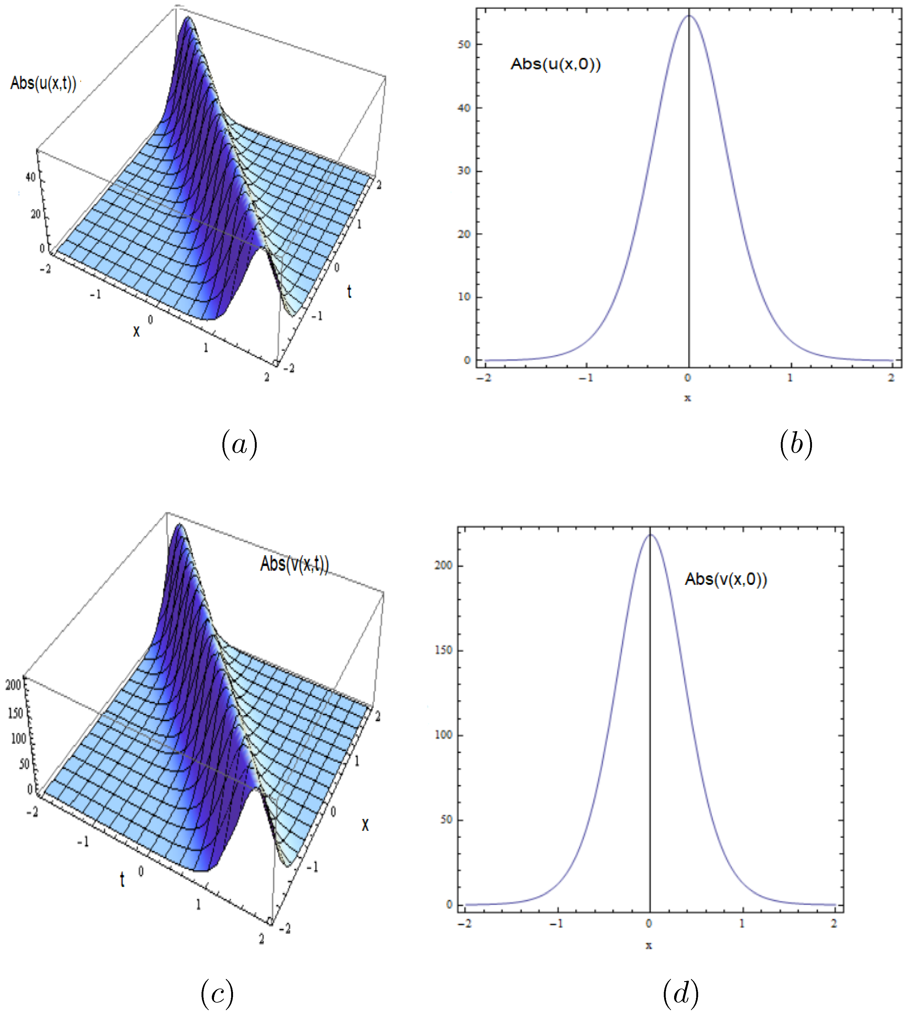
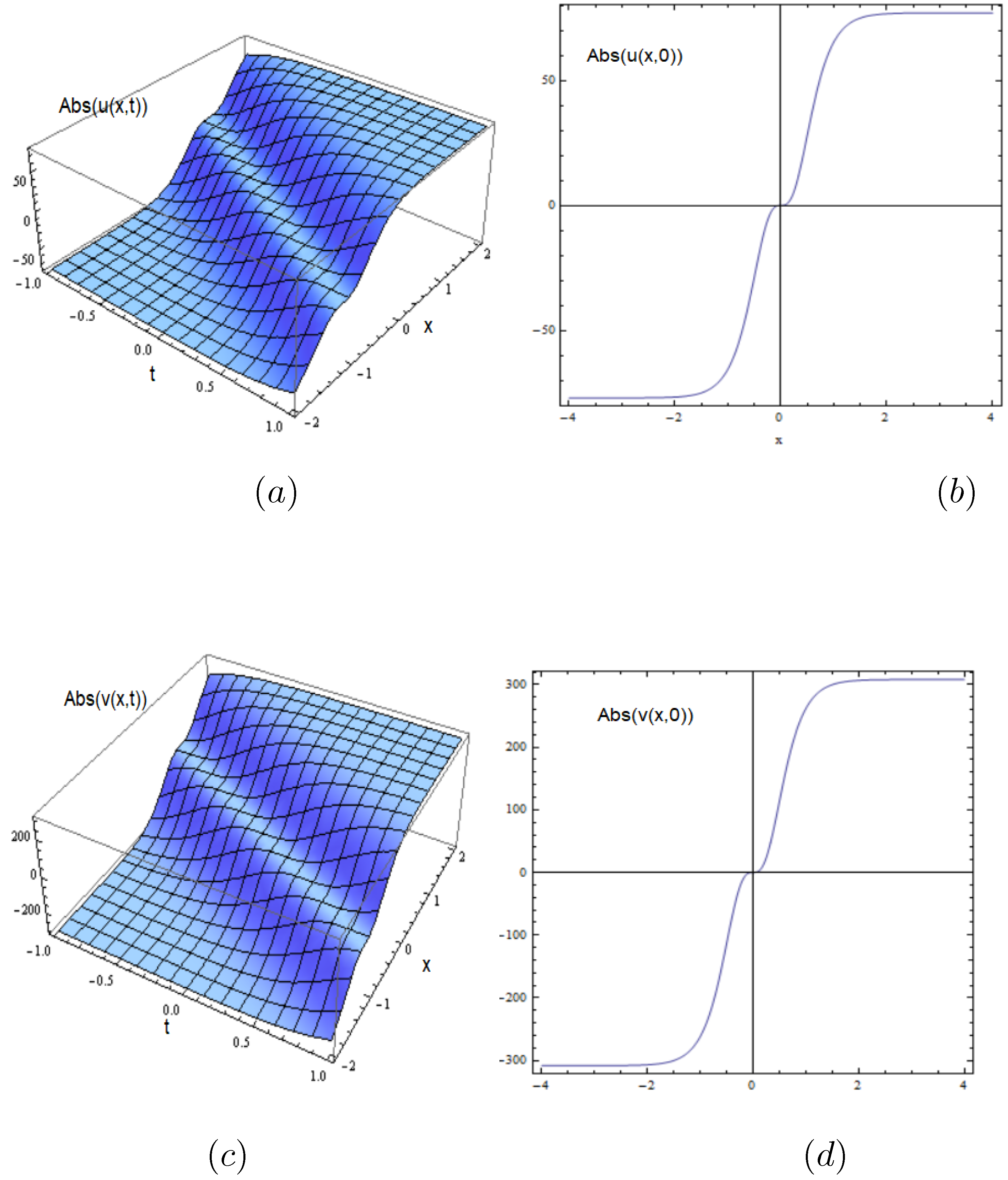
5. Numerical Simulations

In this section, we show the graphs (Figure 1 and Figure 2) of some solutions to Equations (2) and (3). To accomplish this, we choose certain particular values for the obtained parameters of these solutions.

6. Conclusions

The highly dispersive nonlinear complex sixth-order Ginzburg–Landau (CGL) equation in birefringent fibers with Kerr law nonlinearity was studied in this work. Two integration methods were used via the addendum to Kudryashov’s method and the unified Riccati equation expansion method. We found the bright, dark, singular soliton solutions for this model. In future, this work will be extended to fiber Bragg gratings and magneto- optic waveguides. In addition, we will study Equation (1) and the systems (2) and (3) with variable coefficients. Finally, all solutions of this article have been checked using Maple by putting them back into the original equations.

Author Contributions

Methodology, K.A.G.; Software, K.A.G.; Formal analysis, M.E.M.A.; Investigation, M.E.-H.; Data curation, M.E.-H.; Supervision, E.M.E.Z.; Project administration, E.M.E.Z. All authors have read and agreed to the published version of the manuscript.

Funding

This research received no external funding.

Institutional Review Board Statement

Not applicable.

Informed Consent Statement

Not applicable.

Data Availability Statement

All data generated or analyzed during this study are included in this manuscript.

Acknowledgments

The authors thank the anonymous referees whose comments helped to improve the paper.

Conflicts of Interest

The authors declare no conflict of interest.

References

  1. Kudryashov, N.A. One method for finding exact solutions of nonlinear differential equations. Commun. Nonlinear Sci. Numer. Simul. 2012, 17, 2248–2253. [Google Scholar] [CrossRef] [Green Version]
  2. Kudryashov, N.A. A generalized model for description of propagation pulses in optical fiber. Optik 2019, 189, 42–52. [Google Scholar] [CrossRef]
  3. Kudryashov, N.A. Mathematical model of propagation pulse in optical fiber with power nonlinearities. Optik 2020, 212, 164750. [Google Scholar] [CrossRef]
  4. Kudryashov, N.A. Method for finding highly dispersive optical solitons of nonlinear differential equations. Optik 2020, 206, 163550. [Google Scholar] [CrossRef]
  5. Kudryashov, N.A. Highly dispersive optical solitons of the generalized nonlinear eighth-order Schrödinger equation. Optik 2020, 206, 164335. [Google Scholar] [CrossRef]
  6. Kudryashov, N.A. Periodic and solitary waves in optical fiber Bragg gratings with dispersive reflectivity. Chin. J. Phys. 2020, 66, 401–405. [Google Scholar] [CrossRef]
  7. Kudryashov, N.A.; Antonova, E.V. Solitary waves of equation for propagation pulse with powernonlinearities. Optik 2020, 217, 164881. [Google Scholar] [CrossRef]
  8. Abdou, A.; Soliman, A.A.; Biswas, A.; Ekici, M.; Zhou, Q. Dark singular combo opticalsolitons with fractional complex Ginzburg Landau equation. Optik 2018, 171, 463–467. [Google Scholar] [CrossRef]
  9. Akram, G.; Mahak, N. Application of the first integral method for solving (1 + 1) dimensional cubic-quintic complex Ginzburg–Landau equation. Optik 2018, 164, 210–217. [Google Scholar] [CrossRef]
  10. Aranson, I.S.; Krammer, L. The world of the complex Ginzburg- Landau equation. Rev. Mod. Phys. 2002, 74, 99–143. [Google Scholar] [CrossRef] [Green Version]
  11. Biswas, A.; Alqahtani, R.T. Optical soliton perturbation with complex Ginzburg- Landau equationby semi inverse variational principle. Optik 2017, 147, 77–81. [Google Scholar] [CrossRef]
  12. Biswas, A. Chirp-free bright optical solitons and conservation laws for complex Ginzburg- Landauequation with three nonlinear forms. Optik 2018, 174, 207–215. [Google Scholar] [CrossRef]
  13. Biswas, A.; Yildirim, Y.; Yasar, E.; Triki, H.; Alshomrani, A.S.; Ullah, M.Z.; Zhou, Q.; Moshokoa, S.P.; Belic, M. Optical soliton perturbation for complex Ginzburg Landau equation with modified simple equation method. Optik 2018, 158, 399–415. [Google Scholar] [CrossRef]
  14. Cong, H.; Liu, J.; Yuan, X. Quasiperiodic solutions for the cubic complex Ginzburg–Landau equation. J. Math. Phys. 2009, 50, 063516. [Google Scholar] [CrossRef]
  15. García-Morales, V.; Krischer, K. The complex Ginzburg–Landau equation: An introduction. Contemp. Phys. 2012, 53, 79–95. [Google Scholar] [CrossRef]
  16. Lega, J. Traveling hole solutions of the complex Ginzburg–Landau equation: A review. Phys. D Nonlinear Phenom. 2001, 152, 269–287. [Google Scholar] [CrossRef]
  17. Mirzazadeh, M.; Ekici, M.; Sonmezoglu, A.; Eslami, M.; Zhou, Q.; Kara, A.H.; Milovic, D.; Majid, F.B.; Biswas, A.; Belić, M. Optical solitons with complex Ginzburg–Landau equation. Nonlinear Dyn. 2016, 85, 1979–1986. [Google Scholar] [CrossRef]
  18. Neuberger, J.M.; Rice, D.R., Jr.; Swift, J.W. Numerical solutions of a vector Ginzburg Landauequation with a triple well potential. Int. J. Bifurc. Chaos 2003, 13, 3295–3306. [Google Scholar] [CrossRef] [Green Version]
  19. Yıldırım, Y.; Biswas, A.; Kara, A.H.; Ekici, M.; Zayed, E.M.; Alzahrani, A.K.; Belic, M.R. Cubic–quartic optical soliton perturbation and conservation laws with Kudryashov’s law of refractive index. Phys. Lett. A 2020, 384, 126884. [Google Scholar] [CrossRef]
  20. Yıldırım, Y.; Biswas, A.; Ekici, M.; Zayed, E.M.; Khan, S.; Moraru, L.; Alzahrani, A.K.; Belic, M.R. Highly dispersive optical solitons in birefringent fibers with four forms of nonlinear refractive index by three prolific integration schemes. Optik 2020, 220, 165039. [Google Scholar] [CrossRef]
  21. Shwetanshumala, S. Temporal solitons of modified complex Ginzburg- Landau equation. Prog. Electromagn. Res. Lett. 2008, 3, 17–24. [Google Scholar] [CrossRef] [Green Version]
  22. Tien, D.N. A stochastic Ginzburg–Landau equation with impulsive effects. Phys. A Stat. Mech. Its Appl. 2013, 392, 1962–1971. [Google Scholar] [CrossRef]
  23. Zayed, E.M.E.; Alngar, M.E.M.; El-Horbaty, E.; Biswas, A.; Alshomrani, A.S.; Ekici, M.; Yildirm, Y.; Belic, M.R. Optical solitons with complex Ginzburg-Landau equation having a plethora of nonlinearforms with a couple of improved integration norms. Optik 2020, 207, 163804. [Google Scholar] [CrossRef]
  24. Biswas, A.; Yıldırım, Y.; Yaşar, E.; Zhou, Q.; Alshomrani, A.S.; Moshokoa, S.P.; Belic, M. Solitons for perturbed Gerdjikov–Ivanov equation in optical fibers and PCF by extended Kudryashov’s method. Opt. Quantum Electron. 2018, 50, 149. [Google Scholar] [CrossRef]
  25. Li, Z.-L. Periodic wave solutions of a generalized KdV-mKdV equation with higher-order nonlinear terms. Z. Naturforsch. 2010, 56, 649–657. [Google Scholar] [CrossRef]
  26. Biswas, A.; Ekici, M.; Triki, H.; Sonmezoglu, A.; Mirzazadeh, M.; Zhou, Q.; Mahmood, M.; Zaka Ullahi, M.; Moshokoa, S.; Belic, M. Resonant optical soliton perturbation with anti-cubic nonlinearity by extended trial function method. Optik 2018, 156, 784–790. [Google Scholar] [CrossRef]
  27. Zayed, E.M.E.; Alngar, M.E.M.; Biswas, A.; Ekici, M.; Khan, S.; Alshomrani, A.S. Pure-Cubic Optical Soliton Perturbation with Complex Ginzburg–Landau Equation Having a Dozen Nonlinear Refractive Index Structures. J. Commun. Technol. Electron. 2021, 66, 481–544. [Google Scholar] [CrossRef]
  28. Zayed, E.M.E.; Gepreel, K.A.; El-Horbaty, M.; Biswas, A.; Yıldırım, Y.; Alshehri, H.M. Highly Dispersive Optical Solitons with Complex Ginzburg–Landau Equation Having Six Nonlinear Forms. Mathematics 2021, 9, 3270. [Google Scholar] [CrossRef]
  29. Bo, W.-B.; Wang, R.-R.; Fang, Y.; Wang, Y.-Y.; Dai, C.-Q. Prediction and dynamical evolution of multipole soliton families in fractional Schrödinger equation with the PT-symmetric potential and saturable nonlinearity. Nonlinear Dyn. 2022, 111, 1577–1588. [Google Scholar] [CrossRef]
  30. Bo, W.-B.; Wang, R.-R.; Liu, W.; Wang, Y.-Y. Symmetry breaking of solitons in the PT-symmetric nonlinear Schrödinger equation with the cubic–quintic competing saturable nonlinearity. Chaos Interdiscip. J. Nonlinear Sci. 2022, 32, 093104. [Google Scholar] [CrossRef]
  31. Bo, W.-B.; Liu, W.; Wang, Y.-Y. Symmetric and antisymmetric solitons in the fractional nonlinear schrödinger equation with saturable nonlinearity and PT-symmetric potential: Stability and dynamics. Optik 2022, 255, 168697. [Google Scholar] [CrossRef]
  32. Zafar, A.; Shakeel, M.; Ali, A.; Rezazadeh, H.; Bekir, A. Analytical study of complex Ginzburg–Landau equation arising in nonlinear optics. J. Nonlinear Opt. Phys. Mater. 2022, 32, 2350010. [Google Scholar] [CrossRef]
  33. Zafar, A.; Inc, M.; Shakoor, F.; Ishaq, M. Investigation for soliton solutions with some coupled equations. Opt. Quantum Electron. 2022, 54, 243. [Google Scholar] [CrossRef]
  34. Manikandan, K.; Sudharsan, J.B. Manipulating two-dimensional solitons in inhomogeneous nonlinear Schrodinger equation with power-law nonlinearity under -symmetric Rosen–Morse and hyperbolic Scarff-II potentials. Optik 2022, 256, 168703. [Google Scholar] [CrossRef]
  35. Manikandan, K.; Sudharsan, J.B.; Senthilvelan, M. Nonlinear tunneling of solitons in a variable coefficients nonlinear Schrodinger equation with PT-symmetric Rosen–Morse potential. Eur. Phys. B 2021, 94, 122. [Google Scholar] [CrossRef]
  36. Sudharsan, J.B.; Manikandan, K.; Aravinthan, D. Stabilization of solitons in collisionally inhomogeneous higher-order nonlinear media with PT-symmetric harmonic-Gaussian potential with unbounded gain-loss distributions. Eur. Phys. J. Plus 2022, 137, 860. [Google Scholar] [CrossRef]
Figure 1. The numerical simulation of the bright soliton solutions (31) and (32) in 3D and its projection in 2D when a 1 = 1 ,   a 2 = 2 , a 3 = 3 ,   a 4 = 5 ,   a 5 = 2 ,   λ 1 = 4 ,   μ 1 = 3 ,   χ = 4 ,   υ 1 = 5 ,   ζ 1 = 2 ,   K = 5 ,   c 1 = 5 and d 1 = 7 .
Eng 04 00040 g001
Figure 2. The numerical simulation of the dark soliton solutions (54) and (55) in 3D and its projection in 2D when a 1 = 1 ,   a 2 = 2 , a 3 = 3 ,   a 4 = 5 ,   a 5 = 2 ,   λ 1 = 4 ,   μ 1 = 3 ,   χ = 4 ,   υ 1 = 5 ,   ζ 1 = 2 ,   c 1 = 5 , h 1 = 5 ,   h 0 = 2 ,   h 2 = 3 and d 1 = 7 .
Eng 04 00040 g002
Disclaimer/Publisher’s Note: The statements, opinions and data contained in all publications are solely those of the individual author(s) and contributor(s) and not of MDPI and/or the editor(s). MDPI and/or the editor(s) disclaim responsibility for any injury to people or property resulting from any ideas, methods, instructions or products referred to in the content.

