Prediction Model for Optimal Efficiency of the Green Corrosion Inhibitor Oleoylsarcosine: Optimization by Statistical Testing of the Relevant Influencing Factors

Abstract

Optimization and statistical methods are used to minimize the number of experiments required to complete a study, especially in corrosion testing. Here, a statistical Box–Behnken design (BBD) was implemented to investigate the effects of four independent variables (inhibitor concentration [I], immersion time t, temperature ϑ, and NaCl content [NaCl]) based on the variation of three levels (lower, middle, and upper) on the corrosion protection efficiency of the green inhibitor oleoylsarcosine for low-carbon steel type CR4 in salt water. The effects of the selected variables were optimized using the response surface methodology (RSM) supported by the Minitab17 program. Depending on the BBD analytical tools, the largest effects were found for ϑ, followed by [I]. The effect of interactions between these variables was in the following order: [I] and ϑ > t and ϑ > [I] and [NaCl]. The second-order model used here for optimization showed that the upper level (+1) with 75 mmol/L for [I], 30 min for t, and 0.2 mol/L [NaCl] provided an optimal protective effect for each of these factors, while the lower level (−1) was 25 °C for ϑ. The theoretical efficiency predicted by the RSM model was 99.4%, while the efficiency during the experimental test procedure with the best-evaluated variables was 97.2%.

1. Introduction

Oleoylsarcosine (O, Scheme 1) is classified as an N-acylsarcosine derivative that has a high efficiency to inhibit corrosion of low-carbon steel CR4 in 0.1 M NaCl [1]. Organic compounds, such as O, are of increasing interest because of their low cost and potential properties for adsorption to the metal surface [2,3,4]. Furthermore, these derivatives are known to effectively inhibit corrosion and are aerobically and anaerobically biodegradable [5,6,7].

Several parameters affect the corrosion inhibition process, such as the concentration of the used inhibitor [I], the immersion time t of the metal in an anticorrosive solution, the degree of acidity of the surrounding environment, the temperature ϑ, etc. [8,9]. In our recent studies [1,10,11], the classical experimental principle was used to determine the trend of concentration and time dependency of dip coating (immersion time of metal samples). The usual procedure for experimental work, used primarily in research, is to study the effects of changing one factor over time while holding other factors constant. However, these classical methods require a large number of experiments, which consume a lot of materials, such as substrate samples and (inhibitor) solutions, as well as time and effort, thus resulting in high costs [12,13]. In addition, simple trial-and-error methods implemented in such experiments for electrochemical processes cannot easily overcome the complex analytical challenges [14]. To determine the effect of multiple variables on a process, even when there is a complex interaction between them, optimization can help to eliminate the classical methods of experimentation [15]. Before starting such experiments, it is worthwhile to conscientiously plan the experimental work and then follow the developed plan [16]. In this context, there are many recent studies that focus on the application of experimental design and its tools to better explain the effects of different independent variables.

Chemometric tools are used to analyze and optimize the effects of variables and their control on the process [17]. The statistical design of experiment (DOE) is a technique that can be utilized to create an experimental model to reduce the number of tests required compared to the usual experimental methods while taking into account selected or even all relevant parameters in the experiment [17]. In addition to reducing the number of experiments, DOE develops mathematical models that will allow statistical evaluation of the influencing factors and show whether there are significant interactions between the variables in the process. DOE receives the variables as input and gives the result of the experimentation process as output. For optimization strategies there are many mathematical techniques using univariate and multivariate methods [17,18,19]. To avoid errors that may occur in the univariate method when the effect of one variable depends on the level of the other variables involved in the optimization process, the levels of all variables are changed simultaneously, which is processed in multivariate optimization. In multivariate optimization, the first step is to fulfill the screening effect of the studied variables in the fractional factorial design, which depends on the statistical method used in the optimization, to know the main effect of the levels for each variable [20,21,22]. The response surface methodology (RSM) is one of the most important optimization strategies, and it has been shown in many studies to be a very useful tool for application in many areas of industry [23,24,25,26,27,28].

The step after determining the influencing factors that have a significant effect is to apply more complex experimental designs, such as the Box–Behnken design, at three levels [29,30,31]. These may be qualitative factors, such as concentration, temperature, immersion time, etc., or quantitative factors, such as steel type and grade, type of inhibitor, etc. The responses are the independent variables, and their values depend on the level of the factors. BBD is a type of RSM that can be used to determine the best conditions for an optimal result in the experiment. BBD considers an independent quadratic design, and the treatment is located at the midpoint of the edges of the process space and in the center [32]. This technique is designed so that each variable has three levels. There are a number of designs for BBD, and selection of the specific design depends on the number of variables and their levels. The main advantage of the BBD method is the smaller number of experiments compared to other response surface designs, e.g., the central composite design [18,33].

In the present work, the BBD method was used to optimize the influence of four independent variables affecting the protection of steel CR4 against corrosion in salt water. The aim was to determine the optimum protective effect that can be achieved using the examined levels of the selected factors. The selected independent variables and their denomination were the concentration of inhibitor [I], the immersion time t of the steel samples in the anticorrosive inhibitor stock solution, the temperature ϑ of the test solution, and the NaCl content [NaCl] in the testing solution. Each independent variable had three levels (low, mid, and upper) and was designed as coded value (−1, 0, and +1). The dependent variable (objective function) to be determined was the efficiency of the inhibitor to reduce the current density and to achieve the best protection.

2. Materials and Methods

2.1. Metal Samples, Inhibitor, and Experimental Setup

Low-carbon steel type CR4, which corrodes relatively quickly at ambient environment without protection, was tested against corrosion in salt water with three different NaCl contents (0.05, 0.1, and 0.2 M). The single steel sheets were laser-cut in the dimensions 25 × 25 × 1 mm and delivered without further treatment by the supplier (Janssen CNC-Blechbearbeitungs GmbH, 65604 Elz, Germany). The chemical composition was analyzed by optical emission spectroscopy (Vario Lab, Belec Spektrometrie Opto-Elektronik GmbH, 49124 Osnabrück, Germany). The result of the metal analysis was in line with the standard range of this steel type (CR4, also denominated as DC01- [1,34]).

Proper preparation, such as grinding, cleaning, drying of metal samples, and coating with the selected inhibitor, was carried out before testing. Details can be found in [1,11,12]. Briefly, the specifics of this investigation were as follows. After grinding according to DIN EN ISO 9227:2006 and DIN EN ISO 1514:2005-02 [35,36] with silicon carbide paper (120 and 220, WS FLEX 18c waterproof, HERMES, Hamburg, Germany), the samples were cleaned ultrasonically in isopropanol (10 min) and dried with pressurized air. Subsequently, they could be used immediately for immersion in the inhibitor solutions or stored at 60 °C for slightly later use. The final step prior to corrosion testing was coating with an inhibitor at three different concentrations [I] (25, 50, and 75 mmol/L in toluene) and at three different duration times t (1, 10, and 30 min). According to our previous studies of N-acyl-sarcosine derivatives [1,11], the most effective inhibitor oleoylsarcosine (O) was used.

Potentiodynamic polarization (Galvanostate Wenking, working electrode 1 cm², thermostated cell, LPG03 system, Bank Electronic—Intelligent Controls GmbH, 35415 Hessen, Germany) was carried out following previous studies [1,10,11] to test the inhibitor O and find the optimum corrosion protection for steel CR4 according to the experimental design. This included variation of the variables [I], t, ϑ, and [NaCl], as mentioned above. Prior to any measurement, the open circuit potential (OCP) was equilibrated at free potential. The pH value was controlled to be constant at 6.5 ± 0.5 (EL20/EL2, Toledo Group, Zurich, Switzerland). Polarizations were recorded in duplicate at ±150 mV with respect to the OCP and a scan speed of 0.5 mV/s.

2.2. Experimental Design and Optimization

Design of experiments (DOE) involves subjecting certain experimental parameters, i.e., variables, to an organized treatment using a designed measurement matrix in order to obtain appropriate responses. Each experiment has one or more variables that represent an input to the DOE (A, B, C, etc.), which is then converted to a corresponding output (Y). After obtaining reasonable results from this experimental design and following proper analysis, the optimal experiment can be planned. All DOE techniques are nontraditional methods. Independent variables that represent effective combinations of each other are determined so that the tests can be carried out statistically in a limited number. The Box–Behnken design (BBD) is one such technique that reduces the required number of experiments while maintaining the accuracy of the results. The type of design depends on the levels used for the variables. A two-level matrix includes only a lower and upper limit (−1 and +1), while a three-level matrix includes an additional midpoint (−1, 0, and +1). For each classical experimental procedure, a certain number of experiments is required, which can be calculated from the number of variables and levels according to Equation (1):

$$\mathrm{S}=l^k$$

(1)

where S is the number of experiments, l the number of levels, and k the number of variables.

In the present work, the number of experiments required in a conventional study with four variables and three levels each according to Equation (1) would have been as follows: 3⁴ = 81. However, the required number was minimized with BBD. The independent variables with their levels were performed in coded values, as summarized in

Table 1. The four independent variables with their levels performed with coded values.

No.	Variable Code	Selected Variable	Coded Level
			−1	0	+1
1	A	Inhibitor concentration [I] (mmol/L)	25	50	75
2	B	Immersion time t (min)	1	10	30
3	C	Temperature ϑ (°C)	25	40	55
4	D	NaCl content [NaCl] (mol/L)	0.05	0.1	0.2

. The orthogonal three-level matrix for four variables with three levels each according to BBD therefore resulted in only 27 runs, as shown in

Table 2. Three-level matrix for four variables (A, B, C, and D) and three levels (−1, 0, and +1) according to BBD with resulting 27 single experiments.

Coded Value
No.	A	B	C	D
1	−1	−1	0	0
2	−1	+1	0	0
3	+1	−1	0	0
4	+1	+1	0	0
5	0	0	−1	−1
6	0	0	−1	+1
7	0	0	+1	−1
8	0	0	+1	+1
9	−1	0	0	−1
10	−1	0	0	+1
11	+1	0	0	−1
12	+1	0	0	+1
13	0	−1	−1	0
14	0	−1	+1	0
15	0	+1	−1	0
16	0	+1	+1	0
17	−1	0	−1	0
18	−1	0	+1	0
19	+1	0	−1	0
20	+1	0	+1	0
21	0	−1	0	−1
22	0	−1	0	+1
23	0	+1	0	−1
24	0	+1	0	+1
25	0	0	0	0
26	0	0	0	0
27	0	0	0	0

.

The main objective of the DOE application is to optimize the experimental process and predict the maximum response Y depending on the selected variables and levels with a minimum number of experiments. There are many computer-aided optimization methods for DOE, but RSM is one of the most effective [37,38]. RSM combines statistical and mathematical techniques that are useful in developing, improving, and optimizing processes. The first aim in RSM is to find the optimal response Y. The second objective is to understand how Y changes in a particular direction by a graphical adaptation. Here, the efficiency of the inhibitor is the response variable expressed as a function of four independent variables, as shown in Equation (2) [37]:

$$\mathrm{Y}=f\left(A,B,C,D\right)+\epsilon$$

(2)

where A, B, C, and D are the variables, and ε is the experimental error.

RSM starts with a first-order model function if the response is a linear function of the independent variables. Here, the first-order model can be expressed as Equation (3):

$$\mathrm{Y}={\beta }_0+{\beta }_{1}A+{\beta }_{2}B+{\beta }_{3}C+{\beta }_{4}D+\epsilon$$

(3)

where β is the respective regression coefficient.

If the response surface has a curvature, then a second-order model should be used, given in Equation (4):

$$\begin{array}{l}\mathrm{Y}={\beta }_0+{\beta }_{1}A+{\beta }_{2}B+{\beta }_{3}C+{\beta }_{4}D\\ \hspace{1em}\hspace{0.17em}+{\beta }_{11}{A}^2+{\beta }_{22}{B}^2+{\beta }_{33}{C}^2+{\beta }_{44}{D}^2\\ \hspace{1em}\hspace{0.17em}+{\beta }_{12}AB+{\beta }_{13}AC+{\beta }_{14}AD+{\beta }_{23}BC+{\beta }_{24}BD+{\beta }_{34}CD+\epsilon \end{array}$$

(4)

In this work, the second-order model for RSM was used to identify all possible effects on the process. RSM was applied using Minitab 17 to perform 27 experiments and determine the responses based on the proposed predictive mode.

3. Results and Discussion

3.1. Experimental Corrosion Protection Efficiencies According to the BBD Matrix

Polarization measurements were carried out according to the aforementioned BBD matrix to analyze the effects of the four selected variables on the protection efficiency. The result of these 27 experimental runs is given in

Table 3. Efficiency results of the 27 experiments according to the BBD matrix, including the coded and real values (compare Table 1).

Coded Value					Real Value				Efficiency %
No.	A	B	C	D	A	B	C	D
1	−1	−1	0	0	25	1	40	0.1	85.20 ± 4.1
2	−1	+1	0	0	25	30	40	0.1	77.99 ± 8.9
3	+1	−1	0	0	75	1	40	0.1	66.77 ± 2.1
4	+1	+1	0	0	75	30	40	0.1	69.87 ± 3.6
5	0	0	−1	−1	50	10	25	0.05	89.11 ± 0.6
6	0	0	−1	+1	50	10	25	0.2	92.06 ± 0.8
7	0	0	+1	−1	50	10	55	0.05	39.94 ± 0.2
8	0	0	+1	+1	50	10	55	0.2	37.86 ± 2.5
9	−1	0	0	−1	25	10	40	0.05	70.05 ± 8.0
10	−1	0	0	+1	25	10	40	0.2	52.40 ± 6.1
11	+1	0	0	−1	75	10	40	0.05	85.57 ± 1.0
12	+1	0	0	+1	75	10	40	0.2	74.59 ± 4.8
13	0	−1	−1	0	50	1	25	0.1	92.86 ± 0.1
14	0	−1	+1	0	50	1	55	0.1	50.15 ± 8.3
15	0	+1	−1	0	50	30	25	0.1	91.96 ± 1.0
16	0	+1	+1	0	50	30	55	0.1	41.80 ± 9.7
17	−1	0	−1	0	25	10	25	0.1	91.98 ± 1.6
18	−1	0	+1	0	25	10	55	0.1	54.26 ± 7.9
19	+1	0	−1	0	75	10	25	0.1	94.35 ± 0.5
20	+1	0	+1	0	75	10	55	0.1	46.03 ± 4.1
21	0	−1	0	−1	50	1	40	0.05	86.46 ± 2.3
22	0	−1	0	+1	50	1	40	0.2	80.63 ± 0.2
23	0	+1	0	−1	50	30	40	0.05	76.51 ± 3.9
24	0	+1	0	+1	50	30	40	0.2	73.55 ± 4.6
25	0	0	0	0	50	10	40	0.1	74.23 ± 0.5
26	0	0	0	0	50	10	40	0.1	74.23 ± 0.5
27	0	0	0	0	50	10	40	0.1	74.23 ± 0.5

.

For the next step in optimization of the variables’ influence, including their levels, RSM was applied on the data outlined in Table 3. The tools used to analyze and optimize the process are given in the following sections: general effects of variables (see Section 3.2.), response plot (see Section 3.3.), normal probability distribution (see Section 3.4.), and optimization by RSM (see Section 3.5.).

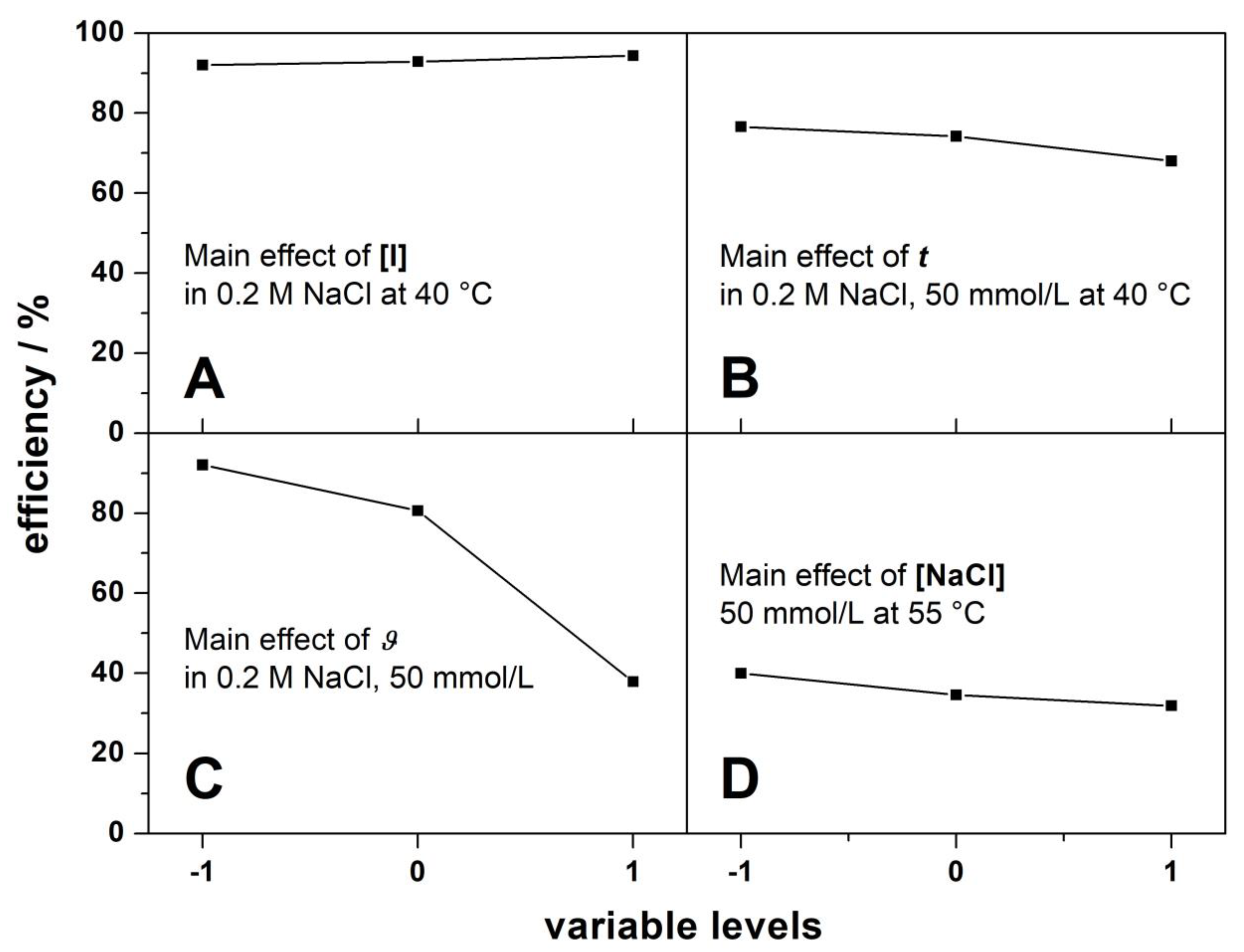
3.2. General Effects of the Variables and Their Levels

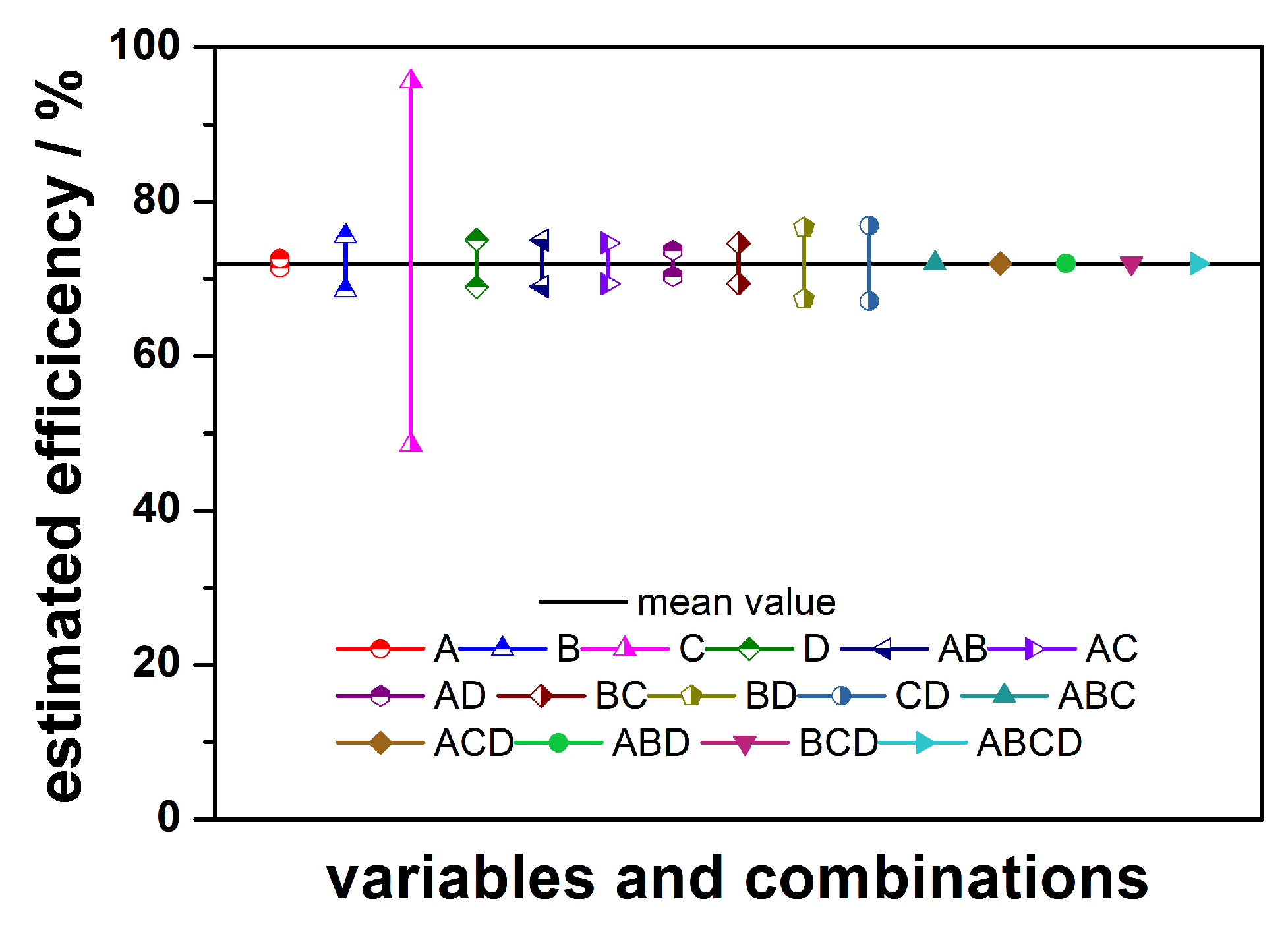
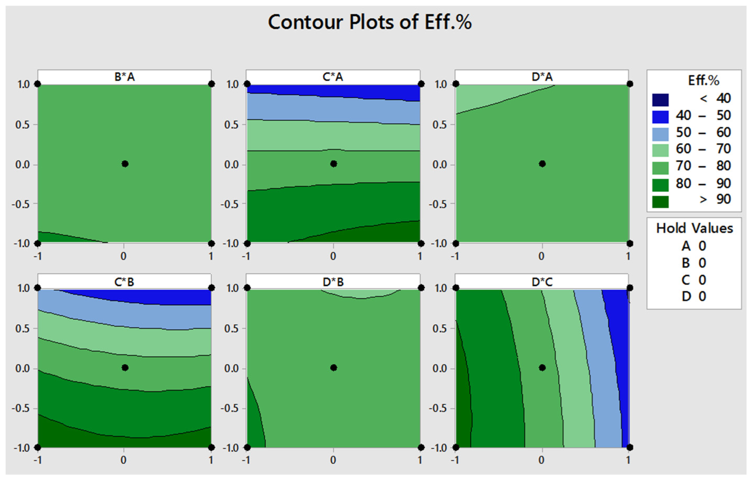
Before starting the optimization process, it is important to outline the main effects of each variable depending on its level (−1, 0, and +1)). Figure 1 displays the main effect diagrams (based on results of

Table 4. Normal probability calculations.

Variable/ Interaction	Estimated Effect Ef	Rank I	Probability (Pi) = 100(I − 0.5)/10
C	47.046	1	5
CD	9.805	2	15
BD	9.244	3	25
B	6.952	4	35
D	6.091	5	45
AB	6.021	6	55
AC	5.300	7	65
BC	5.186	8	75
AD	3.335	9	85
A	1.158	10	95
Mean	10.014	-	-

), which show the response of each variable as it changes according to the given level, for the current corrosion protection process with the selected inhibitor O. The following observations can be derived from Figure 1.

The protection efficiency gradually increased as the inhibitor O concentration increased, reaching an optimum of 94% at the upper level (+1, Figure 1A). For the remaining variables t, ϑ, and [NaCl] (Figure 1B–D), the highest efficiency was achieved at their respective lower levels (−1). Considering all changes in the individual main effect diagrams, it can be noticed that the temperature (Figure 1C), had the greatest influence. The change in the efficiency was significantly more pronounced when switching between the levels than for any other variable (Figure 1C). The overall least effect was recorded for the salt content with efficiencies around 40% (Figure 1D).

This general overview only gives a quick indication of the behavioral effect of the tested independent variables. For a more in-depth analysis, BBD tools, such as response graphs, normal probability distribution, and interaction effect graphs, were used.

3.3. Response Plot

The result of the implantation runs in the BBD experimental design are shown in the response table (see Supporting Information S1). Each determined efficiency value represents the average of two independent experiments to ensure reproducibility. With the plot of the response graph in Figure 2, the individual and interactive effects of the variables on the process can be easily examined. The effect of the variables and their levels on efficiency is represented as E_f, which was obtained by the higher (l_H) and lower (l_L) values for each factor and interaction in the response table (see Supporting Information S1). The response graph (Figure 2) represents the estimated impact. Therefore, it is a valuable tool that uses the absolute impact to analyze the effect of factors on the efficiency of the process.

From the response graph (Figure 2), it is clear that the temperature had the greatest influence in reducing corrosion in the presence of inhibitor O, with E_f C = 47 (half-filled triangles up, magenta). This is consistent with the result of the main effect plot in Figure 1. The interactions between temperature and [NaCl], depicted as CD, ranked second for the influence on the process, along with the immersion time and [NaCl], depicted as BD (E_f = 9 for both, half-filled circles in blue and half-filled pentagons in dark yellow, respectively). The immersion time, depicted as B, followed on rank 3 (E_f = 7, blue, half-filled triangles up), while both the NaCl content and the interaction between [I] and t, depicted as D and AB, respectively, were rank 4 (E_f = 6 for both, green half-filled diamonds and dark blue half-filled triangles left, respectively). Rank 5 was shared by the interactions between AC and BC, each with an effect of 5 (light purple half-filled triangles right and brown half-filled diamonds, respectively). The interaction between inhibitor concentration and NaCl content results came in at rank 6 with E_f AD = 3 (dark purple half-filled diamonds). In the last place of individual and combined two-factor interactions was the inhibitor concentration, depicted as A, with E_f of only = 1 (red half-filled circles), which meant that a change of inhibitor O to higher concentrations did not have a great influence on the response (and therefore the efficiency of corrosion protection). Interactions between three and four factors had the same value for the mean efficiency of the process, which in the end had no detectable effects on corrosion protection (Figure 2).

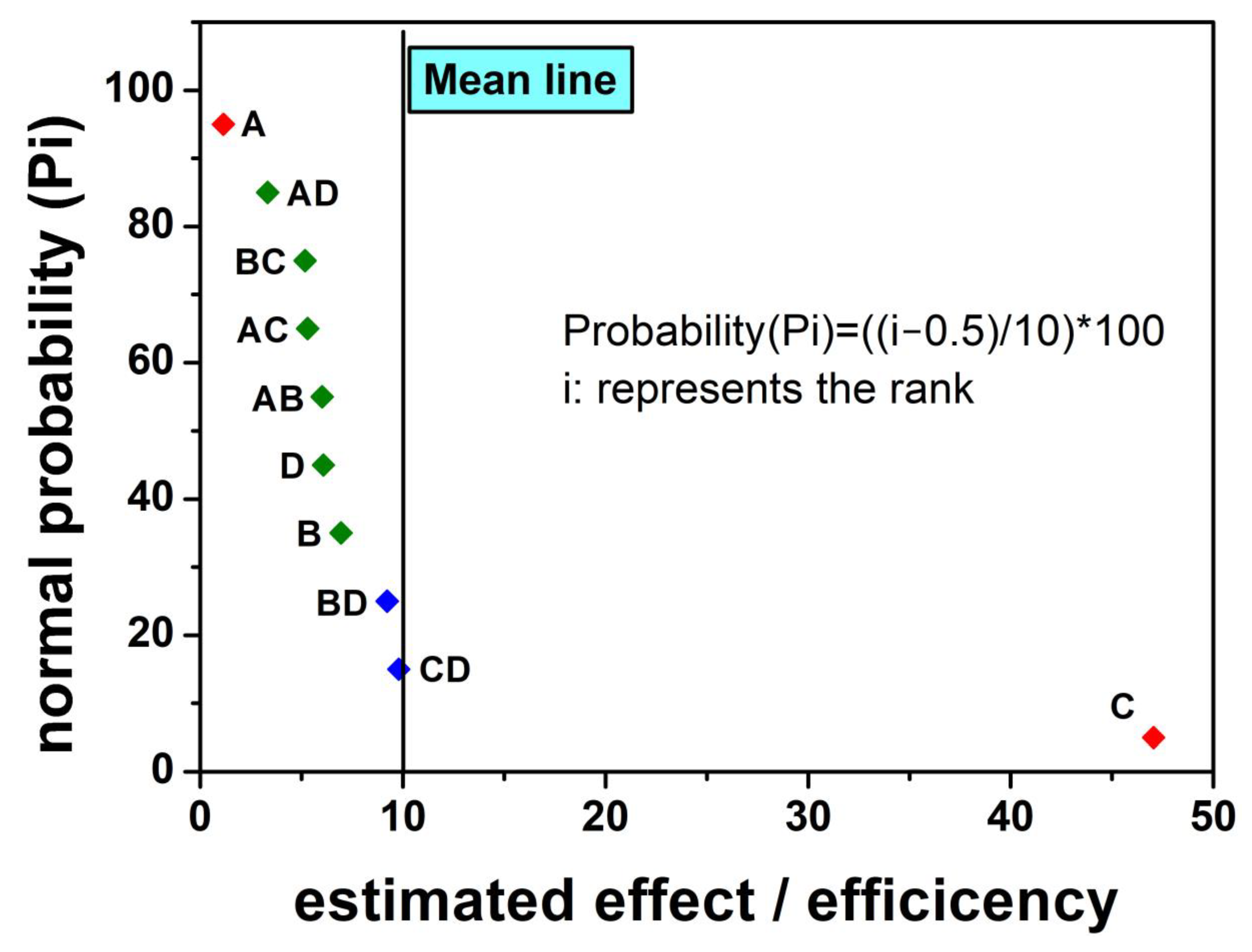
3.4. Normal Probability Plot

The results reviewed in the response graph (Figure 2) clearly indicated that some variables and interactions had a greater effect than others. To ensure that these effects were real and did not just occur by chance, a normal probability representation was applied. Calculations required to plot the normal probability are summarized in Table 4. The probability represents how far the variables and their respective interactions affected the corrosion protection.

The estimated effect of the variables and the interactive effects yielded the normal probability data given in Table 4 according to the order from maximum to minimum value. Figure 3 shows the normal probability diagram, which indicates which factors and interactions had a significant influence on the protection efficiency and which were rather insignificant. The effective value is based on the distance of the data point (colored diamond) from the mean line, with the effect being greater the further it is from it. The red diamonds refer to the variables and combinations that have the strongest effect, the green ones still have a good to moderate effect, while the blue ones indicate insignificant effects. From this, it can be clearly deduced that the temperature (C) and the inhibitor concentration (A) had the greatest influence on the efficiency (red diamonds) as they are most distant from the mean line. Accordingly, the interaction effects AB, AC, BC, and AD (green diamonds) also had good effects. The individual variables of the immersion time (B) and the NaCl content (D), shown as green diamonds, still indicated a good to moderate effect. The interactive effects between ϑ and [NaCl] (CD) as well as immersion time and [NaCl] (BD) (blue diamonds) had an insignificant effect as they are very close to the indicated mean line.

The normal probability distribution in Figure 3 clearly shows that the concentration of inhibitor O had a high effect on protection, while in the response graph in Figure 2, it showed a lower effect compared to the other variables and interactions. As mentioned before, the normal probability shows the actual impact of the factors affecting the process rather than the random impact. This also explains why some factors had a greater influence in the response graph than in the normal probability distribution and vice versa. For this reason, it was reasonable to use both methods for data analysis in the current study.

3.5. Optimization

The RSM (response surface methodology) was used here to determine the maximum protection efficiency for inhibitor O in accordance with the selected factors and their chosen levels. Optimization was implemented to statistically design the combinations, determine the coefficient by fitting the experimental results to the response function, predict the response according to the fitted model, and finally check the fit of the designed model.

3.5.1. Implementation of the Empirical Model

Here, the second-order model of Equation (4) was used, with only the double interaction effect included in the regression model. Regression coefficients were obtained using Minitab 17 software and are summarized in

Table 5. Obtained regression coefficients of the optimization model according to Equation (4).

No.	Coefficient	Coefficient Obtained	Symbol
1	Constant	74.23	ß0
2	A	0.44	ß1
3	B	−2.53	ß2
4	C	−23.52	ß3
5	D	−3.05	ß4
6	AA	−0.23	ß11
7	BB	2.86	ß22
8	CC	−6.07	ß33
9	DD	−1.52	ß44
10	AB	2.58	ß12
11	AC	−2.65	ß13
12	AD	1.67	ß14
13	BC	−1.86	ß23
14	BD	0.72	ß24
15	CD	−1.26	ß34

(see Supporting Information S2).

Using the regression coefficients listed in

Table 6. The actual experimental efficiency and the efficiency predicted by the model according to Equation (4).

Experiment No.	Experimental Efficiency [%]	Predicted Efficiency [%]	Error [%]
1	85.20	81.52	2.59
2	77.99	71.30	4.72
3	66.77	77.25	7.41
4	69.87	77.34	5.28
5	89.11	91.95	2.00
6	92.06	88.37	2.60
7	39.94	47.42	5.28
8	37.86	38.81	0.67
9	70.05	76.74	4.73
10	52.40	67.32	10.55
11	85.57	74.29	7.97
12	74.59	71.54	2.15
13	92.86	95.21	1.66
14	50.15	51.88	1.23
15	91.96	93.87	1.35
16	41.80	43.09	0.91
17	91.98	88.36	2.55
18	54.26	46.61	5.40
19	94.35	94.54	0.13
20	46.03	42.20	2.70
21	86.46	81.86	3.25
22	80.63	74.33	4.45
23	76.51	75.36	0.81
24	73.55	70.70	2.01
25	74.23	74.23	0
26	74.23	74.23	0
27	74.23	74.23	0

and the regression equation generated by the program (see Supporting Information S3), the empirical model in Equation (4) can be rewritten as follows:

Predicted efficiency % = 74.23 + 0.44 × A − 2.53 × B −23.53 × C − 3.05 × D − 0.23 × A² + 2.86 × B² − 6.07 × C² −
1.52 × D² + 2.58 × AB − 2.65 × AC + 1.67 × AD − 1.86 × BC + 0.72 × BD − 1.26 × CD

(5)

The determination of multiple coefficients (R²) for the proposed predictor model yielded 89.2%, which meant that only 10.8% was not considered by the proposed model, indicating a good acceptance of the model used in this study. The actual experimental efficiency, the predicted efficiency resulting from the application of the empirical model, and the error resulting from the difference between them are given in Table 6.

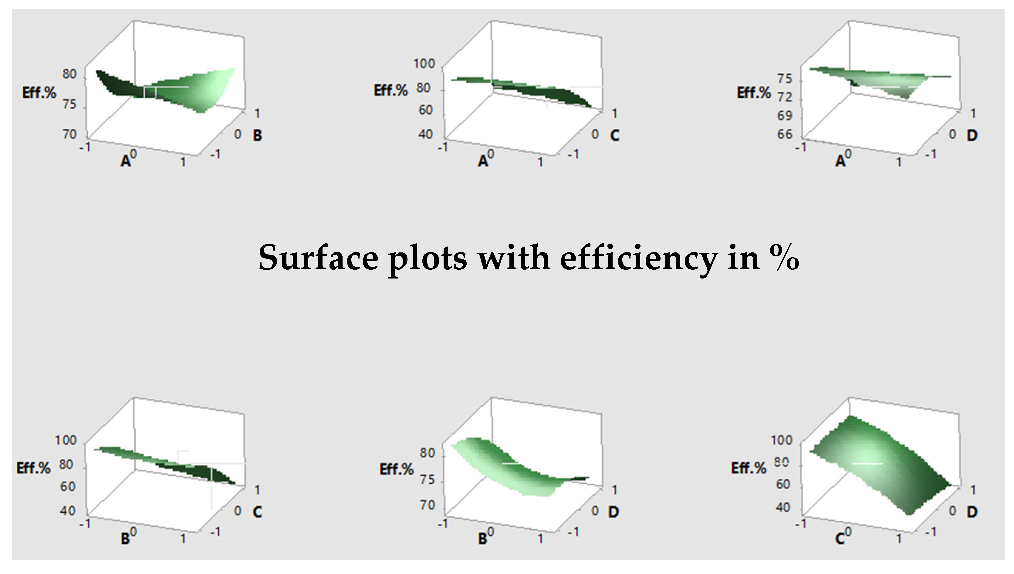
3.5.2. Statistical Simulation of the RSM

The simulation of RSM was carried out to understand the changes in response according to a particular direction by adjusting the selected variables. The response surface was plotted graphically in 3D and 2D (Figure 4 and Figure 5, respectively). In the response surface plot, only two variables could be included in the diagram, so the other two factors were placed at the middle level (0 level). Figure 4 shows a 3D plot of efficiency for each of the two variables changing from a lower to a higher level.

Contour plots were used to make the results of the response surface more visible and understandable, as shown in Figure 5. The contour plot was a 3D plot created for each two pairs of factors while keeping the others factors at the middle level. If the inhibitor concentration (A) versus the immersion time (B) changed from the lower to the upper level while C and D remained at the middle level, this essentially resulted in an efficiency of up to 80% and only partly up to 90% when A and B were at the lower level (Figure 5B*A). The efficiency was around 90% when the levels of C and A moved from lower (−1) to middle (0) and less than 50% at the (+1) level (Figure 5C*A). No significant effect could be detected for factors D and A from (−1) to (0) with 70–80% and only a decrease to 60% towards the upper level, corresponding to an increased NaCl content (Figure 5D*A). For the combination of temperature C and immersion time B, a continuous decrease from up to 90% at level −1 to as low as 40% at level +1 was observed (Figure 5C*B). For factors D and B, there was an efficiency of around 90% at the −1 levels, which decreased extensively to 80% to the 0 and +1 levels (Figure 5D*B). The last surface response plot (Figure 5D*C) showed an interesting behavior of temperature (C) and NaCl content (D) as the effect of C was more controlled than D. For factor C, the effect on D was stable at all levels as it moved from −1 to 0, with an efficiency of around 80–90%, while it dropped to 40% when C moved to the upper level (+1), with the effect of D remaining stable throughout (Figure 5D*C).

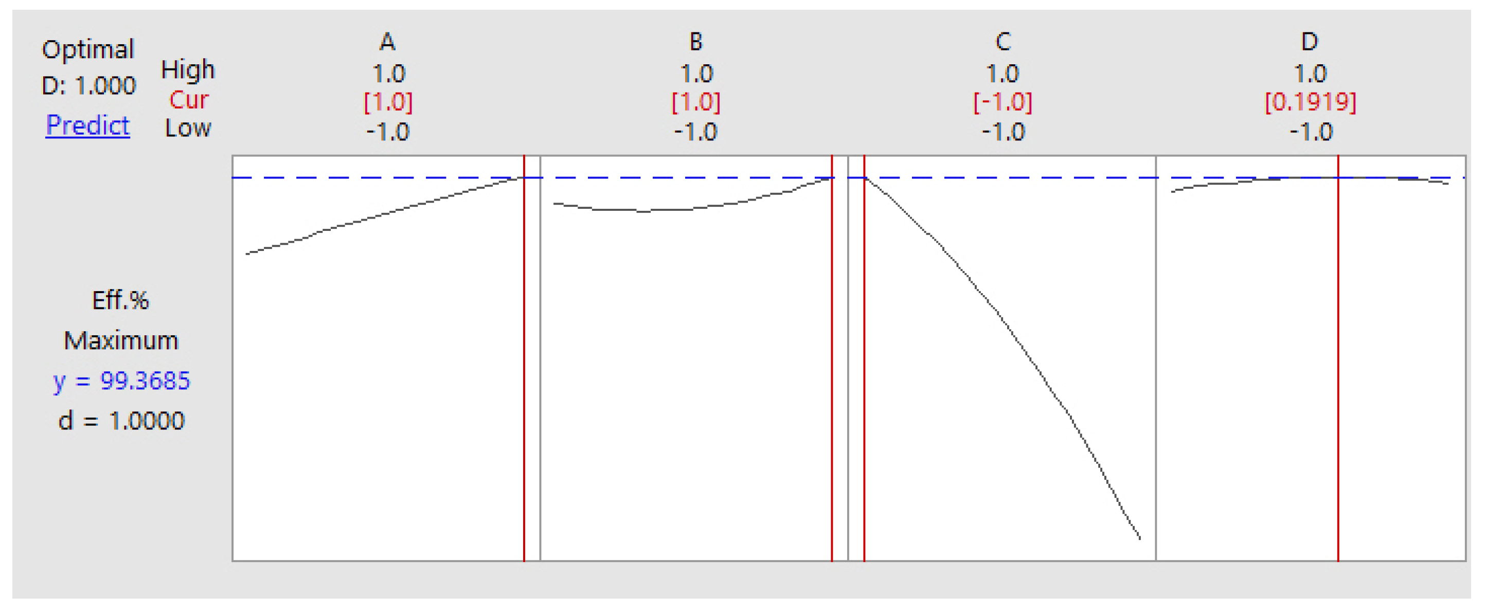
3.5.3. Find the Optimal Levels for Best Prediction

To find the best values for the levels that provide optimal efficiency in the current protection process with compound O, the proposed predicted model was used and applied by Minitab17. Using the software, it was determined that the upper level (+1) was optimal for inhibitor concentration (A) and immersion time (B), while the lower level (−1) was better for the temperature factor (C, see Figure 6). For the NaCl content (D), the value was 0.1919, which is approximately 0.2 (real value = 0.2 M) and thus corresponded to the upper level. Therefore, the most appropriate levels for the selected factors could be determined by the prediction model used for A (+1), B (+1), C (−1), and D (+1). Moreover, this series was not included in the BBD matrix, which is a successful indicator for the model proposed in this study. The overall predicted efficiency depending on the regression equation was 99.4% (see Figure 6).

By substituting the obtained values and according levels from the RSM by Minitab17 for each tested variable into Equation (6), the optimal value of efficiency can be predicted as follows:

Predicted efficiency % = 74.23 + 0.44 × (1) − 2.53 × (1) −23.53 × (−1) − 3.05 × (0.1919) − 0.23 × (1)² + 2.86 × (1)² −
6.07 × (−1)² −1.52 × (0.1919)² + 2.58 × (1 × 1) − 2.65 × (1 × −1) + 1.67 × (1 × 0.1919) − 1.86 ×
(1 × −1) + 0.72 × (1 × 0.1919) − 1.26 × (−1 × 0.1919) = 99.4

(6)

The optimal protective effect predicted theoretically by RSM supported using Minitab17 was 99.4% according to the following combination of levels: A = 75 mmol/L (+1), B = 30 min (+1), C = 25 °C (−1), and D = 0.2 M NaCl (+1). Thus, the predicted efficiency was higher than the maximum experimental efficiency of 94.4% obtained in experiment No. 19 (for details, see Table S1 and Supporting Information S3). Even though the predicted combination was not included in the 27 single designed tests determined in the matrix, it was essential to confirm it experimentally. In Figure 7, the anodic and cathodic polarization for experiment No. 19 (red) is displayed, together with the predicted and experimentally confirmed one (optimum in blue) in comparison to the unprotected steel CR4 as reference (black).

The experimentally confirmation, including the predicted combination of the levels (+1, +1, −1, and +1), was performed and resulted in a 97.2% efficiency. In comparison to the theoretical value of 99.4%, this results is an error of 2.2%, indicating high confirmation and acceptance of the proposed predictive model.

4. Conclusions

In this work, the efficiency of the compound oleoylsarcosine in inhibiting corrosion of steel type CR4 in aqueous solution with different NaCl contents was investigated. Furthermore, the variables that have the greatest influence on corrosion protection, such as inhibitor concentration, immersion time, temperature, and NaCl content, were evaluated accordingly. The individual tests were performed based on a design of experiments using the Box–Behnken design (BBD) technique. The optimization process was carried out using the response surface methodology (RSM) supported by the program Minitab17 to determine the optimal efficiency of the process according to selected variables and their respective levels. The obtained results showed that the BBD technique used here is a good systematic control tool to explore the process of corrosion protection by inhibitors. In this context, BBD is suitable as a very flexible means of representing changing environmental conditions, allowing the variables or their limits to be changed and controlled. The data obtained explain how the factors tested affect the process, with temperature having the greatest influence, followed by inhibitor concentration. The possible interactions between the selected variables was also examined in BBD, with the interaction of inhibitor concentration and temperature (AC), immersion time and temperature (BC), and inhibitor concentration and NaCl content (AD) having larger effects than all others.

In the subsequent optimization, the upper level (+1) proved to be the better limit for the inhibitor concentration (A), immersion time (B), and NaCl content (D), while the lower level (−1) was found to be optimal for the temperature (C). The RSM acceptance was up to 89.2% when using the program Minitab 17 to determine the predicted response in comparison to the experimental results.

The highest efficiency obtained on the basis of the experimental design was up to 94% in one test with the following combination of variables and levels: A +1, B 0, C −1, and D 0. The optimal efficiency theoretically predicted by RSM was 99.4% with the combination A +1, B +1, C −1, and D +1, which in turn was not included in the experimental design matrix. In summary, the error between the theoretical and experimental results of the optimum efficiency was only 2.2%, indicating good confirmation and acceptance of the proposed prediction model.

References

1. Kaskah, S.E.; Pfeiffer, M.; Klock, H.; Bergen, H.; Ehrenhaft, G.; Ferreira, P.; Gollnick, J.; Fischer, C.B. Surface protection of low carbon steel with N-acyl sarcosine derivatives as green corrosion inhibitors. Surf. Interfaces 2017, 9, 70–78. [Google Scholar] [CrossRef]
2. Rahim, A.A.; Kassim, J. Recent development of vegetal tannins in corrosion protection of iron and steel. Recent Pat. Mater. Sci. 2008, 1, 223–231. [Google Scholar] [CrossRef]
3. Zhao, L.; Teng, H.K.; Yang, Y.S.; Tan, X. Corrosion inhibition approach of oil production systems in offshore oilfields. Mater. Corros. 2004, 9, 684–688. [Google Scholar] [CrossRef]
4. Moyo, F.; Tandlich, R.; Wilhelm, B.S.; Balaz, S. Sorption of hydrophobic organic compounds on natural sorbent and organoclays from aqueous and non-aqueous solutions: A mini-review. Int. J. Environ. Res. Public Health 2014, 11, 5020–5048. [Google Scholar] [CrossRef] [PubMed] [Green Version]
5. Lanigan, S. Final Report on the Safety Assessment of Cocoyl Sarcosine, Lauroyl Sarcosine, Myristoyl Sarcosine, Oleoyl Sarcosine, Stearoyl Sarcosine, Sodium Cocoyl Sarcosinate, Sodium Lauroyl Sarcosinate, Sodium Myristoyl Sarcosinate, Ammonium Cocoyl Sarcosinate, and Ammonium Lauroyl Sarcosinate. Int. J. Toxicol. 2001, 20, 1–14. [Google Scholar] [PubMed]
6. Frignani, A.; Trabanelli, G.; Wrubl, C.; Mollica, A. N-Lauroyl sarcosine sodium salt as a corrosion inhibitor for type 1518 carbon steel in neutral saline environments. NACE Int. Corros. 1996, 52, 177–182. [Google Scholar] [CrossRef]
7. Salensky, G.A.; Cobb, M.G.; Everhart, D.S. Corrosion-Inhibitor Orientation on Steel. Ind. Eng. Chem. Prod. Res. Dev. 1986, 25, 133–140. [Google Scholar] [CrossRef]
8. Popov, B.N. Corrosion Engineering Principles and Solved Problems; Elsevier, B.V.: Amsterdam, The Netherlands, 2015. [Google Scholar]
9. Sastri, V.S. Challenges in Corrosion: Cost, Causes, Consequences, and Control; John Wiley: Hoboken, NJ, USA, 2015. [Google Scholar]
10. Kaskah, S.E.; Ehrenhaft, G.; Gollnick, J.; Fischer, C.B. Concentration and coating time effects of N-acyl sarcosine derivatives for corrosion protection of low-carbon steel CR4 in salt water—Defining the window of application. Corros. Eng. Sci. Technol. 2019, 3, 216–224. [Google Scholar] [CrossRef]
11. Kaskah, S.E.; Ehrenhaft, G.; Gollnick, J.; Fischer, C.B. N-b-Hydroxyethyl Oleyl Imidazole as Synergist to Enhance the Corrosion Protection Effect of Natural Cocoyl Sarcosine on Steel. Corros. Mater. Degrad. 2022, 3, 536–552. [Google Scholar] [CrossRef]
12. Nist, N.I. Comparisons of response surface design. In NIST/SEMATECH e-Handbook of Statistical Methods; United States Department of Commerce: Washington, DC, USA, 2012. [Google Scholar] [CrossRef]
13. Penteado, R.B.; Hag Ui, J.C.; Faria, J.C.; Ribeiro, M.V. Application of Taguchi Method in process improvement of turning of a Superalloy NIMONIC 80A. Int. J. Innov. Res. Eng. Manag. 2015, 2, 81–88. [Google Scholar]
14. Rakić, T.; Kasagić-Vujanović, I.; Jovanović, M.; Jančić-Stojanović, B.; Ivanović, D. Comparison of Full Factorial Design, Central Composite Design, and Box-Behnken Design in Chromatographic Method Development for the Determination of Fluconazole and Its Impurities. Anal. Lett. 2014, 47, 1334–1347. [Google Scholar] [CrossRef]
15. Mourabet, M.; El Rhilassi, E.; El Boujaady, H.; Bennani-Ziatni, M.; El Hamri, R.; Taitai, A. Removal of fluorid from aqueous solution by adsorption on apatitic tricalcium phosphate using box-behnken design and desirability function. Appl. Surf. Sci. 2012, 258, 4402–4410. [Google Scholar] [CrossRef]
16. Montgomery, D.C. Design and Analysis of Experiments; SAS Insitute Inc.: Cary, NC, USA, 2013. [Google Scholar]
17. Ferreira, S.L.C.; Bruns, R.E.; Ferreira, H.S.; Matos, G.D.; David, J.M.; Brandao, G.C.; da Silva, E.G.P.; Portugal, L.A.; dos Reis, P.S.; Souza, A.S.; et al. Box-behnken design: An alternative for the optimization of analytical methods. Anal. Chim. Acta 2007, 597, 179–186. [Google Scholar] [CrossRef] [PubMed]
18. Rupi, E.; Mawonike, R. Response surface methodology for process monitoring of soft drink: A case of delta beverages in Zimbabwe. J. Math. Stat. Sci. 2015, 2015, 213–233. [Google Scholar]
19. Masoumi, H.R.F.; Kassim, A.; Basri, M.; Abdullah, D.K.K. Determining optimum condition for Lipase-Catalyzed synthesis of triethanolamine (TEA)-Based esterquat cationic surfactant by a Taguchi robust design method. Molecules 2011, 16, 4672–4680. [Google Scholar] [CrossRef] [PubMed] [Green Version]
20. Kumar, S.S.; Malyan, S.K.; Kumar, A.; Bishnol, N.R. Optimization of fenton’s oxidation by box-behnken design of response surface methodology for landfill leachate. J. Mater. Environ. Sci. 2016, 7, 4456–4466. [Google Scholar]
21. Ahmadi, M.; Ghanbari, F. Optimizing COD removal from greywater by photoelectro-persulfate process using box-behnken design: Assessment of effluent quality and electrical energy consumption. Environ. Sci. Pollut. Res. 2016, 23, 19350–19361. [Google Scholar] [CrossRef]
22. Magdum, V.B.; Naik, V.R. Evaluation and optimization of machining parameter for turning of EN 8 steel. Int. J. Eng. Trends Technol. 2013, 4, 1564–1568. [Google Scholar]
23. Khuri, A.I. Response surface methodology and its application in agricultural and food sciences. Biom. Biostat. Int. J. 2017, 5, 1–11. [Google Scholar] [CrossRef] [Green Version]
24. Hill, W.J.; Huntar, W.G. Response Surface Methodology: A Review; Technical report; University of Wisconsin: Madison, WI, USA, 1966. [Google Scholar]
25. Olivi, L. Response Surface Methodology, Handbook for Nuclear Reactor Safety; Commission of the European Communities: Luxembourg, 1985. [Google Scholar]
26. Myers, R.H.; Montgomery, D.C.; Anderson-Cook, C.M. Response Surface Methodology, Process and Product Optimization Using Designed Experiments, 3rd ed.; John Wiley & Sons INC.: Hoboken, NJ, USA, 2009. [Google Scholar]
27. Nakhai, B.; Neves, J.S. The challenges of six sigma in improving service quality. Int. J. Qual. Reliab. Manag. 2009, 26, 663–684. [Google Scholar] [CrossRef] [Green Version]
28. Li, M.; Feng, C.; Zhang, Z.; Chen, R.; Xue, Q.; Gao, C.; Sugiura, N. Optimization of process parameters for electrochemical nitrate removal using Box-Behnken design. Electrochim. Acta 2010, 56, 265–270. [Google Scholar] [CrossRef]
29. Box, G.E.P.; Hunter, W.G.; Hunter, J.S. Statistics for Experimenters, An Introduction to Design, Data Analysis and Model Building; John Wiley & Sons: Hoboken, NJ, USA, 1978. [Google Scholar]
30. Bezerra, M.A.; Bruns, R.E.; Ferreira, S.L.C. Statistical design-principal component analysis optimization of a multiple response procedure using cloud point extraction and simultaneous determination of metals by ICP OES. Anal. Chim. Acta 2006, 580, 251–257. [Google Scholar] [CrossRef] [Green Version]
31. Vandeginste, B.G.M.; Massart, D.L.; Buydens, L.M.C.; De Jong, S.; Lewi, P.J.; Smeyers-Verbeke, J. Handbook of Chemometrics and Qualimetrics, Part B. In Data Handling in Science and Technology–Volume 20; Vandeginste, B.G.M., Rutan, S.C., Eds.; Elsevier: Amsterdam, The Netherlands, 1998. [Google Scholar]
32. Dwivedi, S.P.; Kumar, S.; Kumar, A. Effects of turning parameters on dimensional deviation of A356/5% SiC composite using Box-Behnken design and genetic algorithm. Front. Manuf. Eng. 2014, 2, 8–14. [Google Scholar]
33. Qureshi, M.J.; Phin, F.F.; Patro, S. Enhanced solubility and dissolution rate of clopidogrel by nanosuspension: Formulation via high pressure homogenization technique and optimization using Box-Behnken design response surface methodology. J. Appl. Pharm. Sci. 2017, 7, 106–113. [Google Scholar]
34. Wegst, C.; Wegst, M. Stahlschlüssel, 22nd ed.; Verlag Stahlschlüssel Wegst GmbH: Marbach am Neckar, Germany, 2010. [Google Scholar]
35. DIN EN ISO 9227:2006; Corrosion Tests in Artificial Atmospheres—Salt Spray Tests. European Committee for Standardization: Brussels, Belgium, 2006.
36. DIN EN ISO 1514:2005-02; Paints and Varnishes—Standard Panels for Testing. European Committee for Standardization: Brussels, Belgium, 2004.
37. Mondal, N.K.; Samanta, A.; Dutta, S.; Chattoraj, S. Optimization of Cr(VI) biosorption onto aspergillus niger using 3-level Box-Behnken design: Equilibrium, kinetic, thermodynamic and regeneration studies. J. Genet. Eng. Biotechnol. 2017, 15, 151–160. [Google Scholar] [CrossRef] [PubMed]
38. Chen, H.; Ma, D.; Li, Y.; Liu, Y.; Wang, Y. Optimization the process of microencapsulation of Bifidobacterium bifidum BB01 by Box-Behnken design. Acta Univ. Cibiniensis Ser. E Food Technol. 2016, 20, 17–28. [Google Scholar] [CrossRef]
Scheme 1. Chemical structure of the tested inhibitor oleoylsarcosine (O).
Eng 04 00038 sch001
Figure 1. General effects of the four selected variables [I], t, ϑ, and [NaCl] with their three levels (−1, 0, and +1) on the corrosion protection of steel CR4: Main effect on the process (A) of [I], (B) of t, (C) of ϑ, and (D) of [NaCl], respectively, while the other tested variables remain unchanged.
Eng 04 00038 g001
Figure 2. Response plot of the individual and interactive effects of the four selected variables with their three levels on the corrosion protection of steel CR4.
Eng 04 00038 g002
Figure 3. Normal probability plot for the distribution of individual and interaction effects of the four tested variables with their three levels on the CR4 steel protection in salt water using inhibitor O. The following color code applies: Red for high, green for good to medium, and of blue for negligible effects, respectively, of the tested variable on the process.
Eng 04 00038 g003
Figure 4. The 3D response surface plot for the interaction effect of two variables when crossed from the lower level (−1) to the upper level (+1) while keeping the other two factors at the middle level (0).
Eng 04 00038 g004
Figure 5. 2D contour plots related to the response surface graph (Figure 4). Each contour plot represents the interaction between two variables moving from the lower level (−1) to the upper level (+1) while keeping the other two factors at the middle level (0).
Eng 04 00038 g005
Figure 6. Prediction of the optimum efficiency (dotted blue line) of inhibitor O to protect steel CR4 against corrosion in salt water (course of the black line, best level indicated in red). Optimization and prediction were performed by RSM with support from Minitab17.
Eng 04 00038 g006
Figure 7. Polarization curves for experiment No. 19 and the predicted one (with levels +1, +1, −1, and +1) performed experimentally compared to unprotected steel CR4 (reference).
Eng 04 00038 g007