High-Performance Computation of the Number of Nested RNA Structures with 3D Parallel Tiled Code

Abstract

Many current bioinformatics algorithms have been implemented in parallel programming code. Some of them have already reached the limits imposed by Amdahl’s law, but many can still be improved. In our paper, we present an approach allowing us to generate a high-performance code for calculating the number of RNA pairs. The approach allows us to generate parallel tiled code of the maximal dimension of tiles, which for the discussed algorithm is 3D. Experiments carried out by us on two modern multi-core computers, an Intel(R) Xeon(R) Gold 6326 (2.90 GHz, 2 physical units, 32 cores, 64 threads, 24 MB Cache) and Intel(R) i7(11700KF (3.6 GHz, 8 cores, 16 threads, 16 MB Cache), demonstrate a significant increase in performance and scalability of the generated parallel tiled code. For the Intel(R) Xeon(R) Gold 6326 and Intel(R) i7, target code speedup increases linearly with an increase in the number of threads. An approach presented in the paper to generate target code can be used by programmers to generate target parallel tiled code for other bioinformatics codes whose dependence patterns are similar to those of the code implementing the counting algorithm.

1. Introduction

Bioinformatics computing became one of the most important areas of science some time ago. Since the beginning, parallel versions of bioinformatics algorithms have been developed. Much of this work has led to significant speedup, some to new algorithms, but some remain in sequential versions. The approach presented in this paper used to modify the code implementing the algorithm for calculating the number of pairs in an RNA structure allows this algorithm to be parallelized and achieve significant target code speedup. The described method can also be used for a whole class of bioinformatics algorithms whose dependence patterns are similar to those of the examined code in this paper.

The serial code of bioinformatics algorithms subject to parallelization are Nussinov’s, Zuker’s, Smith–Waterman’s algorithms, and some others. Typical dependency patterns available in such codes are non-uniform and generally presented with affine expressions. This makes transformations of such codes much more difficult in comparison with codes exposing only uniform dependences (all elements of dependence distance vectors are integers). Some bioinformatic algorithms are implemented in FPGA  [1]. There are GPU-based solutions for both CUDA [2], and OpenCL [3], as well as Kokkos [4]. However, most implementations are realized by means of the OpenMP API [5] due to the popularity and simplicity of code development using this API.

In the Ref. [6], Smiths and Waterman described a mathematical analysis of a RNA secondary structure. In our paper, we use the implementation variant of the described algorithm. A description of this variant can be found in Raden’s publications [7,8].

The counting algorithm computes the exact number of nested structures for a given RNA sequence. It populates matrix C using the following recursion:

$$C_{i,j}=C_{i,j-1}+\sum _{\genfrac{}{}{0pt}{}{i\le k<(j-l)}{S_k,S_j\mathrm{pair}}}{C}_{i,k-1}·C_{k+1,j-1},$$

(1)

where l is the minimal number of enclosed positions, and the entry $C_{i,j}$ provides the exact number of admissible structures for the sub-sequence from position i to j. The upper-right corner $C_{1,n}$ presents the overall number of admissible structures for the sequence. We choose value 1 for l. The minimal number of enclosed positions could also be 0, 2, or more. A value of l has an impact on results generated with the code, but it does not significantly change the execution time of the examined algorithm. Value 1 is the default in most experiments [7,8].

The C code implementing the counting algorithm is presented in Listing 1.

Listing 1. C code implementing the counting algorithm

1 for (int i = N − 2; i >= 1; i−−) { 2  for (int j = i + 2; j <= N; j++) { 3   for (int k = i; k <= j − 1; k++) { 4    c[i][j] += paired(k, j) ? c[i][k − 1] + c[k + 1][j − 1]: 0; //S0 5   } 6   c[i][j] = c[i][j] + c[i][j − 1]; //S1 7  } 8 }

The counting algorithm requires high-performance computing for longer RNA sequences. Currently, high-performance computing is possible via the development of parallel tiled applications running on multi-core computers. Code parallelism allows for applying many cores, while tiling improves code locality and increases code granularity, that is crucial for achieving good code performance and scalability. To our best knowledge, there is no manual implementation (as parallel tiled code) of the counting algorithm. Parallel tiled code can be generated automatically by means of optimizing compilers. To generate such a code, we chose two optimizing compilers, Pluto and TRACO, and carried out experiments with codes generated with them. The results of experiments exposed the main drawback of the PLUTO and TRACO codes implementing the counting algorithm: insufficient code locality, which limits code performance and its scalability.

The problem statement is to derive an approach that allows for generation of parallel tiled code which is characterized by better code locality in comparison with that of PLUTO and TRACO code, to apply the approach to the source code implementing the counting algorithm to generate parallel tiled code, and carry out an experimental study to demonstrate the advantage of generated parallel target code implementing the counting algorithm.

A short description of the presented approach is the following. We discovered that the structure of dependences available in the source code implementing the counting algorithm prevents generation of 3D tiled code by means of PLUTO, PLUTO generates only 2D tiled code (the innermost loop is untiled). Increasing a tile dimension from 2D to 3D is crucial for enhancing tiled code locality. The reason is the following. A 2D tile is unbounded because it includes all the loop nest statement instances enumerated along the untiled innermost loop. In general, the upper bound of it is a parameter, so the number of statement instances enumerated with the innermost loop is parametric, that is, unbounded.

Thus, data associated with a single 2D tile cannot be held in cache that reduces code locality, whereas 3D tiles are bounded and choosing a proper tile size allows for keeping all the data of a single 3D tile in a cache that improves code locality.

We discovered that PLUTO generates 2D tiles (it fails to tile the innermost loop) instead of 3D ones because of complex dependences available in the source code implementing the counting algorithm. To improve the features of dependences, we suggest to apply to the source code scheduling according the data flow concept (DFC) that envisages that a loop nest statement instance can be executed when all its operands are ready (already calculated). That is, we suggest to generate new serial source code as a result of the transformation of the source one. For implementing such a transformation, DFC is derived and applied to the source code. We use a formal verification of the validity of derived schedules based on DFC. Then any compiler based on affine transformations can be applied to new source codes to generate parallel tiled codes. The crucial steps in the presented approach are deriving schedules based on DFC and verifying the legality of those schedules. The rest of the steps of the approach are easily implemented with open source tools.

Thus, the goal of the paper is to present an approach to generate high-performance 3D parallel tiled code on the basis of the code presented in Listing 1 and demonstrate the efficiency of that code on two modern multi-core platforms.

Loop tiling is discussed in the Refs. [9,10,11,12]. Let us illustrate loop tiling for the loop nest presented in Listing 2.

Listing 2. An illustrative example

1 for (int i = N − 2; i >= 1; i−−) { 2  for (int j = i + 2; j <= N; j++) { 3   for (int k = i; k <= j − 1; k++) { 4    c[i][j] += paired(k, j) ? c[i][k − 1] + c[k + 1][j − 1]: 0; //S0 5   } 6   c[i][j] = c[i][j] + c[i][j − 1]; //S1 7  } 8 }

For this loop nest, the loop nest iteration space and the order of iteration execution is presented on the left side of Figure 1.

We may say that iteration execution takes place within a single tile (block). For a large problem size, it is impossible to hold all the data of such a tile in a cache that hampers code locality.

We may split the loop nest iteration space into tiles as shown on the right side of Figure 1. If a tile size is chosen properly, that is, all the data of a single tile can be held in the cache and those data occupy as much cache capacity as possible, we may considerably improve code locality.

The tiled code is presented in Listing 3. As we can see, the tiled code includes four loops. The two outermost loops enumerate tiles, while the two innermost loops enumerate iterations within a single tile. In general, it is difficult to build tiled code manually even for simple loop nests. Usually, optimizing compilers are used for automatic tiled code generation.

Automatically generated parallel tiled code is based on the polyhedral model [13]. For a given loop nest, this model envisages forming the following data: (i) a loop nest iteration space (a set of all the iterations executed with the loop nest), (ii) an original loop nest schedule in the global iteration space, and (iii) dependence relations. This model can be used for implementation of many transformations, for example, loop interchange, loop unrolling, loop fusion, loop fission, and register blocking. However, the most popular and effective transformations are loop parallelization and loop tiling. The polyhedral model is a basis of the affine transformation framework [13] and the correction approach [14], which allow for automatic parallel tiled code generation.

Listing 3. An illustrative example

1 for (TI = 0; TI < N; TI += 16) 2  for (TJ = 0; TJ < N; TJ += 16) 3   for (i = TI; i < min(TI + 16,N); i++) 4    for (j = TJ; j < min(TJ + 16,N); j++) 5     A[i][j] = B[j][i];

The main contributions of the paper are the following: (i) introducing an approach to generate 3D tiled parallel code for the counting algorithm; (ii) presenting an OpenMP parallel tiled code implementing the counting algorithm; (iii) presenting and discussing results of experiments on modern multi-core platforms.

The rest of the paper is organized as follows. Section 2.2 presents the background, our approach to generate 3D parallel tiled code, and closely related codes in C implementing the counting algorithm. Section 3 discusses results of experiments with examined codes on two modern multi-core machines. Section 4 concludes.

2. Materials and Methods

2.1. Background

Usually, to increase serial code performance, parallelization and loop tiling are applied to the source code. Parallelism allows us to use many threads to execute code, while loop tiling improves code locality and increases parallel code granularity that is crucial for improving multi-threaded code performance.

Loop tiling is a reordering loop transformation that allows data to be accessed in blocks (tiles), with the block size defined as a parameter of this transformation. Each loop is transformed in two loops: one iterating inside each block (intratile) and the other one iterating over the blocks (intertile).

As far as loop tiling is concerned, it is very important to generate target code with maximal tile dimension, which is defined with the maximal number of loops in the loop nest. If one or more the innermost loops remain un-tiled, resulting tiles are unbounded along those untiled loops. This makes tiles also unbounded that reduces tiled code locality because it is not possible to hold in cache all the data associated with a single unbounded tile [15,16]. If one or more of the outermost loops are untiled, they should be executed serially. This reduces target code parallelism and introduces additional synchronization events reducing target code performance [10,13].

Each iteration in the loop nest iteration space is represented with an iteration vector. All iteration vectors of a given loop statement form the iteration space of that statement.

Code can expose dependences among iterations in a code iteration space. A dependence is a situation when two different iterations access the same memory location and at least one of these accesses is written. Each dependence is represented by its source and destination.

To extract dependences and generate target code, we use PET [17] and the iscc calculator [18]. The iscc calculator is an interactive tool for manipulating sets and relations of integer tuples bounded by affine constraints over the set variables, parameters and existentially quantified variables. PET is a library for extracting a polyhedral model from a C source. Such a model consists of an iteration space, access relations, and a schedule, each of which is described using affine constraints. A PET schedule specifies the original execution order of loop nest statement instances.

PET extracts dependences in the form of relations, where the input tuple of each relation represents iteration vectors of dependence sources and the output tuple represents those of the corresponding dependence destinations; that is, the dependence relation, R, is presented in the following form:

$$R:=\left[parameters\right]\to \left\{\right[inputtuple]\to [outputtuple]\mid constraints\},$$

where $\left[parameters\right]$ is the list of all parameters of affine $constraint$ imposed on $\left[inputtuple\right]$ and $\left[outputtuple\right]$.

For the dependence, a distance vector is the difference between the iteration vector of its destination and that of its source. Calculating such a difference is possible when both abovementioned vectors are of the same length. This is true for perfectly nested loops where all statements are surrounded with all loops. Otherwise, loops are imperfectly nested, that is, the dimensions of iteration spaces of loop nest statements are different and we cannot directly calculate a distance vector.

In such a case, to calculate distance vectors, we normalize the iteration space of each statement so that all the iteration spaces are of the same dimension. Normalization consists in applying a global schedule extracted with PET for each loop nest statement to an iteration space of the statement. The entire global schedule corresponds to the original execution order of a loop nest. As a result, the iteration spaces of each statement become of the same dimension in the global iteration space and we are able to calculate all distance vectors. We present details of normalization in the following subsection.

To tile and parallelize source codes, we should form time partition constraints [10] that state that if iteration I of statement $S1$ depends on iteration J of statement $S2$, then I must be assigned to a time partition that is executed no earlier than the partition containing J, that is, schedule (I) ≤ schedule (J), where schedule (I) and schedule (J) denote the discrete execution time of iterations I and J, respectively.

Linear independent solutions to time partition constraints are applied to generate schedules for statement instances of original code. Those affine schedules are used to parallelize and tile an original loop nest.

We strived to extract as many linear independent solutions to time partition constraints as possible because the number of those solutions defines the dimension of generated tiles [10].

The affine transformation framework comprises the above considerations and includes the following steps: (i) extracting dependence relations, (ii) forming time partition constraints on the basis of dependence relations, (iii) resolving the time partition constraints striving to find as many linearly independent solutions as possible, (iv) forming affine transformations on the basis of the independent solutions, and (v) generating parallel tiled code.

Details of the affine transformation framework can be found in the Ref. [13]. In the same paper, implementation details of the PLUTO compiler based on the affine transformation are presented.

An alternative approach to generate parallel tiled code is based on applying the transitive closure of a dependence graph. This approach is introduced in the Ref. [14]. It envisages the following steps: (i) extracting dependence relations, (ii) forming a dependence graph as the union of all dependence relations, (iii) calculating the transitive closure of the dependence graph, (iv) applying transitive closure to form valid tiles, and (v) generating parallel tiled code. This approach does not form and apply any affine transformation. The approach is implemented in the TRACO compiler.

2.2. 3D Tiled Code Generation

For the original loop nest in Listing 1, PET returns the following iteration spaces, $D0$ and $D1$, for statements $S0$ and $S1$, respectively.

$$D0:=N\to \{S_0(i,j,k)\mid i>0\wedge 2+i\le j\le N\wedge i\le k<j\},$$

$$D1:=N\to \{S_1(i,j)\mid i>0\wedge 2+i\le j\le N\}.$$

As we can see, the dimensions of the iteration spaces of $S0$ and $S1$ are different, so we could not directly calculate distance vectors. To normalize the iteration spaces, we applied the following global schedules returned with PET:

$$M0:=N\to \left\{S0\right(i,j,k)\to (-i,j,0,k\left)\right\},$$

$$M1:=N\to \left\{S1\right(i,j)\to (-i,j,1,0\left)\right\}$$

to sets $D0$ and $D1$, respectively, and obtained the following global spaces:

$$D{0}^{\prime }:=N\to \{(-i,j,0,k)\mid i>0\wedge 2+i\le j\le N\wedge i\le k<j\},$$

$$D{1}^{\prime }:=N\to \{(-i,j,1,0)\mid i>0\wedge 2+i\le j\le N\}.$$

It is worth noting that if a statement appears in a sequence of statements, PET extends the global schedule for these statements with a constant representing a global schedule dimension. The values of these dimensions correspond to the order of the statements in the sequence. If a statement appears as the body of a loop, then the schedule is extended with both an initial domain dimension and an initial range dimension. In schedules $M0$ and $M1$, in the output (right) tuples in the third positions, constants 0 and 1 are inserted, while in the fourth position of the output tuple of $M1$, constant 0 is inserted because statement $S1$ is not surrounded with iterator k.

In the same way, we transform dependence relations returned with PET and presented in original iteration spaces to dependence relations presented in the global iteration space, where all relation tuples are of the same dimension. Applying the deltas operator of the iscc calculator, which calculates the difference between the output and input tuples of dependence relations in the global iteration space, we obtained the following distance vectors represented with sets.

$$D1:=\left\{\right(0,i1,i2,i3)\mid i1\ge 0\wedge i1\le i2\le 1\wedge i3>i1\},$$

$$D2:=\left\{\right(i0,1,0,i3)\mid i0>0\wedge i3<0\},$$

$$D3:=\left\{\right(0,i1,0,i3)\mid i1\ge 2\wedge i3\ge 2\},$$

$$D4:=\left\{\right(i0,1,-1,i3)\mid i0>0\wedge i3\le -3\},$$

$$D5:=\left\{\right(0,i1,-1,1)\mid i1\ge 2\},$$

$$D6:=\left\{\right(0,1,0,1\left)\right\}.$$

To simplify extracting affine transformations, we approximate the distance vectors above with a single distance vector, which represents each distance vector presented above: $D:=\left\{\right(i0,i1,i2,i3)\mid i0\ge 0\wedge (i1=1\vee i1\ge 2)\wedge (i2=0\vee i2=-1\vee i1\ge i2\ge 1)\wedge (i3>i1\vee i3<0\vee i3>2\vee i3\le -3\vee i3=1\left)\right\}.$

It is worth noting that the constraints of D are the logical conjunction of all the constraints of $D1,D2,D3,D4,D5$ and $D6$.

The time partition constraint formed on the basis of vector D is the following.

$$x_0\ast i0+x_1\ast i1+x_2\ast i2+x_3\ast i3\ge 0,constraints$$

(2)

where $x_0,x_1,x_2,x_3$ are unknowns, and $constraints$ is the constraints of set D.

Because variable $i3$ is unbounded, that is, $-\infty \le i3\le \infty$, we conclude that $x_3$ should be equal to 0 to satisfy constraint (2). We also conclude that unknown $x2$ should be 0 because variable $i2$ is not any loop iterator, it represents global schedule constants, which should not be transformed; they are used only to properly generate target code (correctly place loop statements in target code).

Taking into account the conclusions above, we consummate that there exist only two linearly independent solutions to constraint (2), for example, ${(1,0,0,0)}^T$ and ${(0,1,0,0)}^T$.

Thus, for the code in Listing 1, by means of affine transformations, we are able to generate only 2D tiles (see Background).

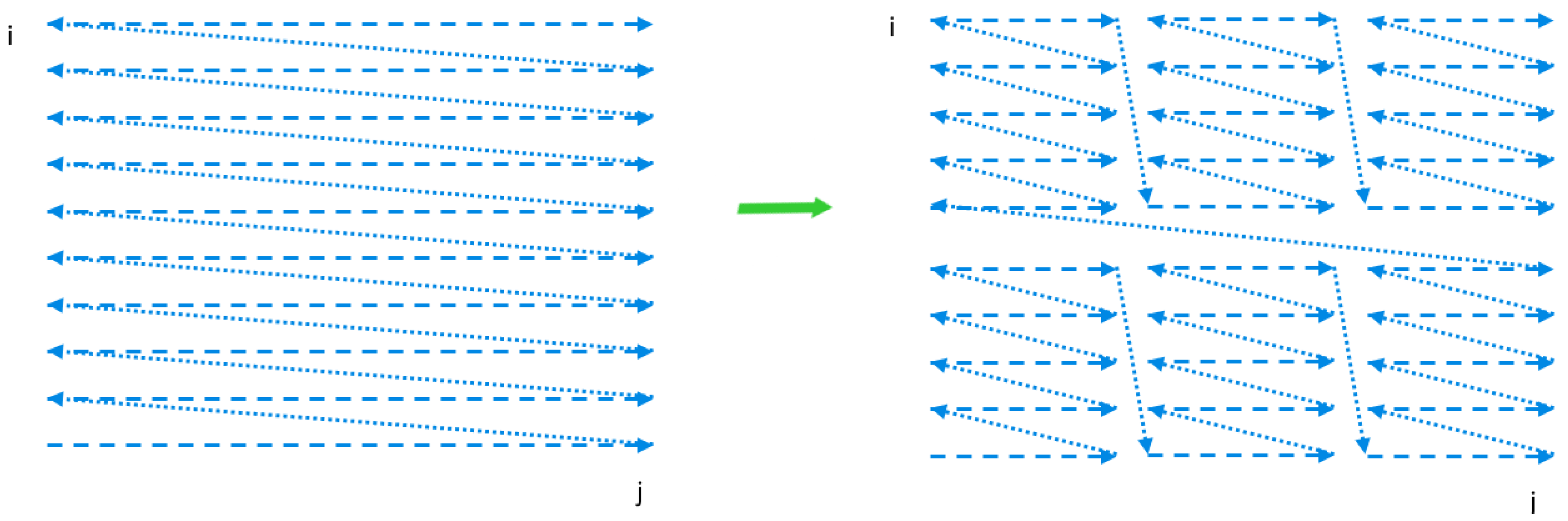
Next, we use the concept of a loop nest statement instance schedule, which specifies the order in which those instances are executed in target code. To improve the features of the dependences of the code presented in Listing 1, we suggest applying to the loop nest statements a schedule formed according to the data flow concept DFC): first, the readiness time for each operand of each statement should be defined, for example, if $t_1^i,t_2^i,\dots ,t_k^i$ are k discrete times of the readiness of k operands of statement i, then the schedule of statement i is defined as follows: $t_i=max(t_1^i,t_2^i,\dots ,t_k^i)+1$. On the right of that formula, the first term defines the maximal time among all operand readiness times of statement i, and “+1” means that statement i can be executed at the next discrete time after all its operands are ready (already calculated).

DFC schedules should be defined and applied to all the statements of the source loop nest to generate a transformed serial loop.

Analyzing the operands $c\left[i\right][k-1]$ and $c[k+1][j-1]$ of statement $S0$ in Listing 1 as well as the bounds of loops i and j, we may conclude that their readiness times are $k-i-1$ and $j-k-2$, respectively. We also take into account that element $c\left[i\right]\left[j\right]$ can be updated many times for different values of k, and the final value of $c\left[i\right]\left[j\right]$ is formed in time $j-i-1$. Thus, according to DFC, statement $S0$ is to be executed at time $t=max(k-i-1,j-k-2)+1$ for variables i and j satisfying the constraint $t<=j-i-1$. The last constraint means that element $c\left[i\right]\left[j\right]$ formed with statement $S0$ can be updated many times at time t, satisfying the condition $t<=j-i-1$. Thus, taking into account the global schedule of statement $S0$ represented with relation $M0$, we obtain the following DFC schedule, $SCHED\left(S0\right)$.

$$SCHED\left(S0\right):=N\to \{S_0(i,j,k)\to t=max(k-i-1,j-k-2)+1,-i,j,0,k)\mid t\le j-i-1\}.$$

Analyzing statement $S1$, we may conclude that it should be executed when for given i and j, loop k is terminated, that is, the calculation of the value of element $c\left[i\right]\left[j\right]$ is terminated, that is, at time $j-i-1$. Thus, we obtained the following schedule for statement $S1$ taking into account the global schedule for $S1$ presented with relation $M1$ above.

$$SCHED\left(S1\right):=N\to \{S_0(i,j,k)\to (t=max(k-i-1,j-k-2)+1,-i,j,1,0)\mid t=j-i-1\}.$$

The constraint $t=j-i-1$ means that statement $S1$ can be updated only when loop k is terminated. Constant 1 in the third position of the tuple $(t=max(k-i-1,j-k-2)+1,-i,j,1,0)$ guarantees that statement $S1$ should be executed after terminating all the iterations of loop k.

Applying schedules $SCHED\left(S0\right)$ and $SCHED\left(S1\right)$ to statements $S0$ and $S1$, by means of the codegen iscc operator, we obtain the transformed code presented in Listing 4.

Listing 4. Transformed C code implementing the counting algorithm

1 for (int c0 = 1; c0 < N − 1; c0 += 1)   2  for (int c1 = −N + c0 + 1; c1 < 0; c1 += 1)   3   for (int c2 = c0 − c1 + 1; c2 <= min(N, 2 ∗ c0 − c1 + 1); c2 += 1) {   4    if (2 ∗ c0 >= c1 + c2)   5    {   6     c[−c1][c2] += paired(−c0 + c2 − 1, c2) ? c[−c1][−c0 + c2 − 1 − 1] + c[−c0 + c2 − 1 + 1][c2 − 1] : 0;   7    }   8    c[−c1][c2] += paired(c0 − c1, c2) ? c[−c1][c0 − c1 − 1] + c[c0 − c1 + 1][c2 − 1] : 0;   9    if (c1 + c2 == c0 + 1) 10    { 11     c[−c1][c0 − c1 + 1] = c[−c1][c0 − c1 + 1] + c[−c1][c0 − c1 + 1 − 1]; 12    } 13   }

That code respects all dependences available in the code in Listing 1 due to the following reason. In the code in Listing 1, we distinguish two types of dependences: standard ones and reductions. If the loop nest statement uses an associative and commutative operation such as addition, we recognize the dependence between two references of this statement as a reduction dependence [19]. For example, in the code in Listing 1, statement $S0$

$$c\left[i\right]\left[j\right]+=paired(k,j)?c\left[i\right][k-1]+c[k+1][j-1]:0;//S0$$

causes reduction dependences regarding to reads and writes of element $c\left[i\right]\left[j\right]$.

We may allow them to be reordered provided that a new order is serial, that is, reduction dependences do not impose an ordering constraint; in the code in Listing 4, reduction dependences are respected due to the serial execution of loop nest statement instances.

Standard dependences available in the code in Listing 1 are respected via implementing the DFC concept.

To prove the validity of the applied schedules to generate the code in Listing 4 in a formal way, we use the schedule validation technique presented in the Ref. [20].

Given relation F representing all the dependences to be respected, schedule S is valid if the following inequality is true:

$$\Delta (S\circ F\circ S^{-1})⪰0,$$

where $\Delta$ is the operator that maps a relation to the differences between image and domain elements.

The result of the composition $R=(S\circ F\circ S^{-1})$ is a relation where the input (left) and output (right) tuples represent dependence sources and destinations, respectively, in the transformed iteration space. A schedule is valid (respects all the dependences available in an original loop nest) if the vector whose elements are the differences between the image and domain elements of relation R is lexicographically non-negative ($⪰0$). In such a case, each standard dependence in the original loop nest is respected in the transformed loop nest.

To apply the schedule validity technique above, we extract dependence relations F by means of PET. Then we eliminate from F all reduction dependences, taking into account the fact that such dependences cause only statement $S0$. We present reduction dependences by means of the following relation:

$$\{S_0(i,j,k)\to S_0(i,j,k^{\prime })\mid k^{\prime }>k\}.$$

Next, applying the iscc calculator, we obtain a relation, R, as the result of the composition $(S\circ F\circ S^{-1})$, where S is the union of schedules $SCHED\left(S0\right)$ and $SCHED\left(S1\right)$ defined above to generate the target code.

To check whether each vector represented with set $C=\Delta (S\circ F\circ S^{-1})$ is lexicographically non-negative, we form the following set that represents all lexicographically negative vectors in the unbounded 5D space.

$LD5:=N\to \left\{\right(t,i0,i1,i2,i3)\mid t<0\}\cup N\to \left\{\right(0,i0,i1,i2,i3)\mid i0<0\}\cup N\to \left\{\right(0,0,i1,i2,i3)\mid i1<0\}\cup N\to \left\{\right(0,0,0,i2,i3)\mid i2<0\}\cup N\to \left\{\right(0,0,0,0,i3)\mid i3\le 0\}.$

Then, we calculate the intersection of sets C and $LD5$. That intersection is the empty set, that means that all vectors of C are lexicographically non-negative. This proves the validity of schedules $SCHED\left(S0\right)$ and $SCHED\left(S1\right)$.

For the code presented in Listing 4, by means of PET and the iscc calculator, we obtained the following distance vectors.

• $D1:=\left\{\right(i0,i1,1,i3)\mid i0\ge 2\wedge -1\le i3\le 1\wedge ((i1\ge 2+i0\wedge i3\ge 0)\vee (i1>0\wedge i3\le 0)\left)\right\}$,
• $D2:=\left\{\right(2,0,i2,-1)\mid i2\ge 2\}$,
• $D3:=\left\{\right(i0,0,i2,i3)\mid i3\le 2\wedge ((i0\ge 3\wedge i2\ge 3+i0\wedge -2\le i3\le 0)\vee (i0\ge 2\wedge i2\ge 2\wedge 0\le i3\le 1)\vee (0\le i2\le 1\wedge i2\le i0\wedge i3\ge i2\wedge i3>-i0)\left)\right\}$,
• $D4:=\left\{\right(2,i1,1,-2)\mid i1>0\}$,
• $D5:=\left\{\right(1,0,1,0\left)\right\}$,
• $D6:=\left\{\right(i0,0,0,-1)\mid i0>0\}$.

To simplify extracting affine transformations, we approximate the distance vectors above with a single distance vector, which represents each distance vector presented above. $D:=\left\{\right(i0,i1,1,i3)\mid i0\ge 0\wedge i1\ge 0\wedge i2\ge 0\wedge -2\le i3\le 2$. The time partitions constraint formed on the basis of the vector above is the following.

$$x_0\ast i0+x_1\ast i1+x_2\ast i2+x_3\ast i3\ge 0,constraints$$

(3)

where $x_0,x_1,x_2,x_3$ are unknowns, and $constraints$ represent the constraints of set D above.

Taking into account that unknown $x3$ should be 0 because variable $i3$ is not any loop iterator, it represents global schedule constants and it should not be transformed. There exist three linearly independent solutions to constraint (3), for example, ${(1,0,0,0)}^T,{(0,1,0,0)}^T$ and ${(0,0,1,0)}^T$.

Applying the DAPT optimizing compiler [21], which automatically extracts and applies the affine transformations to the code in Listing 4 to tile and parallelize that code by means of the wave-front technique [22], we obtain the following target 3D tiled parallel code (Listing 5) with tiles of size 16 × 32 × 40. By means of experiments, this size was defined by us as the optimal one regarding tiled code performance.

In that code, the first three loops enumerate tiles, while the remaining three loops scan statement instances within each tile. The OpenMP [23] directive $\#pragmaompparallelfor$ makes the loop for (int h0=...) parallel.

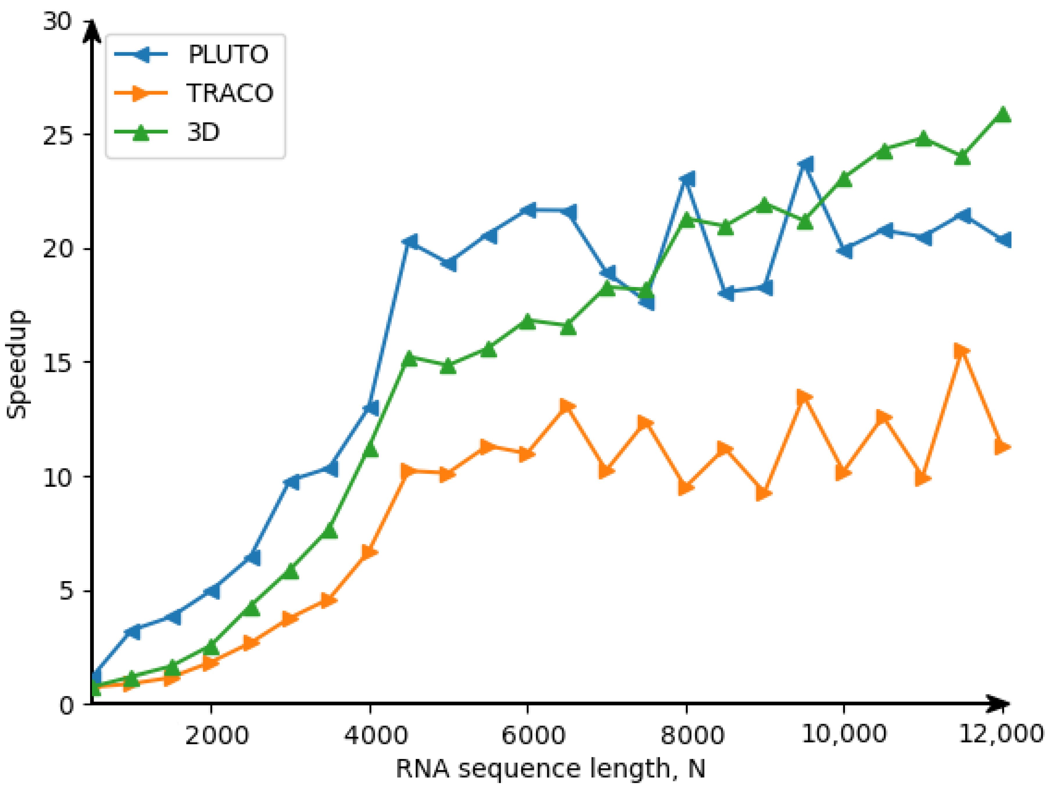
The Ref. [24] illustrates the advantage of 3D tiled codes in comparison with 2D tiled ones which implement RNA Nussinov’s algorithm [25]. However, there are the following differences between the approaches used for code generation for the Nussinov problem [24] and for the counting problem considered in the current paper. The code for the Nussinov problem is derived on the idea of a calculation model based on systolic arrays (first figure in the Nussinov paper), while code for the counting problem is based on the data flow concept (DFC). The approach presented in the current paper uses the validity technique of the applied schedules to generate target code, while the approach presented in the Nussinov paper does not envisage any formal validation of applied schedules.

Listing 5. 3D tiled parallel code

1 for (int w0 = floord(−N + 34, 160) − 1; w0 < floord(7 ∗ N − 10, 80); w0 += 1) { 2  #pragma omp parallel for 3  for (int h0 = max(max(0, w0 − (N + 40) / 40 + 2), w0 + floord(−4 ∗ w0 − 3, 9) + 1); h0 <= min((N − 2) / 16, w0 + floord(N − 80 ∗ w0 + 46, 240) + 1); h0 += 1) { 4   for (int h1 = max(max(max(5 ∗ w0 − 9 ∗ h0 − 3, −((N + 29) / 32)), w0 − h0 − (N + 40) / 40 + 1), −((N − 16 ∗ h0 + 30) / 32)); h1 <= min(−1, 5 ∗ w0 − 7 ∗ h0 + 8); h1 += 1) { 5    for (int i0 = max(max(1, 16 ∗ h0), 20 ∗ w0 − 20 ∗ h0 − 4 ∗ h1); i0 <= min(min(16 ∗ h0 + 15, N + 32 ∗ h1 + 30), 40 ∗ w0 − 40 ∗ h0 − 8 ∗ h1 + 69); i0 += 1) { 6     for (int i1 = max(max(32 ∗ h1, −40 ∗ w0 + 40 ∗ h0 + 40 ∗ h1 + i0 − 38), −N + i0 + 1); i1 <= min(32 ∗ h1 + 31, −40 ∗ w0 + 40 ∗ h0 + 40 ∗ h1 + 2 ∗ i0 + 1); i1 += 1) { 7      for (int i2 = max(40 ∗ w0 − 40 ∗ h0 − 40 ∗ h1, i0 − i1 + 1); i2 <= min(min(N, 40 ∗ w0 − 40 ∗ h0 − 40 ∗ h1 + 39), 2 ∗ i0 − i1 + 1); i2 += 1) { 8       { 9        if (2 ∗ i0 >= i1 + i2) { 10         c[−i1][i2] += (paired((−i0 + i2 − 1), (i2)) ? (c[−i1][−i0 + i2 − 2] + c[−i0 + i2][i2 − 1]) : 0); 11        } 12        c[−i1][i2] += (paired((i0 − i1), (i2)) ? (c[−i1][i0 − i1 − 1] + c[i0 − i1 + 1][i2 − 1]) : 0); 13        if (i1 + i2 == i0 + 1) { 14         c[−i1][i0 − i1 + 1] = (c[−i1][i0 − i1 + 1] + c[−i1][i0 − i1]); 15        } 16       } 17      } 18     } 19    } 20   } 21  } 22 }

2.3. Related Codes

To our best knowledge, there is no manual implementation (as parallel tiled code) of the counting algorithm. To generate such a code, we chose two optimizing compilers, PLUTO and TRACO. They are open source codes and allow for automatic code optimization (tiling and parallelization). We did not consider other optimizing compilers because they do not satisfy one or more of the following demands: the compiler must be a source-to-source translator, it should be able to tile and parallelize source code, be based on polyhedral techniques, be currently maintained and have no building problems, and be well-documented. Applying PLUTO to counting source code allows us to generate only 2D tiled parallel code while applying TRACO results in the generation of codes with irregular tiles.

The usefulness of generated tiled parallel code presented in this paper is the following. In relation to the 2D tiled PLUTO code, the generated code by means of the presented approach is 3D. This allows us to increase code locality and, as a consequence, improve target code performance. With regard to the PLUTO code, 3D tiled code enumerates regular bounded tiles that allows for improving code locality in comparison with the PLUTO code, and this results in improving code performance. The tile regularity of 3D tiled code also provides better code locality in comparison with the TRACO code because a tile size is limited and there is a possibility to choose a tile size such that all the data associated with a single tile can be held in cache.

Listing 6. PLUTO [13] code implementing the counting algorithm

1 if (N >= 3) 2 { 3  for (t1 = 3; t1 <= N; t1++) 4  { 5   lbp = 0; 6   ubp = floord(t1 − 2, 32); 7 #pragma omp parallel for private(lbv, ubv, t3, t4, t5) 8   for (t2 = lbp; t2 <= ubp; t2++) 9   { 10    for (t3 = t2; t3 <= floord(t1, 32); t3++) 11    { 12     if ((t1 >= 32 ∗ t3 + 1) && (t1 <= 32 ∗ t3 + 31)) 13     { 14      for (t4 = max(1, 32 ∗ t2); t4 <= min(t1 − 2, 32 ∗ t2 + 31); t4++) 15      { 16       for (t5 = max(32 ∗ t3, t4); t5 <= t1 − 1; t5++) 17       { 18        c[t4][t1] += paired(t5, t1) ? c[t4][t5 − 1] + c[t5 + 1][t1 − 1] : 0; 19       } 20       c[t4][t1] = c[t4][t1] + c[t4][t1 − 1]; 21      } 22     } 23     if (t1 >= 32 ∗ t3 + 32) 24     { 25      for (t4 = max(1, 32 ∗ t2); t4 <= min(t1 − 2, 32 ∗ t2 + 31); t4++) 26      { 27       for (t5 = max(32 ∗ t3, t4); t5 <= 32 ∗ t3 + 31; t5++) 28       { 29        c[t4][t1] += paired(t5, t1) ? c[t4][t5 − 1] + c[t5 + 1][t1 − 1] : 0; 30       } 31      } 32     } 33     if (t1 == 32 ∗ t3) 34     { 35      for (t4 = max(1, 32 ∗ t2); t4 <= min(t1 − 2, 32 ∗ t2 + 31); t4++) 36      { 37       if (t1 % 32 == 0) 38       { 39        c[t4][t1] = c[t4][t1] + c[t4][t1 − 1]; 40       } 41      } 42     } 43    } 44   } 45  } 46 }

The codes used for comparison are presented below. These codes were obtained from the code in Listing 1. The code in Listing 6 is generated by the PLUTO parallel compiler [13] and the code in Listing 7 is generated by TRACO [14].

The code in Listing 6 enumerates 2D tiles of size 32 × 32, which was established as the optimal one by us via experiments. PLUTO implements the affine transformation framework, and as we demonstrate in Section 2.2, there exist only two linearly independent solutions for the time partition constraints formed for the code in Listing 1. Thus, the maximal dimension of the tiles in the code in Listing 6 is 2D.

Traco generates 3D tiles of size $8\times 127\times 16$ (defined by us as the optimal one by means of experiments), but tiles are irregular, some of them are unbounded, hampering thread load balance and reducing code locality because not all the data associated with a single unbounded tile can be held in the cache.

Listing 7. TRACO [14] code implementing the counting algorithm

1 for (c1 = 0; c1 < N + floord(N − 3, 128) − 2; c1 += 1) 2 #pragma omp parallel for 3  for (c3 = max(0, −N + c1 + 3); c3 <= c1 / 129; c3 += 1) 4   for (c4 = 0; c4 <= 1; c4 += 1) 5   { 6    if (c4 == 1) 7    { 8     for (c9 = N − c1 + 129 ∗ c3; c9 <= min(N, N − c1 + 129 ∗ c3 + 127); c9 += 1) 9      for (c10 = max(0, −c1 + 64 ∗ c3 − c9 + (N + c1 + c3 + c9 + 1) / 2 + 1); c10 <= 1; c10 += 1) 10      { 11       if (c10 == 1) 12       { 13        c[(N − c1 + c3 − 2)][c9] = c[(N − c1 + c3 − 2)][c9] + c[(N − c1 + c3 − 2)][c9 − 1]; 14       } 15       else 16       { 17        for (c11 = N − c1 + 129 ∗ c3 + 1; c11 < c9; c11 += 1) 18         c[(N − c1 + c3 − 2)][c9] += paired(c11, c9) ? c[(N − c1 + c3 − 2)][c11 − 1] + c[c11 + 1][c9 − 1] : 0; 19       } 20      } 21     } 22     else 23     { 24      for (c5 = 0; c5 <= 8 ∗ c3; c5 += 1) 25       for (c9 = N − c1 + 129 ∗ c3; c9 <= min(N, N − c1 + 129 ∗ c3 + 127); c9 += 1) 26        for (c11 = N − c1 + c3 + 16 ∗ c5 − 2; c11 <= min(min(N − c1 + 129 ∗ c3, N − c1 + c3 + 16 ∗ c5 + 13), c9 − 1); c11 += 1) 27         c[(N − c1 + c3 − 2)][c9] += paired(c11, c9) + c[(N − c1 + c3 − 2)][c11 − 1] + c[c11 + 1][c9 − 1] + 0; 28     } 29 }

3. Results

First we show impact of the number of threads on performace in Figure 2 and Figure 3. To carry out the experiments, we used two machines: (i) a processor Intel(R) Xeon(R) Gold 6326 (2.90GHz, 2 physical units, 32 cores, 64 threads, 24 MB Cache) (results obtained on that machine are presented in Figure 4 and Figure 5) and (ii) a processor Intel(R) i7-11700KF (3.6GHz, 8 cores, 16 threads, 16MB Cache), where results achieved on that machine are depicted in Figure 6 and Figure 7. All examined codes were compiled by means of the gcc 11.3 compiler with the –O3 flag of optimization. The reason for using this option was to generate optimal serial and parallel executable code. Codes without this option run much longer for both sequential and parallel code.

Experiments were carried out for 24 RNA randomly generated sequence lengths of the problem defined with parameter N from 500 to 12,000. The results presented in the Refs. [26,27] show that cache-efficient code performance does not change based on the strings themselves, but it depends on the size of a string. We also performed a study with a variable number of threads, with sequence length 12,000 on Intel Xeon and sequence length 10,000 on Intel i7. We used a range from 1 to 32 threads with step 1 for both machines. Results are shown in Figure 2 and Figure 3. We compared the performance of the 3D tiled code generated with the presented approach with that of the following codes:

1

Listing 6—PLUTO parallel tiled code (based on affine transformations) (PLUTO in charts) [13].

2

Listing 7—Tiled code based on the correction technique (TRACO in charts) [14].

3

Listing 1—Original code of counting algorithm (ORIGINAL in charts) [7,8].

All source codes used for carrying out experiments as well as a program allowing us to run each parallel program for a random or real RNA strand can be found in the Data Availability section.

3.1. Impact of the Number of Threads on Code Performance

3.1.1. Intel Xeon

Figure 2 shows the speedup of the three examined parallel codes—the ratio of the serial code execution time to that of the parallel one. The 3D code speedup demonstrates nearly linear speedup. From this chart, it can be assumed that the 3D code is well-scalable, that is, it is possible to increase code parallelism further when increasing the number of threads. The 3D code can be run on a machine with a large number of threads without any code modification.

3.1.2. Intel i7

Figure 3 shows the speedup of the same parallel codes on a i7 processor. The important part of this chart is between 12 and 16 threads (16 threads is the maximum for this unit). From this chart, it can be assumed that the 3D code works very well at the maximum level of threads, and it is also possible to increase code parallelism further when increasing the number of cores and threads.

3.2. Impact of the Problem Size on Code Performance

3.2.1. Intel Xeon

For the results depicted in Figure 4 and Figure 5, one can see a clear advantage of the 3D code for larger problem sizes. For smaller problem sizes, taking into account how the PLUTO code is simpler than 3D code (it comprises 5 loops while 3D code includes 6 loops), that is, PLUTO executes less iterations than 3D code does, it demonstrates better performance than that of the 3D code, while for larger problem sizes, better code locality of 3D code in comparison with that of PLUTO one outweighs the benefits of PLUTO code simplicity.

3.2.2. Intel i7

The code in Figure 6 shows that with a larger problem size, it is possible to calculate faster for the 3D code. In addition to that, the 3D code is characterized by much greater stability of performance (no spikes in speedup for the both processors tested).

In addition to that, Figure 7 shows that for the 3D code, it is possible to utilize the available threads fully. However, with more threads than the number of threads available on the processor, the operation of this code is not the fastest one.

4. Discussion

The approach presented in this paper allows for parallel tiled code generation for the counting algorithm. Target code demonstrates a significant increase in code performance, largely over original sequential code. For larger problem sizes, it outperforms related parallel tiled codes and exposes better scalability. The experimental results carried out by us show that the 3D parallel tiled code, implementing the counting algorithm, utilises computational capabilities of modern processor cores very well. The advantages of the obtained 3D code are more obvious for a large problem size. We plan to apply the presented approach to other bioinformatics codes whose dependence patterns are similar to those available in the code implementing the counting algorithm. This allows for increasing the tile dimension as a consequence of increasing the performance and scalability of target codes. We also intend to fully automate the process of target code generation and implement it in an optimizing compiler.

References

1. Nawaz, Z.; Nadeem, M.; van Someren, H.; Bertels, K. A parallel FPGA design of the Smith-Waterman traceback. In Proceedings of the 2010 International Conference on Field-Programmable Technology, Beijing, China, 8–10 December 2010; Volume 18, pp. 454–459. [Google Scholar]
2. Manavski, S.A.; Valle, G. CUDA compatible GPU cards as efficient hardware accelerators for Smith-Waterman sequence alignment. BMC Bioinform. 2008, 9, S10. [Google Scholar] [CrossRef] [PubMed]
3. Gruzewski, M.; Palkowski, M. RNA Folding Codes Optimization Using the Intel SDK for OpenCL. In Proceedings of the Artificial Intelligence and Soft Computing: 20th International Conference, ICAISC 2021, Virtual Event, 21–23 June 2021; Springer: Cham, Switzerland, 2021; Volume 12855. [Google Scholar]
4. Gruzewski, M.; Palkowski, M. Implementation of Nussinov’s RNA Folding Using the Kokkos Library. In Progress in Image Processing, Pattern Recognition and Communication Systems, Proceedings of the Conference (CORES, IP&C, ACS), Virtual Event, 28–30 June 2021; Springer: Cham, Switzerland, 2022; Volume 255, pp. 15–30. [Google Scholar]
5. Palkowski, M.; Bielecki, W. Tiling Nussinov’s RNA folding loop nest with a space-time approach. BMC Bioinform. 2019, 20, 208. [Google Scholar] [CrossRef]
6. Smith, T.F.; Waterman, M.S. Identification of common molecular subsequences. J. Mol. Biol. 1981, 147, 195–197. [Google Scholar] [CrossRef] [PubMed]
7. Raden, M.; Mohamed, M.M.; Ali Syed, M.; Backofen, R. Interactive implementations of thermodynamics-based RNA structure and RNA-RNA interaction prediction approaches for example-driven teaching. PLoS Comput. Biol. 2018, 14, e1006341. [Google Scholar] [CrossRef]
8. Raden, M.; Ali, S.M.; Alkhnbashi, O.S.; Busch, A.; Costa, F.; Davis, J.A.; Eggenhofer, F.; Gelhausen, R.; Georg, J.; Heyne, S.; et al. Freiburg RNA tools: A central online resource for RNA-focused research and teaching. Nucleic Acids Res. 2018, 46, W25–W29. [Google Scholar] [CrossRef] [PubMed]
9. Bondhugula, U.; Baskaran, M.; Krishnamoorthy, S.; Ramanujam, J.; Rountev, A.; Sadayappan, P. Automatic Transformations for Communication-Minimized Parallelization and Locality Optimization in the Polyhedral Model. In Compiler Construction, Proceedings of the 17th International Conference, CC 2008, Held as Part of the Joint European Conferences on Theory and Practice of Software, ETAPS 2008, Budapest, Hungary, 29 March–6 April 2008; Springer: Berlin/Heidelberg, Germany, 2008; pp. 132–146. [Google Scholar]
10. Lim, A.; Cheong, G.L.; Lam, M.S. An Affine Partitioning Algorithm to Maximize Parallelism and Minimize Communication. In Proceedings of the 13th International Conference on Supercomputing, Rhodes, Greece, 20–25 June 1999; pp. 228–237. [Google Scholar]
11. Wolf, M.E.; Lam, M.S. A data locality optimizing algorithm. In Proceedings of the ACM SIGPLAN 1991 Conference on Programming Language Design and Implementation, Toronto, ON, Canada, 26–28 June 1991; pp. 30–44. [Google Scholar]
12. Xue, J. Loop Tiling for Parallelism; Springer: Berlin/Heidelberg, Germany, 2000; Volume 575. [Google Scholar]
13. Bondhugula, U.; Hartono, A.; Ramanujam, J.; Sadayappan, P. Pluto: A practical and fully automatic polyhedral program optimization system. In Proceedings of the ACM SIGPLAN 2008 Conference on Programming Language Design and Implementation (PLDI 08), Tucson, AZ, USA, 7–13 June 2008; pp. 101–113. [Google Scholar]
14. Palkowski, M.; Bielecki, W. TRACO parallelizing compiler. In Soft Computing in Computer and Information Science; Springer: Cham, Switzerland, 2015; pp. 409–421. [Google Scholar]
15. Mullapudi, R.T.; Bondhugula, U. Tiling for dynamic scheduling. In Proceedings of the 4th International Workshop on Polyhedral Compilation Techniques, Vienna, Austria, 20 January 2014; Volume 20. [Google Scholar]
16. Palkowski, M.; Bielecki, W. Tuning iteration space slicing based tiled multi-core code implementing Nussinov’s RNA folding. BMC Bioinform. 2018, 19, 12. [Google Scholar] [CrossRef] [PubMed]
17. Verdoolaege, S. Counting affine calculator and applications. In Proceedings of the First International Workshop on Polyhedral Compilation Techniques (IMPACT’11), Chamonix, France, 3 April 2011. [Google Scholar]
18. Verdoolaege, S.; Grosser, T. Polyhedral extraction tool. In Proceedings of the First Second International Workshop on Polyhedral Compilation Techniques (IMPACT’12), Paris, France, 23 January 2012. [Google Scholar]
19. Pugh, W.; Wonnacott, D. Static analysis of upper and lower bounds on dependences and parallelism. ACM Trans. Program. Lang. Syst. (TOPLAS) 1994, 16, 1248–1278. [Google Scholar] [CrossRef]
20. Verdoolaege, S.; Carlos Juega, J.; Cohen, A.; Ignacio Gomez, J.; Tenllado, C.; Catthoor, F. Polyhedral parallel code generation for CUDA. ACM Trans. Archit. Code Optim. (TACO) 2013, 9, 1–23. [Google Scholar] [CrossRef]
21. Bielecki, W.; Poliwoda, M. Automatic parallel tiled code generation based on dependence approximation. In International Conference on Parallel Computing Technologies; Springer: Berlin/Heidelberg, Germany, 2021; pp. 260–275. [Google Scholar]
22. Kennedy, K.; Allen, J.R. Optimizing Compilers for Modern Architectures: A Dependence-Based Approach; Morgan Kaufmann Publishers Inc.: San Francisco, CA, USA, 2001. [Google Scholar]
23. Van der Pas, R.; Stotzer, E.; Terboven, C. Using OpenMP# The Next Step: Affinity, Accelerators, Tasking, and SIMD; MIT Press: Cambridge, MA, USA, 2017. [Google Scholar]
24. Bielecki, W.; Błaszyński, P.; Pałkowski, M. 3D Tiled Code Generation for Nussinov’s Algorithm. Appl. Sci. 2022, 12, 5898. [Google Scholar] [CrossRef]
25. Nussinov, R.; Pieczenik, G.; Griggs, J.R.; Kleitman, D.J. Algorithms for loop matchings. SIAM J. Appl. Math. 1978, 35, 68–82. [Google Scholar] [CrossRef]
26. Li, J.; Ranka, S.; Sahni, S. Multicore and GPU algorithms for Nussinov RNA folding. BMC Bioinform. 2014, 15, S1. [Google Scholar] [CrossRef]
27. Zhao, C.; Sahni, S. Cache and energy efficient algorithms for Nussinov’s RNA folding. BMC Bioinform. 2017, 18, 15–30. [Google Scholar] [CrossRef] [Green Version]
Figure 1. Loop transformation.
Eng 04 00030 g001
Figure 2. Speedup for different thread numbers. Intel Xeon—sequence length 12,000.
Eng 04 00030 g002
Figure 3. Speedup for different thread numbers. Intel i7—sequence length 10,000.
Eng 04 00030 g003
Figure 4. Speedup for different sequence lengths. Intel Xeon—16 threads.
Eng 04 00030 g004
Figure 5. Speedup for different sequence lengths. Intel Xeon—32 threads.
Eng 04 00030 g005
Figure 6. Speedup for different sequence lengths. Intel i7—16 threads.
Eng 04 00030 g006
Figure 7. Speedup for different sequence lengths. Intel i7—32 threads.
Eng 04 00030 g007
Disclaimer/Publisher’s Note: The statements, opinions and data contained in all publications are solely those of the individual author(s) and contributor(s) and not of MDPI and/or the editor(s). MDPI and/or the editor(s) disclaim responsibility for any injury to people or property resulting from any ideas, methods, instructions or products referred to in the content.