Article

Measuring the Diffusion Coefficient of Paste and Concrete by Using Dental X-ray Equipment

1
Virginia Transportation Research Council (VTRC), Charlottesville, VA 22903, USA
2
School of Civil & Environmental Engineering, Oklahoma State University, 248 Engineering North, Stillwater, OK 74078, USA
3
Brorsen Family Dental Clinic, Stillwater, OK 74075, USA
*
Author to whom correspondence should be addressed.
CivilEng 2023, 4(1), 224-247; https://doi.org/10.3390/civileng4010014
Submission received: 28 December 2022 / Revised: 20 February 2023 / Accepted: 21 February 2023 / Published: 24 February 2023
(This article belongs to the Special Issue Feature Papers in CivilEng)

Abstract

:
The penetration of ions plays an important role in the durability of concrete structures. This study aims to establish the feasibility of using dental X-ray equipment to measure the concentration and penetration of iodide within cementitious systems. This technique is known as checking ion penetration (CHIP). This test uses iodide as a tracer because it has a high electron density, and so it can be observed with X-ray imaging as it penetrates the concrete. Concentration profiles from CHIP are used to calculate the apparent diffusion coefficient (Dac). These results are similar to measurements from bulk chloride ponding tests. The Dac is used to predict the service life or evaluate the quality of an as-built concrete structure or concrete mixture. Because of the wide availability of dental equipment, CHIP shows promise to be used as a method to measure the in-place quality control of the concrete.

1. Introduction

Concrete has been used for over a century as the building material of choice for long service life. The durability of concrete is often threatened by the transport of outside ions that cause deterioration of the concrete or the reinforcing [1]. The most common way to quantify the resistance to outside chemical penetration is by using electrical methods to indirectly investigate the microstructure. The most common electrical tests are the rapid chloride permeability test (ASTM C1202) and the electrical resistivity tests (AASHTO TP95 and ASTM C 1760). These tests have challenges predicting the resistance to outside chemicals when supplementary cementing materials (SCMs), certain chemical admixtures, steel fibers, and some particular aggregates are used in the mixtures, or when the temperature/moisture or amount of carbonation content varies within the mixtures [2,3,4,5,6,7,8,9,10].
The most trusted method to investigate ion ingress into cement-based materials is the bulk diffusion test. This test is completed by placing a salt solution on top of the sample as described in ASTM C 1556 and AASHTO T259, followed by a titration test on powder taken at different depths within the sample [11,12,13,14]. Because the powder from the concrete contains about 75% aggregate and 25% paste by volume, a large amount of powder is needed to be sure that the chlorides in the paste are well characterized. These tests are time-consuming and labor-intensive, and so they are not widely used.
Several studies have used X-ray imaging techniques to simplify the ASTM C 1556 test. Some of these include using X-ray fluorescence (XRF) and X-ray microtomography [15,16,17,18,19,20,21,22,23,24,25,26]. The equipment needed for these measurements is expensive, time-consuming, and needs significant sample preparation. Recently, transmission X-ray microscopy (TXM) using µCT equipment has been used to place iodide in water and observe the change in X-ray absorption. TXM is useful because it is non-destructive, fast, requires minimal sample preparation, and the technique can image at a spatial resolution of 200 nm to 20 μm [27,28,29,30,31,32]. TXM is a non-destructive technique (NDT), and so it allows the sample to continue to be investigated with TXM to study the penetration of ions with time, or the same sample could be used in another experiment such as porosity, X-ray diffraction, or microstructure imaging. The apparent diffusion coefficient from TXM and X-ray fluorescence (µXRF) mapping is within 5% to 13.5% [27]. Others have compared the rate of iodide penetration to the rate of chlorides, and the results indicate that iodide serves as a satisfactory tracer to represent the diffusion and penetration of chloride in a cementitious system. More details are provided in Appendix A.
The goal of this study is to develop a test method that is guided by TXM but uses low-cost and widely available dental X-ray equipment to determine the rate of fluid transport within cement-based materials with less time and cost. This device will be known as checking ion penetration (CHIP). The main components of a dental X-ray unit are the control panel, tube head, position-indicator device (PID), and sensor (or indicator). Like X-rays taken in other applications, dental X-rays use electromagnetic radiation to capture images of the object of interest. The radiation beam generated from the tube head passes through the object, reaches the sensor, and creates 2D images of the object.
Emerging countries are creating massive volumes of concrete infrastructure, and more testing is needed to evaluate the durability of their in-place concrete. Annual world cement production (which can represent concrete production indirectly) is expected to increase considerably from now to 2050. The largest share of this growth will take place in China, India, and other developing countries on the Asian continent [33]. The growth of concrete demand increases the need for a widely available, reliable, fast, and economic test method to evaluate the durability performance of the produced concrete. Since dental equipment is so ubiquitous and CHIP requires very simple sample preparation, this makes CHIP a promising technique for emerging countries to use as a viable quality control method to evaluate the durability of their concrete. Moreover, the performance of different cementitious systems (e.g., types of cement, admixtures, SCMs, latex and polymer additives, etc.) and different construction and repair techniques and practices (e.g., surface finishing and treatment, sealers, concrete pouring, and casting methods, curing methods, etc.) can be evaluated by CHIP in a short time. Therefore, CHIP can be used as a reliable and fast technique to evaluate the long-term performance of a technique or method before implementing it in the field. This performance evaluation capability could be used to help practitioners make informed decisions in choosing a proper material or construction practice for each project to meet the long-term requirements and expectations of that project.

2. Overview of the Experiments

This study is divided into two parts. The first will focus on establishing CHIP, and the second will determine the variability of the method. In the first part, the results of CHIP are compared with TXM. The investigated samples are summarized in Table 1. The concrete samples were cored from ten different bridge decks. Two more miniature cores were taken from one of the bridge decks to complete Part II of the study. Therefore, in total, twelve concrete samples were tested. Next, the variability of CHIP was investigated by looking at a larger number of samples.

3. Methods

3.1. Sample Preparation

3.1.1. Materials

For making the paste samples, ASTM C150 Type I Portland cement [34] was used. The chemical composition of the cement is shown in Table 2. Tap water at room temperature was used during the mixing. No chemical admixtures or secondary cementitious material were used in these samples.

3.1.2. Mixture Proportion and Mixing

Mixture proportions of the paste samples are provided in Table 3. The paste samples investigated had three different water-to-cement (w/cm) ratios of 0.35, 0.40, and 0.45. Different w/cm ratios were chosen to create samples with different fluid transport properties. The components were mixed according to ASTM C305 [35].

3.1.3. Sample Preparation

Paste Samples

Cylindrical micro vials with an inside dimension of 9.5 mm × 46 mm were used as a mold to cast samples, as shown in Figure 1. Vials were partially filled within 5 mm of the top to provide a space for ponding solution on top of the sample. The samples were consolidated by physically rodding with a 1.45 mm wire. The consolidation was considered to be finished when all visible air voids were removed from the samples. Twenty-seven samples were made from each mixture. Then, the plastic lids of the vials were closed. The sealed samples were then transferred into a covered box in a 23 °C moist curing room for 28 d. The moisture room used for curing the samples meets the requirements of ASTM C511 [36].
After curing, a hexagonal nut was attached to the bottom of the samples with epoxy. This nut was matched with the hexagonal socket to load the samples consistently in the X-ray machine at different times. The stage and sample are shown in Figure 2. The hose clamp shown in Figure 1 was used to prevent the movement of the applied solution between the walls of the sample holder and the sample. This ensured that the only penetration into the sample would come from the surface or a one-directional penetration.

Concrete Samples

To investigate CHIP on the concrete samples, twelve 19.05 mm (3/4 in) in diameter cores were taken from ten in-service bridge decks. The prepared samples had different mix designs, w/b ratios, and ages (provided in Appendix B). All sides of the samples except the finished surface were covered with hydrophobic wax. Coating the sides of the sample allows for one-dimensional diffusion from the top. Next, a nut was glued at the bottom of each sample, as shown in Figure 3.

3.2. Diffusion Test

Diffusion is the movement of a substance from an area of high concentration to an area of low concentration. The diffusion test uses 0.6 mol/L potassium iodide (KI) salt solution on top of each sample. The concentration was chosen to obtain satisfactory contrast between the tracer and the sample [27]. Since X-ray imaging can detect materials with high electron density, then the iodide from the KI salt can be imaged as it penetrates the concrete. Fortunately, iodide and chloride ions are similar in size (iodide radius is 206 pm versus a chloride radius of 167 pm). Additionally, previous testing has shown that iodide gives diffusion coefficients 24% higher than chloride [27]. This means that iodide penetration can provide important insights into the ability of cementitious materials to resist ion penetration.
Before starting the test, samples were scanned with both CHIP and TXM to obtain the initial images of the original samples called reference radiographs. To start the diffusion test, 150 mg of the solution was placed on the surface of the paste samples for 14 d. This solution was placed 2 mm above the surface of the paste sample. For the concrete samples, the solution filled the space between the sample and cell walls to reach 2 mm above the sample surface. The KI solution was refreshed every five days to ensure the concentration is constant. During the experiment, the lids of all vials were sealed to prevent evaporation and change in the solution concentration. All samples were kept at room temperature (23 °C) during the experiment. After 14 d of ponding, the same samples were scanned with both CHIP and TXM from the same orientation imaged in reference radiographs to capture subsequent radiographs.
When a solution with high electron density penetrates a sample, the penetrated depths in the subsequent radiographs look different in comparison to the reference radiograph. By comparing the subsequent radiograph of each sample with its reference radiograph, quantitative concentration profiles and penetration depths of the solution can be found. From this concentration profile then the apparent diffusion coefficient and surface concentration can be obtained. These are engineering parameters that combine the impacts of fluid transport mechanisms of diffusion, absorption, convection, and chemical binding in one term. This work compares the results from CHIP and TXM by investigating the measured surface concentration and apparent diffusion coefficient on the same samples in both techniques. This provides a quantitative way to compare the two methods.

3.3. X-ray Imaging Techniques

3.3.1. TXM Method

A laboratory Skyscan 1172 µCT scanner was used. Each sample was loaded on a fixed stage between the X-ray source and the detector. When X-rays are used to investigate the sample, some X-rays are absorbed, and others pass the sample to reach the detector. The detector produces grayscale images called radiographs based on the received X-rays. The schematic view of the mechanism of imaging in this method is shown in Figure 4. Radiographs were grayscale images in which each pixel has a gray value between “0” and “255”. The gray values change by density, thickness, chemistry, or a combination of these. Denser or thicker materials absorb more X-rays and are therefore darker in the TXM radiographs. Air absorbs fewer X-rays and has been commonly displayed as light gray in the background of each radiograph. As the KI solution penetrates the sample, the penetrated depths are subjected to gray value change such that the affected regions become darker, and therefore gray values decrease compared to the reference radiograph.
Since each radiograph should be compared with its reference radiograph, it is necessary to obtain radiographs from identical orientations at each interval of scanning. This identical orientation is obtained by using the stage shown in Figure 2. A consistent orientation is critical when concrete samples are investigated because of the inclusion of the larger aggregates.

3.3.2. CHIP Method

This method was very similar to the TXM. The only differences were the X-ray source and X-ray settings. An overview of this method is shown in Figure 5. Like TXM, captured radiographs are grayscale images in which each pixel has a value between “0” and “255”. Like TXM, to investigate the gray value change in each sample over time, it is necessary to take images at a constant orientation at each measurement. The same sample test setup as shown in Figure 2 was used with CHIP to obtain consistent orientations for each image. One thing to note is that the CHIP measurement only takes 20 s compared to the 60 s for the TXM. This could be helpful when running a large number of samples.

3.4. Data Collection in Both CHIP and TXM Methods

All samples were scanned before applying the solution with both TXM and CHIP to measure the initial gray values for each sample. This image was called a reference radiograph. The elevation used for each sample was recorded to use the same height for taking consistent images at the next imaging time.
To compare the results of CHIP with TXM, the same side of each sample scanned in TXM was scanned in CHIP. As the preliminary results shown in Figure 6 indicate, the diffusion coefficient changes by 8.9% from 14 d of ponding to 28 d of ponding. Therefore, the apparent diffusion coefficient (Dac) reaches an almost constant value after 14 d of ponding. For this reason, the measurements were made after 14 d of ponding with the tracer solution to evaluate the long-term performance of a cementitious system. By assuming that the concrete is uncracked, the Dac obtained after 14 d of ponding can be a good representative of long-term durability performance. The reason that the concrete was assumed to remain uncracked is that by occurring the first crack on the concrete, none of the evaluations of durability characteristics (e.g., porosity, permeability, etc.) are valid, and they change as the concrete cracks more. More details on the data analysis and calculation of Dac are provided in Section 3.5. After applying the 0.6 mol/L KI solution on top of the sample for 14 d, the subsequent radiograph was taken. Before taking the subsequent radiograph of paste samples, the solution in the vial was poured off, the remaining solution was removed by a paper towel, and then the hose clamp was removed. Before taking the second radiograph of concrete samples, samples were pulled out from the solution and then dried off with a paper towel. All the settings used in the TXM and CHIP techniques are summarized in Table 4.

3.5. Data Analysis of Both Imaging Techniques

To be able to compare the images from the two methods, the CHIP images had to be transformed to match the gray value range of the TXM method. To do this a software code [37] was prepared to import each image, process the image, and write the output image in BMP format. More details are explained in Appendix C.
To analyze the radiographs, a software programming code [37] with minimal user intervention was prepared to align the subsequent images taken after 14 d of ponding with the reference image for each sample. Alignment of the radiographs means applying local displacements (i.e., shift and rotation) to the subsequent radiograph of one individual sample in a way to have it projected on the reference radiograph. Then, to obtain the average of gray values at each depth for each sample, the central region of each radiograph with a width of 0.88 mm (approximately 100 pixels in TXM radiographs and 60 pixels in CHIP radiographs) as shown in Figure 7a was used in the analysis. This was done to eliminate edge effects called cupping artifacts [38]. Each line shows the location where the gray value was measured over the depth of the sample. The final gray value profile was an average of all gray value profiles obtained from the considered 100 or 60 lines, as shown in Figure 7b. One limitation of this method is that the measurement will focus on the center of the sample. This means that if the sample is not homogeneous then the results will be different for different angles. This has been discussed in more detail in Section 4.2, and further refinements to the method are being made for future publications.
The natural log of the average gray value profile for each radiograph was subtracted from the natural log of the average gray value profile of the reference radiograph to find the attenuation (Δμ). Equation (1) shows the attenuation (Δµ) was calculated according to the Beer–Lambert law for different depths [39,40].
(Δµ)x = ln(Iref)x − ln(It)x
where (Iref)x is the transmitted X-ray intensity (gray value) at each depth (x) in the radiograph captured before applying the tracer, and (It)x is the transmitted X-ray intensity at the same depth after the sample has been ponded with iodide. To convert the calculated attenuations to concentration, calibration curves were applied. More detail on the calibration curves is provided in Appendix D.
Next, the concentration profiles were fitted by Fick’s second law of diffusion, as expressed in Equation (2). By fitting a curve on each concentration profile, the apparent diffusion coefficient (Dac) and surface concentration (Cs) can be found for each sample. The Dac obtained combines the impact of fluid transport mechanisms of diffusion, absorption, convection, and chemical binding in one term.
C x , t = C s 1 erf x 2 D ac t   C x , 0 = 0   x > 0 ,   C 0 , t = C s   t 0
where x is the distance from the sample surface, t denotes time, Dac is the apparent diffusion coefficient, Cs is surface iodide concentration, C(x,t) represents iodide concentration at the depth of x from the surface after time t, and the erf is the error function.

3.6. Analysis of Variance (ANOVA)

For the paste samples, three different w/cm ratios of 0.35, 0.40, and 0.45 were made. For each w/cm, 27 paste samples were prepared, as shown in Table 1. An analysis of variance (ANOVA) was completed to determine if the experiment results for the different w/cm ratios were statistically different. The w/cm ratio is considered an independent variable with three levels of 0.35, 0.40, and 0.45, and 27 replicates for each level of w/cm. The Dac is considered the dependent variable because it changes with a change in w/cm. To run the ANOVA, the null hypothesis was determined as “there is not a significant difference between the mean of Dc for each w/cm ratio”. By accepting a 5% significance level, if p < 0.05, the null hypothesis will be rejected.

4. Results and Discussions

4.1. Part I: Comparing CHIP to TXM

As it was mentioned earlier in Section 1, several studies have used X-ray imaging techniques to simplify the ASTM C 1556 test. It has been shown in Appendix A that XRF gives comparable results to the classic ponding test (ASTM C 1556), and TXM closely matches XRF. Therefore, one may conclude that TXM and the ponding test are comparable. Therefore, the goal of this section is to compare the results of CHIP with TXM. If CHIP and TXM are comparable, then it can be concluded that CHIP and the classic ponding test give comparable results.
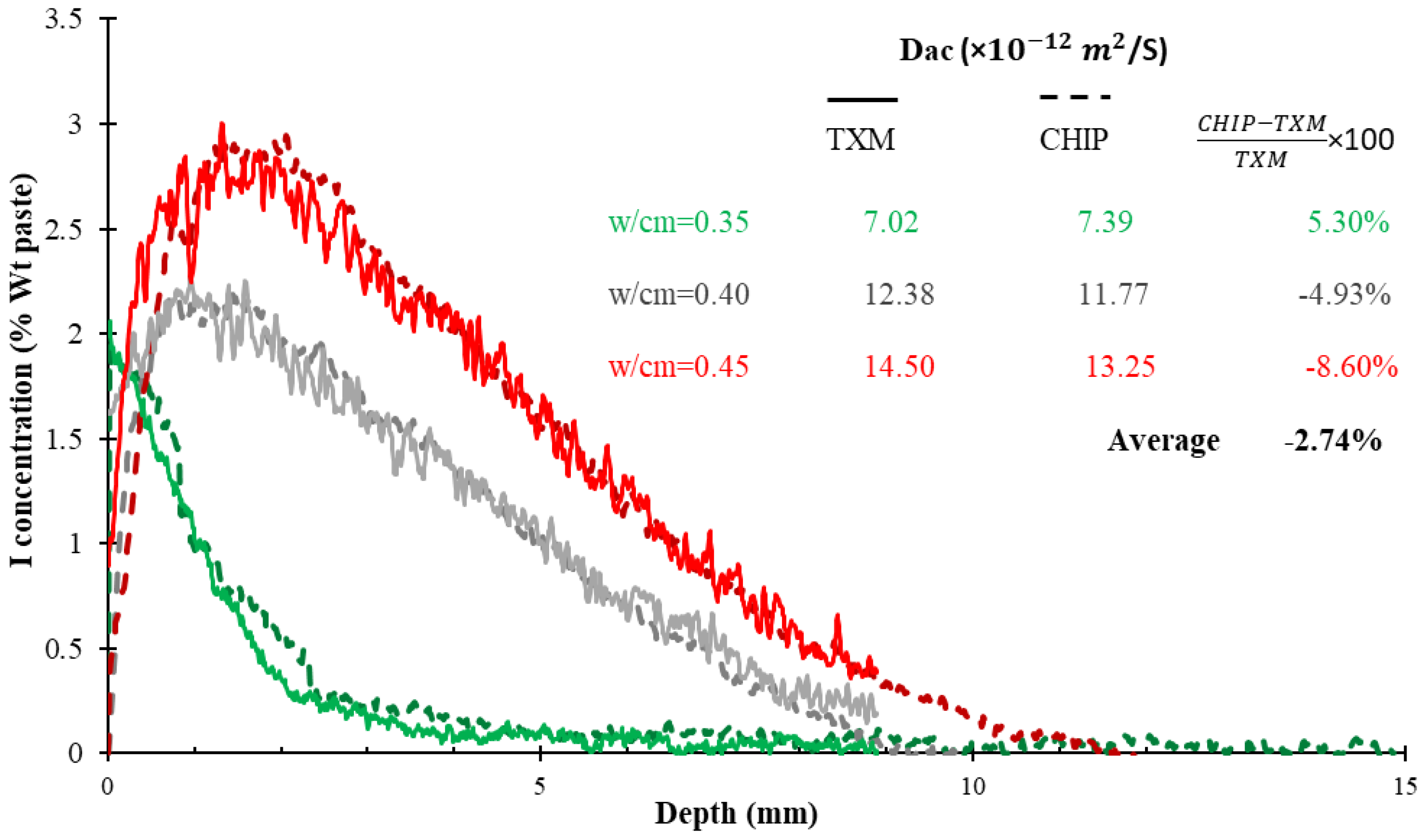
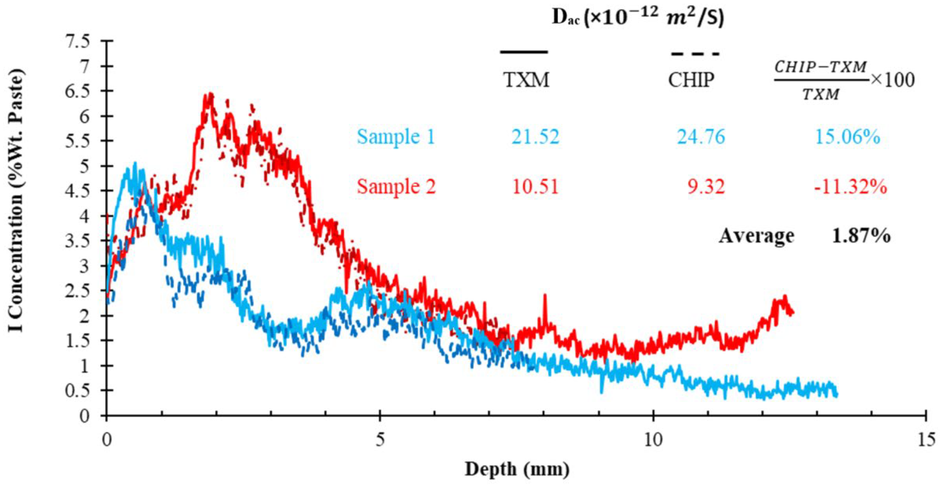
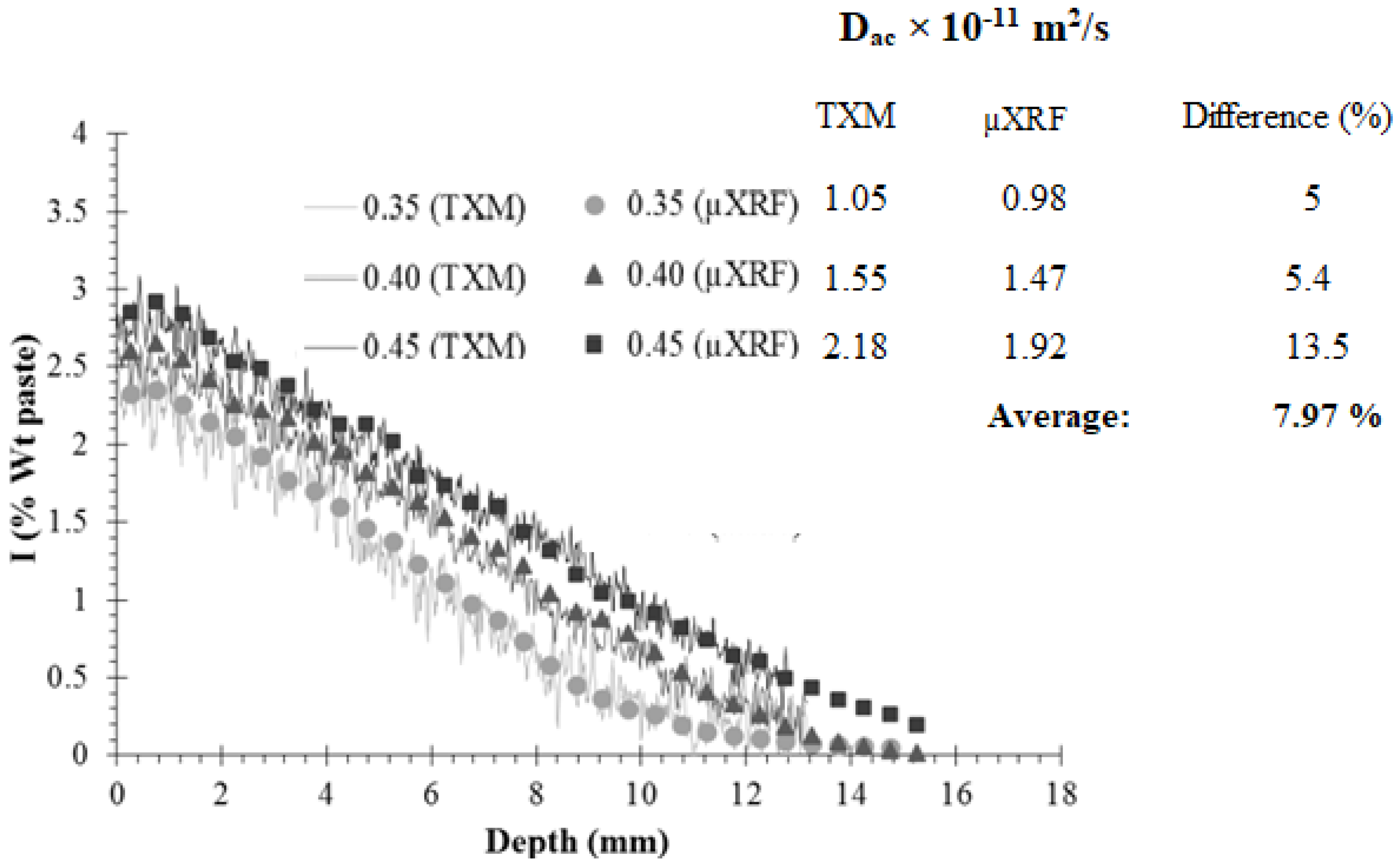
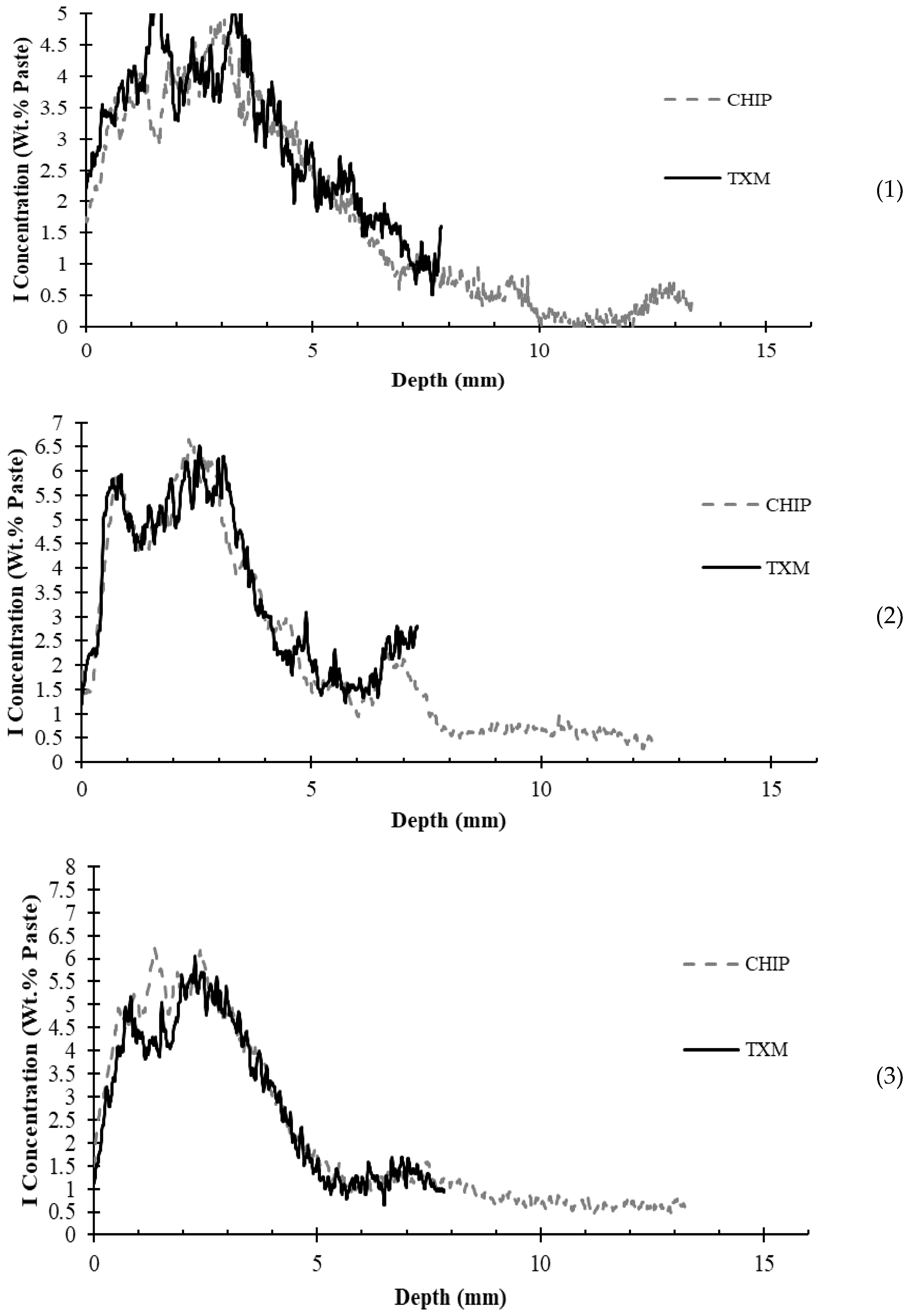
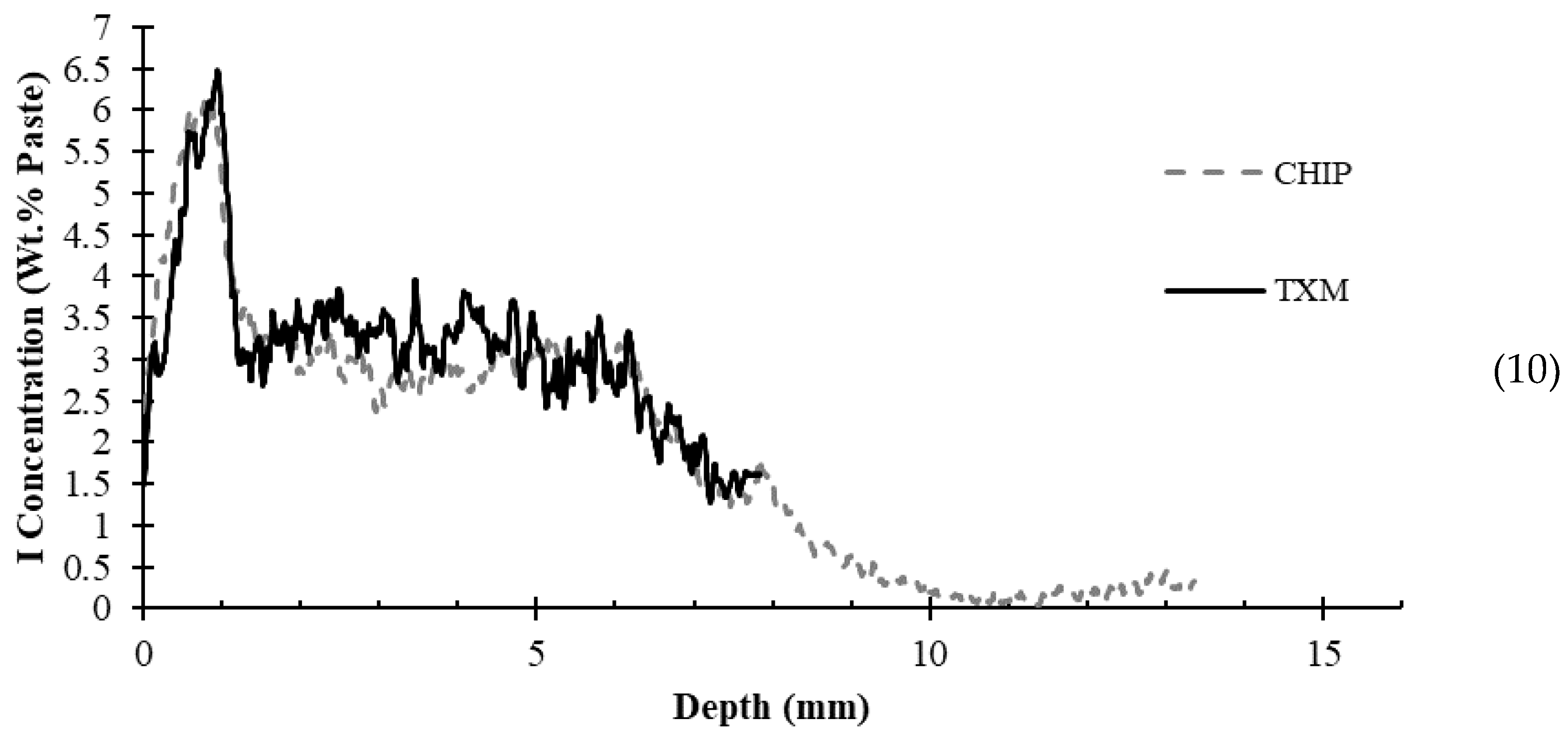
Figure 8 shows the concentration profiles of three paste samples with different w/cm ratios after 14 d of ponding for both CHIP and TXM. The TXM results are shown with a solid line, and the CHIP results are shown with a dashed line. Figure 8 shows the results are very comparable between TXM and CHIP for different w/cm ratios. The average difference in the Dac is 2.74%, and the maximum difference is 8.6%.
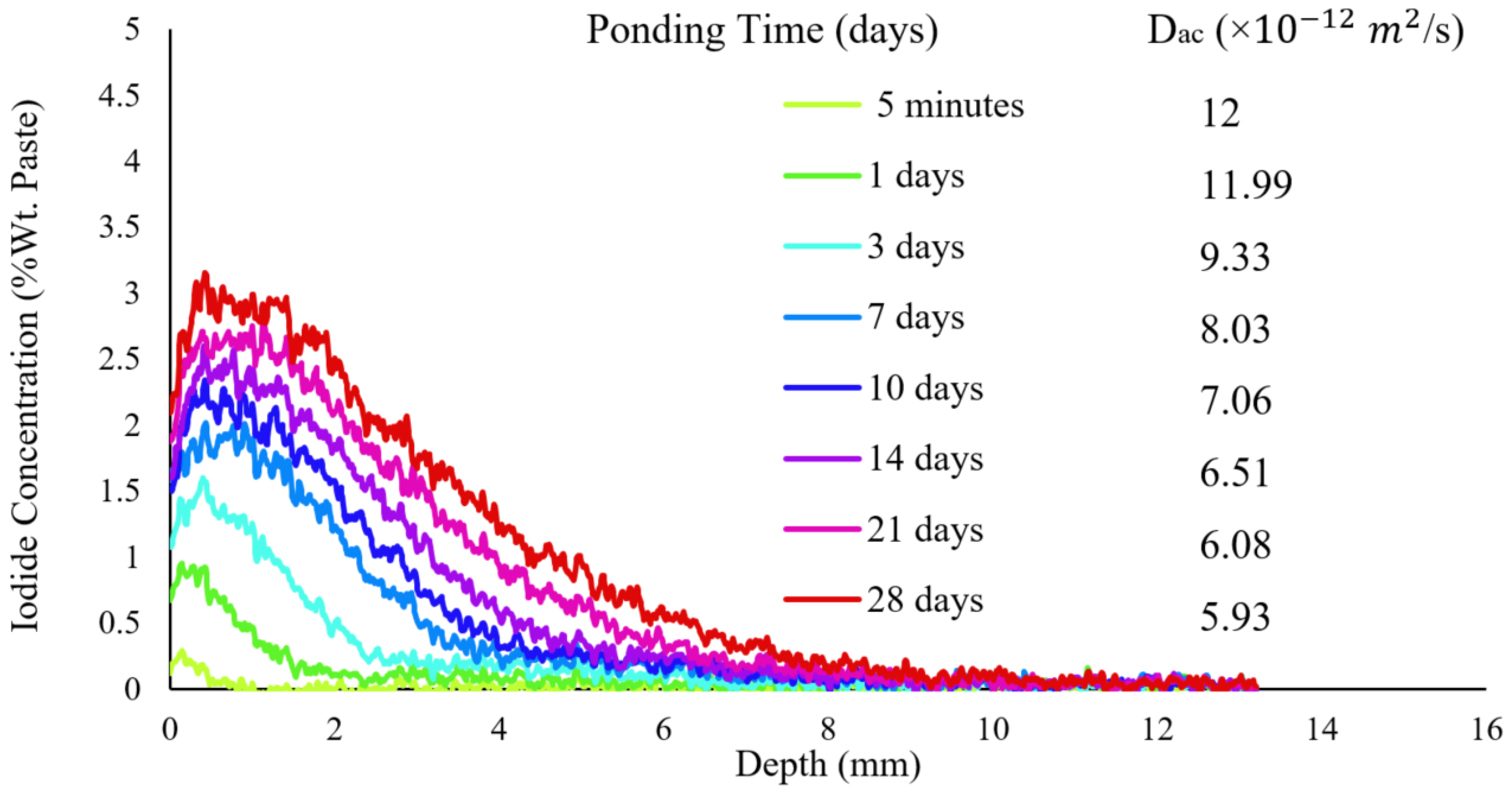
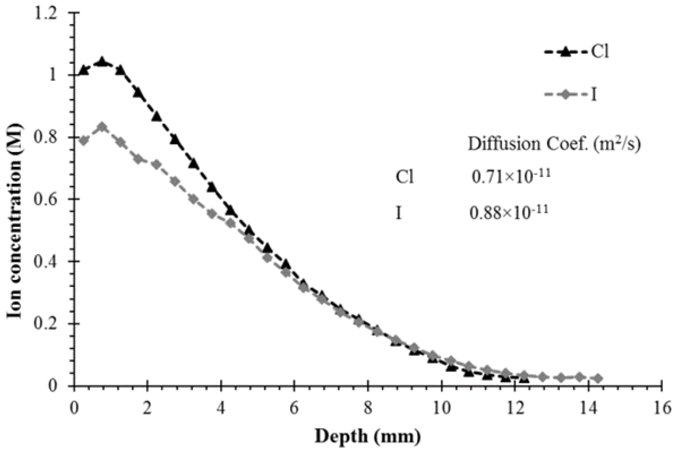
The concentration profiles shown in Figure 8 show an initial rise in chloride concentration to a maximum point (Cmax) within the first layers below the surface (Δx), followed by a gradual decrease in chloride concentration at the lower depths. This phenomenon, which is often referred to in the literature as the “maximum phenomenon”, can be attributed to several reasons [27,41,42,43,44,45,46]: first, chlorides can be leaching from the cement paste; second, chlorides can move into the outer layer of concrete by convection and not necessarily by diffusion; third, there is variability in microstructure in surface compared to the deeper depths; forth, maximum concentration (Cmax) has time-variant characteristics that increase non-linearly with the exposure duration, while the exposure duration has minimal impacts on Δx. In addition, the concentration of the exposure environment is found to be a significant factor influencing both Cmax and Δx [41].
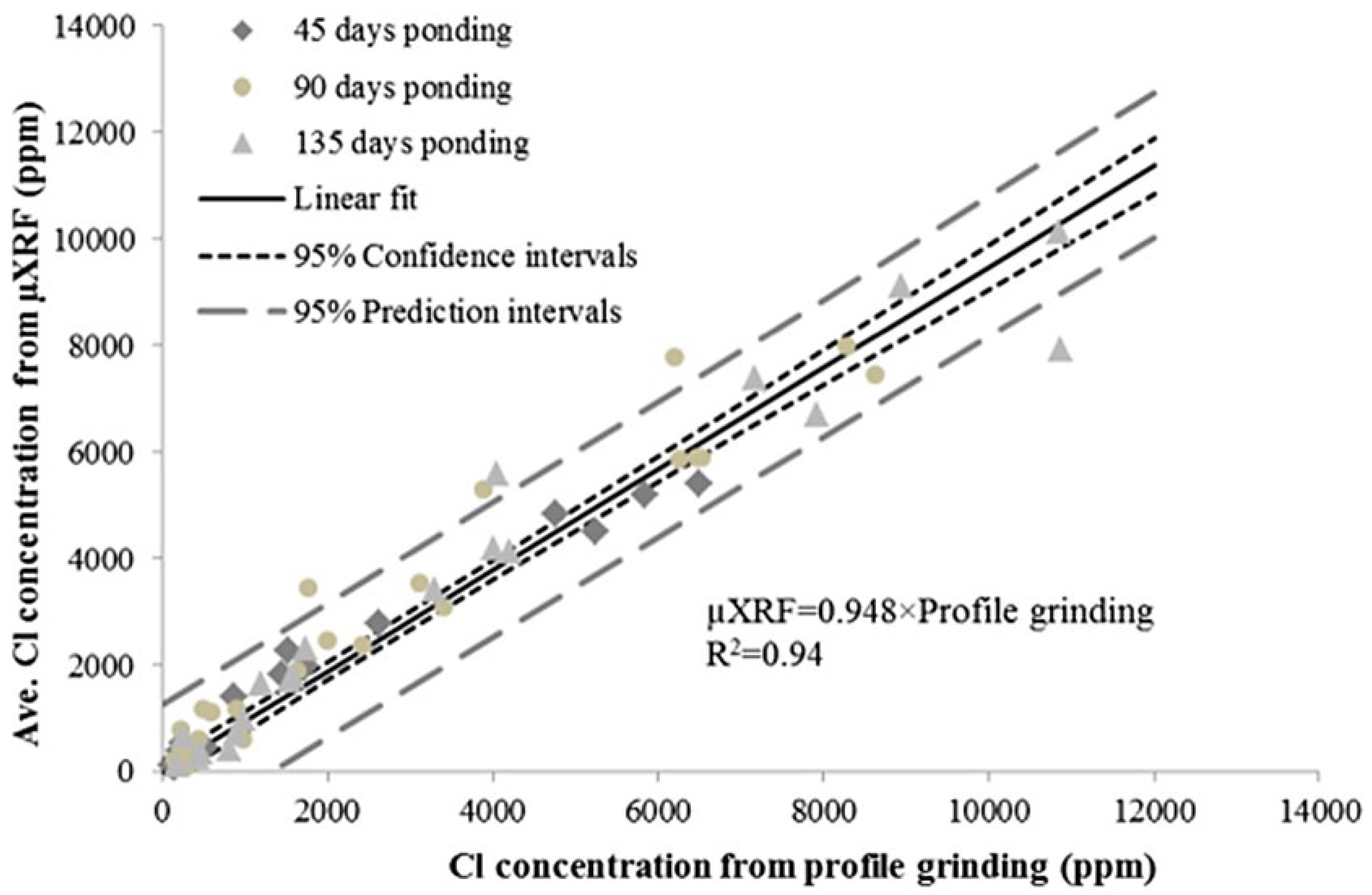
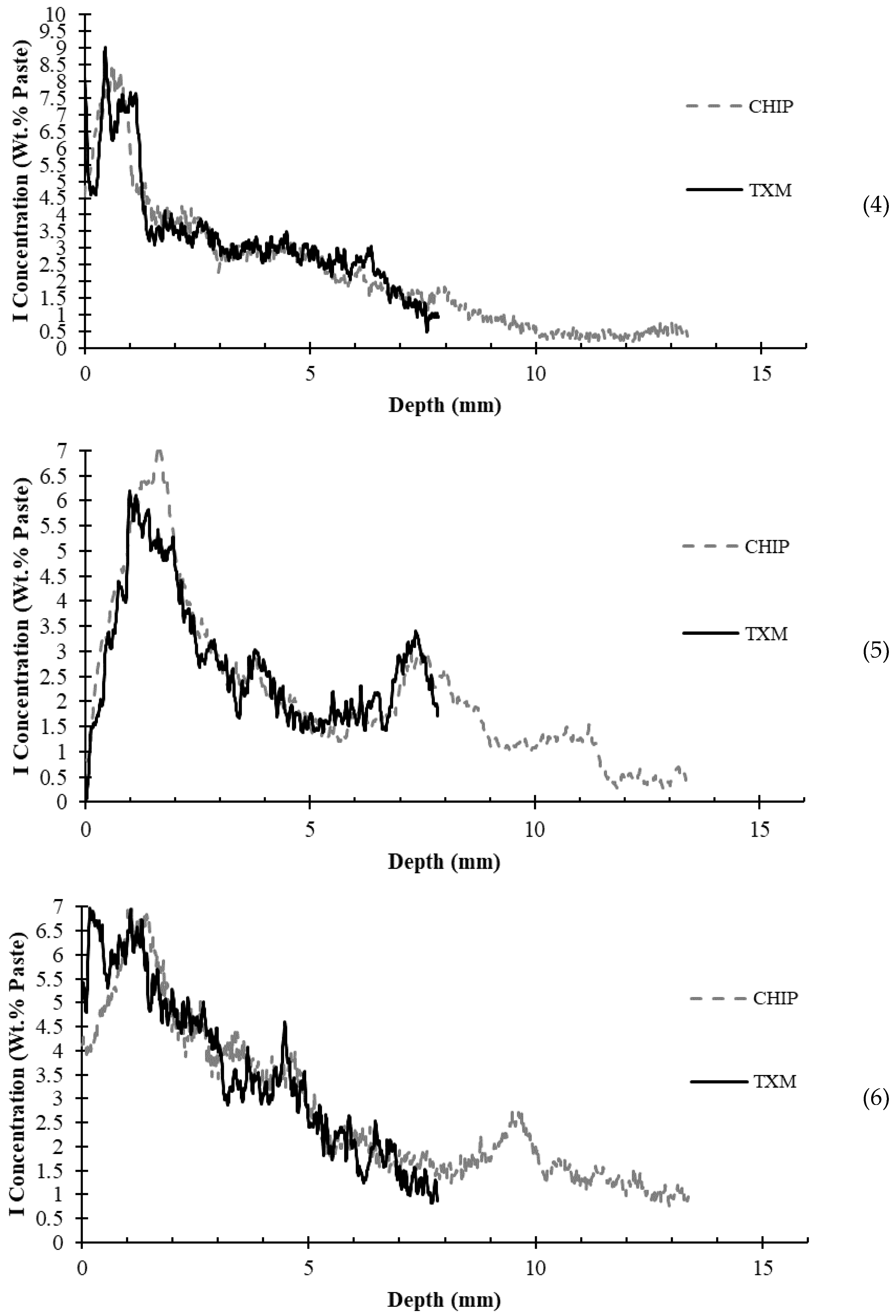
The 12 concrete samples were tested with both CHIP and TXM, and Figure 9 shows the concentration profiles of the two samples in both methods. The other results can be found in Appendix E. The higher amount of variability in the concrete samples may be caused by minor differences in the sample loading in the two X-ray machines that could magnify any anomalies in the sample caused by aggregates. Additionally, the diffusion coefficient calculation assumes that the concentration profile has a certain shape. If the results do not meet this shape, then small changes can cause the curve fit to be unstable and produce different results. This is being addressed further for future publications.
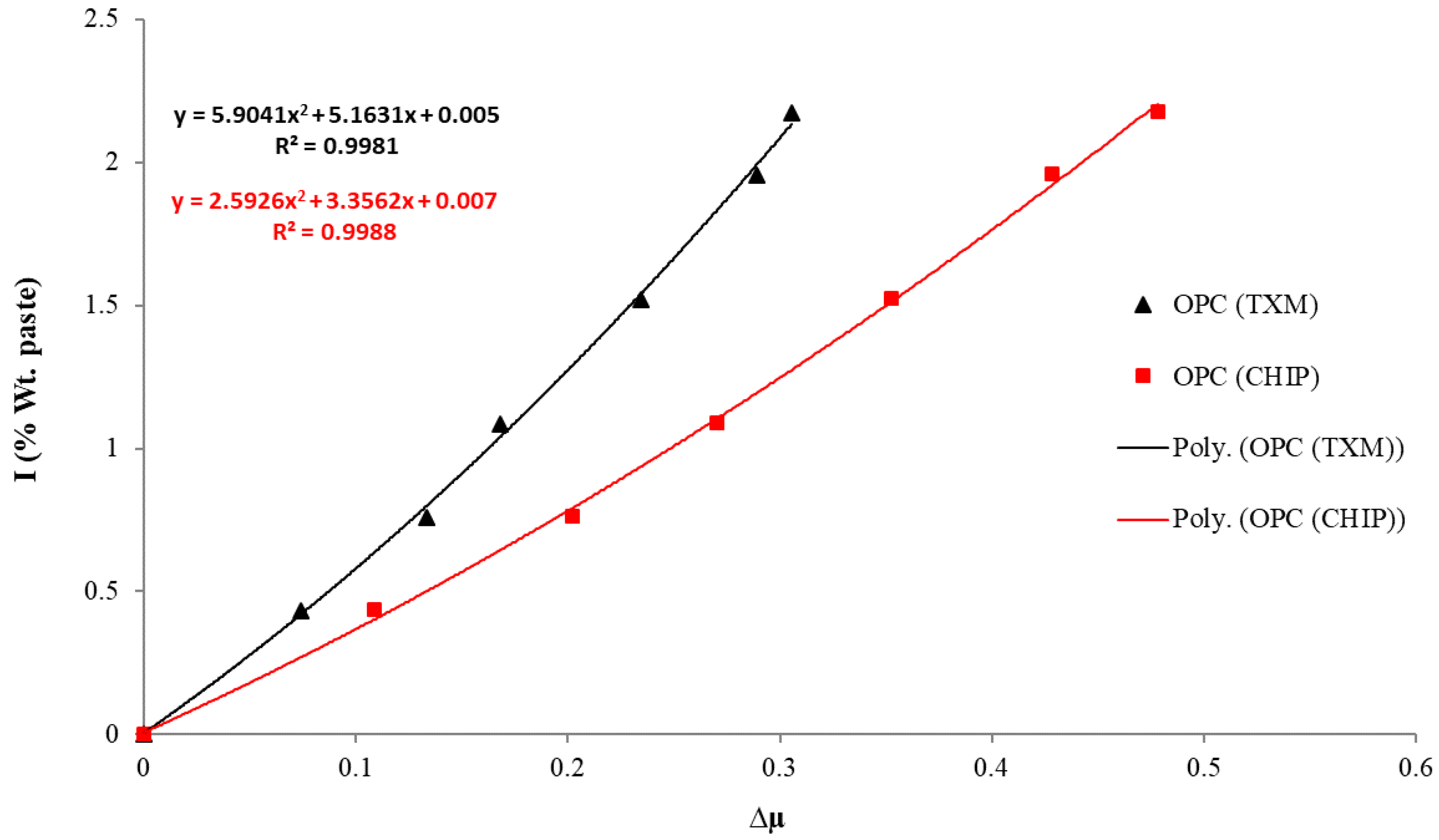
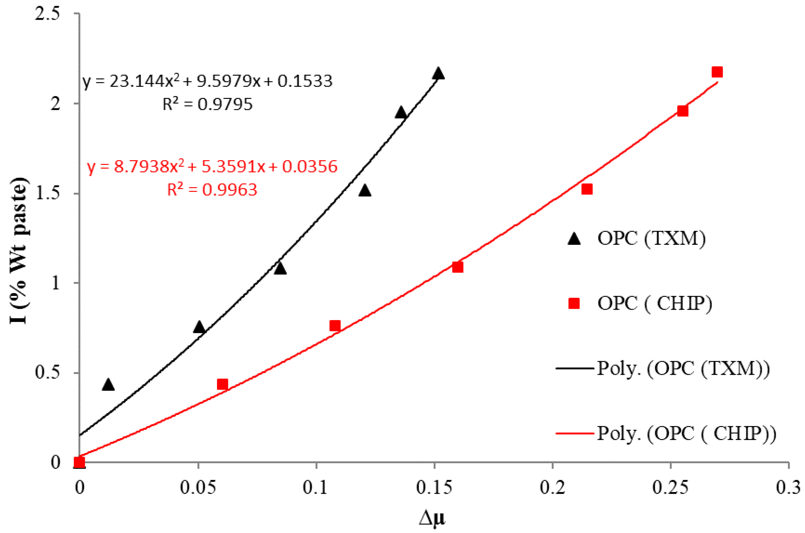
To compare the diffusion coefficients obtained by both CHIP and TXM techniques, the results from twenty-four paste samples and twelve concrete samples are presented in Figure 10. The average percent difference of the measured Dac between the two measurement methods is 1.02%, with a maximum difference of 16.9%. The 95% prediction intervals are shown with a blue dashed line in Figure 10. A 95% prediction interval is an estimate of the range where a future observation will fall with a 95% probability. For these data, all of the observations are within the 95% prediction interval. Linear regression was plotted with these data observations in Figure 10. The slope of the linear regression line is 0.986, which is close to the ideal slope of 1.00, and the R2 value is 0.99. This shows that linear regression is appropriate for the data. This means that the results of CHIP and TXM are comparable.

4.2. Repeatability of the CHIP Procedure for Concrete

Since concrete is a non-homogenous material and the sample size is limited, it is important to understand the variability of the measurements obtained by CHIP. Two approaches were considered to evaluate the variation of CHIP. The same concrete core was repeatedly scanned to evaluate the reproducibility of CHIP, and then the cores were investigated from different angles.
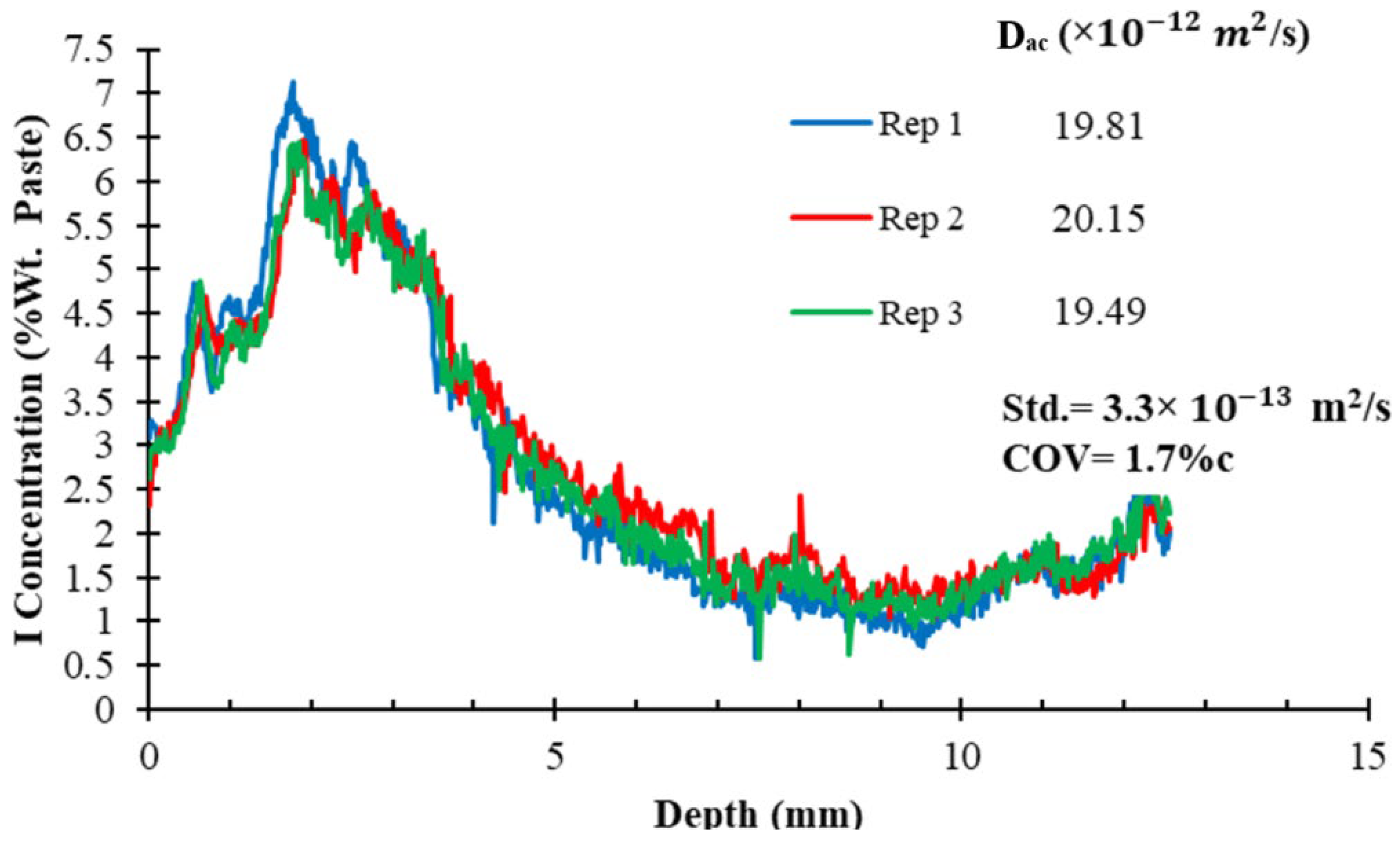
To evaluate the precision of the CHIP, a concrete sample was loaded, scanned, and removed from the machine. This was repeated three times for each sample. The results are shown in Figure 11, and the results of all 12 concrete samples are summarized in Table 5. The results of every single measurement are reported in Appendix F. Results in Figure 11 and Table 5 show the strong repeatability of the experiment by a single user with a standard deviation of 3.07 × 10⁻¹³ m2/s and a coefficient of variation (COV) of 1.78%. This shows that CHIP can be used to produce highly reproducible measurements of ion penetration for repeat measurements on the same sample at the same orientation.
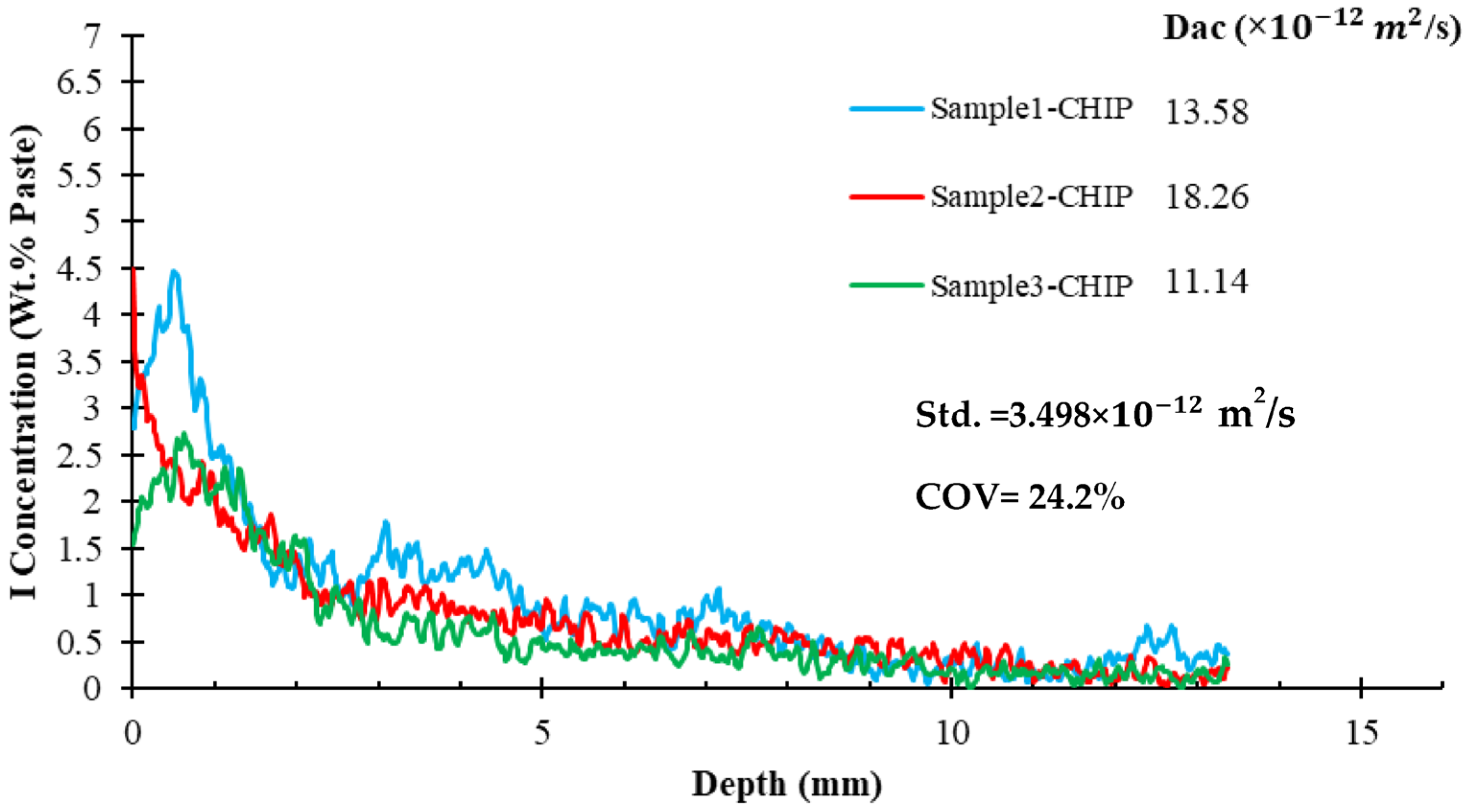
Next, three cores were taken from the same concrete sample, and all three cores were scanned from a single direction. This approach examines the variation of repeat measurements from the same larger sample. The results of this evaluation are shown in Figure 12. The standard deviation and coefficient of variation (COV) were equal to 3.498 × 10⁻¹² m2/s and 24.2%, respectively. The higher variability of the concrete samples compared to the paste samples is likely due to the more inhomogeneous nature of the concrete samples. The COV of 24.2% in CHIP is higher than the COV of 14.2% for the single-laboratory repeatability of ASTM C 1556.
This higher level of variability for CHIP could be caused because the analysis uses a region of 0.88 mm to minimize any cupping artifacts. Since concrete is a composite material, considering only a narrow strip in the center of each radiograph during data analysis may be impacted by variations in the aggregate found in the concrete samples. This means that different samples will have a different distribution of paste and aggregates in the central region of each radiograph at each angle. This will have an impact on the results. For this reason, the authors suggest taking radiographs at different angles of a concrete sample, then calculating the Dac attributed to each angle and reporting the average Dac for each concrete sample. Another solution can be using cubic-cut samples instead of cored samples to eliminate cupping artifacts and then consider a larger area for data analysis.
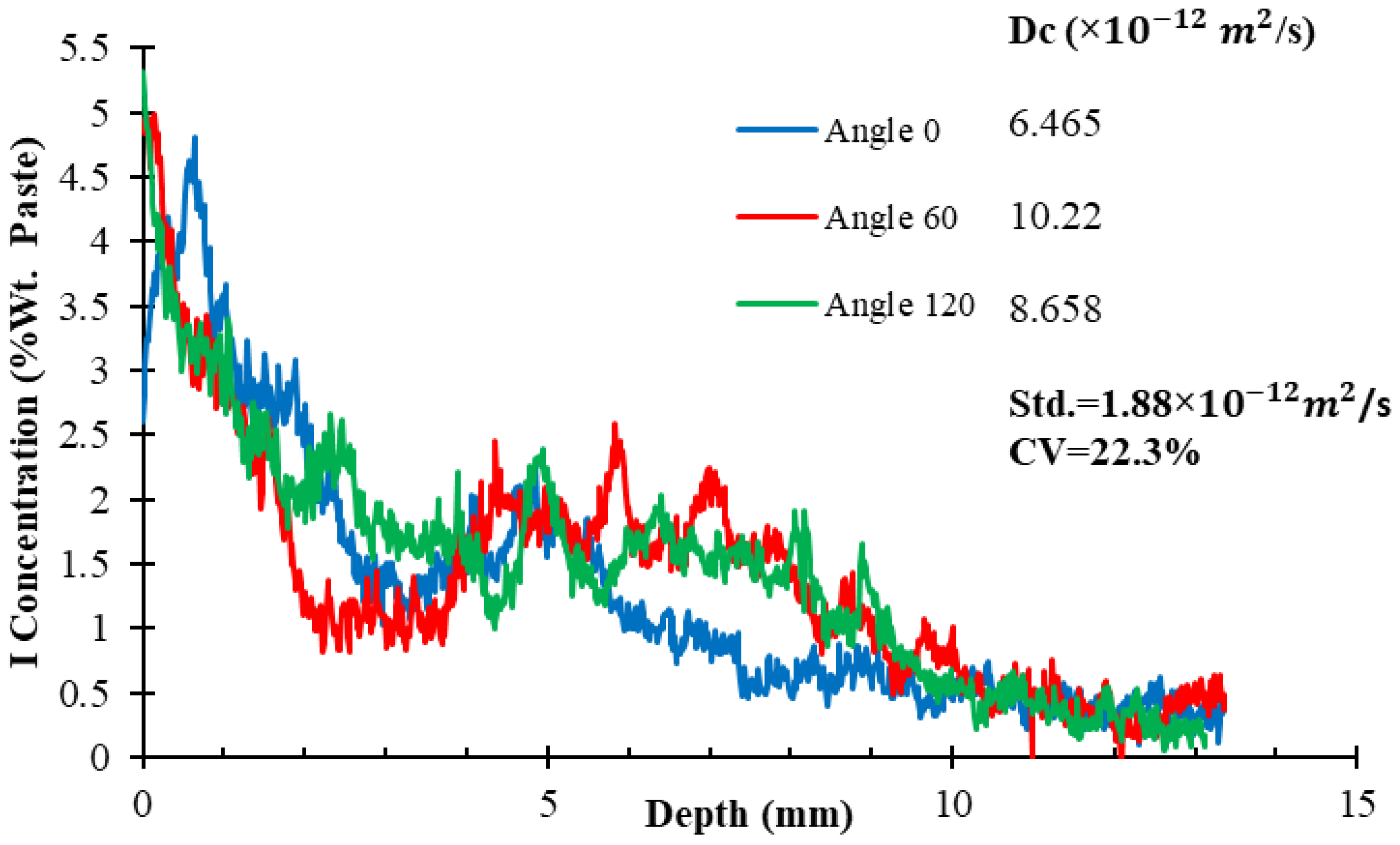
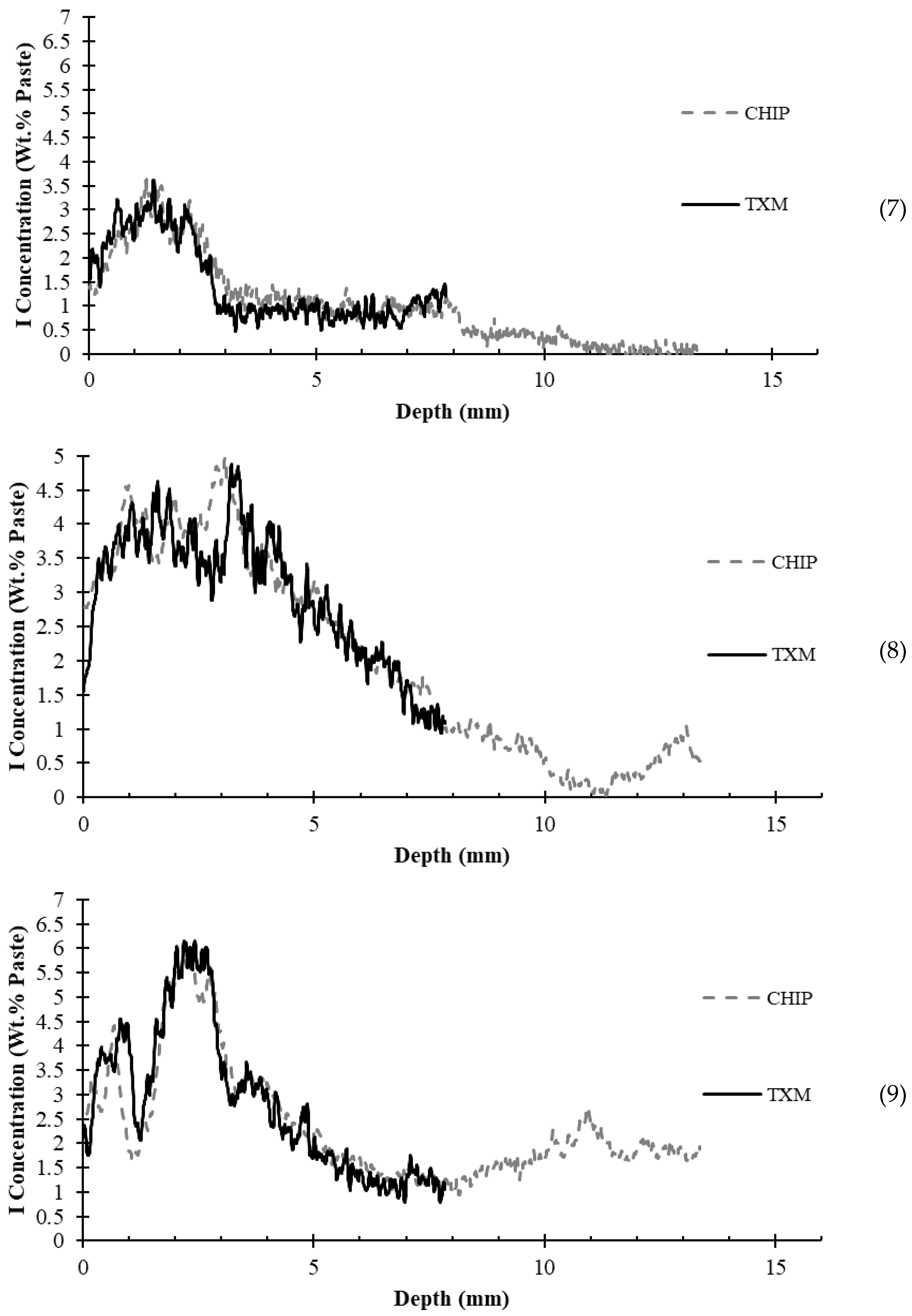
The discussion above brings up a concern about the importance of scan direction in CHIP. To determine the impact of the direction of scanning on diffusion results for concrete samples, each sample was scanned from the angles of 0°, 60°, and 120°. The results of one sample are shown in Figure 13, and the results of all tested samples are reported in Table 6. More details are reported in Appendix G. The reader must remember that only the center of 0.88 mm of each radiograph was analyzed. This means that these samples will have a different distribution of paste and aggregates in the central region of each radiograph at each angle. This will have an impact on the results. While the concentration profiles in Figure 13 showed similar trends, the COV is 22.3%. As shown in Table 6 the average value of COV for all 12 concrete samples is equal to 23.43%. This is similar to the COV found in Figure 12 for three different samples from the same concrete cylinder. This means that the variability from three different angles on the same sample is similar to the variability from three different samples from the same mix.
One way to overcome this variability is to take radiographs from an even larger number of angles and use the average concentration to calculate the Dac. Each of these concentration profiles gives a Dac, and this could help determine how homogeneous the sample is from different angles. Larger samples could also be investigated so that more material can be investigated. Additionally, a wider investigation window could be used by accounting for the cupping artifacts in the scan. These are all areas of future work.

4.3. COV and ANOVA Analysis of the CHIP Samples at Different w/cm Ratios

The coefficient of variance (COV) of the 27 paste samples per w/cm of 0.35, 0.40, and 0.45 was calculated as 11.3%. 12.1%, and 16.8%, respectively. The average standard deviation (Std.) and COV for the Dac values calculated for all 81 paste samples (27 samples per each w/cm) tested with CHIP were equal to 1.38 × 10⁻¹² m2/s and 13.4%, respectively. The 95% confidence interval of COV for the paste samples in CHIP showed a lower limit of 7.46% and an upper limit of 19.34%, which shows that all three COV values of the paste samples are not significantly different for the different w/cm ratios. This means that the variation of the measurements for the paste samples does not change significantly at different w/cm ratios.
Another way to determine if the different w/cm ratios are statistically significant, the ANOVA analysis, is shown in Table 7. By accepting a 5% significance level, p < 0.05 rejects the null hypothesis. When p < 0.05, it shows that there is a significant difference between the Dac of three groups with different w/cm ratios. In other words, CHIP can show that the Dac of the paste samples changes by changing the w/cm between 0.35, 0.40, and 0.45. It is worth noting that the Dac values for the tested w/cm are significantly different.

5. Practical Implications

The CHIP technique is a useful, repeatable, and non-destructive technique to determine the Dac for the samples investigated. The results can also be obtained within 14 d instead of the 35 d required with ASTM C1556, and the test requires minimal sample preparation and user time. CHIP provides the Dac, which is a direct measurement of a key durability property of a concrete mixture. The Dac could also be measured on samples from either the laboratory or taken from the field. In addition, to all of these benefits, the test method can be completed with dental equipment that is widely available. Because the equipment is so widely available, this makes this technique promising. This could create a new opportunity to measure the in-place properties of concrete infrastructure promptly and help guide construction practices to ensure that durable concrete is produced. This could help ensure the long-term durability of the concrete infrastructure and reduce repairs.
CHIP can also be used to investigate the performance of service structures and determine the efficiency of surface coatings [47]. CHIP can also be used to study ion transport in complex geometries such as cracked concrete or concrete being deteriorated by other durability mechanisms. Finally, the results obtained from these measurements can be used to predict the service life of a structure to effectively plan for maintenance and repair cycles.

6. CHIP Limitations

While CHIP shows significant promise, the technique has limitations. For example, the method cannot detect materials with low electron density like water. Additionally, the scans must be well aligned to make sure that the changes in the sample can be determined over time. The biggest limitation of the method is that it requires calibration curves to be used. These calibration curves are somewhat sensitive to the materials being used. Currently, the variation of the test method is high as discussed in Section 4.2; however, there is current research being completed to address this.

7. Conclusions

For this investigation, a novel test method to determine the apparent diffusion coefficient of ion penetration into concrete materials was developed called checking ion penetration (CHIP). The following results can be concluded from this work:
  • CHIP can determine the apparent diffusion coefficient by measuring the ion penetration through both paste and concrete by using an iodide ponding solution.
  • When comparing CHIP and TXM, the average difference between the apparent diffusion coefficients (Dac) for paste and concrete is 1.02%.
  • Using CHIP, the average standard deviation (Std.) and coefficient of variance (COV) for the Dac values calculated for all paste samples are equal to 1.38 × 10⁻¹² m2/s and 13.4%, respectively, while the Std. and COV values for concrete samples are equal to 3.498 × 10⁻¹² m2/s and 24.2%, respectively. The higher variability values of the concrete samples compared to the paste samples is likely due to the inhomogeneity nature of the concrete samples.
  • CHIP is highly repeatable by a single user with an Std. of 3.07 × 10⁻¹³ m2/s and COV equal to 1.78%.
These results show that CHIP is a promising test method to rapidly evaluate the ion penetration of cementitious materials. Since CHIP uses widely available dental X-ray equipment then it may serve as a valuable tool in many countries to evaluate the durability of concrete infrastructure.

Author Contributions

Conceptualization, M.T.L. and Q.H.; Methodology, A.B., M.T.L., D.C., Q.H. and R.B.; Formal Analysis, A.B.; Investigation, A.B., Q.H. and A.R.; Data Curation, A.B., Q.H. and A.R.; Writing—Original Draft Preparation, A.B.; Writing—Review and Editing, A.B., D.C. and M.T.L.; Supervision, M.T.L.; Project Administration, M.T.L.; Funding Acquisition, M.T.L. All authors have read and agreed to the published version of the manuscript.

Funding

This research was funded by National Cooperative Highways Research Program—Innovations Deserving Exploratory Analysis (NCHRP-IDEA) program Project 199.

Data Availability Statement

The data presented in this study are available on request from the corresponding author.

Acknowledgments

The authors acknowledge the financial support of NCHRP-IDEA Project 199 and the research oversight panel. The authors would like to thank Ali Hendi for giving valuable feedback and comments. In addition, the authors would like to thank Hadi Bolooki Pursaheli for his assistance in providing schematic pictures.

Conflicts of Interest

The authors declare no conflict of interest.

Appendix A. Validation of TXM Technique

The first concern about the reliability of the developed technique is to what extent iodide can represent chloride. Khanzadeh et al. [27] compared the concentration profile and diffusion coefficients of the paste sample with w/cm of 0.4 after 28 d ponding with 0.6 M KI and 0.6 M NaCl solutions. They used the micro-X-ray fluorescence (µXRF) technique for their observations. µXRF is a non-destructive method that uses direct X-ray excitation to induce characteristic X-ray fluorescence emission from the sample to collect spatially resolved maps of chemical concentrations.
As shown in Figure A1, for approximately the first 30% of the penetration depth, iodide concentration was higher, but about 70% of both profiles match. Iodide showed a 24% higher diffusion coefficient compared to chloride. Overall, iodide serves as a satisfactory tracer to represent the diffusion and penetration of chloride in a cementitious system.
Figure A1. Comparison of iodine and chloride concentration profiles [27].
Civileng 04 00014 g0a1
Khanzadeh et al. [27] compared findings between TXM and µXRF. They tested paste samples with different w/cm ratios of 0.35, 0.4, and 0.45 with both TXM and µXRF, as shown in Figure A2. Results showed that the diffusion coefficient of TXM on average is 8% higher than µXRF. Khanzadeh et al. by statistical analysis proved that TXM and µXRF provide statistically comparable results.
Figure A2. Comparison of TXM results with µXRF [27].
Civileng 04 00014 g0a2
Khanzadeh et al. [17] examined the validity of µXRF by comparing µXRF to a very well-known grinding technique described in ASTM C1556 [11]. They made concrete samples and after curing them, ponded the samples with 165 g/L aqueous sodium chloride solution for either 45, 90, or 135 d at 23 °C. When the solution was removed, the samples were powdered at 1–5, 5–10, 10–15, and 15–20 mm depths parallel to the exposed surface. After the powder was collected, the remaining sample was split and the exposed cross-section was polished to prepare the samples for µXRF imaging. Figure A3 compares the individual measurements from the profile grinding to the average μXRF values over the same depths. The slope of the linear trend line is 0.948, which is close to the ideal value of 1, with the μXRF data being slightly lower on average than the data from the profile grinding.
To recapitulate, it has been shown that μXRF gives comparable results to profile grinding, which is a direct observation and accepted testing method of obtaining chloride concentration profile at each depth of a cementitious system. Furthermore, it has been shown that iodide can be an acceptable representative of chloride. Therefore, it has been shown that iodide concentration profiles obtained by both TXM and μXRF are comparable, and since μXRF has been validated by profile grinding, then TXM can be considered a reliable technique. This study tried to validate the reliability of CHIP by comparing the results to TXM as an already established and reliable technique.
Figure A3. Correlation between results from μXRF and profile grinding [17].
Civileng 04 00014 g0a3

Appendix B. Mix Designs of Concrete Samples Cored from Bridge Decks

Table A1. Mix design of field concrete samples.
SampleCoarse AggregateFine AggregateCementAir Content %Fly AshWater (Kg/m3)Water Reducer (ASTM C-494 Type A/D)Air-Entrainer (ASTM C-260)w/b
Ratio
NameSpecific GravityKg/m3Specific GravityKg/m3Kg/m3TypeSpecific GravityKg/m3TypeSpecific GravityKg/m3Specific GravityKg/m3
1#672.691097.62.62730.9334.66NONE148.3A351.010.891.000.1770.44
2#672.691067.92.62709.0362.56NONE158.4A361.011.91.000.0590.44
3#672.691073.82.62717.9290.16C2.6572.4148.3A381.011.421.000.1190.41
4Not Provided
5
6#672.671072.02.62714.3290.16C2.6572.4148.3A381.011.421.000.1190.41
7#572.651020.42.63777.2334.66.5% ± 1.5%NONE148.3A36Not Provided0.44
8#672.691097.62.62730.9334.66NONE148.3A351.010.891.000.1770.44
9#672.671067.92.62709.0362.56NONE158.4A361.011.91.000.0590.44
10Not Provided

Appendix C. Image Processing on Raw Images Obtained from CHIP

To be able to compare the images from the two methods, the CHIP images had to be transformed to match the gray value range of the TXM method. To do this, a software programming code [37] was prepared to import each image, process the image, and write the output image in BMP format. Equation (A1) was used in the programming code to normalize the gray values in the raw image of CHIP and transform the gray values range of CHIP to the gray values range of TXM.
GV =     G V d Min Max Min
where GVi is the gray value of the processed image, GVd is the gray value of each pixel in the raw CHIP radiograph (TIFF format), and Max and Min are the maximum and minimum gray values in the captured radiographs, respectively. In this study, the Max and Min in the TIFF images were equal to 4500 and 75, respectively. The reason for having Max and Min values different from the ultimate Max and Min values (6500 and 0) is that in the captured radiographs there was not any pure black or pure white.

Appendix D. Calibration Curve

Calibration curves help to convert attenuation values (Δµ) to concentration values. To develop the calibration curves for both TXM and CHIP methods, standard samples with known iodide concentrations were made by adding different iodide concentrations to the mixtures during mixing. Then these samples were scanned and analyzed as stated in Section 3.4 and Section 3.5. After scanning the standard samples, the attenuation related to each concentration was extracted. Ultimately, a polynomial curve of order 2 was fitted on the obtained spots to obtain an equation that converts the attenuation to the concentration. Figure A4 and Figure A5 show the calibration curves obtained by the two methods for paste and mortar, respectively. The mortar calibration curve was used to return the concentration values in concrete samples.
Figure A4. Calibration curve for paste (w/cm = 0.4) that was used to calculate concentrations in concrete samples.
Civileng 04 00014 g0a4
Figure A5. Calibration curves for mortar (w/cm = 0.4) that was used to calculate concentrations in concrete samples.
Civileng 04 00014 g0a5

Appendix E. Comparison of TXM and CHIP Concentration Profiles for All Other 10 Concrete Samples

Figure A6. Comparison of TXM and CHIP concentration profiles for all other 10 concrete samples. The numbers next to each graph, show the sample name.
Civileng 04 00014 g0a6aCivileng 04 00014 g0a6bCivileng 04 00014 g0a6cCivileng 04 00014 g0a6d

Appendix F. Diffusion Coefficient of 12 Concrete Samples Tested Three Times from the Same Side

Table A2. Diffusion coefficient of 12 concrete samples tested three times from the same side (Dac × 10−12 m2/s).
RepetitionSample 1Sample 2Sample 3Sample 4Sample 5Sample 6Sample 7Sample 8Sample 9Sample 10Sample 11Sample 12
Rep 110.399.4820.5127.6419.688.8829.7718.4019.8116.8312.2813.10
Rep 210.739.2120.0127.2218.988.8230.9218.4020.1517.0912.5613.55
Rep 310.579.5819.9027.2819.688.8330.9218.8319.4916.2012.9012.91
Average10.569.4220.1727.3819.458.8530.5318.5519.8216.7012.5813.18
Std.0.170.190.310.230.410.030.670.250.330.460.310.33
COV (%)1.612.061.530.832.100.342.181.351.672.772.452.50
Average of COV1.78%

Appendix G. Diffusion Coefficient of 12 Concrete Samples Tested from Three Angles

Table A3. Diffusion coefficient of 12 concrete samples tested from three angles (Dac × 10−12 m2/s).
AngleSample 1Sample 2Sample 3Sample 4Sample 5Sample 6Sample 7Sample 8Sample 9Sample 10Sample 11Sample 12
Angle 013.5621.9819.7632.646.4734.5754.6917.7524.4825.0148.4217.42
Angle 6017.7018.5426.6749.9210.2220.5856.7723.6617.8514.2547.6915.05
Angle 12015.7911.6220.0921.518.6613.9073.3626.1716.2618.9136.8814.43
Average15.6917.3822.1734.698.4523.0261.6122.5219.5319.3944.3315.64
Std.2.075.273.9014.321.8910.5510.234.324.365.406.461.58
COV (%)13.2230.3417.5941.2722.3345.8316.6119.1922.3327.8314.5810.08
Average of COV23.43%

References

  1. Hilsdorf, H.; Kropp, J. Performance Criteria for Concrete Durability; CRC Press: Boca Raton, FL, USA, 1995. [Google Scholar]
  2. Riding, K.A.; Poole, J.L.; Schindler, A.K.; Juenger, M.C.G.; Folliard, K.J. Simplified concrete resistivity and rapid chloride permeability test method. ACI Mater. J. 2008, 105, 390–394. [Google Scholar]
  3. Shi, X.; Xie, N.; Fortune, K.; Gong, J. Durability of steel reinforced concrete in chloride environments: An overview. Constr. Build. Mater. 2012, 30, 125–138. [Google Scholar] [CrossRef]
  4. Feldman, R.; Prudencio, L.R., Jr.; Chan, G. Rapid chloride permeability test on blended cement and other concretes: Correlations between charge, initial current and conductivity. Constr. Build. Mater. 1999, 13, 149–154. [Google Scholar] [CrossRef]
  5. Wee, T.H.; Suryavanshi, A.K.; Tin, S.S. Evaluation of rapid chloride permeability test (RCPT) results for concrete containing mineral admixtures. Mater. J. 2000, 97, 221–232. [Google Scholar]
  6. Shi, C.; Stegemann, J.A.; Caldwell, R.J. Effect of supplementary cementing materials on the specific conductivity of pore solution and its implications on the rapid chloride permeability test (AASHTO T277 and ASTM C1202) results. Mater. J. 1998, 95, 389–394. [Google Scholar]
  7. Sengul, O. Use of electrical resistivity as an indicator for durability. Constr. Build. Mater. 2014, 73, 434–441. [Google Scholar] [CrossRef]
  8. Polder, R.B. Test methods for on site measurement of resistivity of concrete—A RILEM TC-154 technical recommendation. Constr. Build. Mater. 2001, 15, 125–131. [Google Scholar] [CrossRef]
  9. Layssi, H.; Ghods, P.; Alizadeh, A.R.; Salehi, M. Electrical resistivity of concrete. Concr. Int. 2015, 37, 41–46. [Google Scholar]
  10. Elkey, W.; Sellevold, E.J. Electrical Resistivity of Concrete; Norwegian Road Research Laboratory Publication: Oslo, Norway, 1995; Available online: https://vegvesen.brage.unit.no/vegvesen-xmlui/bitstream/handle/11250/191626/Publication%2080.pdf?sequence=1 (accessed on 16 July 2022).
  11. ASTM C1556; Standard Test Method for Determining the Apparent Chloride Diffusion Coefficient of Cementitious Mixtures by Bulk Diffusion. ASTM: West Conshohocken, PA, USA, 2016.
  12. AASHTO T 259; Resistance of Concrete to Chloride Ion Penetration. ASTM: West Conshohocken, PA, USA, 1980.
  13. ASTM C1152; Standard Test Method for Acid-Soluble Chloride in Mortar and Concrete. ASTM: West Conshohocken, PA, USA, 2012.
  14. AASHTO T260-94; Standard Method for Sampling and Testing for Chloride Ion in Concrete and Concrete Raw Materials. ASTM: West Conshohocken, PA, USA, 1994.
  15. Yang, T.; Yao, X.; Zhang, Z. Quantification of chloride diffusion in fly ash–slag-based geopolymers by X-ray fluorescence (XRF). Constr. Build. Mater. 2014, 69, 109–115. [Google Scholar] [CrossRef]
  16. Danner, T.; De Weerdt, K.; Geiker, M.R. µ-XRF–Characterisation of Chloride Ingress and Self-Healing in Cracked Concrete. Available online: https://www.researchgate.net/profile/Tobias-Danner/publication/319503585_-XRF_characterisation_of_chloride_ingress_and_self-healing_in_cracked_concrete/links/59b67f83a6fdcc7415bd4bc1/XRF-characterisation-of-chloride-ingress-and-self-healing-in-cracked-concrete.pdf (accessed on 16 July 2022).
  17. KhanzadehMoradllo, M.; Sudbrink, B.; Hu, Q.; Aboustait, M.; Tabb, B.; Ley, M.T.; Davis, J.M. Using micro X-ray fluorescence to image chloride profiles in concrete. Cem. Concr. Res. 2017, 92, 128–141. [Google Scholar] [CrossRef]
  18. Khatibmasjedi, S. Insights into the Mechanisms of Salt Scaling of High Volume Fly Ash Concrete. Master’s Thesis, Oklahoma State University, Stillwater, OK, USA, 2014. [Google Scholar]
  19. du Plessis, A.; Olawuyi, B.J.; Boshoff, W.P.; le Roux, S.G. Simple and fast porosity analysis of concrete using X-ray computed tomography. Mater. Struct. 2016, 49, 553–562. [Google Scholar] [CrossRef]
  20. Burlion, N.; Bernard, D.; Chen, D. X-ray microtomography: Application to microstructure analysis of a cementitious material during leaching process. Cem. Concr. Res. 2006, 36, 346–357. [Google Scholar] [CrossRef]
  21. Bentz, D.P.; Martys, N.S.; Stutzman, P.; Levenson, M.S.; Garboczi, E.J.; Dunsmuir, J.; Schwartz, L.M. X-ray Microtomography of an Astm C109 Mortar Exposed to Sulfate Attack. MRS Proc. 1994, 370, 77–82. [Google Scholar] [CrossRef] [Green Version]
  22. Delagrave, A.; Marchand, J.; Ollivier, J.-P.; Julien, S.; Hazrati, K. Chloride binding capacity of various hydrated cement paste systems. Adv. Cem. Based Mater. 1997, 6, 28–35. [Google Scholar] [CrossRef]
  23. Stock, S.R.; Naik, N.K.; Wilkinson, A.P.; Kurtis, K.E. X-ray microtomography (microCT) of the progression of sulfate attack of cement paste. Cem. Concr. Res. 2002, 32, 1673–1675. [Google Scholar] [CrossRef]
  24. Gallucci, E.; Scrivener, K.; Groso, A.; Stampanoni, M.; Margaritondo, G. 3D experimental investigation of the microstructure of cement pastes using synchrotron X-ray microtomography (μCT). Cem. Concr. Res. 2007, 37, 360–368. [Google Scholar] [CrossRef]
  25. Proverbio, E.; Carassiti, F. Evaluation of chloride content in concrete by X-ray fluorescence. Cem. Concr. Res. 1997, 27, 1213–1223. [Google Scholar] [CrossRef]
  26. Tidwell, V.C.; Meigs, L.C.; Christian-Frear, T.; Boney, C.M. Effects of spatially heterogeneous porosity on matrix diffusion as investigated by X-ray absorption imaging. J. Contam. Hydrol. 2000, 42, 285–302. [Google Scholar] [CrossRef] [Green Version]
  27. Khanzadeh Moradllo, M.; Hu, Q.; Ley, M.T. Using X-ray imaging to investigate in-situ ion diffusion in cementitious materials. Constr. Build. Mater. 2017, 136, 88–98. [Google Scholar] [CrossRef]
  28. Michel, A.; Pease, B.J.; Geiker, M.R.; Stang, H.; Olesen, J.F. Monitoring reinforcement corrosion and corrosion-induced cracking using non-destructive X-ray attenuation measurements. Cem. Concr. Res. 2011, 41, 1085–1094. [Google Scholar] [CrossRef]
  29. Bentz, D.P.; Hansen, K.K. Preliminary observations of water movement in cement pastes during curing using X-ray absorption. Cem. Concr. Res. 2000, 30, 1157–1168. [Google Scholar] [CrossRef]
  30. Roels, S.; van Besien, T.; Carmeliet, J.; Wevers, M. X-ray attenuation technique for the analysis of moisture flow in porous building materials. In Proceedings of the Second International Conference on Research in Building Physics, Leuven, Belgium, 14–18 September 2003; Carmeliet, J., Hens, H., Vermeir, G., Eds.; AA Balkema Publishers: Lisse, The Netherlands, 2003; pp. 151–157. [Google Scholar]
  31. Roels, S.; Carmeliet, J. Analysis of moisture flow in porous materials using microfocus X-ray radiography. Int. J. Heat Mass Transf. 2006, 49, 4762–4772. [Google Scholar] [CrossRef]
  32. Pease, B.J.; Scheffler, G.A.; Janssen, H. Monitoring moisture movements in building materials using X-ray attenuation: Influence of beam-hardening of polychromatic X-ray photon beams. Constr. Build. Mater. 2012, 36, 419–429. [Google Scholar] [CrossRef]
  33. Hasanbeigi, A.; Price, L.; Lin, E. Emerging energy-efficiency and CO2 emission-reduction technologies for cement and concrete production: A technical review. Renew. Sustain. Energy Rev. 2012, 16, 6220–6238. [Google Scholar] [CrossRef] [Green Version]
  34. ASTM C150; Standard Specification for Portland Cement. ASTM: West Conshohocken, PA, USA, 2019.
  35. ASTM C305; Standard Practice for Mechanical Mixing of Hydraulic Cement Pastes and Mortars of Plastic Consistency. ASTM: West Conshohocken, PA, USA, 2006.
  36. ASTM C511; Standard Specification for Mixing Rooms, Moist Cabinets, Moist Rooms, and Water Storage Tanks Used in the Testing of Hydraulic Cements and Concretes. ASTM: West Conshohocken, PA, USA, 2019.
  37. MATLAB (R2016a), Version 9.0.0; MathWorks, Inc.: Natick, MA, USA, 2016.
  38. Barrett, J.F.; Keat, N. Artifacts in CT: Recognition and avoidance. Radiographics 2004, 24, 1679–1691. [Google Scholar] [CrossRef]
  39. Kocsis, L.; Herman, P.; Eke, A. The modified Beer–Lambert law revisited. Phys. Med. Biol. 2006, 51, N91. [Google Scholar] [CrossRef]
  40. Cavé, L.; Al, T.; Xiang, Y.; Vilks, P. A technique for estimating one-dimensional diffusion coefficients in low-permeability sedimentary rock using X-ray radiography: Comparison with through-diffusion measurements. J. Contam. Hydrol. 2009, 103, 1–12. [Google Scholar] [CrossRef]
  41. Shakouri, M.; Trejo, D. A study of the factors affecting the surface chloride maximum phenomenon in submerged concrete samples. Cem. Concr. Compos. 2018, 94, 181–190. [Google Scholar] [CrossRef]
  42. Andrade, C.; Díez, J.M.; Alonso, C. Mathematical modeling of a concrete surface “skin effect” on diffusion in chloride contaminated media. Adv. Cem. Based Mater. 1997, 6, 39–44. [Google Scholar] [CrossRef]
  43. Andrade, C.; Climent, M.A.; De Vera, G. Procedure for calculating the chloride diffusion coefficient and surface concentration from a profile having a maximum beyond the concrete surface. Mater. Struct. 2015, 48, 863–869. [Google Scholar] [CrossRef]
  44. Zhao, Y.; Chen, C.; Gao, X.; Jin, W. Seasonal variation of surface chloride ion content and chloride diffusion coefficient in a concrete dock. Adv. Struct. Eng. 2013, 16, 395–403. [Google Scholar] [CrossRef]
  45. Bamforth, P.B. The derivation of input data for modelling chloride ingress from eight-year UK coastal exposure trials. Mag. Concr. Res. 1999, 51, 87–96. [Google Scholar] [CrossRef]
  46. Andrade, C.; Rebolledo, N.; Tavares, F.; Pérez, R.; Baz, M. Concrete durability of the new Panama Canal: Background and aspects of testing. In Marine Concrete Structures; Elsevier: Amsterdam, The Netherlands, 2016; pp. 429–458. [Google Scholar]
  47. Behravan, A.; Aqib, S.M.; Delatte, N.J.; Ley, M.T.; Rywelski, A. Performance Evaluation of Silane in Concrete Bridge Decks Using Transmission X-ray Microscopy. Appl. Sci. 2022, 12, 2557. [Google Scholar] [CrossRef]
Figure 1. Sample figuration loaded in TXM machine.
Civileng 04 00014 g001
Figure 2. (a) Hexagonal stage; (b) sample by gluing a nut at the bottom.
Civileng 04 00014 g002
Figure 3. Concrete sample figuration: (a) waxed sample, (b) nut is glued, and (c) samples submerged in the potassium iodide (KI) solution.
Civileng 04 00014 g003
Figure 4. Schematic view of the mechanism of imaging in the TXM method.
Civileng 04 00014 g004
Figure 5. Schematic view of dental X-ray imaging technique setup.
Civileng 04 00014 g005
Figure 6. Concentration profiles at different ponding times for a single paste sample.
Civileng 04 00014 g006
Figure 7. (a) Radiograph with a considered region in data analyzing and (b) averaged gray value profiles.
Civileng 04 00014 g007
Figure 8. Comparing the TXM and CHIP results for paste samples with different w/cm ratios.
Civileng 04 00014 g008
Figure 9. Comparison of TXM and CHIP concentration profiles for two different concrete samples.
Civileng 04 00014 g009
Figure 10. Comparison between TXM and CHIP diffusion coefficients for all tested samples.
Civileng 04 00014 g010
Figure 11. Concentration profiles of one concrete sample after scanning one side three times.
Civileng 04 00014 g011
Figure 12. Variability of three concrete observations in the CHIP method.
Civileng 04 00014 g012
Figure 13. Concentration profiles of one concrete sample after scanning from three angles.
Civileng 04 00014 g013
Table 1. Type and number of samples used in each part of the study.
Sample Type Used for Each Part of the StudyPaste w/cm = 0.35Paste w/cm = 0.40Paste w/cm = 0.45Concrete Core
Part I: Establishing CHIP
(tested with both TXM and CHIP)
88812
Part II: Variability study of CHIP (tested only by CHIP)27272712
Table 2. Chemical composition of cement with bulk XRF (% weight).
SiO2Al2O3Fe2O3CaOMgOSO3K2ONa2OP2O5TiO2Mn2O3SrOZnOCr2O3LOI
17.394.874.7165.151.402.510.480.460.130.390.110.150.030.092.12
Table 3. Mixture proportions.
MixtureCement (g)Water (g)
Paste (w/cm = 0.35)891312
Paste (w/cm = 0.40)891354
Paste (w/cm = 0.45)891401
Table 4. Settings used in TXM and CHIP imaging techniques.
ParameterTXMCHIP
Pixel size (μm)8.9715
Voltage (keV)100120
Current (μA)1007000
Filter0.5 mm Al + Cu1.5 mm Al *
Exposure time (s)8.258
* No additional filter was used. The dental X-ray head had an inherent 1.5 mm Al filter.
Table 5. The diffusion coefficient of 12 concrete samples tested three times from the same side (Dac × 10−12 m2/s).
Sample123456789101112
Average10.569.4220.1727.3819.458.8530.5318.5519.8216.7012.5813.18
Std.0.170.190.310.230.410.030.670.250.330.460.310.33
COV (%)1.612.061.530.832.100.342.181.351.672.772.452.50
Average of COV1.78%
Table 6. Diffusion coefficient of 12 concrete samples (Dac × 10−12 m2/s).
Sample123456789101112
Average15.6917.3822.1734.698.4523.0261.6122.5219.5319.3944.3315.64
Std.2.075.273.9014.321.8910.5510.234.324.365.406.461.58
COV (%)13.2230.3417.5941.2722.3345.8316.6119.1922.3327.8314.5810.08
Average of COV23.43%
Table 7. ANOVA analysis.
Sum of SquaresdfMean SquareFSig.p < 0.05
Between groups33.11216.558.930.000
Within groups131.61791.85 YES
Total164.7281
Disclaimer/Publisher’s Note: The statements, opinions and data contained in all publications are solely those of the individual author(s) and contributor(s) and not of MDPI and/or the editor(s). MDPI and/or the editor(s) disclaim responsibility for any injury to people or property resulting from any ideas, methods, instructions or products referred to in the content.

