
Development of Prediction Model for Rutting Depth Using Artificial Neural Network

Department of Civil Engineering, University of Texas at Tyler, Tyler, TX 75799, USA
*
Author to whom correspondence should be addressed.
CivilEng 2023, 4(1), 174-184; https://doi.org/10.3390/civileng4010011
Submission received: 18 November 2022
/
Revised: 27 January 2023
/
Accepted: 3 February 2023
/
Published: 10 February 2023
(This article belongs to the Special Issue Next Generation Infrastructure)
Abstract
:One of the most common pavement distresses in flexible pavement is rutting, which is mainly caused by heavy wheel load and various other factors. The prediction of rutting depth is important for safe travel and the long-term performance of pavements. Factors that are considered in this paper for the prediction of rut depth are Temperature, Equivalent Single Axle Load, Resilient modulus, and Thickness of hot mixed asphalt. The input data for all factors are collected from the Long-Term Pavement Performance Information Management System for the state of Texas. Regression analysis is performed for dependent and independent variables to obtain the empirical relationship. In various fields of civil engineering, artificial neural networks have recently been utilized to model the qualities and behavior of materials and to determine the complicated relationship between various properties. An Artificial Neural Network is used to develop a predictive model to predict the rutting depth. A total number of 70 observations were considered for the predictive model. A mathematical relation is developed and verified between rut depth and variable input data.
1. Introduction
Rutting is one of the most prevalent types of distress in asphalt concrete pavements. Rutting is described as the gradual accumulation of permanent deformation of each pavement layer under repeated load [1]. Traffic loads have a significant impact on rutting, but the environment can also have a significant impact, particularly if the pavement subgrade experiences seasonal changes in the weather [2]. Rutting is one of the major problems that asphalt pavements face and is extremely damaging to ride quality and safety. It develops with more load applications and reduces asphalt performance [3].
Flexible pavement is a multi-layered elastic construction built to ease vehicle mobility and rest on subgrade soil and a natural base. A typical flexible pavement has a top layer of asphalt concrete, a base and subbase course, and compacted subgrade soil [4]. Distress is a key factor to consider while designing pavement. Each failure criterion should be established independently by mechanistic-empirical techniques to address each specific distress. Rutting is common distress in pavement with asphalt concrete surfaces.
Rutting is caused by a permanent distortion in one or more of the pavement layers or the subgrade, which is mainly caused by material consolidation or lateral movement caused by traffic loads. Rutting is a depression or groove caused by the movement of wheels on a road or route. Ruts can form because of wear, such as from studded winter tires, which are frequent in cold climates, or as a result of deformation of the asphalt concrete, pavement, or subbase material. Heavily loaded trucks are the primary cause of accidents on modern roadways [5]. Over time, the tire impressions of these heavily loaded vehicles leave ruts in the roads. Rutting is a common pavement disturbance that is frequently modeled in pavement performance. Pavement uplift may occur along the rut’s sides. On the other hand, ruts are sometimes only visible after rain, when the wheel pathways are waterlogged. Rutting can also be caused by the asphalt mix’s plastic mobility in hot weather or by poor compaction during construction. Significant rutting can cause major structural problems as well as the possibility of hydroplaning.
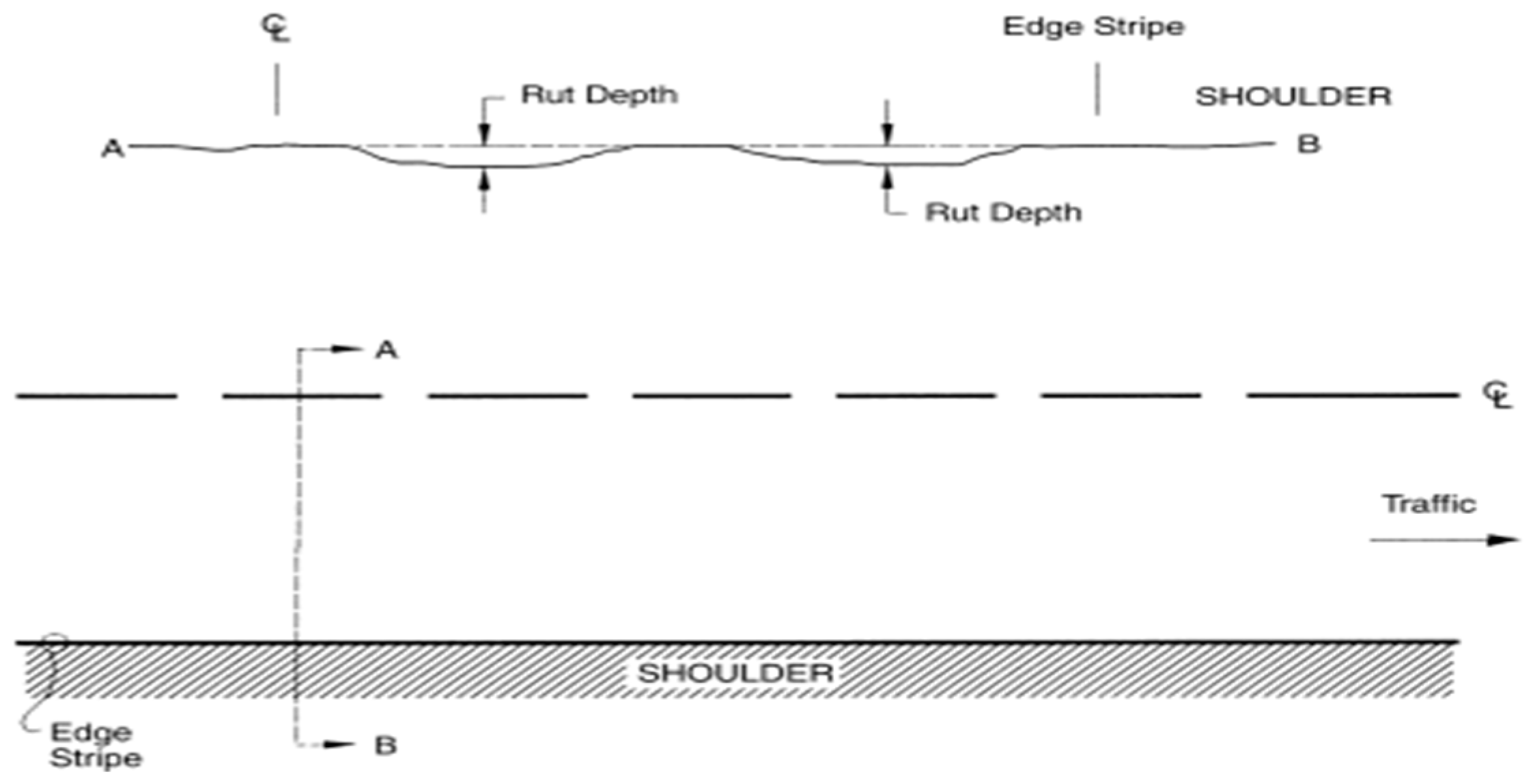
The ability to accurately predict its development is important not only for an effective pavement management system but also for the mechanistic-empirical pavement design technique for the examination of pavement structure and materials. A change in cross profile impacts driving safety, reduces skid resistance, and increases pavement damage (dynamic loading, narrow wheel loading distribution, etc.), as is shown in Figure 1 below, which displays a cross-section of a road and how the rut depth looks. The production of continuous deformation in asphalt layers is usually defined as a two-stage process. The first stage mostly comprises consolidation (densification with volume change), while the second stage primarily consists of shear deformation (plastic flow not associated with volume change). Consolidation and shear deformation can happen at the same time in extreme situations, causing severe layer distortion.
The Long-Term Pavement Performance (LTPP) initiative, which began in 1987 as a part of the Strategic Highway Research Program (SHRP) and has been managed by the Federal Highway Administration (FHWA) since 1992, analyzes the performance of in-service pavements. The LTPP program’s main purpose is to figure out how and why pavements behave the way they do. LTPP has provided several advantages in terms of field data collection equipment and techniques. Ninety percent of state transportation agencies, according to estimates, use LTPP data collection equipment or test procedures. The American Association of State Highway and Transportation Officials (AASHTO) and the industry have established several LTPP data collection methodologies. The goal of the LTPP initiative was to collect data that would be useful in describing elements that affect pavement performance. Consistency and accuracy in data gathering are critical from site to site as well as across States and Provinces. It is populated with the finest quality data available thanks to extensive quality assurance methods.
An Artificial Neural Network (ANN) is a system that functions similarly to a fully formed human brain, storing and retrieving data to solve complicated problems and gain knowledge through experience. An ANN is a collection of connected units (nodes), which are called artificial neurons. These units resemble the original neurons of a human brain. A set of inputs, weights, and a bias value are used to construct each node. The hidden layers contain the neural network weights. Weights and biases are machine learning parameters that are changed during neural network training. It generates its own rules from the learned examples to solve complex problems [6].
2. Literature Review
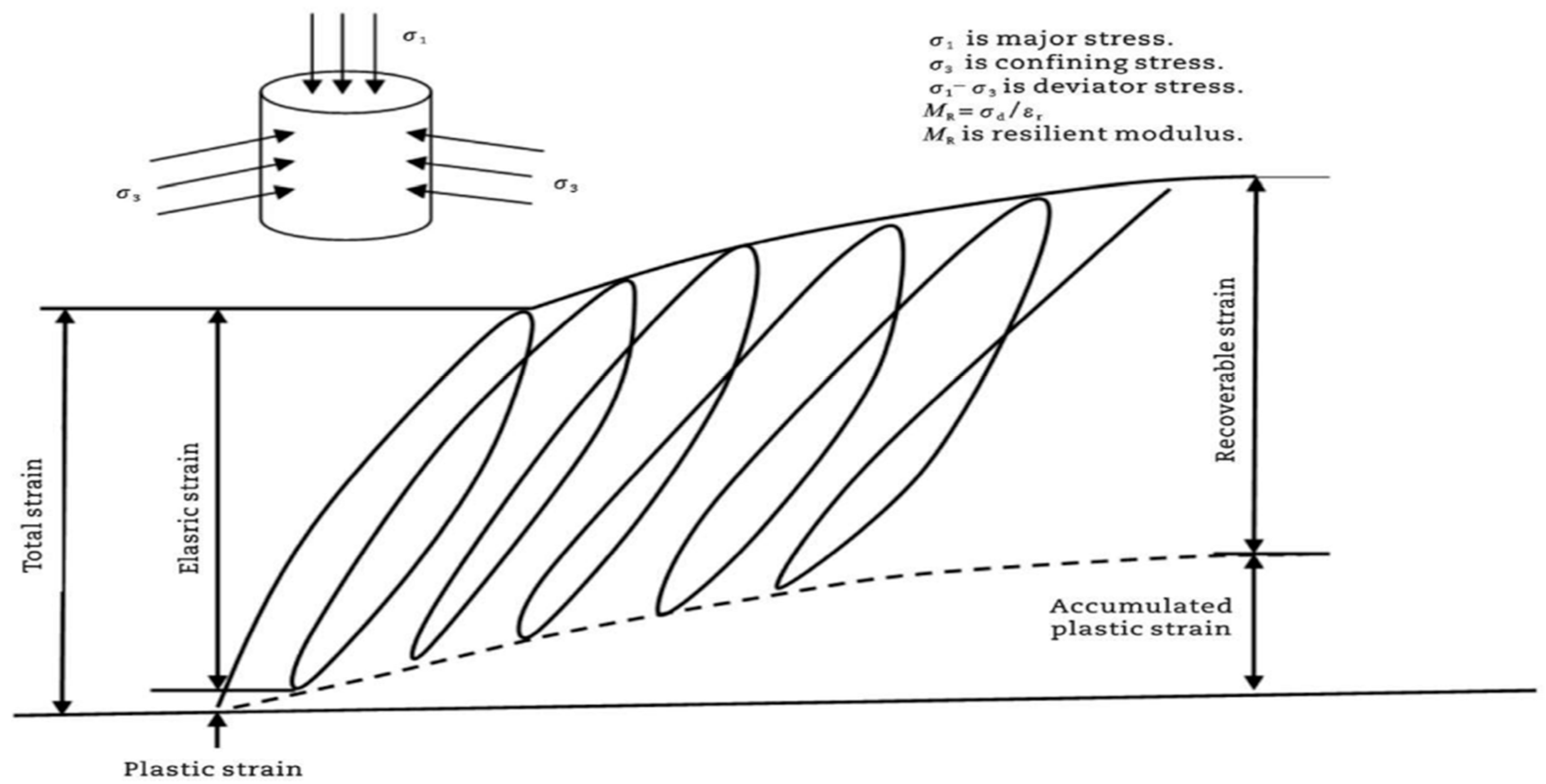
Rutting is one of the most common types of pavement distresses in flexible pavements, and it occurs because of frequent traffic loading movement. There are two types of deformation in the pavement layer: recoverable deformation (resilient behavior) and non-recoverable deformation (absorbing behavior). Resilient behavior is mostly used for current design practices, and Figure 2 below shows the difference between the elastic strain and plastic strain for the soil’s behavior [1].
Gradation, asphalt and moisture contents, type of aggregate, density, compaction method, temperature, amplitude and frequency of loading, and duration of each load cycle can all affect the behavior of asphalt-bound layers, unbound aggregate bases, and foundation soils (subgrades). Ruts are formed because of accumulated deformations caused by traffic distribution. The behavior of the materials should be known to be calculated or predicted for design purposes. Traffic and temperature were used as inputs to develop a model in PAVRUT by assuming the volume and characteristics of the traffic stream and the properties of the paving materials [8]. In addition, rutting causes the road surface to become uneven, spotty, and rough, affecting vehicle handling and perhaps creating a safety risk. Pavement design requires the capacity to estimate the amount and growth of the rutting in flexible pavements. A time-dependent ANN-based rut depth prediction model was constructed by [9].
The Asphalt Rubber Hot Mix-Gap Graded (ARHM-GG) overlays appear to give less protection against rutting to the underlying layers at increased temperatures than the DGAC overlays. Because of the DGAC overlays’ greater thickness and stiffness, they also suggested that Caltrans should also monitor tire pressure and loads on the truck fleet. They found that an increase in tire pressure will increase the probability of rutting [10]. They use a model to observe the macro behavior of mixes subjected to shear strain, an increase in shear modulus under the influence of hydrostatic pressure caused by heavy traffic, and variation in behavior due to changes in temperature and type of loading and accumulation of permanent deformation under repetitive loading to predict rutting [11].
The shear property of structure and materials, as well as traffic and environmental characteristics, are used to create a shear-based rutting prediction model. Full-scale pavement testing and laboratory wheel tests at varying temperatures, pressures, and slab thicknesses were used to obtain the parameters of the prediction model [12]. The structural responses (stress–strain deflection) are linked to Asphalt Cement (AC) fatigue cracking and rutting in component pavement layers (AC surface, granular base, subbase layers, and subgrade) [1]. Temperature and Stress levels are essential to determine permanent deformation. The authors in [13,14] stated that the slopes of the plot between permanent strain and stress repetitions will be unaffected.
Using an IC section, the foundation type, lane type, surface type, and accumulated number of vehicles were used as inputs to develop a prediction model of rutting depth; the authors in [15] stated that this study was limited to the Hokuriku expressway. The authors in [16] studied the effects of temperature and traffic using the ABAQUS finite element program, and found that the significant effects of both thermal and traffic loading conditions on the rutting damage of flexible pavement, and higher temperatures will provide a high rut depth more than traffic loading for the asphalt layer, base layer, and subgrade layer. Local empirical models were used by the authors in [17] to calculate permanent deformation such as environmental and traffic conditions using ANSYS software. They considered Equivalent Single Axle Load (ESAL) and wheel spacing with tire contact pressure and assumed homogeneous and isotropic materials with a specified resilient modulus and Poisson’s ratio. A previous study predicted the rut depth by ANN using viscoelastic parameters by trying to provide a model that can estimate the rutting depth; the model provided good accuracy with a high R-value [18]. The neural network model for rutting depth agreed well with the experimental data. Given the high R values, it is possible to conclude that the neural network model can predict rut depth with an acceptable level of accuracy [19].
3. Objectives
- To develop a prediction model using ANN to predict rutting depth.
- To extract an equation from ANN using weights and biases from ANN output.
- To perform a sensitivity analysis of the ANN model.
4. Data Collection
In this study, the data were collected from the LTPP database for the state of Texas. A total of 70 observations from 5 sections were extracted from LTPP based on the availability of data. Data for four input variables Temperature, Thickness, ESAL, Resilient Modulus, and one output Rutting depth were obtained to predict the rutting depth.
5. Data Selection
Based on the literature review, it was shown that the environmental changes, the thickness of the asphalt layer, the resilient modulus of the soil underneath the asphalt layers, and the frequency of the repeated load. Based on that, it can be concluded the four input variables (Temperature, Thickness, Resilient Modulus, and ESAL) were extracted from the LTPP database to build an ANN model to predict rutting depth. Regression analysis was performed between the variable inputs and outputs to find the correlation. An R2 value of 0.6444 was obtained, which means that the 64.4% of the output values are explained by the input variables. The difference between R2 and adjusted R2 is very small, adding another reason to use other ways of regression to predict the model and to significantly increase prediction accuracy (Table 1).
The results from the regression analysis are good to proceed to develop a prediction model for rutting depth to enhance the R2 to obtain better results. Table 2 shows the hypothesis testing values for input variables.
6. Developing a Prediction Model Using ANN
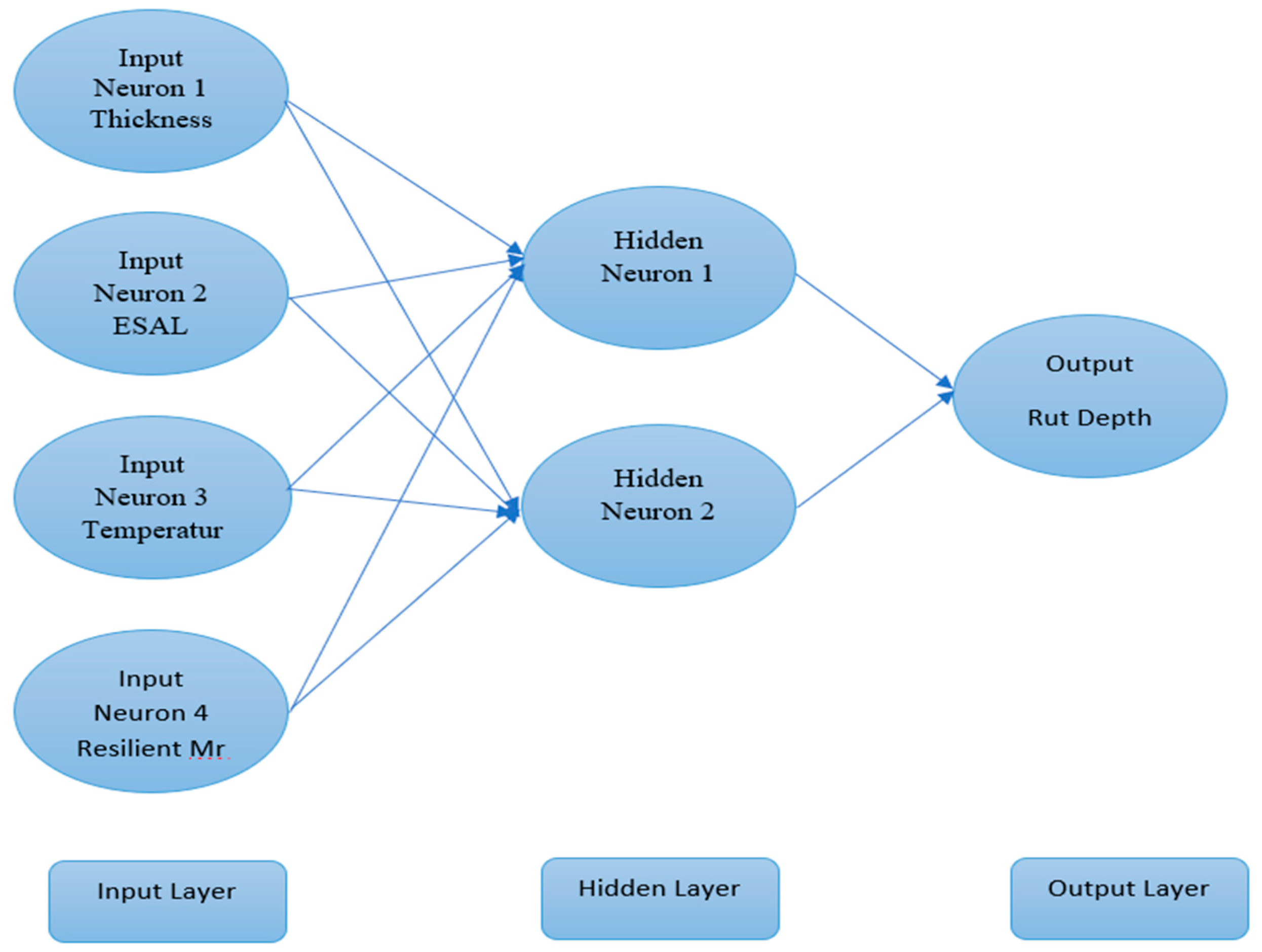
One recent advancement in deep learning is ANN. A computational model called ANN imitates how neurons work in the human brain. Simply said, ANN uses learning algorithms that can be modified by themselves as they gather new data. Therefore, they provide a great modeling tool for non-linear statistical data. ANN models typically consist of three layers linked by weighted linkages. The input layer is the top layer, directly connected to the hidden layer, while the output layer is the third layer [20,21]. A prediction model for Rutting Depth is developed using 4 input variables and 70 observations (Figure 3). The main aim was to develop an ANN-based prediction model with fewer hidden neurons possible to obtain the best results and to extract an equation. A multilinear ANN was used to predict, with four hidden neurons to obtain a simplified equation with a good R2 value.
The architecture of the constructed ANN model includes an input layer that has four input variables (neurons), which were initially normalized, and the second layer (hidden layer) has four hidden neurons that receive the result of matrix multiplication and addition, and at the end, there is an output layer consisting of a single output neuron with the value of the predicted rutting depth. The weights and biases of the hidden layer are represented by Wih and Bih. The input in the hidden layer is converted to a hyperbolic tangent using the hyperbolic tangent function. The output from the hyperbolic tangent is used to multiply with output weight and bias from the hidden layer. In the end, the normalized output obtained from the output layer is then denormalized to obtain our desired output. It can be understood using a flow chart as shown in the figure below [22]. The model was developed and trained using MATLAB (MATLAB, 2020A).
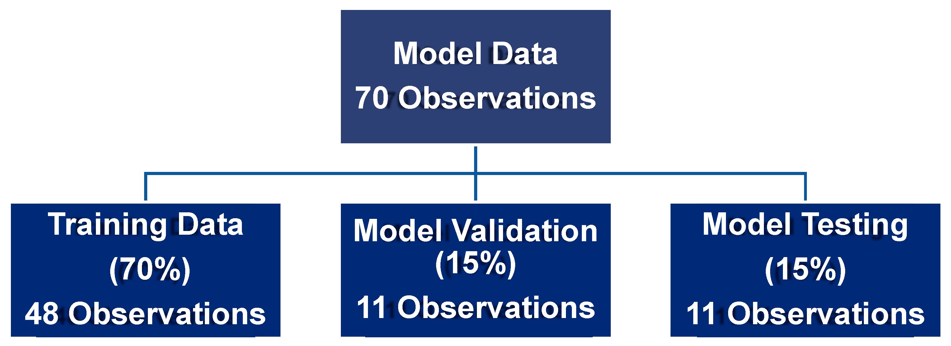
ANN model is trained to give desired R2 value; in which, out of 70 observations, 70 percent of the randomly selected data is used for training, 15 percent of the data is used for model validation, and the remaining 15 percent of the data is used to test the model (Figure 4). To prevent the model from overfitting, the input data were divided into three categories. Otherwise, the model would remember each data point from the training and perform poorly in a fresh database.
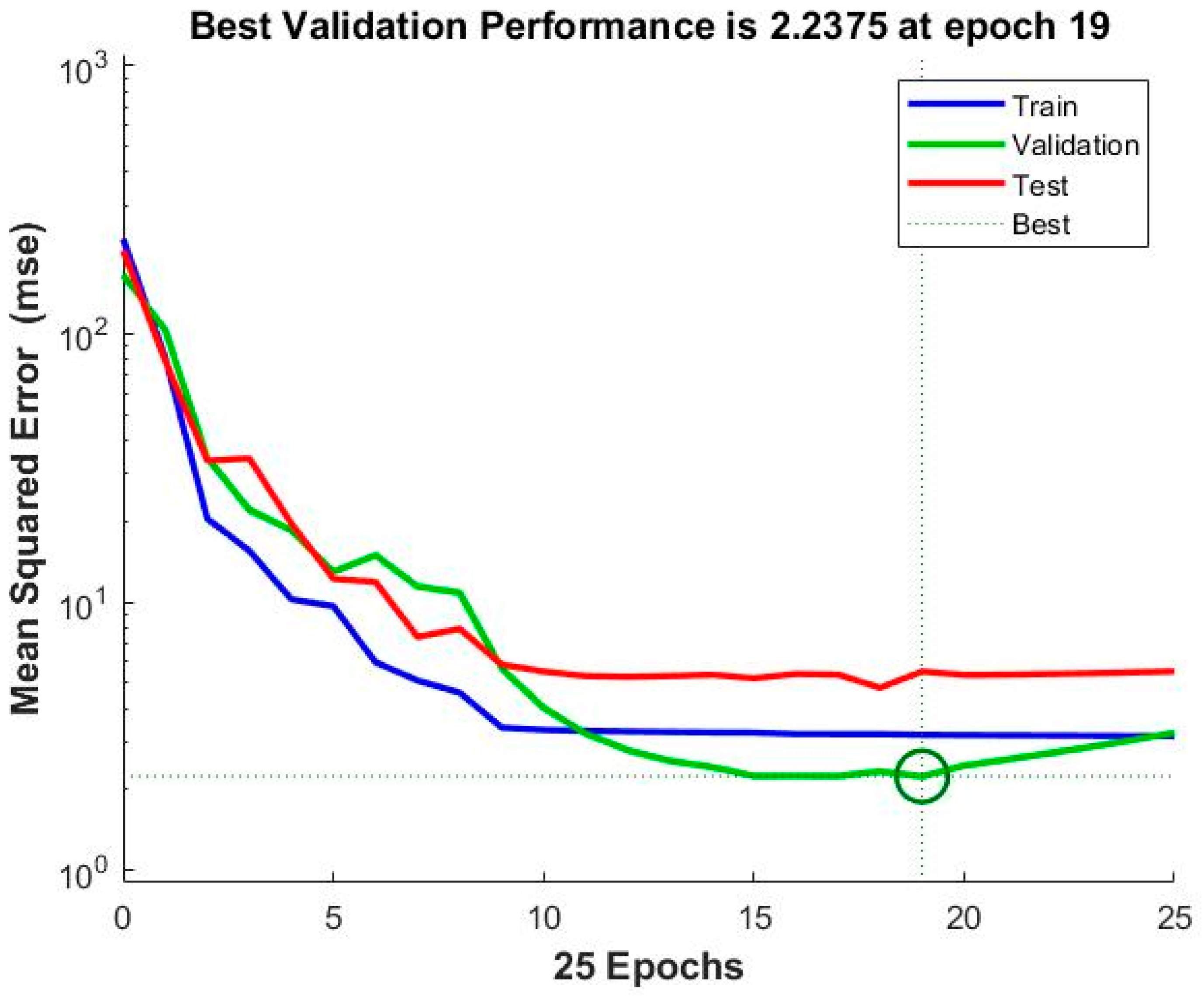
Every input was normalized between [−1, 1] to reduce the influence of variables with a huge numerical value. The normalized output is then finally denormalized to obtain the actual output value. The ANN algorithm allocates weights and biases at random in the first iteration. Then, the model’s output is compared to the training observations measured data. The error is the difference between the ANN model output and the measured output. The goal of the training was to reduce the Mean Square Error (MSE) as much as possible by altering the weights and biases with each iteration. Backpropagation was used to modify the weights and biases. An epoch is a unit of time that includes both forward and backward propagation. With each epoch, the model’s MSE is improved. Figure 5 shows that the best performance of the model was at the 19th iteration with 2.2375 MSE.
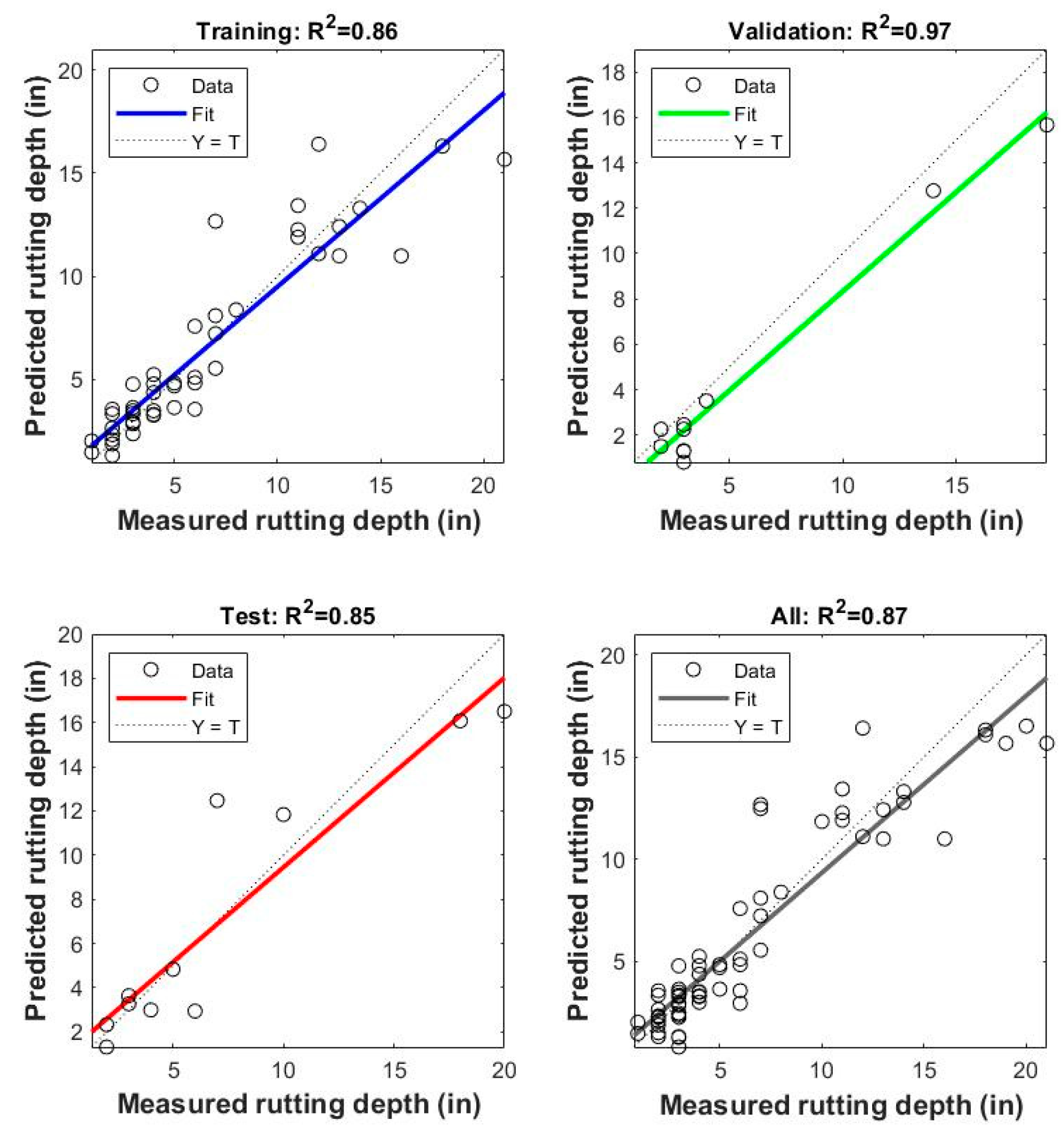
Every step of the model’s performance was evaluated using linear regression. The regression graphs from the training, validation, and testing phases are shown in Figure 6. The perfect model is shown by the 45-degree line of equality, in which the output and target value are the same. Here, the model has an overall R2 of 0.87 in the regression plot, which gives a high correlation coefficient and positive linear relation.
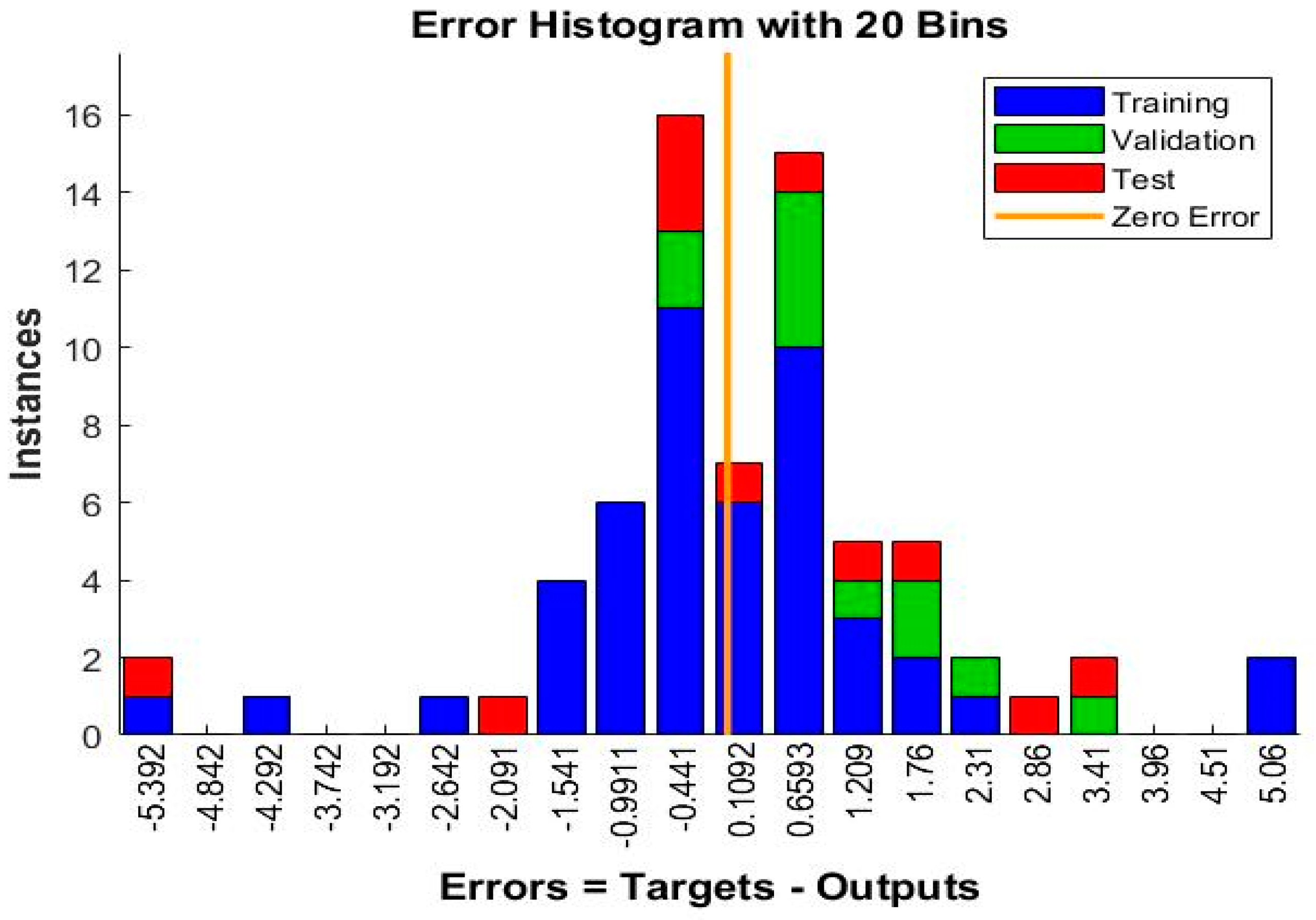
The histogram of errors between target values and predicted values after training a feedforward neural network is known as the error histogram. These error numbers can be negative because they represent how anticipated values depart from target values. The number of vertical bars shown below in Figure 7 is considered bins. The number of samples from the dataset that fall into each category is represented on the Y-axis.
7. Extraction of Weights and Biases from the ANN Model
Because of its versatility, the repeatable predictive model is very popular. As the activation function, the tangent hyperbolic function is employed. By using weights and biases from ANN a rutting depth equation can be obtained by using the below equation form.
where
Rutting Depth = d ({Woh × Tanh (Wih × In + Bih)} + Boh)
d = denormalization operator.
Wih =Weights from Input (First Hidden Layer).
Bih = Input Biases.
In = Normalized Input variables.
Who = Weights from hidden layer to output.
Boh = Biases from hidden layer to output.
The normalized Equation is given by
where
Xmin = Minimum value of the variable x.
Xmax = Maximum Value of the variable x.
The Weights and Biases obtained from ANN’s output after Training, Testing, and Validation are shown in the form of a matrix below.
The model’s weights and biases are used to derive an equation. The extracted equation is written below.
where
D = 10 × (0.7805 × TANH (1.234 × H − 8.56 × 10⁻⁷ × ESAL + 0.473 × T + 0.662 × MR − 31.52) +0.208 × TANH (0.308 × H − 2.209 × 10⁻⁶ × ESAL − 0.477 × T + 1.17 × MR − 10.26) +1.05 × TANH (−0.22 × H − 1.47 × 10⁻⁶ × ESAL + 0.319 × T − 0.658 × MR + 3.53) + 2.315 × TANH (0.64 × H + 4.83 × 10⁻⁷ × ESAL − 0.06 × T + 0.836 × MR − 12.26) − 1.385 + 1) +1
D = Rutting Depth (in).
H = Thickness (in).
ESAL = Equivalent Single Axle Load.
T = Temperature (C°).
MR = Resilient Modulus (ksi).
8. Sensitivity Analysis
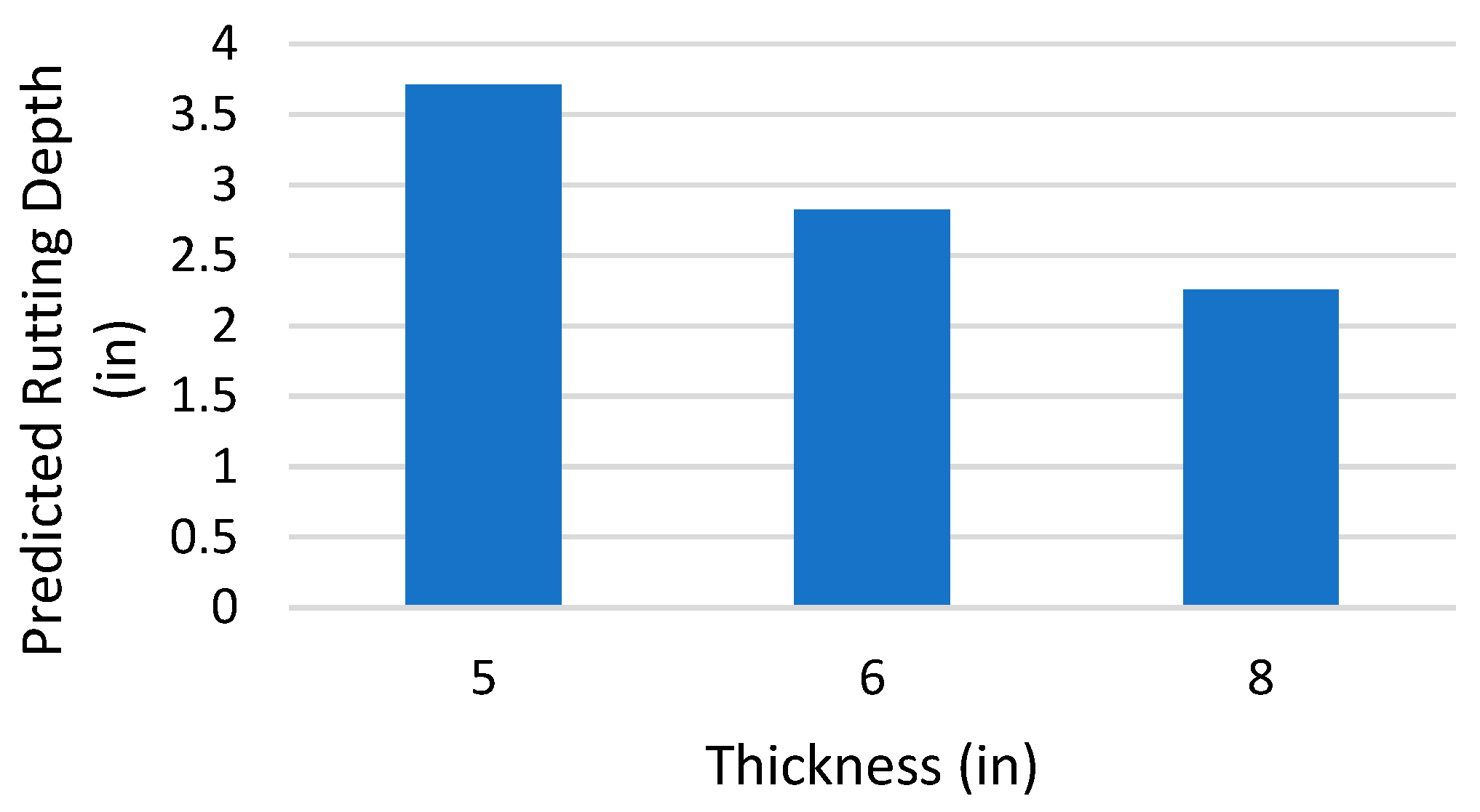
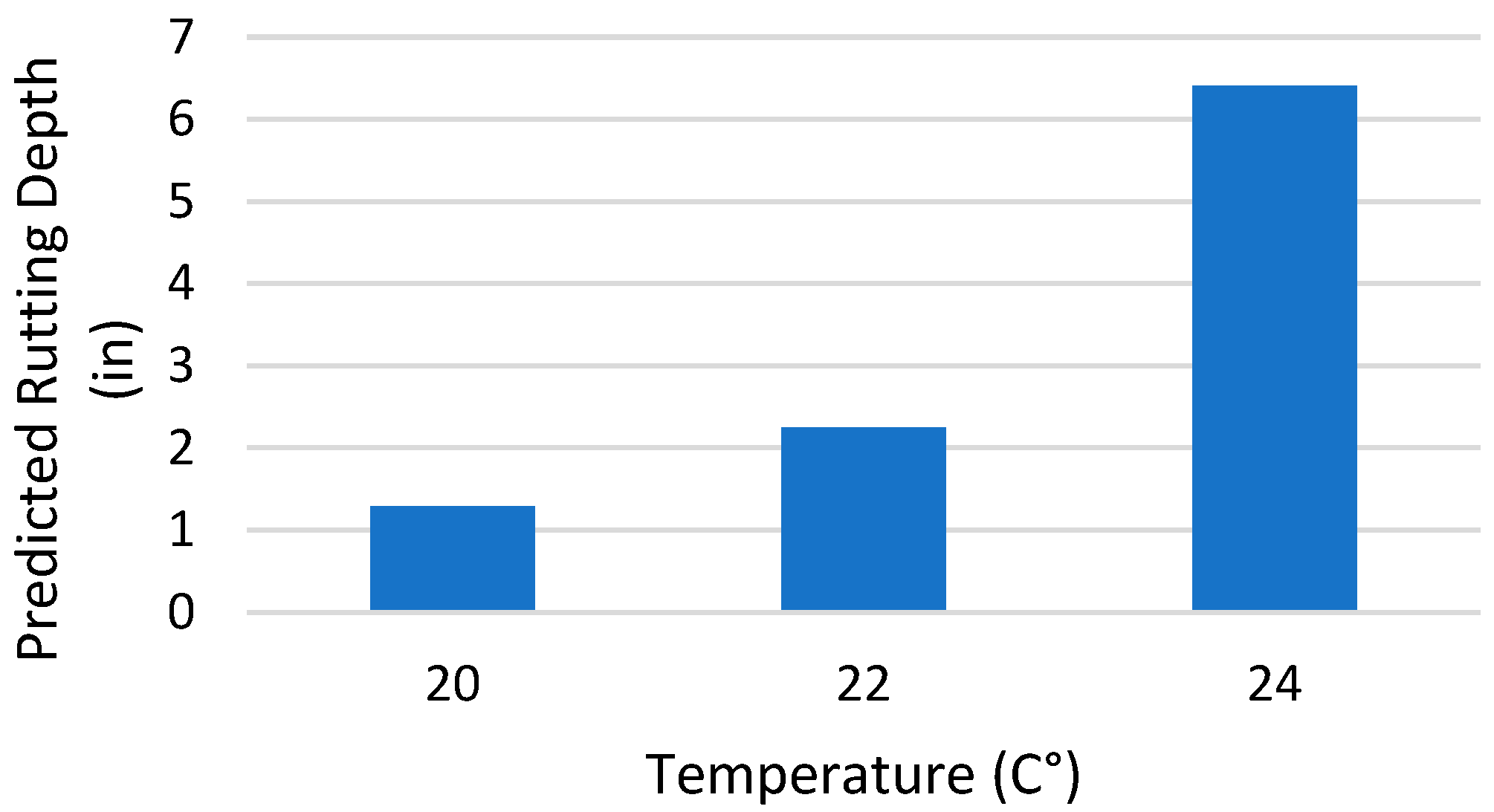
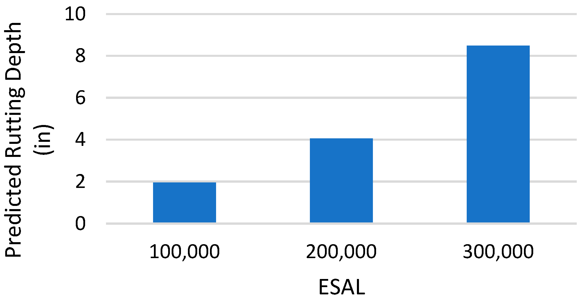
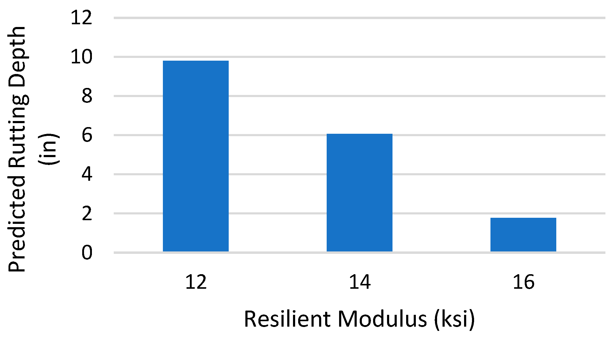
One of each input variable is chosen for sensitivity analysis, while the remaining variables are retained at their average value. The output of the model is recorded as the selected variable changes and the values recorded and the same are plotted on a bar chart. For sensitivity analysis, the anticipated Rutting Depth vs. the single input variable bar chart is displayed using those data. Table 3 contains the minimum, maximum, and average values for all variables in this procedure. Figure 8, Figure 9, Figure 10 and Figure 11 below show how the change in each input can affect the rutting depth.
The results of the sensitivity analysis for rutting depth showed that input variables such as temperature and ESAL are directly correlated with the dependent variable, the rutting depth. Whereas, thickness and the resilient modulus were inversely correlated to the rutting depth.
9. Summary and Conclusions
A rutting depth prediction model was developed using ANN. Seventy observations extracted from the LTPP database were used for the data collection, the model was fed with four inputs; temperature, ESAL, resilient modulus, and thickness. an R2 with a value of 0.87 was developed. Comparing this R2 with the 0.64 that was observed from the linear regression, the ANN shows a better result and higher R2. An Equation was extracted using weights and biases and verified for rutting depth. The extracted equation and ANN output were checked using a regression plot, and the R2 value of 1 was obtained. The output of the extracted equation is identical to that of the model. To achieve the desired performance, the significant factors found in the sensitivity analysis might be tweaked. The sensitivity analysis showed that the temperature and ESAL affect the rutting depth very strongly in a direct way. Moreover, thickness and resilient modulus affect the model but in an indirect relation. The final output may be used for pavement performance prediction and modeling.
Author Contributions
The authors confirm contribution to the paper as follows: Conceptualization, R.K., M.I.S. and M.B.M.B.; methodology: R.K., M.I.S. and M.B.M.B.; software: R.K. and M.B.M.B.; validation: R.K., M.I.S. and M.B.M.B.; formal analysis: R.K., M.I.S. and M.B.M.B.; investigation: R.K., M.I.S. and M.B.M.B.; data curation: M.I.S. and M.B.M.B.; writing—original draft preparation: M.I.S. and M.B.M.B.; writing—review and editing: R.K. and M.I.S.; visualization: R.K. and M.I.S.; supervision: M.I.S. All authors have read and agreed to the published version of the manuscript.
Funding
This research received no external funding.
Data Availability Statement
Data available upon request.
Conflicts of Interest
The authors declare no conflict of interest.
References
- Tayfur, S.; Ozen, H.; Aksoy, A. Investigation of rutting performance of asphalt mixtures containing polymer modifiers. Constr. Build. Mater. 2007, 21, 328–337. [Google Scholar] [CrossRef]
- Archilla, A.R.; Madanat, S. Development of a pavement rutting model from experimental data. J. Transp. Eng. 2000, 126, 291–299. [Google Scholar] [CrossRef]
- Wang, H.; Zhang, Q.; Tan, J. Investigation of layer contributions to asphalt pavement rutting. J. Mater. Civ. Eng. 2009, 21, 181–185. [Google Scholar] [CrossRef]
- Singh, A.K.; Sahoo, J.P. Rutting prediction models for flexible pavement structures: A review of historical and recent developments. J. Traffic Transp. Eng. (Engl. Ed.) 2021, 8, 315–338. [Google Scholar] [CrossRef]
- Banik, B.K.; Chowdhury, M.A.I.; Hossain, E.; Mojumdar, B. Road accident and safety study in Sylhet Region of Bangladesh. J. Eng. Sci. Technol. 2011, 6, 493–505. [Google Scholar]
- Zell, A. Simulation Neuronaler Netze (Simulation with Neuronal Networks); Wissenschaftsverlag: Oldenbourg, Germany, 2003. [Google Scholar]
- Huang, Y.H. Pavement Analysis and Design; Pearson Prentice Hall: Upper Saddle River, NJ, USA, 2004; Volume 2, pp. 401–409. [Google Scholar]
- Allen, D.L.; Deen, R.C. A computerized analysis of rutting behavior of flexible pavement. Transp. Res. Rec. 1986, 1095, 1–10. [Google Scholar]
- Abiola, O.S.; Owolabi, A.O.; Sadiq, O.M.; Aiyedun, P.O. Application of dynamic artificial neural network for modelling ruts depth for lagos-ibadan expressway, Nigeria. ARPN J. Eng. Appl. Sci. 2012, 7, 987–991. [Google Scholar]
- Harvey, J.; Popescu, L. Rutting of Caltrans Asphalt Concrete and Asphalt-Rubber Hot Mix Under Different Wheels, Tires and Temperatures–Accelerated Pavement Testing Evaluation; University of California: Berkeley, CA, USA, 2000. [Google Scholar]
- Sousa, J.; Weissman, S.L.; Sackman, J.L.; Monismith, C.L. Nonlinear Elastic Viscous with Damage Model to Predict Permanent Deformation of Asphalt Concrete Mixes; Transportation Research Board: Washington, DC, USA, 1993. [Google Scholar]
- Sun, L.; Su, K.; Liu, L.P.; Tang, W.; Lu, Z.L. Development of shear-based rutting prediction model for asphalt pavements. In Proceedings of the 11th International Conference on Asphalt Pavements, Nagoya, Japan, 1–6 August 2010; pp. 1–6. [Google Scholar]
- Thompson, M.R.; Nauman, D. Rutting Rate Analyses of the AASHO Road Test Flexible Pavements; Transportation Research Board: Washington, DC, USA, 1993. [Google Scholar]
- Allen, D.L.; Deen, R.C. Rutting Models for Asphaltic Concrete and Dense-Graded Aggregate from Repeated-Load Tests; Annual Meeting of The Association of Asphalt Paving Technologists: Louisville, KY, USA, 1980. [Google Scholar]
- Shigehara, D.; Nishizawa, T.; Komatsubara, A.; Nakagen, T. A Model of Rutting Development of Asphalt Pavement in Expressway Based on Artificial Neural Network. In Proceedings of the 11th International Conference on Asphalt Pavements, Nagoya, Aichi, Japan, 1–6 August 2010. [Google Scholar]
- Alkaissi, Z.A. Effect of high temperature and traffic loading on rutting performance of flexible pavement. J. King Saud Univ. Eng. Sci. 2020, 32, 1–4. [Google Scholar] [CrossRef]
- Abed, A.H.; Al-Azzawi, A.A. Evaluation of rutting depth in flexible pavements by using finite element analysis and local empirical model. Am. J. Eng. Appl. Sci. 2012, 5, 163–169. [Google Scholar]
- Kamboozia, N.; Ziari, H.; Behbahani, H. Artificial neural networks approach to predicting rut depth of asphalt concrete by using of visco-elastic parameters. Constr. Build. Mater. 2018, 158, 873–882. [Google Scholar] [CrossRef]
- Mirabdolazimi, S.M.; Shafabakhsh, G. Rutting depth prediction of hot mix asphalts modified with forta fiber using artificial neural networks and genetic programming technique. Constr. Build. Mater. 2017, 148, 666–674. [Google Scholar] [CrossRef]
- Saha, S.; Gu, F.; Luo, X.; Lytton, R.L. Use of an Artificial Neural Network Approach for the Prediction of Resilient Modulus for Unbound Granular Material. Transp. Res. Rec. 2018, 2672, 23–33. [Google Scholar] [CrossRef]
- Kim, S.H.; Yang, J.; Jeong, J.H. Prediction of Subgrade Resilient Modulus Using Artificial Neural Network. KSCE J. Civ. Eng. 2014, 18, 1372–1379. [Google Scholar] [CrossRef]
- Acharjee, P.K.; Souliman, M. Development of Dynamic Modulus Predictive Model Using Artificial Neural Network (ANN). In Proceedings of the 2022 ASEE Gulf Southwest Annual Conference, Prairie View, TX, USA, 16–18 March 2022. [Google Scholar]
Figure 1.
Top view and Cross-Sectional View of Rutting depth.

Figure 2.
Definition of recoverable strain and soil resilient modulus [7].
Figure 2.
Definition of recoverable strain and soil resilient modulus [7].

Figure 3.
The architecture of the developed ANN Model.

Figure 4.
Flow Chart for use of data for Training, Validation, and Testing.

Figure 5.
The Mean Square Error in 25 Epochs.

Figure 6.
Regression Plot from ANN output.

Figure 7.
Error Histogram obtained from ANN.

Figure 8.
Model sensitivity for Thickness.

Figure 9.
Model sensitivity for Temperature.

Figure 10.
Model Sensitivity for ESAL.

Figure 11.
Model Sensitivity for Resilient Modulus.


Table 1.
Regression statistics for input variable to predict Rutting.
| Regression Statistics | |
|---|---|
| Multiple R | 0.80 |
| R2 | 0.64 |
| Adjusted R2 | 0.62 |
| Standard Error | 3.16 |
| Observations | 70 |
Table 2.
Hypothesis testing values for input variables.
| Coefficients | Standard Error | t Stat | p-Value | |
|---|---|---|---|---|
| Intercept | −52.51 | 7.26 | −7.23 | 6.72 × 10⁻¹⁰ |
| Thickness | 2.10 | 0.26 | 7.90 | 4.45 × 10⁻¹¹ |
| ESAL | −1.55 × 10⁻⁵ | 3.65 × 10⁻⁶ | −4.25 | 6.95 × 10⁻⁵ |
| Temperature | 2.70 | 0.26 | 10.41 | 1.76 × 10⁻¹⁵ |
| Resilient Modulus | −0.76 | 0.25 | −2.97 | 4.18 × 10−0.3 |
Table 3.
Maximum, Minimum, and Average values for all input and output variables.
| Thickness (in) | ESAL | Temperature (°C) | Resilient Modulus (ksi) | Rut Depth (in) | |
|---|---|---|---|---|---|
| Average | 6.59 | 218,056.5 | 22.08 | 14.93 | 6.32 |
| Std Deviation | 2.37 | 161,725.88 | 3.09 | 1.61 | 5.15 |
| Min | 2.99 | 3011 | 16.20 | 13.35 | 1 |
| Max | 10.90 | 557,000 | 25.5 | 17.77 | 21 |
Disclaimer/Publisher’s Note: The statements, opinions and data contained in all publications are solely those of the individual author(s) and contributor(s) and not of MDPI and/or the editor(s). MDPI and/or the editor(s) disclaim responsibility for any injury to people or property resulting from any ideas, methods, instructions or products referred to in the content. |
© 2023 by the authors. Licensee MDPI, Basel, Switzerland. This article is an open access article distributed under the terms and conditions of the Creative Commons Attribution (CC BY) license (https://creativecommons.org/licenses/by/4.0/).
Share and Cite
MDPI and ACS Style
Khalifah, R.; Souliman, M.I.; Bajusair, M.B.M. Development of Prediction Model for Rutting Depth Using Artificial Neural Network. CivilEng 2023, 4, 174-184. https://doi.org/10.3390/civileng4010011
AMA Style
Khalifah R, Souliman MI, Bajusair MBM. Development of Prediction Model for Rutting Depth Using Artificial Neural Network. CivilEng. 2023; 4(1):174-184. https://doi.org/10.3390/civileng4010011
Chicago/Turabian StyleKhalifah, Rami, Mena I. Souliman, and Mawiya Bin Mukarram Bajusair. 2023. "Development of Prediction Model for Rutting Depth Using Artificial Neural Network" CivilEng 4, no. 1: 174-184. https://doi.org/10.3390/civileng4010011