1. Introduction
The formulation of society was dependent upon the development of infrastructures, which made the environment friendly to humans [
1,
2,
3,
4,
5] and allowed them to live in groups (clusters), a condition that was proven necessary for growth and progress [
6,
7]. In order to support the fundamentals of prosperity (water-energy-food nexus [
8,
9]), humans constructed large infrastructure projects in order to minimize the cost of the unit. In theory, scale-economies were formulated by Adam Smith [
10,
11] in the late 18th century, while the division of labour [
12,
13] and dynamics of scale-economies was a crucial issue for infrastructure creation [
14,
15].
In prehistory and before the invention of money, the responsibility for the management of big infrastructures was laid on the elite, which was responsible for social stability and the distribution of wealth [
16,
17]. However, we cannot be certain about the rules and how the elite (for example, the elite of Minoans) performed the management for these constructions [
18], and how they distributed the wealth to society without the exchange of money and taxes [
19].
In our study, we try to show that it is erroneous to consider a stable interest rate (IR) in order to forecast the risk of an investment, since a variability of the IR is expected. Stochastic calculus has been helpful to quantify a wide range of heterogenous issues (e.g., economy, biology, acoustics, neurophysiology, telecommunications, aesthetics, art paintings, and more) [
20,
21,
22,
23,
24,
25,
26]. Therefore, using stochastic tools, we can simulate IR with synthetic timeseries estimating the risk of the investment.
The paper outline goes as follows: In
Section 2, we conduct the literature review. In
Section 3, we describe the methodology we followed, and we show the equations to estimate the cost of a unit. In
Section 4, we show the historical and stochastic approach of how to generate timeseries of IR by using an autoregressive AR(1) model. In
Section 5, we examine the case study of the water supply system in West Mani, we analyze the cost of the investment of the water infrastructure for three different solutions of the scale of capital investment, and we evaluate the risk in Greece, whereas in
Section 6, we evaluate the risk of the same investment in other countries. In
Section 7, we discuss the results of our study and broaden the discussion in the context of wartime financial instability. In
Section 8, we outline the conclusions of this research.
2. Literature review
Even if we assume that money is a stable measure that could help the sustainable management of big infrastructures, money has been formulated diachronically by its own rules that contain extreme variability (e.g., the value of denarius in the Second Century [
27,
28]).
IR (e.g., see definition in [
29]), was the basic tool to attempt to stabilize the value of money in time. The IR was developed in the Renaissance supporting trading, but it had a wide application after the industrial revolution, when the circulation of money became more intensive. IR of the investment is “the amount a lender charges a borrower and is a percentage of the principal—the amount loaned” [
30]. Stable IRs, in general, promote social stability in various ways, including preventing intergenerational wealth inequality [
31] and price stability [
32].
The history of IR is connected with a wide range of variability/fluctuation [
33] that is more intense in the 20th century. As IRs have variations in time, which are determined by the Central Bank of each country (or decided by market mechanisms), the cost of money exchange and the risk of the investment cannot be stable. However, the majority of the studies assume a stable IR in order to estimate the risk of the investment; Ingersoll and Ross [
34,
35] presented the argument that IR volatility could be as important as the IR itself in investment decisions.
The first papers about IRs appear in the mid-19th century. However, systematic research on IR and the cost of capital began a century later.
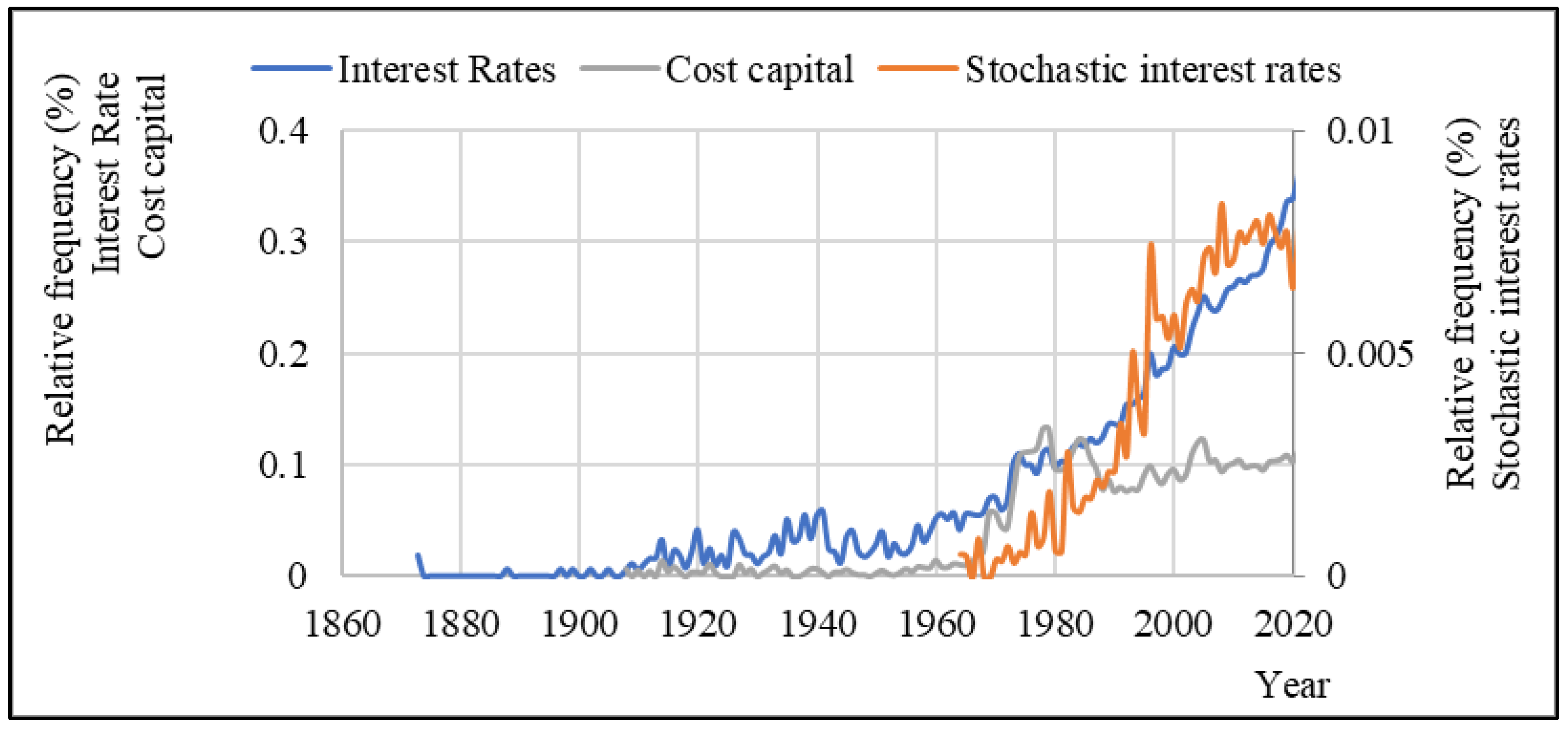
Figure 1 shows an increasing trend in the study of IR, the cost of capital, and the use of stochastics in the research of IR [
36,
37,
38,
39,
40,
41,
42,
43].
Regarding infrastructure projects, Tolis et al. [
44], have used IR and inflation rates as stochastic variables in an attempt to analyse energy investments. Other studies have used stochastic IR to calculate the cost of infrastructure [
45,
46,
47,
48,
49,
50].
It should be noted that no attempt has been made to compare different water supply infrastructures by using stochastic synthetic timeseries for the IR. In general, when decision-makers compare, for example, different options for water supply during the planning stages, many considerations and assumptions are made (environment, feasibility, adequacy, esthetics, etc.). Until now, all calculations are done without examining the capital structure of proposals and how that exposes the investment to macroeconomic factors. In this work, we attempt to make the first step to address this issue. Of course, risk is not expressed only through IRs, but as IRs are related to the cost of money, the IR is one of the most impactful factors for the long-term feasibility of an investment.
3. Methodology
Financial and investment studies contain abstract concepts, which are often confusing to non-insiders. Therefore, we are trying to simplify and visualize the concept of our methodology in order to be easily accessible to a wide audience.
Here, we consider the problem from the point of view of the investor (or bank), and in order to conceptualize the problem, we simulate it as a bathtub, as follows:
This bathtub is considered empty at first.
In the beginning, every year the bathtub is filled with more and more magic potion (capital), which must be available (investment on the project or borrowing) (
Figure 2a).
This magic potion is used to build infrastructures (capital cost) and fund the operations (operational cost).
Once the bathtub is filled, those infrastructures start bringing in income (revenue) and, consequently, the magic potion can be then withdrawn from the bathtub.
Therefore, the bathtub starts emptying (
Figure 2b).
However, this magic potion has a unique property: it expands (positive IR) for some years, while for some it diminishes (negative IR) (
Figure 2c).
In the end, we assume that after many years, there will be no more magic potion in the bathtub, which reflects the fact that the lifespan of the infrastructure has been depleted.
This somewhat childish analogy is nevertheless the basis to form an understanding of the problem.
An IR can be viewed as the percentage of an amount of money that is paid for its use over a period [
53]. In essence, the IR reflects the fact that the cost of the money varies [
54]. Usually, when studying the cost of infrastructure, one would use the methodology in which a single initial capital investment takes place, and over the years a stable amount is paid annually to cover the debt at a stable IR [
55].
The real IR (for a single year) is defined as the yield of the one-year treasury bond of a country minus the inflation rate for that year (Fisher equation) [
56]; however, this should not be confused with the cost of capital that expresses the rate available for borrowers by banking institutions [
57].
In our calculations, we use the real IR, , where all are assumed as stochastic variables. In order to estimate the total investment, we use the following equations.
The total expenditure during a given year is provided by the Equation (1):
where:
: Total expenditures during year
T;
: Amount of that was spent in the year
T for buying or building fixed assets;
: Amount that was spent to maintain operations in the year
T (note: because the assumption is that all infrastructure will operate at maximum capacity during the entire lifespan of the project, the operational cost is assumed constant and not a function of units produced or sold). The revenue during a given year is provided by Equation (2):
where:
: revenue during year
T;
: cost of unit;
: number of units produced, (note: during construction revenue is 0). A stochastic estimation of the present value of the expenditures of a given year T is provided by Equation (3), and the present value of all future expenditures is provided by Equation (4):
where:
: present value of all future expenditures for a period
T;
: Present value of a future expense in the year
T;
: IR for year
T.
The present value of all future expenditures, assuming that the IR is fixed, is described by Equation (5):
In the same manner, we replace expenses with revenue. Therefore, a stochastic estimation of the present value of the revenue of a given year
T is provided by Equation (6) and the present value of all future expenditures is provided by Equation (7):
For calculation purposes and during the years with no revenues, we consider revenues to be 0.
The present value of all future revenues, assuming that the IR is fixed, is described by Equation (8):
Using the above equations, we calculate the expenditures for a given year (Equation (1)). We then calculate the present value of expenditures for each given year (Equation (3)). Afterwards, we calculate the present value of expenses during the lifespan of the project (Equation (4)). Finally, we assume the present value of all expenses to be equal to the present value of all future revenue, repeating the process backwards (Equations (2), (6) and (7), and enabling us to calculate the unit cost in each case.
It is arguably unusual for the calculation of the cost of water to engage in such complicated modeling. Various common methodologies assume the IR to be fixed [
58], and a lot of research has been put into deciding the ‘correct’ stable IR [
59]. The fact that the IR is assumed as fixed, is not a simplification of calculations but rather a reflection of the way public infrastructures are financed, and comprised of stable financial vehicles such as bond issuance [
60]. Nevertheless, it is important, in our view, to study the IR as a variable function, since interest payments ultimately are not stable. The above can take many forms, including a change in expectations of investment returns or, in the case of governments, a change in economic conditions, which in turn may cause changes in the government’s budget [
61].
Multiple financial tools exist to take advantage of, or shield, an investment from that fact, such as issuing bonds of different durations. Furthermore, if the infrastructure project is partially or fully funded by private entities, then these funds would be considered as opportunity cost, which is simply the ability to invest in other more promising available investments [
62], when making investment decisions.
4. Modeling of Investments’ Risks
From the above, one may get the wrong impression that this work attempts to predict or forecast future IR values. Forecasting, in our view, is a fundamentally different process than stochastic modeling., and the main difference is ultimately a philosophical one. Modern-day forecasting was born out of Keynesian thought, and it ultimately attempted to predict the future behavior of the economy [
63]. This was necessary in order to conduct macroeconomic public policy; however, the first such attempt [
64] failed to predict the Great Recession. In subsequent years, despite ever-increasing computing power, economists have very poorly predicted in advance any major macroeconomic events. On the other hand, weather forecasting has become better at predicting tornadoes [
65].
The tradition of forecasting usually aims at producing a single prediction, but this impacts the operational principles of forecasting. Specifically, general principles on forecasting [
66] suggest: ‘Do not forecast cycles; Adjust for events expected in the future; Be conservative in situations of high uncertainty or instability’.
These previous principles stand against the tradition of hydrological engineering. The seasonality and unpredictability of hydrological phenomena, in no case, allows us to implement such methodologies, especially when these are what we seek to ‘design around’. Furthermore, we under no circumstances aim to make predictions. Our aim is to produce a range of outcomes along with the associated distribution function (i.e., Monte-Carlo approach), which we achieve by modeling the system of infrastructures with extremely large input timeseries. The type of simulation we use is a terminating simulation [
67], where
n number of simulations are conducted under the same stochastic properties. Additionally, the creation of a single prediction creates a burden in forecasting methods to ‘prove themselves’ in backtesting (post-facto errors) [
68,
69]. Such burden does not weigh on models that simulate water infrastructure operations (e.g., ‘A timeseries is a series of observations taken at different times and recorded with the time at which they were taken.’ [
70]).
Considering the above fact, we use sampling data (annual real IR) [
71], as well as models for timeseries in discrete time. To simulate the IR, we will create an ensemble of 200 synthetic timeseries. These timeseries are created with the Markov assumption that every precedent value depends on the previous value (short-time dependence [
72]), and is implemented based on the autoregressive model of first-order, AR(1) [
73]. The distribution function of
was assumed Gaussian with mean and standard deviation and lag one autocorrelation equal to their estimates for each country (see
Table 1). In general, existing processes like auto-regressive moving average (ARMA) and auto-regressive integrated moving average (ARIMA) models [
74], are mainly used for mid-range tasks of stationary and non-stationary simulations, but in our view, the AR(1) model is adequate for the task at hand, which is to investigate for the first time in literature, the stochastic behaviour of the IR.
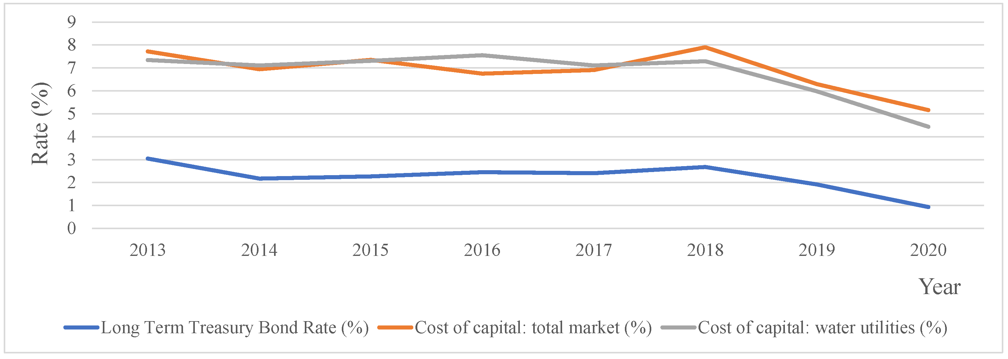
We note that by using the observed IR in our calculations, we essentially find the break-even cost and not the real cost of water. In order to find the real cost of water, one should use the cost of capital (WACC) as the discount rate. However, we choose to avoid using it, since (a) the cost of capital for governments is the long-term bond yields (i.e., the loans to countries that are considered as risk-free investments; blue line in
Figure 3), (b) WACC data are very scarce and not available in the requested high-quality, while data from 2013–2020 [
75], suggests that the average global WACC for the total market (grey line in
Figure 3) as well as WACC for the industry of water utilities, is approximately 4.5% more than the treasury yield (orange line in
Figure 3).
Nevertheless, data is very limited in range to draw conclusions in our view, and the research outcomes are not much affected, since we compare the results between solutions and countries using the WACC database.
Afterwards, we may use the synthetic timeseries of the IR, to estimate the final cost of money. As IRs are the primary measure of the cost of money, they will be the criterium in our evaluation. The first series of calculations will use the historical Greek IR. In the second series of calculations, we will use the historical IR from a basket of 18 selected countries, which reflect multiple development levels, considering that the world is generally divided into three wide areas (i.e., developed; developing; least developed) and each country may be treated differently, in the macroeconomic sense.
Stochastic evaluation of IRs could be a very important proxy of the investments’ risk, which is connected with the cost of money. In particular, no apparent pattern appears in the IR values, as presented in
Table 1 and shown in
Figure 4.
Another issue that is taken into consideration is that each technical solution needs a different level of capital intensity. The importance of the stochastic analysis of IR in order to estimate the risk of the investment is not related to technical scale, which is generally obedient in the accepted rules of econometry [
76]. Stochastic analysis of the IR mostly shows the fluctuation of the risk by the different scale of investment, rather than its physical footprint. Therefore, in this study, we highlight the cost of money by IR as the critical issue for the evaluation of the technical solution.
5. Case Study
5.1. General Description
The problem of the water supply system of West Mani has been analyzed in previous studies [
77,
78], whereas here, many different solutions, and in different scales, complexity, footprint, and approach, were considered. The diversity of the solutions, the intimate knowledge of the area, and, most of all, the complexity of the geography serve as an excellent case study to assess the investment risk of water infrastructures from the engineering viewpoint.
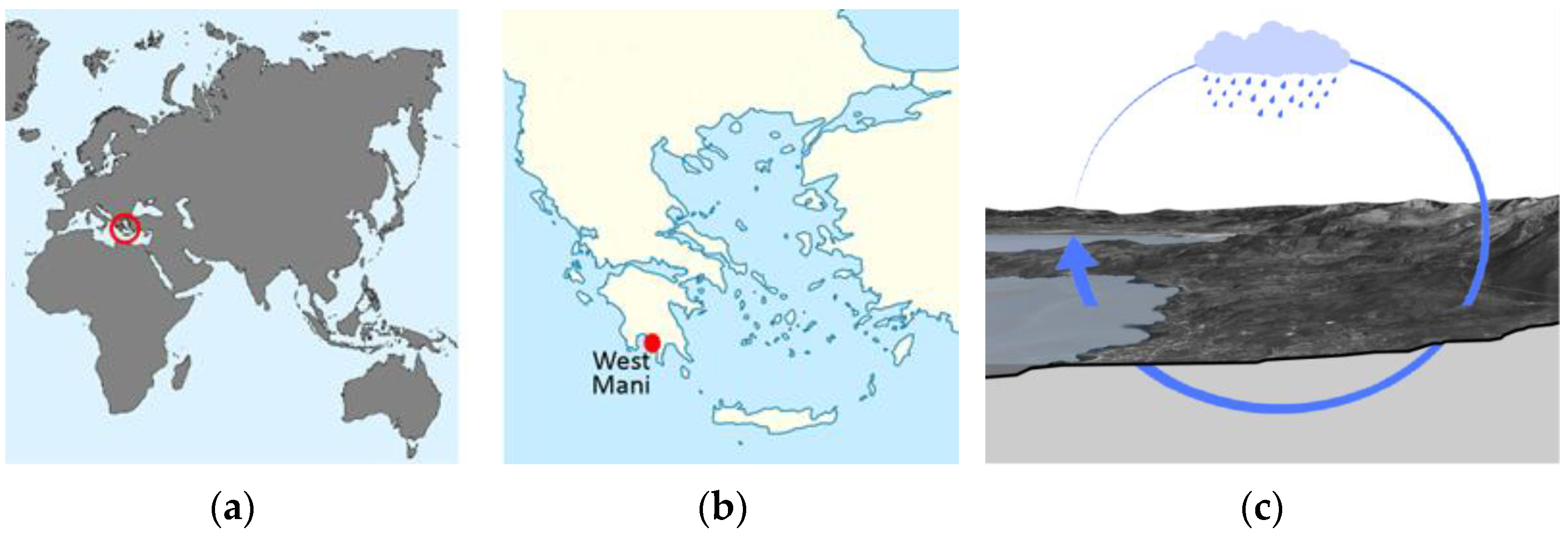
The area of West Mani is located in the southern part of Greece in the Peloponnese (
Figure 5a,b). The region has a high rate of precipitation, mainly in the mountainous areas. Rainfall is mostly observed during the autumn and winter months (i.e., from October to March), while there is a significant decrease in the summer.
The geological background is extremely permeable (
Figure 5c), as it consists mainly of karstic limestone. As a consequence, there are only a few springs, and the groundwater table is too low to be efficiently exploited by wells. Yet, the area has an advantageous location and excellent climatic conditions, and thus, despite the limited water resources, it has a long history of inhabitance since the archaic era [
79].
As mentioned above, surface water resources were scarce, and so, people had to find ways to harness and store water. Generally, middle and east Greece does not have an abundance of water, and this is why Greeks have developed impressive hydraulic technology to overcome this issue since prehistory [
80,
81,
82,
83,
84,
85,
86]. Therefore, methods like cisterns (
στέρνες) [
87] or a process called
υδρομάστευση (groundwater capture) [
88], have been used for the water supply of urban areas and villages.
Specifically, our study area is the subdivision of Lefktro (Λεύκτρο), where the main economic activities are agriculture and tourism. The area has a size of 222.98 km2, and the population is no more than 5000 permanent residents. The area is bordered by the sea on the west and mountains on the east, and this is why the coastal plains hold most of the population. As one moves east and to higher altitudes, the terrain becomes more mountainous and the population density thinner. The population, however, is distributed somewhat evenly along the north-south axis, and the population clusters are scattered in the area with few concentrations of density.
Since antiquity, the area has been plagued with water shortages. This fact can be attributed to several reasons. Firstly, the rainfall is not evenly distributed but rather concentrated in the mountainous areas, where even there, rainfall is not plentiful. Additionally, most rainfall occurs during the winter, while the summer is mostly dry. Furthermore, the highly non-homogeneous geology contains permeable elements that make the location of aquifers a rather difficult task, by also absorbing the water from most local surface streams. Finally, the low number of active wells for groundwater exploitation, struggle to meet water demand during the summer.
The solutions to the scarcity issue had to ultimately follow the same pattern of finding a water source, storing the water for when is needed, to finally, transporting and distributing it to the areas of demand. The first discussed solution for water distribution is the construction of a dam along the river Nedondas. The second solution was a system of water ponds, where the water is captured in local streams in the most mountainous part of the area, and very close to the mountain Taygetos [
89,
90]. The third solution was the construction of several desalination plants along the coast.
To adopt the first and second solutions, we must initially find the water source’s availability. The meteorological station of Kardamyle’s [
91] rainfall timeseries in West Mani was 8 years of length, which was considered insufficient for the estimation of their stochastic properties. To tackle this, we analyze the closest meteorological station to that area, Kalamata’s rainfall timeseries, which is 68 years of length, and has the same altitude (i.e., 13 m) as Kardamyle station [
92].
An important property of natural processes is that they exhibit the so-called Hurst-Kolmogorov (HK) behavior, which is also known as long-range dependence or Long-Term Persistence (LTP) [
93]. Using HK dynamics, [
94,
95], we are able to generate synthetic timeseries by preserving the same stochastic characteristics as the historical timeseries [
96]. The synthetic timeseries were used to calculate stream flows, which are considered the main source of water, whereas the source of desalination is the sea.
5.2. Description of Technical Solutions
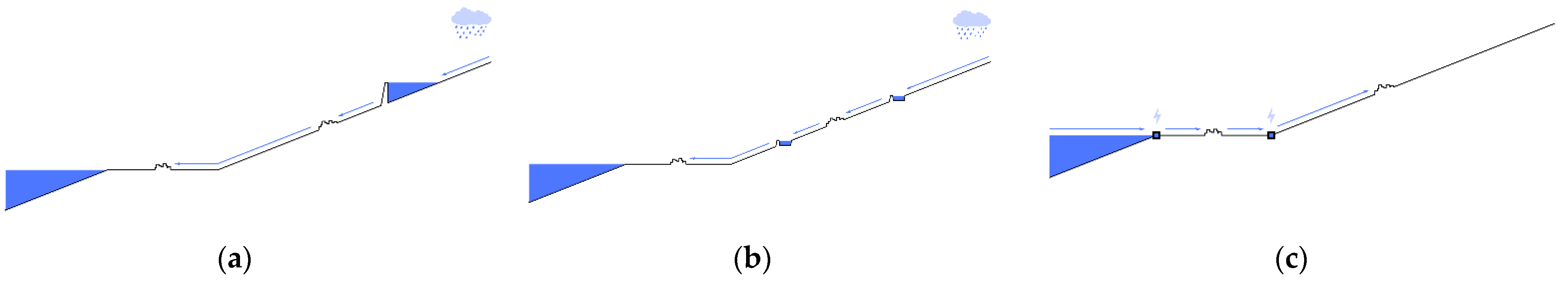
In the 1st solution, a dam is suggested to be built along the Nedontas river (
Figure 6a). An appropriate position for a dam has been chosen, such that the catchment area is adequate to meet the water needs, and such that the ground is of low permeability [
97]. The water is stored for up to a few years and then is transported via pipelines through a gravity-operated system (
Figure 7a).
In the 2nd solution, water ponds are suggested to be built at convenient locations above the settlements, so that water is captured at appropriate positions from local streams (
Figure 6b). It is then considered to be transported via pipelines to a number of water ponds, where it can be stored for up to a few months until its use (
Figure 7b). This system can be also gravity-operated.
In the 3rd solution, the option of seawater desalination was studied, where the desalinated process is implemented via reverse osmosis in several coastal desalination plants (
Figure 6c). Afterwards, it is considered to be pumped uphill to the settlements (
Figure 7c), where it can be stored for up to a few hours before its consumption.
Although all three solutions were technically feasible, they had different cash flow values. This means that in order to properly compare the cost of the solutions, a different approach is required, and a full analysis is needed to be conducted on the cost of water assuming a variable IR.
5.3. Estimating the Cost
To calculate the overall cost of water, we examined the cost of every solution individually. In the first solution with the dam, we identified three individual components:
- 8.
Dam construction [
98,
99], (lifespan 50 years)
- 9.
Pipe network construction (lifespan 50 years).
- 10.
For the cost of construction, we examined recent similar dam projects in terms of height and width, and we reached the number of 14,000,000 €. For the pipe-network, we calculated the cost to be 300 €/km for a 42 km pipeline. Finally, the total annual maintenance cost is 0.2% of the construction cost. The duration of the construction was assumed to be four years.
In the second solution with the water ponds, we identified two cost items:
- 11.
Ponds construction [
101] (lifespan 50 years).
- 12.
Pipe network construction (lifespan 50 years).
The pond construction cost was determined by using empirical equations that considered the size of the ponds. For the seven ponds, the total cost was estimated at around 2,000,000 €. The pipeline infrastructure cost was calculated to be 6,400,000 €. The duration of construction was assumed to be two years.
In the 3rd solution, we identified six cost items:
- 13.
Desalination plant construction and equipment [
102] (lifespan 25 years)
- 14.
Desalination plant maintenance [
103]
- 15.
Pipe network (lifespan 50 years)
- 16.
Pumping equipment (lifespan 25 years)
- 17.
Electricity for desalination [
104,
105] (electricity cost: 0.15 €/kwh)
- 18.
Electricity for pumping (electricity cost: 0.15 €/kwh)
Overall capital equipment (desalination plants and pumps) was 9.9 mil € (to be paid twice over 50 years), the pipe network 2,800,000 €, and operational annual costs 1,300,000 of which 1,000,000 corresponded just for the electricity. The duration of construction was assumed to be one year.
A general observation is that the operational costs of the desalination solution are immense, even if those are calculated with the assumption of very low energy prices. The cost of the pipe-network infrastructure in the dam exceeds the cost of the dam itself due to the distance covered; a vital observation regarding the importance of using local sources of water when possible. Finally, the cost of the pond construction was, surprisingly, quite small. In this case, even though there are diseconomies of scale (seven small ponds are more expensive than a large one), water ponds by nature are not mechanically complex and do not intercept the flow of the river to demand special attention from a structural and ecological point of view. They are, therefore, less expensive.
Subsequently, should the IR change significantly, the overall cost will change. Due to the fact that we treat water infrastructure costs and revenues as a cashflow timeseries (instead of a single value independent of time), the cost of water depends not on the average IR but rather on the behavior of the IR over time, as identified from the analysis of the synthetic timeseries. Over time, the unit cost of water will certainly change, and this shall be considered in the decision-making process.
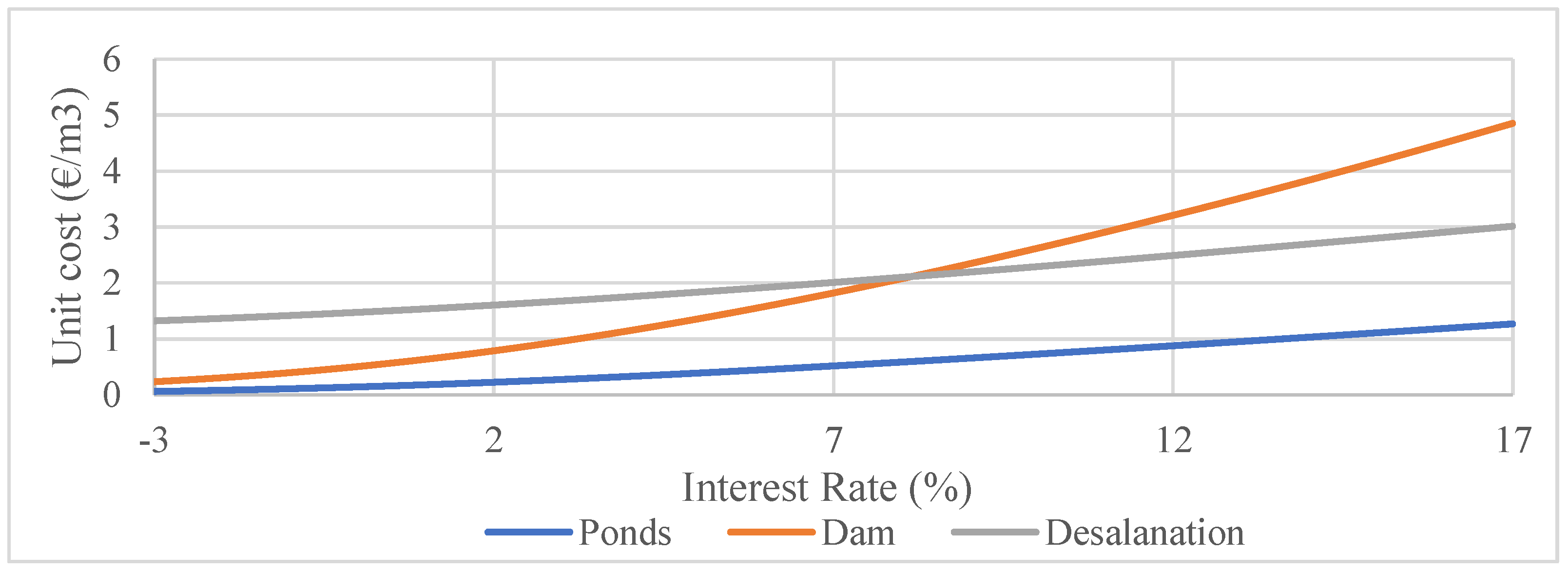
At first, we estimate the unit cost assuming a fixed IR between −3(%) to 17(%) [
106] (
Figure 8). It should be noted that a discount rate of 7% is the mid-range discount rate suggested for government projects [
107]. The unit cost is calculated by using fixed IR to calculate the present value of all revenues, which is then equated with the present value of all revenues.
From the above, we see that the construction of ponds, in all cases, is the least expensive option. Interestingly, we observe that for an IR above 8.4%, desalination becomes cheaper than the solution with the dam. This can be attributed to the fact that the dam requires most of its expense upfront, while the desalination process requires exceptionally high operational costs (mostly electricity costs). Therefore, should any infrastructure proposal tolerate the high cost of capital, the solutions to be examined may be different than what conventional wisdom suggests.
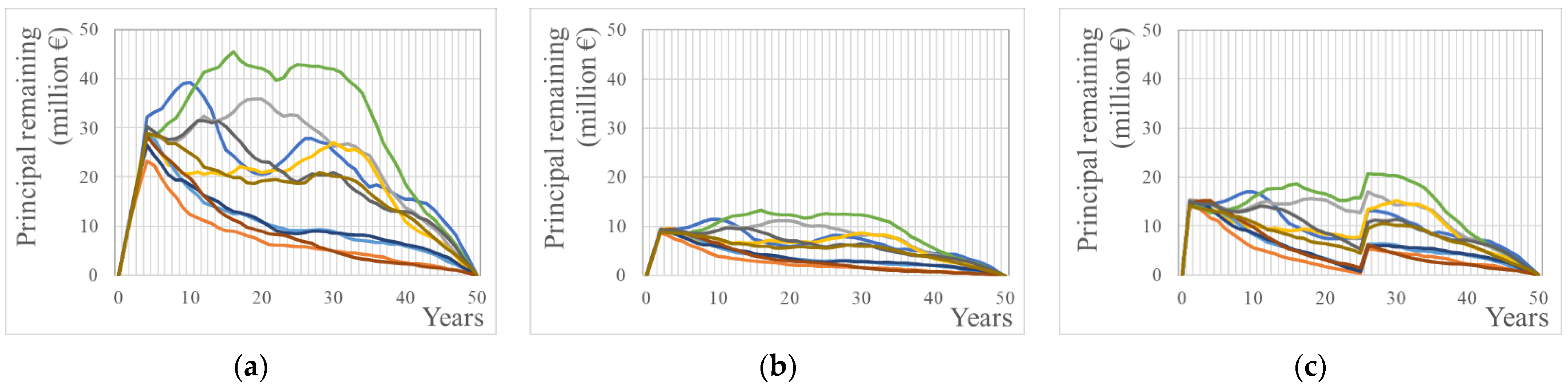
We then used the synthetic IR of Greece, and we simulated the three different solutions shown in
Figure 9, which depicts the emptying of the bathtub in
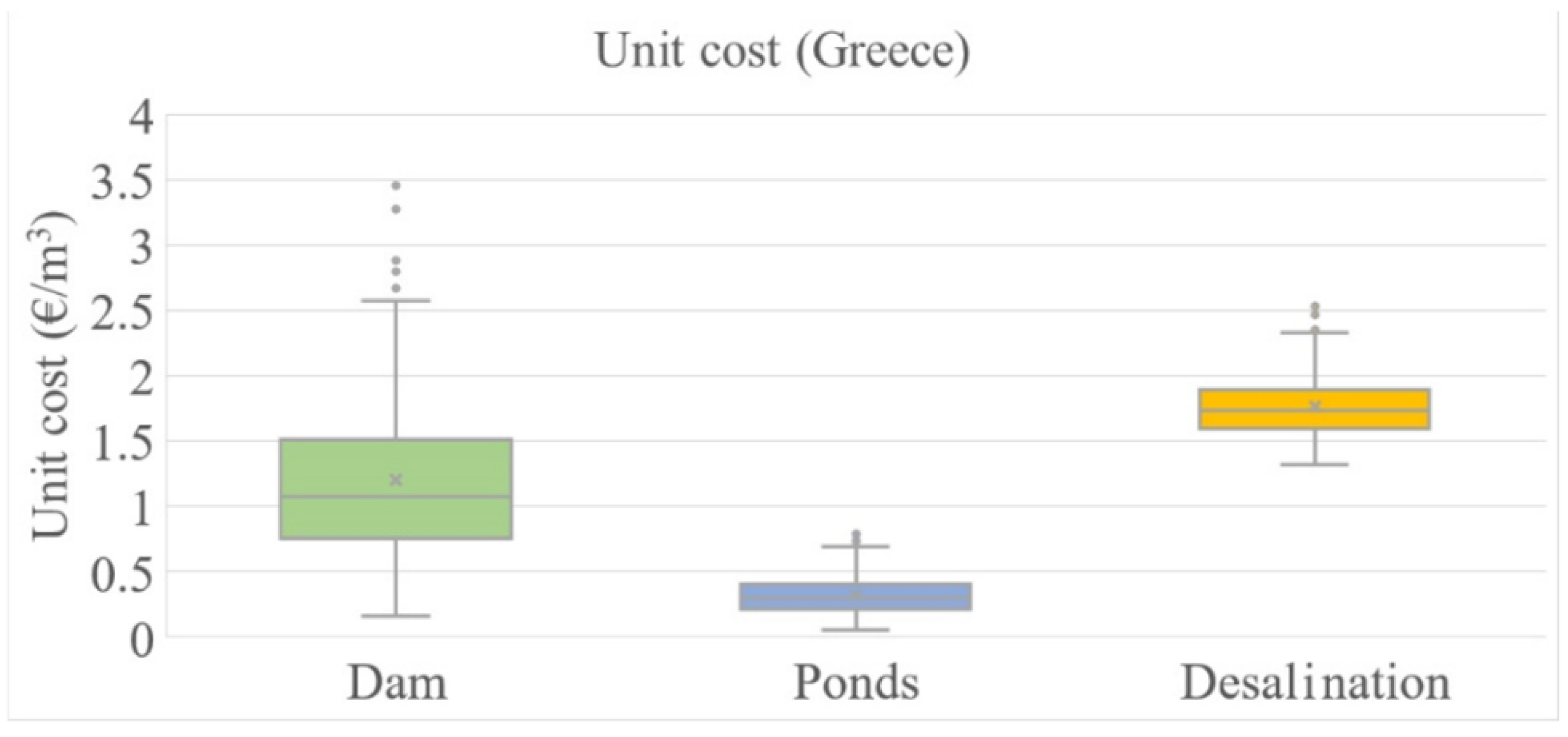
Figure 2. This was achieved with the following process: for each of the 200 synthetic timeseries we calculate the present value of all expenses, and we equate them to the present value of all revenues. Since every timeseries is unique, every present value is expected to be different (i.e., each unique timeseries produces a unique unit cost). The results and the associated distribution are depicted in
Figure 10.
We note that the second solution remains clearly the optimal one, as the unit cost, which is dependent on the cost of money, is clearly lower than the other two solutions, and with much smaller uncertainty. We should point out that the first solution presents the largest variance of outcomes. This can be attributed to the economic nature of each solution related to capital intensity. The high requirement of capital will expose the solution to the variance of the IR.
Figure 9.
Representative results of the stochastic simulation depicting principal remaining payments for different timeseries of the solution with the (a) dam, (b) ponds, and (c) desalination.
Figure 9.
Representative results of the stochastic simulation depicting principal remaining payments for different timeseries of the solution with the (a) dam, (b) ponds, and (c) desalination.
Figure 10.
Description of risk. Stochastic estimation of unit cost of each solution for Greece.
Figure 10.
Description of risk. Stochastic estimation of unit cost of each solution for Greece.
At this point, it should be obvious that by simulating each solution using synthetic IRs, we can extract useful observations regarding the economic nature of each solution, which may not have been obvious if we used the conventional method of a fixed IR.
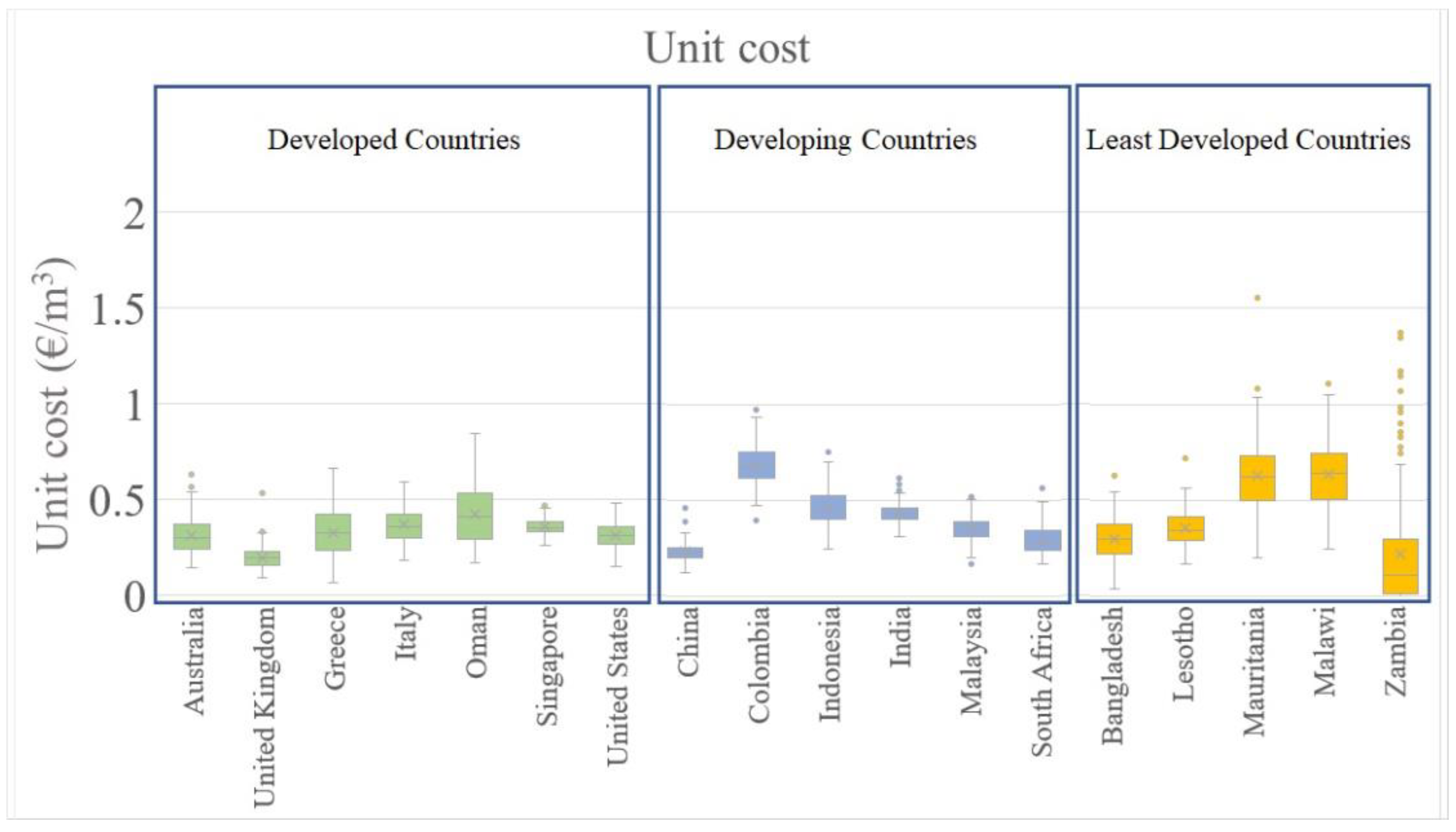
6. Global Evaluation of the Optimum Solution
Previous analysis examined the unit cost by using observed IR data from Greece. In this section, we will examine the unit cost of the preferred solution (ponds) in other countries, which have various levels of economic development. To do so, we used the historical real IR data from each of the selected countries to produce synthetic timeseries that we can then use to estimate the cost of the unit of the optimum solution.
There is no standard methodology to determine whether a country is developed, developing, or undeveloped; however, this characterization can be comparative. We choose to create the following criteria to determine the level of development in an individual country:
We choose the above criteria based on the belief that those compile many hidden nuances as opposed to the use of a single criterium such as GDP per capita. The development stage depends on various factors such as technical advancements, economic diversification, reliance on exports and imports, education, etc.
As we can see in
Figure 11, developed and developing countries do not produce substantially different results.
However, the least developed countries produce extremely unstable outcomes. This extreme volatility is caused by the volatility of the IR. Therefore, we can confirm that economic uncertainty can result in high-risk long-term investments in the least developed countries. This creates a «φαύλος κύκλος» (which is described also as a “catch-22”) situation in which long-term investments cannot be made due to the unstable economy, and by not conducting these investments, the economy remains undeveloped, and therefore, unstable with high variation of Irs.
7. Discussion
During this work, a geopolitical event took place; Russia’s ongoing special military operation in Ukraine (24 February 2022). The assumptions in our calculations considered a price of electricity at 0.15 €/kWh. This was already approximately three times higher than the decade average. However, the geopolitical unrest impacted fuel supplies and, subsequently, the price of electricity. We consider the price of electricity a new, extremely volatile variable, which can overturn previous conclusions. Thus, we recommend further research to be conducted with stochastic simulations taking into account the price of electricity as an additional stochastic variable. The current Markovian framework cannot host such large-scale changes in stochastic simulation, and a Hurst-Kolmogorov framework would be more appropriate to be implemented.
In a previous study [
89], we conducted a multi-criteria analysis in order to choose the optimal solution. However, the capital intensity was not considered. Though we quantified to a certain extent that factor in this paper in the form of the variability of the unit cost, we did not consider it at first. Rather, the first thought to select the least complicated local solution, was proven an unexpectedly neat choice.
In the introduction, we insinuated the importance of the water-energy-food Nexus. The place of water infrastructure is obviously very important in the Nexus. Of the three solutions, the option of desalination is the one with electricity requirements, which in turn increases the complexity of the Nexus. On the other hand, it just so happens that the solutions of the dam and the ponds will have an impact on food production, since surplus water could be directed to the water-starved agricultural production of the area. Ultimately, unless the Nexus is remarkably durable, we would recommend the dismissal of the solution of the desalination based on the dependency on electricity alone.
The scale of the three proposed solutions is very clear. The first solution (dam) is one of the largest scales since it involves a large infrastructure project requiring long-distance water transport and huge upfront costs. The second solution (ponds) is one of a medium scale in terms of the physical size of the infrastructure, but the smallest in terms of capital cost. The medium-sized footprint and small upfront costs make it a deceptively ‘light’ solution. The third solution (desalination) is the one of the smallest physical scales. The very limited land use requirements and the very small distance covered for every drop of water, make it extremely attractive in theory. Yet, its mechanical complexity and energy requirements make it unattractive in the end.
To further investigate the three above solutions, we examine the economics of their technical characteristics. The large-scale technical solution, which is the constructing of a dam, requires large amounts of capital that may introduce high uncertainty in the output results. Also, desalination requires electricity, which makes the solution expensive, and regarding the current sociopolitical situation, it can be concluded that this is not quite predictable in terms of the range of costs.
In addition, we observe that countries with different economic regimes produce multiple outcomes of the unit cost. We note that the least developed countries produce an expensive and wide range of outcomes. It is obvious that researchers should use data from their own countries, but in an increasingly interconnected world, the study of other neighboring or otherwise similar developmental countries, may give an additional useful point of view to decision-makers.
This research is significantly limited, as it did not conduct calculations using historical IR before 1945. Therefore, it is restricted to the post World War II (WWII) and before the current severe conflict in terms of its conclusions.
Given the extraordinary recent geopolitical events [
9] and their macroeconomic effects, in particular the abrupt rise of Irs in 2022 [
110] as well as inflation rates [
111], it is obvious that the recent 70-year trend of generally low and stable IR, which could be considered as a second “Bell Epoch”, is over. As a matter of fact, it seems that financial institutions have learned to operate in a stable financial environment, which in turn has made marginal large-scale projects viable.
To demonstrate this, we produced synthetic timeseries of the principal remaining for the United Kingdom (UK) using two datasets. The first uses data from the period 1907–1956, and the second from the period of 1961–2014 [
112,
113]. The first period includes two world wars (and the inter war period), which hit the UK particularly hard since it was a major belligerent and the most prominent imperial superpower at the time. We used those timeseries to simulate a theoretical capital-intensive construction in the UK (similar to the dam solution in our case study). The principal remaining for those two simulations are depicted in
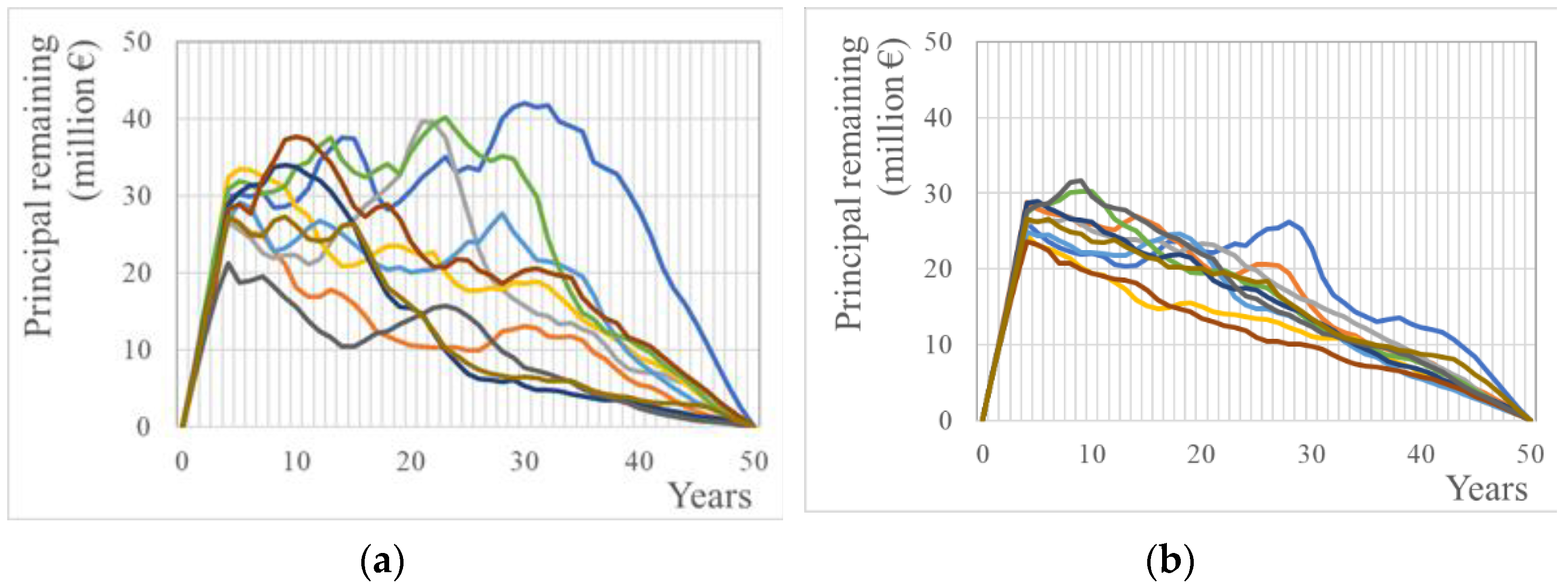
Figure 12. The results reveal the pattern of potential outcomes and those showing that higher and more unstable IR make public infrastructure projects very risky to finance in the economic conditions during a period of unrest. In particular, the standard deviation of the unit costs, for the simulation with data from the period of 1907–1956 is 0.347 compared to 0.212 when using data from 1961–2014. When it comes to water infrastructures, in particular, the failure to successfully fund them, could put the water-energy-food nexus in jeopardy.
Note that, when comparing the curves in
Figure 12a (data used from the UK 1907–1956) with
Figure 9a (data used from Greece 1961–2014), a similar spread is revealed (which means similar risk), since the political situation (and economic conditions) in Greece remained unstable in this period. This instability is also depicted in
Figure 11.
Figure 12.
Stochastic estimation of principal remaining for the construction of a dam using synthetic timeseries created (a) by data from 1907—1956 for the UK, and (b) by data from 1961–2014 for the UK.
Figure 12.
Stochastic estimation of principal remaining for the construction of a dam using synthetic timeseries created (a) by data from 1907—1956 for the UK, and (b) by data from 1961–2014 for the UK.
8. Conclusions
The main outcome of this work is the highlighting of the importance of the upfront cost (capital). Large capital requirements increase the cost of technical solutions and, importantly, exposure to the interest rate (IR) volatility. By default, the latter can be regarded as a macroeconomic vulnerability.
When making assumptions regarding a fixed IR, we suggest performing a sensitivity analysis with a range of values, at the very least. Different solutions may become viable at larger or smaller IRs.
Operational costs seem to have a large impact on infrastructure projects. The nature of operational costs is to distribute the overall cost over time to make a proposal attractive in specific cases.
Factors that can cause a lack of economic development can make a country’s investment opportunities challenging. The variability of outcomes is astonishing in countries that are on the list of the ‘least developed’ ones. To conclude, a country’s monetary stability is vital in order to make reasonably safe long-term investments.
In conclusion, the water-energy-food nexus should be considered as the real wealth (i.e., the foundations of society and not money itself). Moreover, the financial system should be organized so as to support the creation of economies of scale, since large-scale infrastructures may minimize the costs of the units that are the basis for social prosperity.
A period of military conflicts can result in extraordinarily high and variable IRs, which means a high risk of the finance of large-scale infrastructures. This instability hinders the construction of large-scale civil infrastructure which is vital for the prosperity of the society.
Author Contributions
Conceptualization, D.M., G.-F.S., T.I., P.D., N.M. and D.K. methodology, D.M., G.-F.S., T.I., P.D., N.M. and D.K. validation, D.M., G.-F.S., T.I., P.D., N.M. and D.K. formal analysis, D.M., G.-F.S., T.I., P.D., N.M. and D.K. investigation, D.M., G.-F.S., T.I., P.D., A.S., K.M., M.N., I.T.M., N.M. and D.K. data curation, D.M. writing—original draft preparation, D.M., G.-F.S., T.I. and P.D. writing—review and editing, T.I., P.D, N.M. and D.K., visualization, D.M., I.T.M. and G.-F.S., supervision D.K., project administration, G.-F.S. All authors have read and agreed to the published version of the manuscript.
Funding
The students involved in this research, namely D.M., A.S., K.M. and M.N. were funded by the Municipality of West Mani.
Institutional Review Board Statement
Not applicable.
Informed Consent Statement
Not applicable.
Data Availability Statement
The databases that have been used are referred to in detail in the citation given in the text and are publicly available.
Acknowledgments
We are grateful to the eponymous reviewers for their thoughtful and constructive comments that improved the manuscript. We thank the Municipality of West Mani for providing financial support to the students involved in this research.
Conflicts of Interest
The authors declare no conflict of interest.
References
- Gulati, M.; Jacobs, I.; Jooste, A.; Naidoo, D.; Fakir, S. The Water–energy–food Security Nexus: Challenges and Opportunities for Food Security in South Africa. Aquat. Procedia 2013, 1, 150–164. [Google Scholar] [CrossRef]
- Simpson, G.B.; Badenhorst, J.; Jewitt, G.; Berchner, M.; Davies, E. Competition for Land: The Water-Energy-Food Nexus and Coal Mining in Mpumalanga Province, South Africa. Front. Environ. Sci. 2019, 7, 86. [Google Scholar] [CrossRef]
- Yu, L.; Xiao, Y.; Zeng, X.; Li, Y.; Fan, Y. Planning water-energy-food nexus system management under multi-level and uncertainty. J. Clean. Prod. 2020, 251, 1343–1353. [Google Scholar] [CrossRef]
- Food and Agriculture Organization of United Nations. The Water-Energy-Food Nexus A New Approach in Support of Food Security and Sustainable Agriculture, Rome. 2014. Available online: http://www.fao.org/3/bl496e/bl496e.pdf (accessed on 28 June 2021).
- Sahlins, M. Stone Age Economics; Routledge: London, UK, 2013. [Google Scholar]
- Sargentis, G.-F.; Iliopoulou, T.; Sigourou, S.; Dimitriadis, P.; Koutsoyiannis, D. Evolution of Clustering Quantified by a Stochastic Method—Case Studies on Natural and Human Social Structures. Sustainability 2020, 12, 7972. [Google Scholar] [CrossRef]
- Sargentis, G.-F.; Iliopoulou, T.; Dimitriadis, P.; Mamassis, N.; Koutsoyiannis, D. Stratification: An Entropic View of Society’s Structure. World 2021, 2, 153–174. [Google Scholar] [CrossRef]
- Sargentis, G.-F.; Siamparina, P.; Sakki, G.-K.; Efstratiadis, A.; Chiotinis, M.; Koutsoyiannis, D. Agricultural Land or Photovoltaic Parks? The Water–Energy–Food Nexus and Land Development Perspectives in the Thessaly Plain, Greece. Sustainability 2021, 13, 8935. [Google Scholar] [CrossRef]
- Sargentis, G.F.; Lagaros, N.D.; Cascella, G.L.; Koutsoyiannis, D. Threats in Water–Energy–Food–Land Nexus by the 2022 Military and Economic Conflict. Land 2022, 11, 1569. [Google Scholar] [CrossRef]
- Smith, A. The Wealth of Nations; W. Strahan and T. Cadell: London, UK, 1776. [Google Scholar]
- O’Sullivan, A.; Sheffrin, S.M. Economics: Principles in Action; Pearson Prentice Hall: Upper Saddle River, NJ, USA, 2013; p. 157. ISBN 978-0-13-063085-8. [Google Scholar]
- Hanson, J.W.; Ortman, S.G.; Lobo, J. Urbanism and the division of labour in the Roman Empire. J. R. Soc. Interface 2017, 14, 20170367. [Google Scholar] [CrossRef]
- Buchan, J.M. The Division of Labor in the Economy, The Return to Increasing Returns; Buchanan, J.M., Yoon, Y.J., Eds.; The University of Michigan Press: Ann Arbor, MI, USA, 1994; Available online: https://books.google.gr/books?hl=en&lr=&id=d4yFu-yVn1AC&oi=fnd&pg=PA3&ots=z46SXomMXl&sig#v=onepage&q&f=false (accessed on 2 December 2022).
- Koutsoyiannis, D. Scale of water resources development and sustainability: Small is beautiful, large is great. Hydrol. Sci. J. 2011, 56, 553–575. [Google Scholar] [CrossRef]
- Koutsoyiannis, A. Modern Microeconomics, 2nd ed.; Springer: London, UK, 1979. [Google Scholar]
- Xanthopoulos, T. Requiem with Crescendo? Homo Sapiens the Ultimate Genus of Human, Volume A; National Technical University of Athens: Athens, Greece, 2017. (In Greek) [Google Scholar]
- Koutsoyiannis, D.; Sargentis, G.-F. Entropy and Wealth. Entropy 2021, 23, 1356. [Google Scholar] [CrossRef]
- Angelakis, A.N.; Kavoulaki, E.; Dialynas, M.G. Sanitation and Stormwater and Wastewater Technologies in Minoan Era. In Evolution of Sanitation and Wastewater Management through the Centuries; Angelakis, A., Rose, J., Eds.; IWA Publishing: London, UK, 2014; Chapter 1; pp. 1–24. [Google Scholar]
- Sargentis, G.-F.; Koutsoyiannis, D.; Angelakis, A.; Christy, J.; Tsonis, A.A. Environmental Determinism vs. Social Dynamics: Prehistorical and Historical Examples. World 2022, 3, 357–388. [Google Scholar] [CrossRef]
- Baillie, R.T. Long memory processes and fractional integration in econometrics. J. Econ. 1996, 73, 5–59. [Google Scholar] [CrossRef]
- Peng, C.-K.; Buldyrev, S.V.; Goldberger, A.L.; Havlin, S.; Sciortino, F.; Simons, M.; Stanley, H.E. Long-range correlations in nucleotide sequences. Nature 1992, 356, 168–170. [Google Scholar] [CrossRef] [PubMed]
- Voss, R.F.; Clarke, J. ‘1/fnoise’ in music and speech. Nature 1975, 258, 317–318. [Google Scholar] [CrossRef]
- Ellaway, P. Cumulative sum technique and its application to the analysis of peristimulus time histograms. Electroencephalogr. Clin. Neurophysiol. 1978, 45, 302–304. [Google Scholar] [CrossRef]
- Kolmogorov, A.N. A refinement of previous hypotheses concerning the local structure of turbulence in a viscous incompressible fluid at high Reynolds number. J. Fluid Mech. 1962, 13, 82–85. [Google Scholar] [CrossRef] [Green Version]
- Sargentis, G.-F.; Dimitriadis, P.; Koutsoyiannis, D. Aesthetical Issues of Leonardo Da Vinci’s and Pablo Picasso’s Paintings with Stochastic Evaluation. Heritage 2020, 3, 283–305. [Google Scholar] [CrossRef]
- Sargentis, G.-F.; Dimitriadis, P.; Iliopoulou, T.; Koutsoyiannis, D. A Stochastic View of Varying Styles in Art Paintings. Heritage 2021, 4, 333–348. [Google Scholar] [CrossRef]
- Butcher, K.; Ponting, M. The Beginning of the End? The Denarius in the Second Century. Numis. Chron. 2012, 172, 63–83. Available online: http://www.jstor.org/stable/42678930 (accessed on 2 December 2022).
- Sargentis, G.-F.; Defteraios, P.; Lagaros, N.D.; Mamassis, N. Values and Costs in History: A Case Study on Estimating the Cost of Hadrianic Aqueduct’s Construction. World 2022, 3, 260–286. [Google Scholar] [CrossRef]
- Norges Bank. The Role of the Interest Rate in the Economy. 19 October 2003. Available online: https://www.norges-bank.no/en/news-events/news-publications/Speeches/2003/2003-10-19/#:~:text=Interest%20is%20therefore%20also%20the,responsibility%20of%20the%20central%20bank (accessed on 2 December 2022).
- Banton, C. Interest Rate, Investopedia. 6 July 2022. Available online: https://www.investopedia.com/terms/i/interestrate.asp (accessed on 2 December 2022).
- European Central Bank. Benefits of Price Stability. Available online: https://www.ecb.europa.eu/mopo/intro/benefits/html/index.en.html (accessed on 2 December 2022).
- Adam, K.; Junyi, Z. Price Level Changes and the Redistribution of Nominal Wealth Across the Euro Area. J. Eur. Econ. Assoc. 2014, 14, 871–906. [Google Scholar] [CrossRef]
- LePan, N. The History of Interest Rates Over 670 Years. Visual Capitalist. 15 November 2019. Available online: https://www.visualcapitalist.com/the-history-of-interest-rates-over-670-years/ (accessed on 28 October 2022).
- Cox, J.C.; Ingersoll, J.E.; Ross, S.A. A Theory of the Term Structure of Interest Rates. Econometrica 1985, 53, 385. [Google Scholar] [CrossRef]
- Ingersoll, J.E., Jr.; Ross, S.A. Waiting to Invest: Investment and Uncertainty. J. Bus. 1992, 65, 1–29. [Google Scholar] [CrossRef]
- Zenios, S. A model for portfolio management with mortgage-backed securities. Ann. Oper. Res. 1993, 43, 337–356. [Google Scholar] [CrossRef]
- Munk, C.; Rubtsov, A. Portfolio management with stochastic interest rates and inflation ambiguity. Ann. Finance 2013, 10, 419–455. [Google Scholar] [CrossRef] [Green Version]
- Pearl, R.L.; Hopkins, C.H.; Berkowitz, R.I.; Wadden, T.A. Group cognitive-behavioral treatment for internalized weight stigma: A pilot study. Eat Weight Disord. 2018, 23, 357–362. [Google Scholar] [CrossRef]
- Deelstra, G.; Delbaen, F. Long-term returns in stochastic interest rate models. Insur. Math. Econ. 1995, 17, 163–169. [Google Scholar] [CrossRef] [Green Version]
- Eisenberg, J. Optimal dividends under a stochastic interest rate. Insur. Math. Econ. 2015, 65, 259–266. [Google Scholar] [CrossRef]
- Zaglauer, K.; Bauer, D. Risk-neutral valuation of participating life insurance contracts in a stochastic interest rate environment. Insur. Math. Econ. 2008, 43, 29–40. [Google Scholar] [CrossRef] [Green Version]
- Yao, H.; Li, Z.; Li, D. Multi-period mean-variance portfolio selection with stochastic interest rate and uncontrollable liability. Eur. J. Oper. Res. 2016, 252, 837–851. [Google Scholar] [CrossRef]
- Shevchenko, P.V.; Luo, X. Valuation of variable annuities with Guaranteed Minimum Withdrawal Benefit under stochastic interest rate. Insur. Math. Econ. 2017, 76, 104–117. [Google Scholar] [CrossRef]
- Tolis, A.; Doukelis, A.; Tatsiopoulos, I. Stochastic interest rates in the analysis of energy investments: Implications on economic performance and sustainability. Appl. Energy 2009, 87, 2479–2490. [Google Scholar] [CrossRef]
- Park, C.; Park, P.-K.; Mane, P.P.; Hyung, H.; Gandhi, V.; Kim, S.-H.; Kim, J.-H. Stochastic cost estimation approach for full-scale reverse osmosis desalination plants. J. Membr. Sci. 2010, 364, 52–64. [Google Scholar] [CrossRef]
- Guerrini, A.; Romano, G.; Leardini, C. Economies of scale and density in the Italian water industry: A stochastic frontier approach. Util. Policy 2018, 52, 103–111. [Google Scholar] [CrossRef]
- Khaligh, V.; Anvari-Moghaddam, A. Stochastic expansion planning of gas and electricity networks: A decentralized-based approach. Energy 2019, 186, 1–11. [Google Scholar] [CrossRef]
- Zhang, Q.; Guo, X.; Li, H. The Impact of Financial Risks on Financial Investment in Infrastructure: Based on a Two-Factor Stochastic Differential Equation. Discret. Dyn. Nat. Soc. 2021, 2021, 1–14. [Google Scholar] [CrossRef]
- Katz, Y.A. Value of the distant future: Model-independent results. Phys. A Stat. Mech. its Appl. 2017, 466, 269–276. [Google Scholar] [CrossRef]
- Dacuycuy, L.; Sauler, M.M.; Lim, D. On Implementation Delays, Marginal Costs and Price Dynamics: A Theoretical Note with Implications for the Philippines1. DLSU Bus. Econ. Rev. 2019, 28, 87–103. [Google Scholar]
- Michel, J.-B.; Shen, Y.K.; Aiden, A.P.; Veres, A.; Gray, M.K.; Pickett, J.P.; Hoiberg, D.; Clancy, D.; Norvig, P.; Orwant, J.; et al. Quantitative Analysis of Culture Using Millions of Digitized Books. Science 2011, 331, 176–182. [Google Scholar] [CrossRef] [Green Version]
- Scopus. Scopus Database. Available online: https://www.scopus.com/ (accessed on 1 December 2021).
- Hemming, G. Interest Rate Definition in Economics: From Real to Nominal IR. ABC Finance Limited. Available online: https://abcfinance.co.uk/loan/interest/rate/ (accessed on 25 July 2022).
- Definition of Cost of Money, Merriam-Webster Dictionary. Available online: https://www.merriam-webster.com/dictionary/cost%20of%20money (accessed on 22 September 2022).
- Blank, L.T.; Tarquin, A.J. Engineering Economy; McGraw-Hill: New York, NY, USA, 2012; Available online: https://www.hzu.edu.in/engineering/engineering%20economy.pdf (accessed on 25 July 2022).
- Fisher Equation, Corporate Finance Institute. Available online: https://corporatefinanceinstitute.com/resources/knowledge/economics/fisher-equation/ (accessed on 22 September 2022).
- Principles of Managerial Finance, 10th ed.; Lawrence J. Gitman: Boston, MA, USA, 2010.
- Office of Management and Budget Circular A-94: Guidelines and Discount Rates for Benefit-Cost Analysis of Federal Program. 29 October 1992. Available online: https://obamawhitehouse.archives.gov/sites/default/files/omb/assets/a94/a094.pdf (accessed on 20 September 2022).
- Jawad, D.; Ozbay, K. The Discount Rate in Life Cycle Cost Analysis of Transportation Projects; National Academy of Science: Washington, DC, USA, 2005. [Google Scholar]
- Walter, I. (Ed.) 7. Infrastructure Finance. In The Infrastructure Finance Challenge: A Report by the Working Group on Infrastructure Finance Stern School of Business; Walter, I. (Ed.) New York University; Open Book Publishers: New York, NY, USA, 1991; Available online: http://books.openedition.org/obp/3366 (accessed on 2 December 2022).
- Committee for a Responsible Federal Budget ‘How Would Higher Interest Rates Affect Interest Payments? Available online: https://www.crfb.org/blogs/how-would-higher-interest-rates-affect-interest-payments (accessed on 20 September 2022).
- Buchanan, J.M. Opportunity Cost. 1991, pp. 520–525. Available online: https://link.springer.com/chapter/10.1007/978-1-349-21315-3_69 (accessed on 20 September 2022).
- Hawkins, J. Economic forecasting: History and procedures. Econ. Round-Up J. Dep. Treasury. 2005, 1–10. Available online: https://researchprofiles.canberra.edu.au/en/publications/economic-forecasting-history-and-procedures (accessed on 20 September 2022).
- Bratt, E.C.; Cox, G.V. An Appraisal of American Business Forecasts. J. Am. Stat. Assoc. 1930, 25, 383. [Google Scholar] [CrossRef]
- Tornado Forecasters Are Closing in on the Theoretical Limit of Prediction-Accuracy’, The Atlantic. Available online: https://www.theatlantic.com/national/archive/2014/04/tornado-forecasters-are-closing-in-on-the-theoretical-limit-of-prediction-accuracy/361314/ (accessed on 20 September 2022).
- Armstrong, J.S. Standards and Practices for Forecasting. 2001, pp. 679–732. Available online: https://link.springer.com/chapter/10.1007/978-0-306-47630-3_31 (accessed on 20 September 2022).
- Winston, W.L. Operations Research, Applications and Algorithms, 3rd ed.; Duxbury Publisher: London, UK, 1994. [Google Scholar]
- Armstrong, J.S. Long-Range Forecasting from Crystal Ball to Computer, 2nd ed.; John Wiley & Sons: Hoboken, NJ, USA, 1985; pp. 408–409. [Google Scholar]
- Fildes, R. A Quantitative forecasting—The state of the art: Econometric models. J. Opera-Tional Res. Soc. 1985, 36, 572–574. [Google Scholar]
- Bailey, A.L. A Summary of Advanced Statistical Methods; United Fruit Company: Boston, MA, USA, 1929; Available online: https://babel.hathitrust.org/cgi/pt?id=mdp.39015067991326&view=1up&seq=7 (accessed on 27 October 2022).
- World Bank, Real Interest Rates (%), 1960–2021. Available online: https://api.worldbank.org/v2/en/indicator/FR.INR.RINR?downloadformat=excel (accessed on 21 October 2022).
- Ksendal, B.K. Stochastic Differential Equations: An Introduction with Applications; Springer: Berlin/Heidelberg, Germany; New York, NY, USA, 2003. [Google Scholar]
- Koutsoyiannis, D. Univariate Stationary Stochastic Models; Lecture Notes on Stochastic Methods; School of Civil Engineering National Technical University of Athens: Athens, Greece, 2017; Available online: https://www.itia.ntua.gr/en/docinfo/1742/ (accessed on 2 December 2022).
- Box, G.; Jenkins, J.; Reinsel, G. Time Series Analysis: Forecasting and Control, 3rd ed.; Prentice Hall: Upper Sad-dle River, NJ, USA, 1994. [Google Scholar]
- Damodaran, A. Macroeconomic Data. Available online: https://pages.stern.nyu.edu/~adamodar/New_Home_Page/ (accessed on 22 February 2022).
- Sargentis, G.-F.; Ioannidis, R.; Karakatsanis, G.; Koutsoyiannis, D. The Scale of Infrastructures as a Social Decision. Case Study: Dams in Greece; European Geosciences Union General Assembly: Vienna, Austria, 2018; Available online: https://www.itia.ntua.gr/en/docinfo/1812/ (accessed on 2 December 2022).
- Markantonis, D.; Moraiti, K.; Nikolinakou, M.; Siganou, A. Water Supply for the Municipality of Western Mani; Department of Water Resources and Environmental Engineering—National Technical University of Athens: Athens, Greece, 2022; Available online: https://www.itia.ntua.gr/en/docinfo/2244/ (accessed on 24 February 2022).
- Iliopoulou, T.; Dimitriadis, P.; Siganou, A.; Markantonis, D.; Moraiti, K.; Nikolinakou, M.; Meletopoulos, I.T.; Mamassis, N.; Koutsoyiannis, D.; Sargentis, G.-F. Modern Use of Traditional Rainwater Harvesting Practices: An Assessment of Cisterns’ Water Supply Potential in West Mani, Greece. Heritage 2022, 5, 2944–2954. [Google Scholar] [CrossRef]
- Seifried, R.M.; Gardner, C.A.M. Maintaining Distinction: Local Identity in the Remote Mani Peninsula, Greece, in the Classical, Byzantine, and Ottoman Periods. In Proceedings of the Joint Annual Meeting of the Archaeological Institute of America and the Society for Classical Studies, New Orleans, LA, USA, 8–11 January 2015; Available online: https://www.academia.edu/10144387/Maintaining_Distinction_Local_Identity_in_the_Remote_Mani_Peninsula_Greece_in_the_Classical_Byzantine_and_Ottoman_Periods (accessed on 2 December 2022).
- Koutsoyiannis, D.; Angelakis, A.N. Agricultural Hydraulic Works in Ancient Greece, Encyclopedia of Water Science, 2nd ed.; Trimble, S.W., Ed.; CRC Press Taylor & Francis Group: London, UK; New York, NJ, USA, 2007; pp. 24–27. [Google Scholar]
- Angelakis, A.N.; Koutsoyiannis, D. Urban water engineering and management in ancient Greece. In Encyclopedia of Water Science; Stewart, B.A., Howell, T., Eds.; Dekker: New York, NY, USA, 2003; pp. 999–1007. [Google Scholar]
- Koutsoyiannis, D.; Angelakis, A.N. Hydrologic and hydraulic science and technology in ancient Greece. In Encyclopedia of Water Science; Stewart, B.A., Howell, T., Eds.; Dekker: New York, NY, USA, 2003; pp. 415–417. [Google Scholar]
- Angelakis, A.N.; Spyridakis, D.S. A brief history of water supply and wastewater management in ancient Greece. Water Supply 2010, 10, 618–628. [Google Scholar] [CrossRef]
- Stedman, N. Land use and settlement in post-Medieval Central Greece: An interim discussion. In The Archaeology of Medieval Greece; Lock, P., Sanders, G.D.R., Eds.; Oxbow: Oxford, UK, 1996; pp. 179–192. [Google Scholar]
- Angelakis, A.N.; Koutsoyiannis, D.; Tchobanoglous, G. Urban wastewater and stormwater technologies in ancient Greece. Water Res. 2005, 39, 210–220. [Google Scholar] [CrossRef]
- Sargentis, G.-F.; Dimitriadis, P.; Ioannidis, R.; Iliopoulou, T.; Frangedaki, E.; Koutsoyiannis, D. Optimal utilization of water resources for local communities in mainland Greece (case study of Karyes, Peloponnese). Procedia Manuf. 2020, 44, 253–260. [Google Scholar] [CrossRef]
- Mamassis, N.; Chrysoulaki, S.; Bendermacher-Geroussis, E.; Evangelou, T.; Koutis, P.; Peppas, G.; Defteraios, P.; Zarkadoulas, N.; Koutsoyiannis, D.; Griva, E. Representing the operation and evolution of ancient Piraeus’ water supply system. Water Hist. 2022, 14, 123–144. [Google Scholar] [CrossRef]
- Tsiouri, C. Hydraulic Investigation of the Adrian Aqueduct. Master’s Thesis, Department of Water Resources and Environment, Shool of Civil Engineering, National Technical University of Athens, Athens, Greece, October 2018. Available online: https://www.itia.ntua.gr/el/docinfo/1913/ (accessed on 25 January 2022).
- Moraiti, K.; Markantonis, D.; Nikolinakou, M.; Siganou, A.; Sargentis, G.-F.; Iliopoulou, T.; Dimitriadis, P.; Meletopoulos, I.T.; Mamassis, N.; Koutsoyiannis, D. Optimizing Water Infrastructure Solutions for Small-Scale Dis-Tributed Settlements—Case Study at the Municipality of Western Mani; European Geosciences Union General Assembly: Vienna, Austria, 2022. [Google Scholar] [CrossRef]
- Markantonis, D.; Siganou, A.; Moraiti, K.; Nikolinakou, M.; Sargentis, G.-F.; Iliopoulou, T.; Dimitriadis, P.; Meletopoulos, I.T.; Mamassis, N.; Koutsoyiannis, D. Determining Optimal Scale of Water Infrastructure Considering Economical Aspects with Stochastic Evaluation—Case Study; Western Mani. European Geo-sciences Union General Assembly: Vienna, Austria, 2022. [Google Scholar] [CrossRef]
- Meteo Precipitation Data. Available online: https://meteosearch.meteo.gr/ (accessed on 20 September 2022).
- Precipitation Data. Available online: https://climexp.knmi.nl/selectstation.cgi?id=someone%40somewhere&fbclid=IwAR3TPNvvXLa9EtWYs1ctfFZgqc3s0p7ezzbMoK7kX5lHDkkMImMibpX1qo0 (accessed on 20 September 2022).
- Dimitriadis, P.; Koutsoyiannis, D.; Tzouka, K. Predictability in dice motion: How does it differ from hydro-meteorological processes? Hydrol. Sci. J. 2016, 61, 1611–1622. [Google Scholar] [CrossRef] [Green Version]
- Koutsoyiannis, D. A random walk on water. Hydrol. Earth Syst. Sci. 2010, 14, 585–601. [Google Scholar] [CrossRef] [Green Version]
- Dimitriadis, P.; Koutsoyiannis, D.; Iliopoulou, T.; Papanicolaou, P. A Global-Scale Investigation of Stochastic Similarities in Marginal Distribution and Dependence Structure of Key Hydrological-Cycle Processes. Hydrology 2021, 8, 59. [Google Scholar] [CrossRef]
- Siganou, A.; Nikolinakou, M.; Markantonis, D.; Moraiti, K.; Sargentis, G.-F.; Iliopoulou, T.; Dimitriadis, P.; Cio-tinis, M.; Mamassis, N. Stochastic Simulation of Hydrological Timeseries for Data Scarce Regions—Case Study at the Municipality of Western Mani; European Geosciences Union General Assembly: Vienna, Austria, 2022. [Google Scholar] [CrossRef]
- Zogakis, C. Comparison of Event-Based and Continuous Simulation Models for the estimation of Flood Flows—Application to Nedontas River Basin. Master’s Thesis, Department of Water Resources and Environmental Engineerin, National Technical University of Athens, Athens, Greece, March 2013. Available online: https://www.itia.ntua.gr/en/docinfo/1327/ (accessed on 2 December 2022).
- Dams and Ponds of the Ministry of Agricultural Development and Food, Ministry of Agricultural Development and Food. 2006. Available online: https://www.ekke.gr/projects/estia/gr_pages/F_synerg/mikra%20fragmata_yp.georgias/mikra%20fragmata.pdf (accessed on 20 May 2022).
- Sako, Μ.; Tsoli, E.; Ioannidis, R.; Frangedaki, E.; Sargentis, G.-F.; Koutsoyiannis, D. Optimizing the Size of Hilarion Dam with Technical, Economical and Environmental Parameters; European Geosciences Union General Assembly: Vienna, Austria, 2019; Available online: https://www.itia.ntua.gr/en/docinfo/1947/ (accessed on 2 December 2022).
- Petheram, C.; McMahon, T. Dams, dam costs and damnable cost overruns. J. Hydrol. X 2019, 3, 100026. [Google Scholar] [CrossRef]
- Sargentis, G.-F.; Ioannidis, R.; Karakatsanis, G.; Sigourou, S.; Lagaros, N.D.; Koutsoyiannis, D. The Development of the Athens Water Supply System and Inferences for Optimizing the Scale of Water Infrastructures. Sustainability 2019, 11, 2657. [Google Scholar] [CrossRef] [Green Version]
- Zotalis, K.P. Energy and Economic Evaluation of Desalination Systems. Application in the Greek Area. Master’s Thesis, National Technical University of Athens, Athens, Greece, 2012. [Google Scholar] [CrossRef]
- Koykoytsakis, P.; Xatziargiriou, N. Impact of Desalination Loading to Island Energy System. Master’s Thesis, National Technical University of Athens, Athens, Greece, 2007. [Google Scholar]
- Zotalis, K.; Dialynas, E.G.; Mamassis, N.; Angelakis, A.N. Desalination Technologies: Hellenic Experience. Water 2014, 6, 1134–1150. [Google Scholar] [CrossRef] [Green Version]
- Tucker, D.; Marget, A.W.; Thompson, J.G. Appraisal of Economic Forecasts: Discussion. J. Am. Stat. Assoc. 1930, 25, 41. [Google Scholar] [CrossRef]
- Sensitivity Analysis, Investopedia. Available online: https://www.investopedia.com/terms/s/sensitivityanalysis.asp (accessed on 16 August 2022).
- Harrison, M. Valuing the Future: The Social Discount Rate in Costbenefit Analysis; Australian Government Productivity Commission: Canberra, Australia, 2010. Available online: https://www.pc.gov.au/research/supporting/cost-benefit-discount (accessed on 20 August 2022).
- World Bank Group. World Bank Country and Lending Groups; World Bank Group: Washington, DC, USA, 2018; Available online: https://datahelpdesk.worldbank.org/knowledgebase/articles/906519 (accessed on 4 July 2018).
- List of Least Developed Countries, United Nations. Available online: https://www.un.org/development/desa/dpad/least-developed-country-category/creation-of-the-ldc-category-and-timeline-of-changes-to-ldc-membership-and-criteria.html (accessed on 20 September 2022).
- Ross, J. Comparing the Speed of U.S. Interest Rate Hikes (1988–2022). 6 October 2022. Available online: https://www.visualcapitalist.com/comparing-the-speed-of-u-s-interest-rate-hikes/ (accessed on 30 October 2022).
- Consumer Prices, OECD—Updated: 6 September 2022. Available online: https://www.oecd.org/newsroom/consumer-prices-oecd-updated-6-september-2022.htm (accessed on 30 October 2022).
- St. Lois Federal Reserve. Consumer Price Inflation in the United Kingdom. Available online: https://fred.stlouisfed.org/series/CPIIUKA (accessed on 17 November 2022).
- St. Lois Federal Reserve. Consol (Long-Term Bond) Yields in the United Kingdom. Available online: https://fred.stlouisfed.org/series/LTCYUK (accessed on 17 November 2022).
| Disclaimer/Publisher’s Note: The statements, opinions and data contained in all publications are solely those of the individual author(s) and contributor(s) and not of MDPI and/or the editor(s). MDPI and/or the editor(s) disclaim responsibility for any injury to people or property resulting from any ideas, methods, instructions or products referred to in the content. |
© 2023 by the authors. Licensee MDPI, Basel, Switzerland. This article is an open access article distributed under the terms and conditions of the Creative Commons Attribution (CC BY) license (https://creativecommons.org/licenses/by/4.0/).


 ,
, 


