Development of a Speed Control Device for Fishing Vessels at Low Speeds and Simulation of the Control System

Abstract

Trawling is one of the most common fishing methods used by small vessels. This method requires the vessel to operate at a constant low speed because the depth of the trawl must be kept constant. In addition, the operation is often conducted by a small number of people, who must simultaneously maneuver the vessel and fish, making automation desirable. To develop this device, a mathematical model of the vessel was created based on data collected from actual operation of the vessel, and simulations were conducted to determine what type of control system would be suitable. As a result, it was possible to grasp effective control methods, effects of disturbances such as tides and waves, and how to deal with effective parts to improve response.

1. Introduction

1.1. Automatic Speed Control Systems

The aquaculture and fisheries sector is developing creative ways to meet the rapidly increasing human demand for nutrient-rich seafood by efficiently utilizing the planet’s vast water resources and aquatic biodiversity. This includes the progressive integration of information technology, data science, and artificial intelligence with fishing and aquaculture methods to enhance aquaculture production, sustainably develop natural fishery resources, and mechanize and automate related activities [1]. The various emerging technologies developed over the past decade include smart devices for collecting and sharing information over networks and emerging technologies such as the Internet of Things (IoT), often foreseen as the future solution for intelligent monitoring assemblies. Among others, automation is an important part of the new generation of information technology and represents the ultimate achievement in the development of marine surveillance programs [2,3]. In this paper, we focus on automated navigation in the current focus on maritime autonomous surface vessels (MASS) [4,5], which are not the large vessels that are commonly used, but rather on small vessels, such as in private fisheries, for the automated navigation of largehead hairtail fishing methods. In largehead hairtail fishing, fishing vessels need to be controlled at a constant low speed to maintain a constant net depth. To begin with, there are still few examples of automated navigation systems on small vessels in these fisheries studies. Indeed, to date, there have been studies that have investigated the optimization of energy efficiency and the control of autonomous vessels [6,7,8]. However, no research has been conducted specifically on small vessels that use automatic speed controllers and still require low speeds, such as trawl fishing vessels.

To develop an automatic speed controller, a ship model was created based on data collected from fishing vessel experiments, and simulations were conducted to determine what kind of control system would be suitable for the effects of tides and waves in actual sea conditions. Finally, we attempted to understand the optimal control method (proportional control, PI control, I-P control, and I-P + feedforward control), the effect on external disturbances, and effective areas for better response, to develop an automated trawl fishing method for the largehead hairtail fishery.

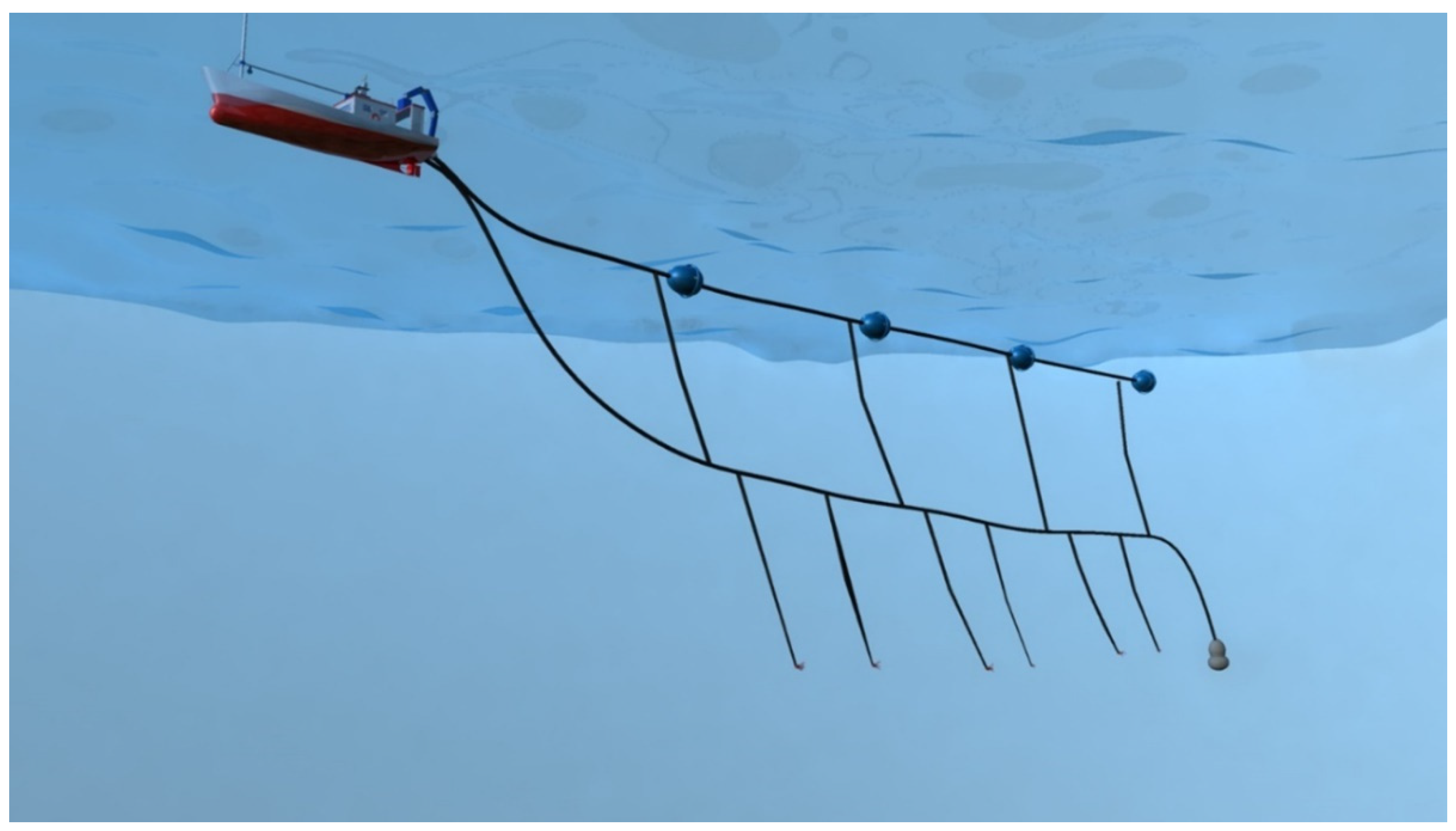
1.2. Trawl Fishing Methods

The extent to which bottom trawling impacts the marine environment continues to be debated [9,10,11]. Both the scale of trawling impacts and the ecological effects have been highlighted, suggesting that bottom trawlers cover an area equivalent to perhaps half of the world’s continental shelf each year [10]. A robust quantification of the distribution and intensity of bottom trawling provides a source of evidence to assess the pressure on seabed habitats, compare the impacts of different fisheries, characterize the fishery, and estimate the extent of unfished areas outside marine protected areas (MPAs) and fishing regulations [12,13,14,15,16,17]. An overview of the trawl fishery is shown in Figure 1. This paper focuses on improvements, especially in the technical aspects. In trawling, fish are detected by a fish finder and traps are lowered to the location of schools of fish. Lowering traps to the location of fish while maintaining a constant speed is conventionally performed manually and requires skill, especially in lowering traps at low speeds. This paper describes the automation of this process in order to reduce labor shortages in the fishing industry and improve fishing efficiency through technological improvements.

2. Objective

This experiment on the optimal speed control device for an automated trawl fishing method is named SLAFT (Shiraishi’s Low-speed Automation Fishing Experiments for Trawl). SLAFT emphasizes the importance of achieving a gradual speed at which fish can be secured. SLAFT aims to achieve the following items.

(1) To create a model of the fishing vessel (target of control) and investigate its validity.

(2) In the case of speed control, to examine effective control methods for the control target in response to input signals and external disturbances.

(3) After creating the model, the automatic control system should be confirmed by simulation. In this study, simulation experiments should be conducted using proportional control, PI control, I-P control, and I-P + feedforward control. In addition, various disturbances should be input to the control method that may be most suitable among these, and the effects of the disturbances should be observed.

3. Methods

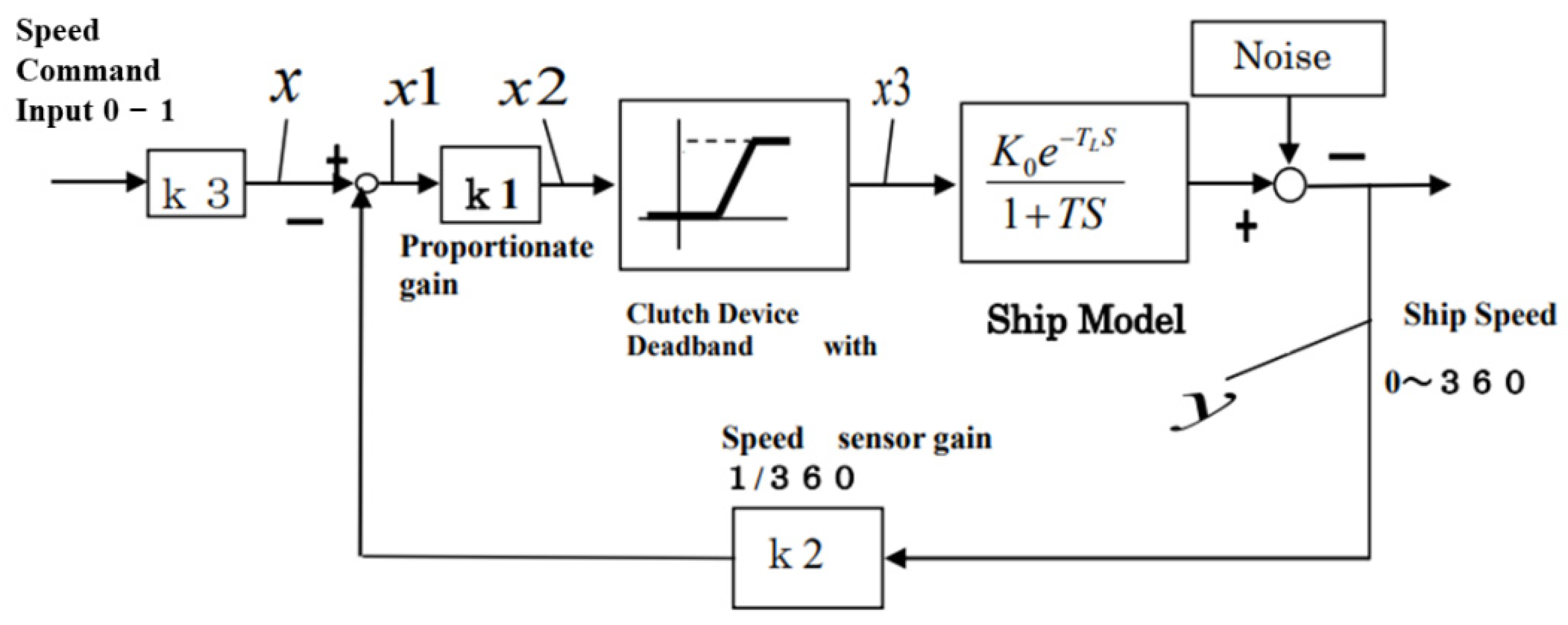
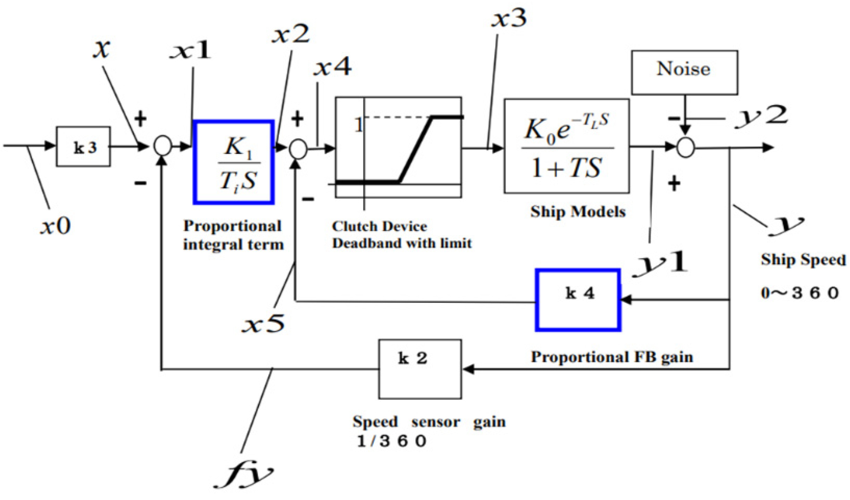
3.1. Control Modeling

The model was created based on the experimental results of the speed step response of a ship in open loop. Since no oscillation was observed, the model was approximated by a first-order delay plus wasted time. The model is shown in Equation (1), where T_L = wasted time, T = time constant, and k₀ = proportional gain.

$$G\left(s\right)=\frac{k_0{e}^{-T_{L}S}}{1+TS}$$

(1)

Here, wasted time: TL = 3.5 s, time constant: T = 10 s, and gain to match speed: k₀ = 360.

The screw is not reversed when the ship slows down. When the ship stops, the input is the same as zero, and the model is almost the same as when stepping up. Figure 2 shows a schematic of the inputs and process.

f is the propulsive force, c is the damper coefficient, m is the mass, and x is the displacement of the ship, using the general equation in (2) (mass–damper system).

$$f=m\stackrel{··}{x}+c\stackrel{·}{x}$$

(2)

Here, input is f, and output is x,

$$F\left(s\right)=m{S}^{2}X\left(s\right)+CSX\left(s\right)$$

(3)

$$F\left(s\right)=X\left(s\right)\{m{S}^2+CS\}$$

(4)

$$G\left(s\right)=\frac{X\left(s\right)}{F\left(s\right)}=\frac{1}{m{S}^2+CS}$$

(5)

Equation (3) is the Laplace transform, Equation (4) is summarized by X(s), and Equation (5) is the transfer function by output/input. The model was then compared with data collected in an open loop with a ramped clutch signal to verify the model. Since the clutch has a deadband (no connection at first), the model includes a signal that takes the deadband into account.

3.2. Various Control Methods (Proportional Control)

Generally, in proportional control, the amount of operation is adjusted gradually as a magnitude proportional to the difference between the target value and the current location. The results of the simulation based on the created model are shown below. A block diagram is shown in Figure 3. The adjustable terms are k1 (proportional gain), k2 (sensor gain), and k3 (input gain).

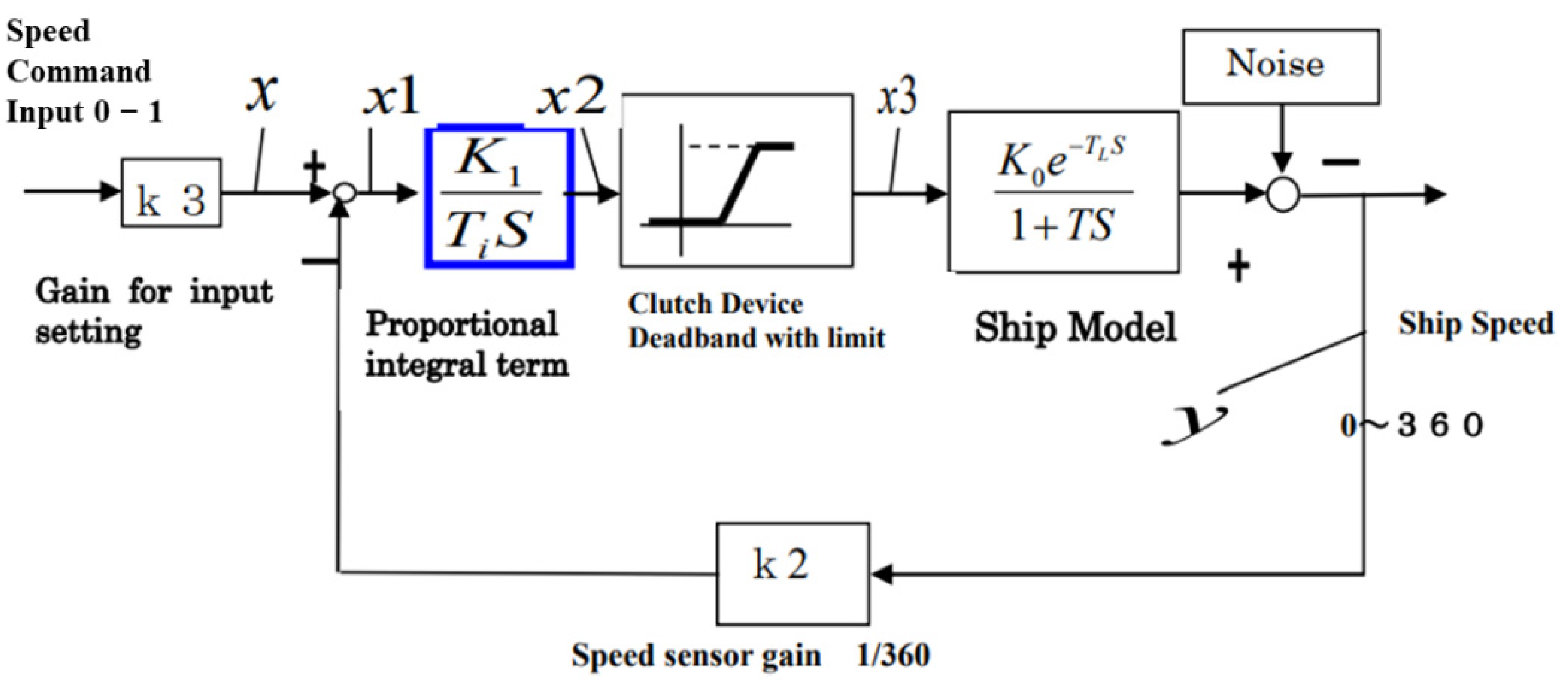
3.3. Various Control Methods (Proportional–Integral (PI) Control)

In general, PI control adds integral control to proportional control to remove residual deviations that cannot be controlled by proportional control. Figure 4 shows a block diagram. The integral is added to the proportional gain in PI control. The terms that can be adjusted are the integral time Ti and the proportional fraction k. The terms that can be adjusted are the integration time Ti and the proportional factor k1.

3.4. Various Control Methods (I-P control, 2-DOF PI Control)

In general, the response speed and overshoot are considered easier to adjust for PI control, because the waveform changes at a constant rate during adjustment, as opposed to PI control. In conclusion, it is easy to adjust and tolerant to disturbances. Figure 5 shows a block diagram of the I-P control system, which has an additional output feedback of k4 compared to PI. In general, this control system is easy to adjust and tolerant of external disturbances.

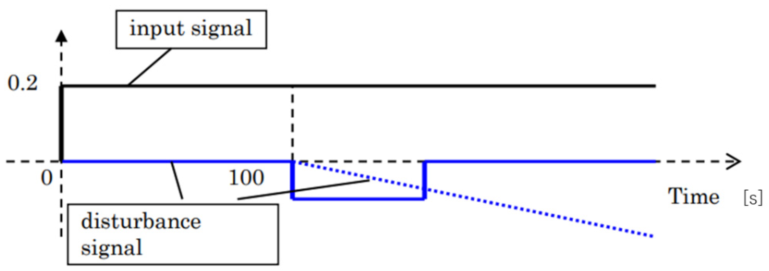
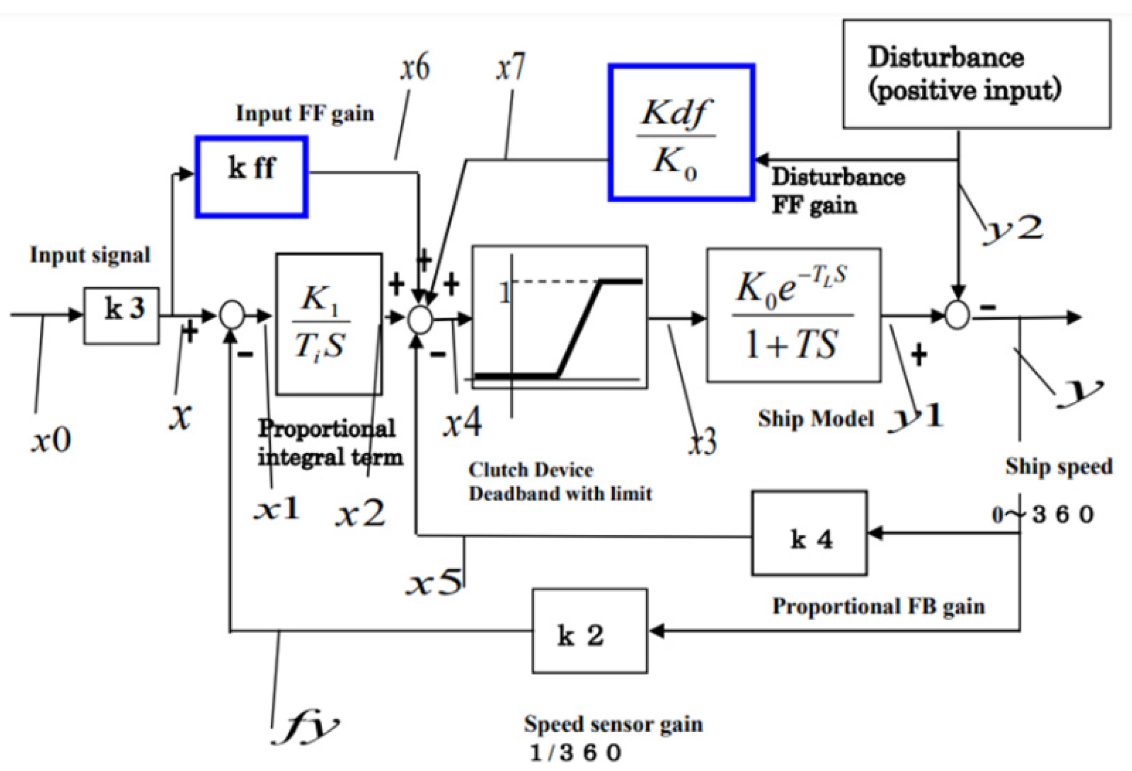
3.5. Methods for Studying the Effects of Disturbances

A disturbance was applied to the I-P control system planned for use in this study, and the response was observed. Continuous steps, step ups and downs of a fixed duration, and ramp disturbances were generated and input to the system. To improve the response to the disturbances, the following two conditions were used.

(1) A feedforward term of the input signal was added.

(2) A feedforward term for the disturbance signal was added.

The input signal was set to 0.2 to account for tidal currents. After 100 s, when the speed control had stabilized, the disturbance was input. A summary of the observed response of the I-P control system under disturbance input is shown in Figure 6. Figure 6 is a time-domain graph.

(1) Addition of input signal feedforward term

Feedforward is generally used to speed up the rise response. To compensate for the slowdown in the case of a disturbance, a feedforward (FF) term (Kff) of the input signal was added to I-P to increase the response speed. A block diagram is shown in Figure 7.

(2) Addition of a disturbance signal feedforward term

Figure 8 shows a block diagram of the disturbance FF for the purpose of improving the response to disturbance input.

3.6. Software and Experiments

The actual data are obtained by a speedometer attached to a fish finder. The software for simulation is EQUATRAN-G (Ver. 3.1.3).

4. Results

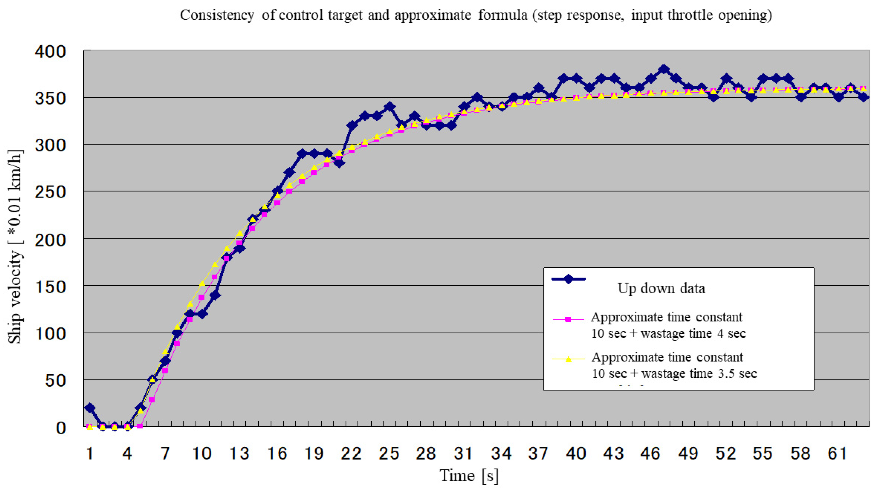
4.1. Model to Be Controlled

Figure 9 shows the results of the comparison with the step-up model. When the time constant is 10 s and the wasted time 3.5 s is compared with the wasted time 4.0 s, the wasted time 3.5 s seems to be more consistent with the model. Figure 10 shows the results of step descent. The dark blue graph shows the measured data, yellow shows the measured data plus 1 s, and pink shows the simulated data. In addition to the fact that it was found that the rise model can approximate the fall data as well, and given that the rise model is used more often in real data, the rise model is utilized in this paper. Figure 11 shows the results of the simulation comparison of ramp inputs. Dark blue represents the simulation results, pink represents the real data, and yellow represents the DA values. Light blue shows the values when the screw is reversed.

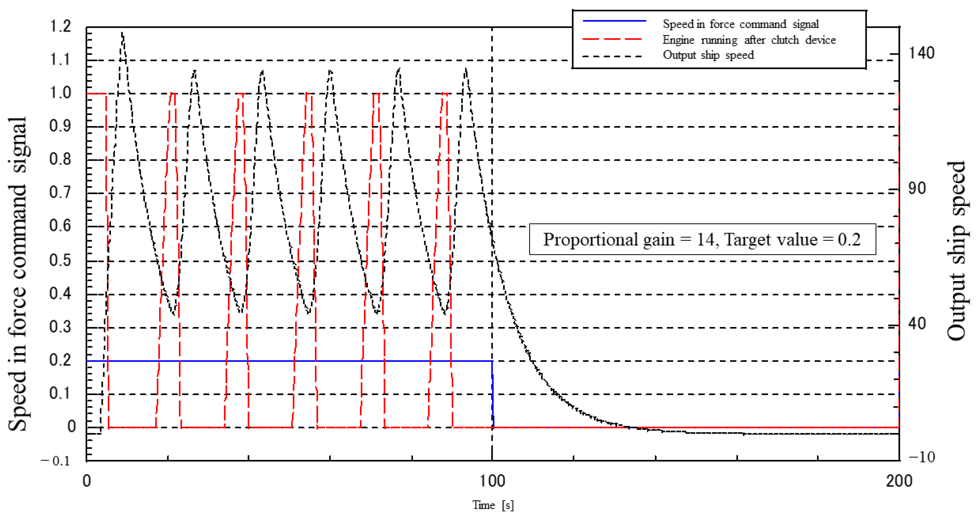
4.2. Various Control Results (Proportional Control)

The clutch operates according to the signal from the D/A converter. The DA value ranges from 110 (fast) to 225 (slow), and the clutch does not connect from 225 to 195. The relationship is shown in Figure 12.

Figure 13 shows the step input results when the proportional gain is increased by a factor of 20 and the input is set from 0 to 1. 150 s input is set back to 0. The clutch device takes a long time to saturate to 1, and the vibration does not subside.

Figure 14 shows a target value of 0.2, but the vibration does not subside.

Figure 15 is stable, but the proportional gain is low (=2) and the speed does not reach the target value (360).

Figure 16 shows the results with and without the blind zone at the clutch. Although the vibration is smaller, there is no significant difference in the response waveform. This is because there is no delay in the proportional response. Figure 16 indicates that proportional control alone would be difficult to achieve for this subject.

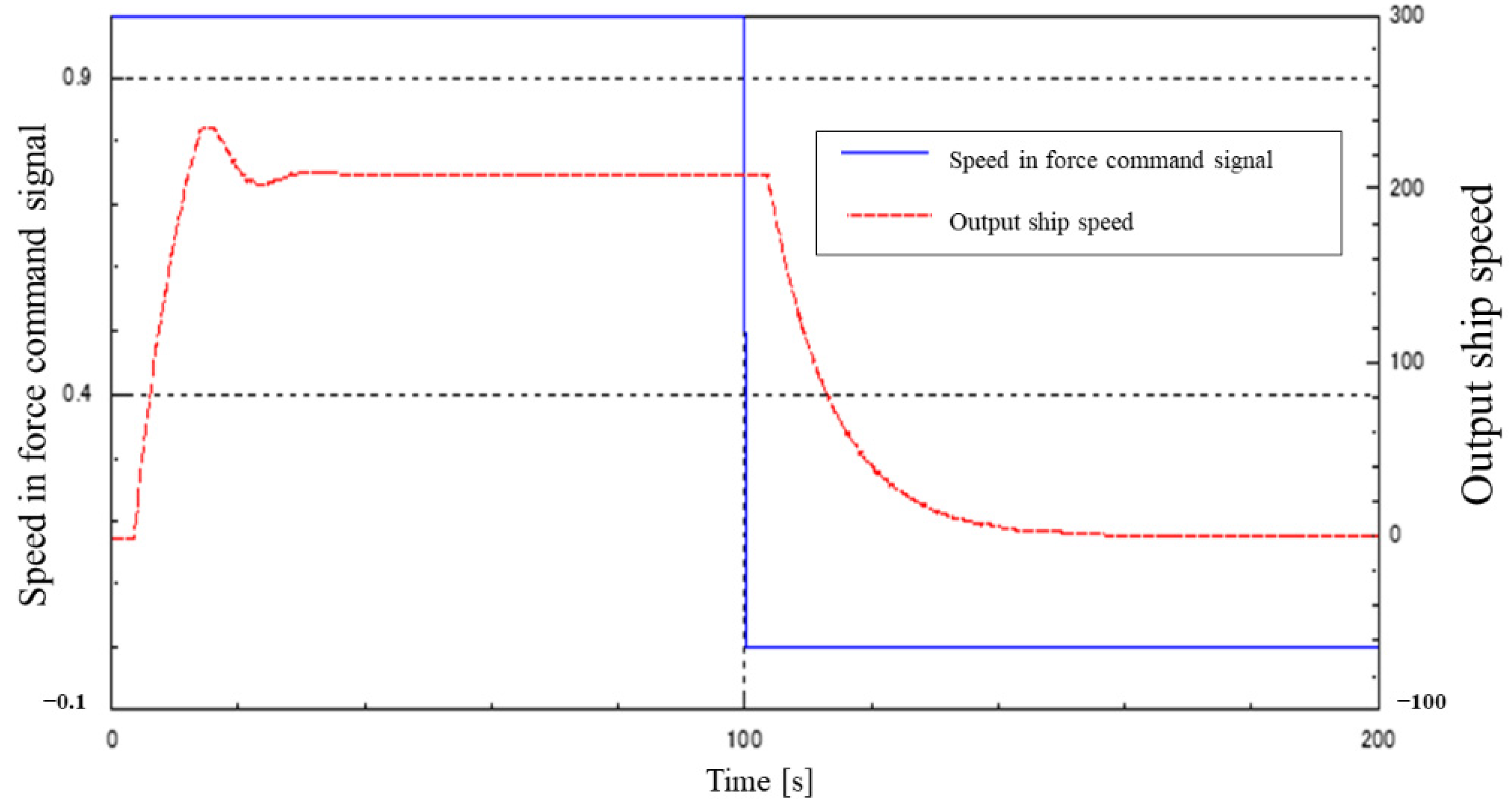
4.3. Various Control Results (Proportional–Integral (PI) Control)

Figure 17 shows an example of step response with Ti = 15 s, target value 0.2 input, and K1 = 1.0. Although the system is stabilized, the response is slow. However, because integration is included, the deviation is zero.

Figure 18 shows the step response waveform of the clutch with a dead zone at the same set value as in Figure 17, but the time to reach the target value is faster than in Figure 17. There is no significant difference in the control waveforms.

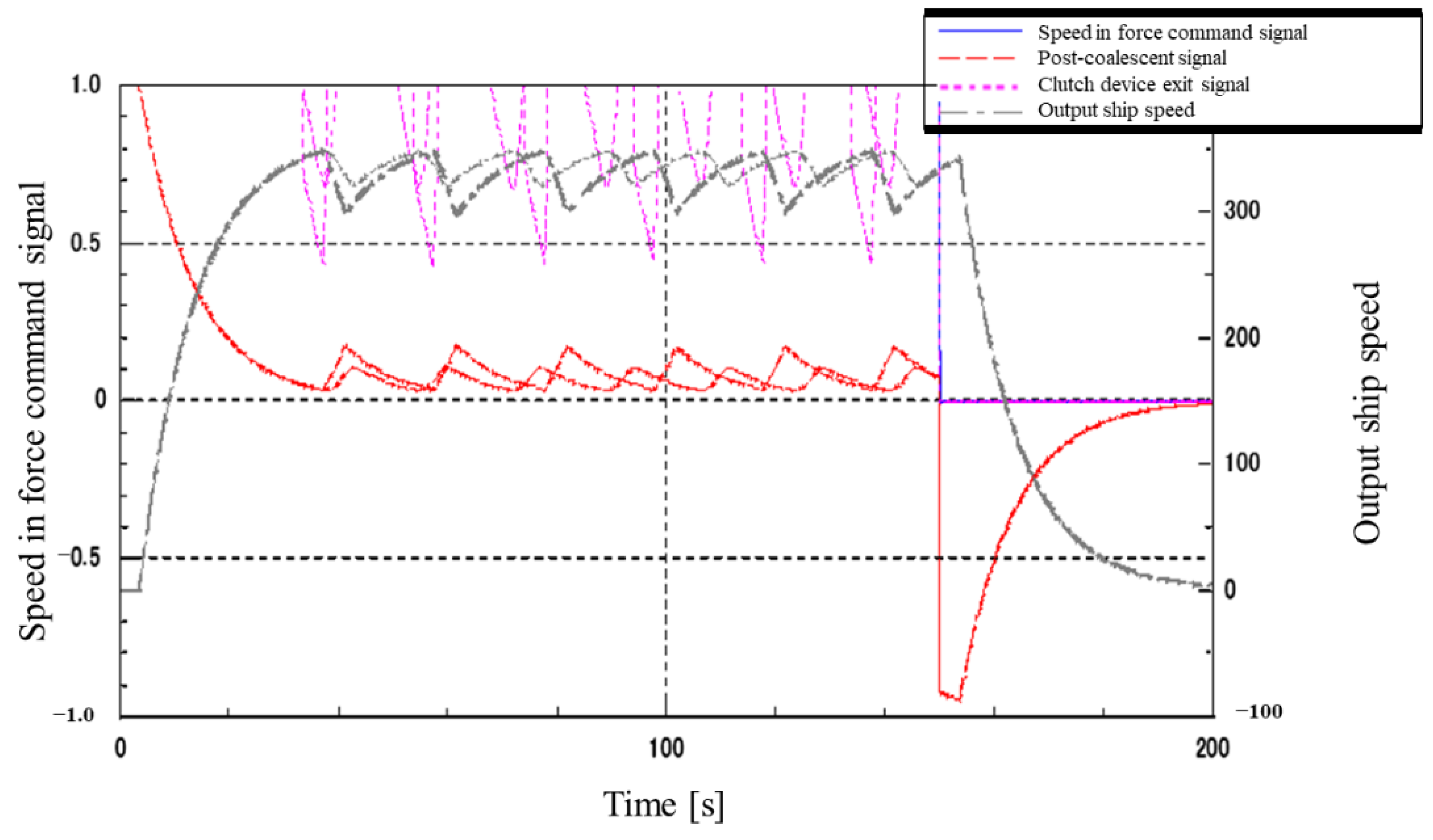
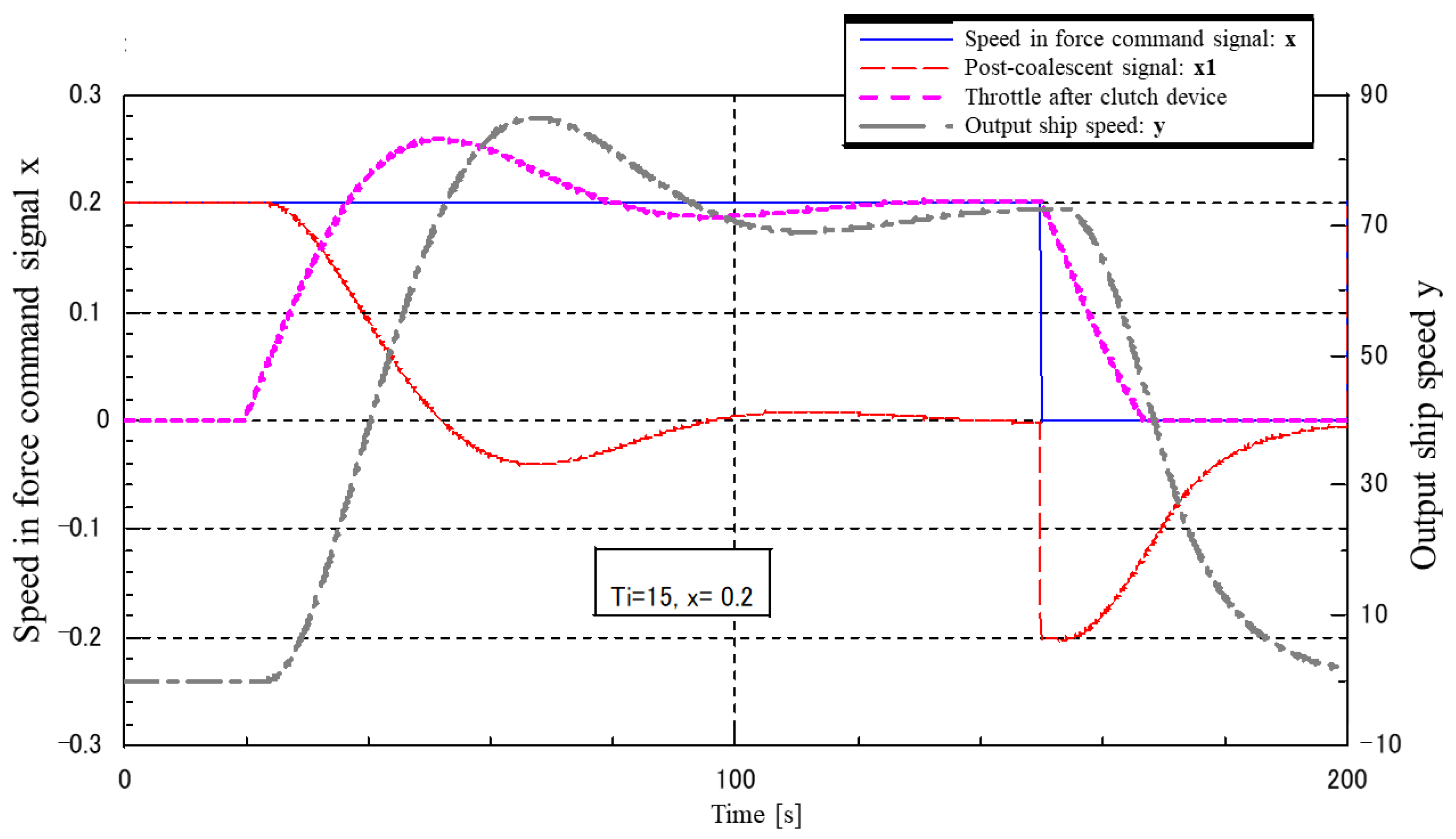
4.4. Various Control Results (I-P Control, 2-DOF PI Control)

Figure 19 shows an example of step response with the same Ti and K1 as in Figure 17 of the PI control, and the superiority of stability compared to the PI control is observed.

Figure 20 shows an example of step response with I-P adjustment, and it can be observed that both response speed and stability are greatly improved compared to PI control.

Figure 21 shows the same adjustment as in Figure 20, but without the blind zone and with the blind zone superimposed. The response is improved by removing the dead zone.

Figure 22 shows the result of adjusting the response of the I-P control system to the point where it is on the verge of oscillation.

4.5. Results of the Effects of Disturbances

Figure 23 and Figure 24 show the results of including a step-like disturbance (no lowering) of varying magnitude in the I-P control system. In the model, 0.2 times the maximum speed was continuously input as the target value, and disturbances of 0.05 and 0.1 times the maximum speed of the ship were input after 100 s. The disturbance was applied 100 s later. After the disturbance, the speed dropped and the waveform was disturbed, but it was observed that the speed returned to the target value.

Figure 25 shows the response waveform when a disturbance of the same magnitude as the input signal is applied. The speed is restored as before, but there is a time when the speed becomes zero.

Figure 26 shows the results of inputting a step disturbance (with lowering) at the same speed as the ship, but only between 80 s and 100 s. When the disturbance is large, there are times when the speed drops to zero even when the disturbance acts for 20 s. The waveform is also greatly disturbed.

(1) Addition of input signal feedforward term

Figure 27 shows a comparison of a disturbance input waveform (Kff = 2.5) with and without FF. The input FF speeds up the response at the rise of the input signal. However, the speed of the waveform is reduced to 0 when the FF is applied, and no difference can be seen in the waveform after that. Therefore, the effectiveness of this method against disturbances could not be confirmed.

(2) Addition of disturbance signal feedforward term

Figure 28 shows the superimposed waveforms with and without the disturbance FF. With the disturbance FF, the clutch signal reaches its maximum value at a high speed because the disturbance signal is fed directly into the clutch. However, there is no change in the time when the ship comes to a stop, perhaps due to wasted time, and the subsequent waveforms oscillate more significantly with FF. The above results show that the addition of the disturbance FF did not have any effect on the disturbance.

4.6. Summary of Results

Figure 13, Figure 14, Figure 15, Figure 16, Figure 17, Figure 18, Figure 19, Figure 20, Figure 21 and Figure 22 showed that I-P control can increase both responsiveness and stability compared to proportional and PI control. Figure 23, Figure 24, Figure 25, Figure 26, Figure 27 and Figure 28 also show that feedforward was tried to reduce the effect of disturbances, which resulted in increased responsiveness.

5. Discussion

In this study, with proportional control alone, oscillations were likely to occur, and if oscillations were not allowed to occur, steady-state deviations occurred. When integrals were added, the response became slower. When I-P was added, the steady-state deviation was eliminated, and the speed could be increased.

Therefore, it is appropriate to use an I-P control system (2-DOF PI control) as the control method for constant ship speed control. To increase the response speed, it is also effective to use feedforward input and to eliminate the dead zone of the clutch device. Increasing engine power increases the adjustment range of the control system.

5.1. The Model to Be Controlled

The ship model used in this study can be approximated to some extent by the first-order delay and wasted time. Comparisons with real data on a ramped input signal yielded good results. The rise and fall of the step response can also be described by a single model.

5.2. Various Control Methods

(i) Proportional control

In the fishing vessels for which experimental data were taken, it is difficult to perform automatic control using only a proportional control system. The steady-state deviation becomes too large for a gain that can ensure stability. In addition, even if the engine output is increased relative to the ship’s clutch or the screw is reversed, the proportional gain cannot be increased.

(ii) PI control

Integral and proportional (PI control system) can be used to stabilize the system, but it is difficult to achieve a fast response while maintaining stability. For stability, it is important to control the clutch so that it does not saturate (see results below). Because of the integration, the steady-state position deviation from the input command can be set to zero.

(iii) 2-DOF PI control system (I-P control system)

This control system has good stability and fast response. This is the best method among the control systems tested in this study.

(iv) I-P control system + input signal feedforward

A faster response to input signals than I-P was possible.

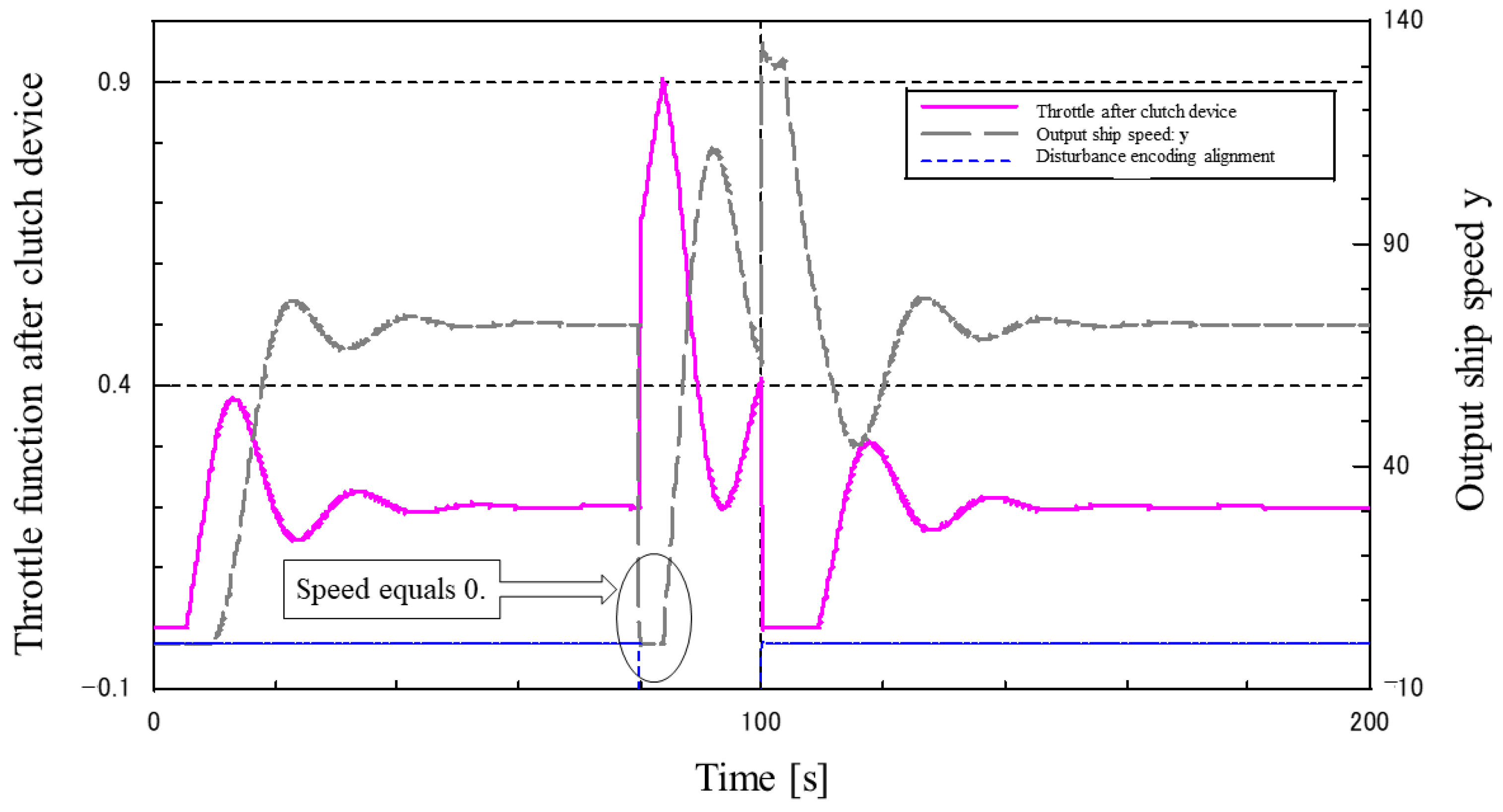
5.3. Disturbance Input to I-P Control System

(i) When a step disturbance (in the direction of stopping the ship) is applied, the waveform is disturbed immediately after the disturbance is applied but returns to a steady state after a certain period. This is true whether the disturbance is applied continuously or discretely. However, when a disturbance of the same magnitude as the input is applied, there will be a time when the ship’s speed is zero. Additionally, due to the effect of integration, the steady-state position deviation due to the disturbance becomes zero.

(ii) To speed up the response after a step disturbance, the disturbance signal was input to the system in a feedforward manner, but no effect was observed. (Since the actual disturbance cannot be measured directly, a model was built into the controller and the results were calculated using calculations with the actual data.) Similarly, no effect was observed in the feedforwarding of input signals. This was thought to be since the ship’s speed was output after a certain period had elapsed after the screw rotated, resulting in a waste of time.

(iii) The perfect response to step disturbances is to eliminate the wasted time and to predict the disturbance, which is difficult to achieve. However, in actual sea areas, wave shapes are more complex, and it is not considered necessary to respond perfectly to step-like disturbances. In addition, for ramp-like disturbance inputs, the steady-state speed deviation cannot be set to zero because I-P has only one integral element and is of type 1. To set the steady-state speed deviation to 0, an attempt was made to control the system with a type 2 system, but it could not be stabilized.

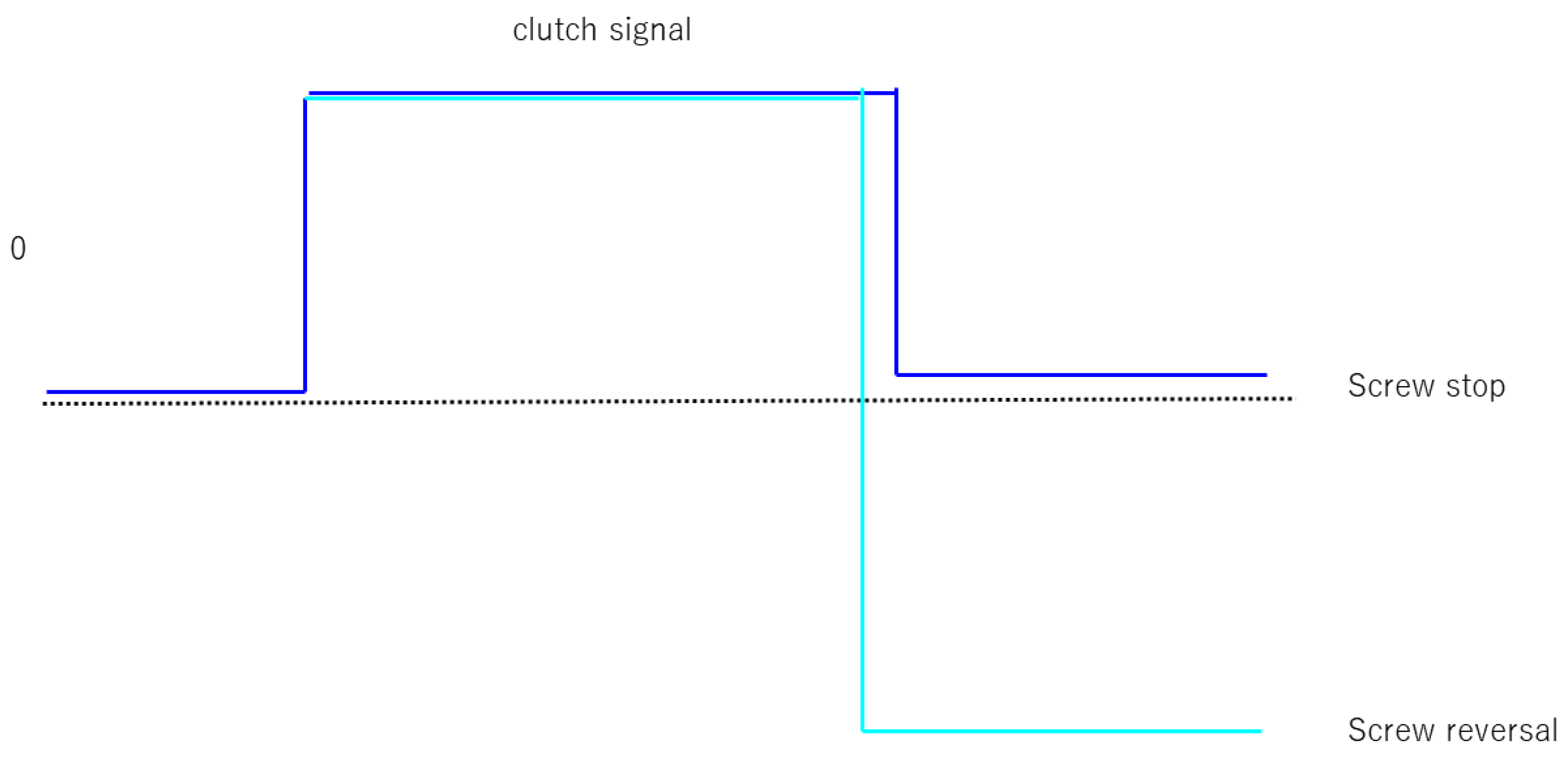
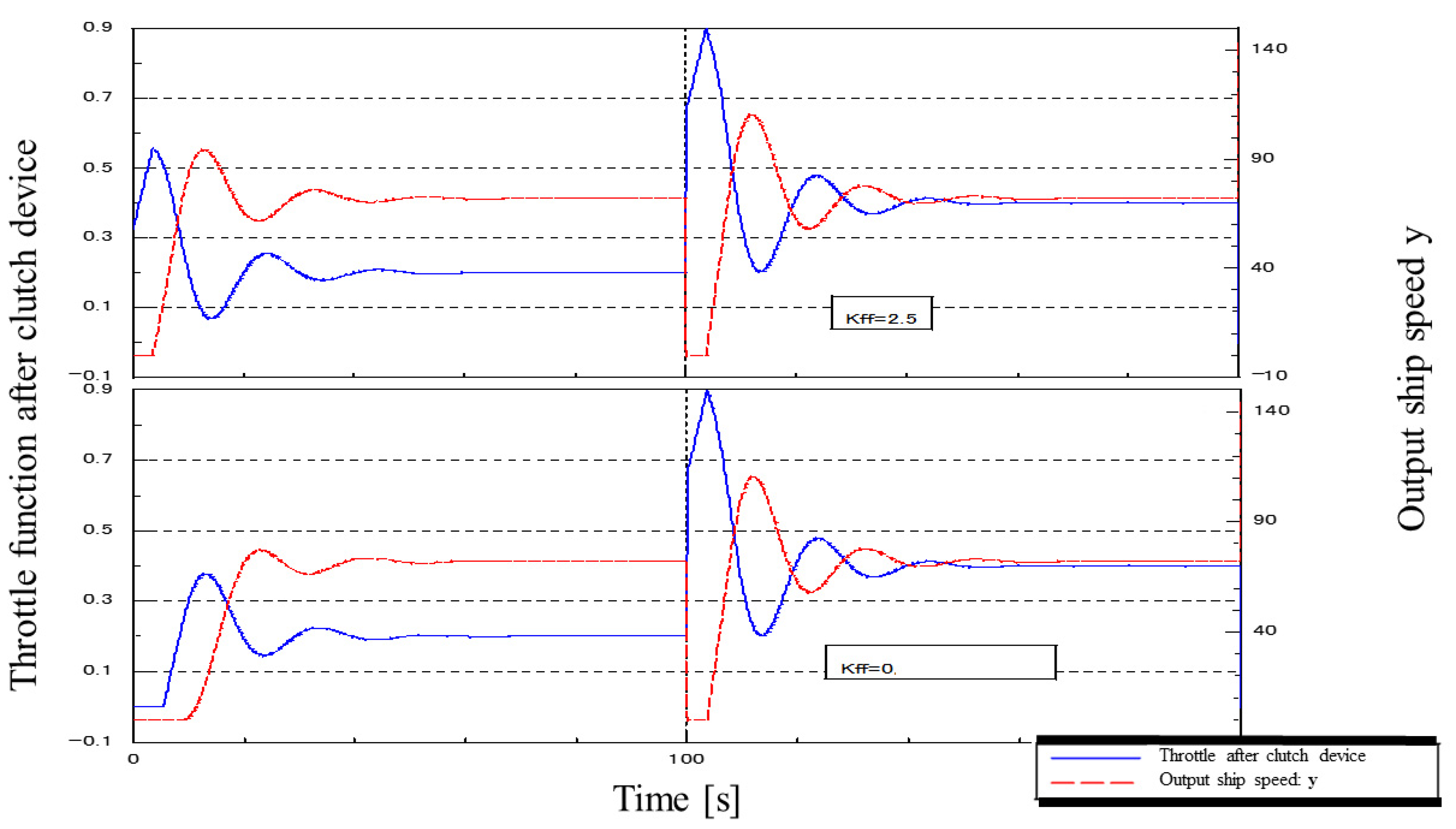
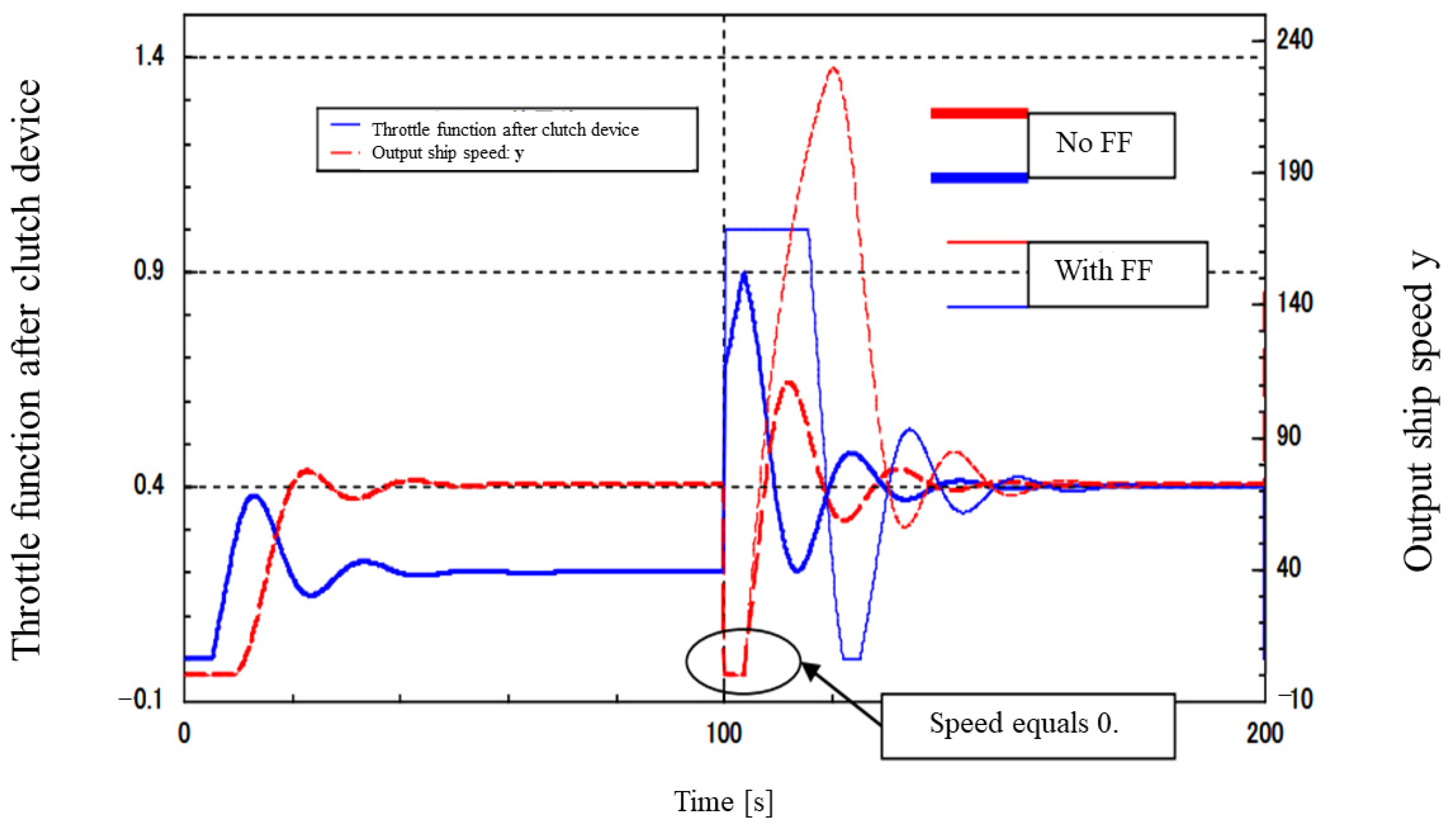
5.4. Dead Zone of the Clutch

Eliminating the blind zone in the clutch device speeds up the response but does not have much effect on controllability. Therefore, it could be inferred that it is not necessary to place an economic burden on the clutch device, but rather it is important to equip the engine with high response.

6. Conclusions

This paper focused on the automated navigation of trawl fishing methods in a largehead hairtail fishery. An optimal speed controller for the automated trawl fishing method was developed and modeled. Next, the optimal automatic control system was identified using simulation (SLAFT) among proportional control, PI control, I-P control, and I-P + feedforward control. Finally, various disturbances were input to the control method considered to be the most suitable among these, and their effects were observed. Theoretically, PI control is possible to obtain up to a range, but in practice, because of incompatibility due to vibration and response speed delays, I-P control, which is easy to adjust by varying the integral and proportional feedback terms, was adopted. After trial and error and considering the degree of vibration that could not be resolved by simulation, we concluded that I-P control is optimal. Trial runs on actual vessels also yielded good results.

The ship model could be approximated to some extent by first-order delay and wasted time. Comparisons with real data were made with ramped input signals, and good results were obtained. The fact that the rise and fall during the step response can also be described by a single model suggests that the model is versatile. The study revealed the best stability and, at the same time, the fastest response when using a 2-DOF PI control system (I-P control system). In addition, it is inferred that the system will be able to respond to step-like disturbances once wave prediction becomes possible. Through this research, it will be possible to develop methods in fisheries that can efficiently exploit the global aquatic biodiversity and respond to human demand for fish and shellfish. Through the progressive integration of information technology, data science, and artificial intelligence with fisheries and aquaculture methods, the authors sincerely hope that SLAFT will increasingly contribute to the conservation of the global environment and ecosystems.

References

1. Gladju, J.; Kamalam, B.S.; Kanagaraj, A. Applications of data mining and machine learning framework in aquaculture and fisheries: A review. Smart Agric. Technol. 2022, 2, 100061. [Google Scholar] [CrossRef]
2. Glaviano, F.; Esposito, R.; Cosmo, A.D.; Esposito, F.; Gerevini, L.; Ria, A.; Molinara, M.; Bruschi, P.; Costantini, M.; Zupo, V. Management and Sustainable Exploitation of Marine Environments through Smart Monitoring and Automation. J. Mar. Sci. Eng. 2022, 10, 297. [Google Scholar] [CrossRef]
3. Al-Absi, M.A.; Kamolov, A.; Al-Absi, A.A.; Sain, M.; Lee, H.J. IoT Technology with Marine Environment Protection and Monitoring. In International Conference on Smart Computing and Cyber Security; Springer: Singapore, 2021; pp. 81–89. [Google Scholar]
4. Liu, J.; Aydin, M.; Akyuz, E.; Arslan, O.; Uflaz, E.; Kurt, R.E.; Turan, O. Prediction of human–machine interface (HMI) operational errors for maritime autonomous surface ships (MASS). J. Mar. Sci. Technol. 2022, 27, 293–306. [Google Scholar] [CrossRef]
5. Liu, C.; Chu, X.; Wu, W.; Li, S.; He, Z.; Zheng, M.; Zhou, H.; Li, Z. Human–machine cooperation research for navigation of maritime autonomous surface ships: A review and consideration. Ocean Eng. 2022, 246, 110555. [Google Scholar] [CrossRef]
6. Zinchenko, S.; Mateichuk, V.; Nosov, P.; Popovych, I.; Solovey, O.; Mamenko, P.; Grosheva, O. Use of simulator equipment for the development and testing of vessel control systems. Sci. J. Riga Tech. Univ.-Electr. Control. Commun. Eng. 2020, 16, 58–64. [Google Scholar] [CrossRef]
7. Vander Hook, J.; Seto, W.; Nguyen, V.; Hasnain, Z.; Gallagher, L.; Halpin-Chan, T.; Varahamurthy, V.; Angulo, M. Autonomous swarms of high speed maneuvering surface vessels for the central test evaluation improvement program. Unmanned Syst. Technol. XXI 2019, 11021, 140–149. [Google Scholar]
8. Erol, E.; Cansoy, C.E.; Aybar, O.Ö. Assessment of the impact of fouling on vessel energy efficiency by analyzing ship automation data. Appl. Ocean Res. 2020, 105, 102418. [Google Scholar] [CrossRef]
9. Amoroso, R.O.; Pitcher, C.R.; Rijnsdorp, A.D.; McConnaughey, R.A.; Parma, A.M.; Suuronen, P.; Eigaard, O.R.; Bastardie, F.; Hintzen, N.T.; Althaus, F.; et al. Bottom trawl fishing footprints on the world’s continental shelves. Proc. Natl. Acad. Sci. USA 2018, 115, E10275–E10282. [Google Scholar] [CrossRef] [PubMed]
10. Watling, W.; Norse, E.A. Disturbance of the seabed by mobile fishing gear: A comparison to forest clear cutting. Conserv. Biol. 1998, 12, 1180–1197. [Google Scholar] [CrossRef]
11. NRC. Effects of Trawling and Dredging on Seafloor Habitat; National Academy Press: Washington, DC, USA, 2002. [Google Scholar]
12. Piet, G.J.; Hintzen, N.T. Indicators of fishing pressure and seabed integrity. ICES J. Mar. Sci. 2012, 69, 1850–1858. [Google Scholar] [CrossRef]
13. Gerritsen, H.D.; Minto, C.; Lordan, C. How much of the seabed is impacted by mobile fishing gear? Absolute estimates from Vessel Monitoring System (VMS) point data. ICES J. Mar. Sci. 2013, 70, 523–531. [Google Scholar] [CrossRef]
14. Kaiser, M.J.; Collie, J.S.; Hall, S.J.; Jennings, S.; Poiner, I.R. Modification of marine habitats by trawling activities: Prognosis and solutions. Fish Fish. 2002, 3, 114–136. [Google Scholar] [CrossRef]
15. Fock, H. Fisheries in the context of marine spatial planning: Defining principal areas for fisheries in the German EEZ. Mar. Policy 2008, 32, 728–739. [Google Scholar] [CrossRef]
16. Churchill, J.H. The effect of commercial trawling on sediment resuspension and transport over the Middle Atlantic Bight continental shelf. Cont. Shelf Res. 1989, 9, 841–864. [Google Scholar] [CrossRef]
17. Bastardie, F.; Angelini, S.; Bolognini, L.; Fuga, F.; Manfredi, C.; Martinelli, M.; Nielsen, J.R.; Santojanni, A.; Scarcella, G.; Grati, F. Spatial planning for fisheries in the Northern Adriatic: Working toward viable and sustainable fishing. Ecosphere 2017, 8, e01696. [Google Scholar] [CrossRef] [Green Version]
Figure 1. An overview of trawl fishery.
Automation 03 00027 g001
Figure 2. Schematic of the inputs and process.
Automation 03 00027 g002
Figure 3. Proportional control block diagram.
Automation 03 00027 g003
Figure 4. Proportional–integral (PI) control block diagram.
Automation 03 00027 g004
Figure 5. I-P control system block diagram.
Automation 03 00027 g005
Figure 6. Summary of observed response of I-P control system under disturbance input.
Automation 03 00027 g006
Figure 7. I-P control system + input feedforward.
Automation 03 00027 g007
Figure 8. I-P control system + disturbance feedforward input.
Automation 03 00027 g008
Figure 9. Comparison of model and real data (at startup).
Automation 03 00027 g009
Figure 10. Comparison of model and real data (at falling edge).
Automation 03 00027 g010
Figure 11. Ramped Input Simulation Comparison.
Automation 03 00027 g011
Figure 12. The relationship of input and output.
Automation 03 00027 g012
Figure 13. Proportional control result (proportional gain 20, input 0–1).
Automation 03 00027 g013
Figure 14. Proportional control result (proportional gain 14, input 0–0.2).
Automation 03 00027 g014
Figure 15. Proportional control result (proportional gain 2, input 0–1).
Automation 03 00027 g015
Figure 16. Comparison of clutch with and without dead zone.
Automation 03 00027 g016
Figure 17. Proportional–integral (PI) step response waveform Ti = 15 s, K1 = 1.0, target value 0.2, with dead zone.
Automation 03 00027 g017
Figure 18. Proportional–integral (PI) step response waveforms with the same settings as Figure 17, but with a clutch deadband.
Automation 03 00027 g018
Figure 19. I-P control step response waveform. (Ti = 15 s, K1 = 1.0, target value 0.2, K4 = 0.5 × K2 with blind zone, with the same Ti and K1 settings as in Figure 17.)
Automation 03 00027 g019
Figure 20. I-P control step response waveform (Ti = 4 s, K1 = 1.0, target value 0.2, K4 = K2 × 1.7 with dead zone).
Automation 03 00027 g020
Figure 21. I-P control step response waveforms (Overlaid with and without dead zone, Ti = 4 s, K1 = 1.0, target value 0.2, K4 = K2 × 1.7).
Automation 03 00027 g021
Figure 22. I-P control step response waveform. (Response increased to the point of oscillation, Ti = 3 s, K1 = 1.0, target value 0.2, K4 = K2 × 2.3, with dead zone.)
Automation 03 00027 g022
Figure 23. I-P control step + disturbance response waveform (Ti = 4.1 s, K1 = 1.0, target value 0.2, K4 = K2 × 1.7, with dead zone, disturbance = ship max speed × 0.05).
Automation 03 00027 g023
Figure 24. I-P control step + disturbance response waveform. (Ti = 4.1 s, K1 = 1.0, target value 0.2, K4 = K2 × 1.7, with dead zone, disturbance = ship max speed × 0.1.)
Automation 03 00027 g024
Figure 25. I-P control step + disturbance response waveform. (Ti = 4.1 s, K1 = 1.0, target value 0.2, K4 = K2 × 1.7, with dead zone, disturbance = ship max speed × 0.2.)
Automation 03 00027 g025
Figure 26. I-P control step + disturbance response waveform. (Ti = 4.1 s, K1 = 1.0, target value 0.2, K4 = K2 × 1.7, with deadband, disturbance = ship max speed × 0.2, 20 s.)
Automation 03 00027 g026
Figure 27. (Up) I-P control + input FF, Kff =2.5 (Down) step + disturbance response waveform, Kff = 0 (I-P control, step + disturbance response waveform, Ti = 4.1 s, K1 = 1.0, target value 0.2, K4 = K2 × 1.7, with dead zone, disturbance = ship max speed × 0.2).
Automation 03 00027 g027
Figure 28. I-P control, Overlay with and without disturbance FF, Example of step + disturbance continuous response waveform (Ti = 4.1 s, K1 = 1.0, target value 0.2, K4 = K2 × 1.7, with dead zone, disturbance = ship max speed × 0.2, Kff = 0, Kdf = 7.0).
Automation 03 00027 g028
Publisher’s Note: MDPI stays neutral with regard to jurisdictional claims in published maps and institutional affiliations.