Modeling and Control of Satellite Formations: A Survey

Abstract

This survey deals with the problem of the group motion of spacecraft, which is rapidly developing and relevant for many applications, in terms of developing the onboard control algorithms to ensure the fulfillment of a given mission. The paper provides a comprehensive overview of spacecraft formation flight control. The bibliography is divided into three main sections: the multiple-input–multiple-output approach, in which the formation is treated as a single entity with multiple inputs and multiple outputs; the leader–follower formation, in which individual spacecraft controllers are linked hierarchically; and a virtual structure formation, in which spacecraft are treated as rigid bodies embedded in a common virtual rigid body. This survey expands a 2004 survey and updates it with recent results.

1. Introduction

Satellite formations find many applications in the various fields, including Earth surveillance, geodesy, astronomy, space exploration, etc. Following [1], the satellite formation flight (SFF) can be defined as the movement of a group of more than one spacecraft whose dynamic states are coupled by a common control law (see also [2]). At the same time, at least one satellite (formation agent) must track the desired state relative to another agent, and the tracking law must minimally depend on the state of this other agent. For example, even if specific relative positions are actively maintained, the Global Positioning System (GPS) satellites form a formation because only the position and speed of an individual satellite need to be used to correct their orbital motion.

Let us present some examples. The distributed space missions with application to Earth observation with special emphasis on radar payloads are presented in [3]. Schilling et al. [4] described the distributed satellite system Telematics Int. Mission (TIM), which is a formation of nine cooperating small satellites for photogrammetric Earth observation. TIM’s application scenario focuses on the characterization of ash clouds from volcano eruptions, providing useful information to plan detour maneuvers for airplanes to avoid damage to engines. The CloudCT mission [5] uses a formation of 10 nano-satellites to detect the 3D properties of clouds. CloudCT integrates interdisciplinary synergies from nano-satellite system engineering, cloud modeling, and tomographic imaging to enable a sensor network approach to innovative Earth observation. As Freimann et al. [6] mentioned, nano-satellites offer an affordable way to realize distributed systems for various scientific and commercial applications in the area of Earth observation and global communication services. Freimann et al. [6] presented a contact plan design approach that solves the Medium Access Control (MAC) problem by predicting additive multi-node interference and scheduling interference-free links based on these predictions.

The UWE-program aimed for in-orbit demonstrations of key technologies to enable formations of cooperating distributed spacecraft at the pico-satellite level is presented in [7]. In this program framework, the CubeSat UWE-3 is used for the experiments of evaluation of real-time attitude determination and control. The spacecraft formation consists of a group of satellites performing a single mission, which is usually difficult to accomplish with a single device [8,9,10]. For example, Bik et al. [9] described a joint project between ESA and NASA called the Laser Interferometer Space Antenna (LISA), which will become the first space observatory for gravitational waves. Its main purpose is to detect and observe gravitational waves from massive black holes and binary galaxies in the frequency range ${10}^{-4}$–${10}^{-1}$ Hz. LISA consists of three identical spacecraft located at a distance of $5\times {10}^6$ km from each other in the form of an equilateral triangle. LISA tracks the stretching of space-time caused by gravitational waves by measuring the change in distance between two formation agents using laser interferometry. Three agents will provide independent information about the polarization of the gravitational wave. One shoulder is determined by the distance between the test masses at the ends of each branch of the triangle, which are covered by satellites so that they are not affected by non-gravitational forces. The satellites counteract non-gravitational forces using micro-Newtonian thrusters to follow the trial mass path through what is called drag-free control [11]. Schilling [12] considered technologies for implementing sensor networks in orbit for joint measurements by small satellites weighing several kilograms. It is shown that through sensor data fusion and post-processing, innovative distributed methods of Earth observation can be obtained. In [12], exemplary nano-satellite missions in the field of formations are also outlined. The first demonstration of collision avoidance and orbit control for UWE-4 pico-satellites is presented in Kramer and Schilling [13]. A possible collision with a piece of space debris was avoided by UWE-4 by use of its orbit control capabilities for an evasive maneuver in early July 2020. This maneuver increased the miss distance from 822 m to more than 6000 m. The results, presented in [13] demonstrate perspectives for small spacecraft to comply with regulations on de-orbiting and capabilities for collision avoidance maneuvers. Ref. Mathavaraj and Padhi [14] used the optimal and adaptive control techniques to develop the satellite formation flying-high precision guidance.

The mentioned examples are related to the SFF missions and the formation flying guidance (FFG), which is considered as the generation of the reference trajectories used as an input for a formation agent’s relative state tracking control law. The examples mentioned are related to the SFF missions and the formation flying guidance (FFG), which is considered as the generation of any reference trajectories used as an input for a formation agents’ relative state tracking control law [1]. A detailed and informative review of the results on the control of spacecraft formations can also be found in the monograph [15], which presents fundamental problems and approaches related to group flights of spacecraft, provides information on the dynamics of satellite motion, considers methods of static optimization, feedback control, and filtration, the nonlinear models of the relative spacecraft motion, including the rendezvous of satellites, orbital perturbations and methods for their effect mitigating, as well as the methods for groups of spacecraft control algorithms development.

To implement the given navigation laws by individual agents of the group, control algorithms are developed—both local control algorithms for each satellite separately, and algorithms based on the receipt by individual agents of data on the state (e.g., positions and velocities) of other satellites.

This paper provides a comprehensive overview of spacecraft formation flight control (SFFC), covering design methods and stability results analysis for these coupled state control laws. Since the SFFC architecture defines a general approach to the development of a particular SFFC algorithm, it is reasonable to organize publications according to the formation architecture. Therefore, following the lines of the 2004 review on the subject [1], in the present paper, the SFFC literature is divided into three main types: Multiple-Input–Multiple-Output (MIMO), in which the formation is treated as a single entity with multiple inputs and multiple outputs; the leader–follower (LF) formation, in which individual spacecraft controllers are linked hierarchically; and a virtual framework as the virtual structure (VS) formation, in which spacecraft are treated as rigid bodies embedded in a common virtual rigid body, and the master/slave configuration. This survey is aimed to expand [1] and present modern results of recent years. When picking up papers for reviewing, the authors have largely been guided by the influence of the papers on other publications in the field. For example, works [16,17,18] by the time of the review submission received 237, 193, 156 citations, respectively, in the database Scopus. In addition, the selection of material in this work was undoubtedly influenced by the scientific interests of the authors, who apologize in advance to colleagues whose contributions were outside the main focus of this review.

The rest of the paper is organized as follows. Section 2 deals with the MIMO formation architecture. The circle formation is described in Section 3, whilst Section 4 is devoted to leader–follower architecture. Concluding remarks of Section 5 finalize the paper. In general, the references inside each Section are given in chronological order.

2. Multiple-Input–Multiple-Output Formation Architecture

Vassar and Sherwoodt [18] developed a feedback controller to maintain a movement of a swarm of satellites using the calculated optimal trajectory. Chemical thrusters are used for the slave satellite as the actuators. The situation is considered when two satellites fly at a distance of 700 m from the geophysical orbit. The results of [18] show that movement in the swarm can be maintained at a distance of 21 m of satellites from each other.

Ulybyshev [19] studied keeping the satellite formation in near-circular orbits. The tangential maneuvers of a group of satellites are determined by continuous relative motion equations. During the entire movement, the satellites move relative to each other, and these movements are presented in the form of a graph. In [19], $(2N-1)$ linearized equations, where N is the total number of satellites are used. A linear-quadratic controller has been developed to control satellite formation. An analytical solution of linear-quadratic equations for the formation of two satellites is found. The simulation results for low Earth orbits (LEO) are presented where atmospheric drag is taken into account.

Inalhan et al. [20] focused on the planning of missions that provide the necessary conditions for the initialization of a periodic formation of a satellite constellation that provides a good distributed image of the Earth, for example, using synthetic aperture radar. These passive apertures were previously designed using the closed form solution provided by the Hill equations (see [21,22]), also known as the Clohessy–Wiltshire equations [23], which are linearized with respect to the near-circular reference orbit. A study was carried out to develop apertures that are insensitive to differential noise $J_2$ (the second zonal harmonic $J_2$ characterizes the polar compression). Based on nonlinear dynamic models (see [16]), Inalhan et al. [20] used the results by [24,25,26] on the derivation and solution of homogeneous equations of relative motion for several spacecraft. They present an initialization procedure for a large constellation of satellites with an eccentric reference orbit. The main result is derived from homogeneous solutions of the linearized relative equations of satellite motion. These solutions are used to find necessary conditions on the initial states for generations of T-periodic solutions so that the satellites return to their initial relative states at the end of each orbit. This periodicity condition and the resulting initialization procedure, originally defined (in compact form) at the perigee of the reference orbit, are generalized to include initialization at any point relative to the reference orbit. In particular, in [20], an algorithm is presented that minimizes the fuel consumption associated with the initialization of the satellite state to values that are consistent with periodic relative motion. Periodicity conditions and homogeneous solutions can also be used to estimate relative motion errors and approximate costs of fuel associated with neglect of the reference orbit eccentricity. The simulation results are presented, showing that ignoring the eccentricity leads to an error close to the error from disturbances, caused by differential accelerations of gravity.

The movement of a satellite formation relative to an eccentric reference orbit is discussed in [27], where optimal fuel/time ratio algorithms for low-level maintenance of station movement in the presence of interference are given. The algorithm by Tillerson and How [27] is optimized by applying the linear programming method with respect to a time-varying dynamics model linearized with respect to an eccentric reference orbit. Numerous results of nonlinear system simulation are given, demonstrating the efficiency of this general approach to control. In [27], it is shown that even in the presence of differential interference $J_2$, the proposed approach to control the movement of the formation is very efficient, which requires fuel consumption (expressed in terms of the change in velocity during the orbit) $\Delta V\in [5,15]$ mm/s/orbit, depending on the scenario. Simulations showed that Lawden’s equations [24] are needed to determine the desired state for periodic relative motion, but the Hill equations are sufficient for posing the linear programming control problem. This result is important because the use of the time-independent Hill equations [22] significantly reduces the computational costs required to solve a linear programming problem.

Two nonlinear feedback control laws for recovering the desired $J_2$-invariant relative orbit are presented in [16]. According to [28], there are two necessary conditions for two adjacent orbits to be invariant to the perturbation of the gravitational harmonic $J_2$ in the sense that both orbits will demonstrate the same secular angular drift velocities. In particular, these conditions ensure that the velocities of the ascending node $\dot{\Omega }$ and the mean values of the latitude ${\dot{\theta }}_M=\dot{M}+\dot{\omega }$, where M is the mean anomaly and $\omega$ is the argument of perigee, which are equal to each other. Since it is convenient to describe the relative orbit of the follower (“daughter”) satellite relative to the lead (“parent”) satellite in terms of the mean differences of the orbital elements and since the conditions for the relative invariance of $J_2$ relative to the orbit are expressed in terms of the mean orbit elements, the first control law returns errors in terms of mean orbit elements. Using the designations of the orbital elements with the index 1 for the lead satellite, the differences in the momenta of the $J_2$-invariant relative orbit elements of the slave satellite are written in [16]:

$$\begin{array}{cc}& \delta \eta =-{\displaystyle \frac{{\eta }_1}{4}}tan{i}_1{\delta }_1\hfill \end{array}$$

(1)

$$\begin{array}{cc}& \delta a=2D{a}_1\delta \eta ,\hfill \end{array}$$

(2)

$$\begin{array}{cc}& D={\displaystyle \frac{J_2}{4a_1^2{\eta }_1^5}}(4+3{\eta }_1)(1+5{cos}^2{i}_1),\hfill \end{array}$$

(3)

where a is the semi-major axis of the orbit, i is the inclination, the eccentricity index $\eta$ is defined as $\eta =\sqrt{1-e^2}$, e is the eccentricity. After choosing a certain middle element of the difference $\delta a$, $\delta e$ or $\delta i$, the remaining two differences of the momentum elements are given by two constraints in the Equations (1) and (2). Since only the pulse elements a, e and i affect the secular drift caused by $J_2$, the mean angles M, $\omega$ and $\Omega$ can be chosen arbitrarily. To find the corresponding vectors of inertial position and velocity, the elements of the mean orbit are first translated into the corresponding oscillating elements of the orbit using the theory of the artificial Brouwer satellite [29]. Since the relative orbit is described in terms of the relative differences in the mean orbit elements when establishing $J_2$-invariant relative orbits, Schaub et al. [16] constructed the feedback law in terms of the mean orbit elements instead of the more traditional feedback approach on position and velocity vector errors. Not all orbital position errors are the same. The ascending node error should be controlled at a different position in orbit than the pitch error. Gaussian variational equations of motion (see [30]) provide a convenient set of equations relating the influence of the control vector of accelerations $\mathbf{u}={\left[\begin{array}{ccc}{u}_r\hfill & u_{\theta }\hfill & u_h\hfill \end{array}\right]}^{\mathrm{T}}$ with time derivatives of the osculating element of the orbit:

$$\begin{array}{cc}& {\displaystyle \frac{\mathrm{d}a}{\mathrm{d}\mathrm{t}}}={\displaystyle \frac{2a^2}{h}}\left(esinf{u}_r+{\displaystyle \frac{p}{r}}{u}_{\theta }\right),\hfill \end{array}$$

(4)

$$\begin{array}{cc}& {\displaystyle \frac{\mathrm{d}e}{\mathrm{d}\mathrm{t}}}={\displaystyle \frac{1}{h}}\left(psinf{u}_r+\left((p+r)cosf+re\right)u_{\theta }\right),\hfill \end{array}$$

(5)

$$\begin{array}{cc}& {\displaystyle \frac{\mathrm{d}i}{\mathrm{d}\mathrm{t}}}={\displaystyle \frac{rcos\theta }{h}}{u}_h,\hfill \end{array}$$

(6)

$$\begin{array}{cc}& {\displaystyle \frac{\mathrm{d}\Omega }{\mathrm{d}\mathrm{t}}}={\displaystyle \frac{rsin\theta }{hsini}}{u}_h,\hfill \end{array}$$

(7)

$$\begin{array}{cc}& {\displaystyle \frac{\mathrm{d}\omega }{\mathrm{d}\mathrm{t}}}={\displaystyle \frac{1}{he}}\left(-pcosf{u}_r+(p+r)sinf{u}_{\theta }\right)-{\displaystyle \frac{rsin\theta cosi}{hsini}}{u}_h,\hfill \end{array}$$

(8)

$$\begin{array}{cc}& {\displaystyle \frac{\mathrm{d}M}{\mathrm{d}\mathrm{t}}}=n+{\displaystyle \frac{\eta }{he}}\left((pcosf-2re)u_r-(p+r)sinf{u}_e\right),\hfill \end{array}$$

(9)

where $u_r$ is directed radially away from the Earth, $u_h$ is directed along the orbital angular momentum vector, $u_{\theta }$ is orthogonal to the previous directions. Parameter f is the true anomaly, r stands for the orbital radius, $p=a\left(1-e^2\right)$ denotes the focal parameter (semilatus rectum), latitude $\theta =\omega +f$. The average angular velocity n is determined by the expression

$$\begin{array}{c}\hfill n=\sqrt{{\displaystyle \frac{\mu }{a^3}}}.\end{array}$$

(10)

These equations in variations were obtained for the Keplerian motion. In matrix form, they take the form ${\dot{e}}_{\mathrm{osc}}={\left[\begin{array}{cccccc}0\hfill & 0\hfill & 0\hfill & 0\hfill & 0\hfill & n\hfill \end{array}\right]}^{\mathrm{T}}+\left[B\left({\mathbf{e}}_{\mathrm{osc}}\right)\right]\mathbf{u}$, where $\mathbf{e}={\left[\begin{array}{ccccc}a\hfill & e\hfill & i\hfill & \Omega \hfill & M\hfill \end{array}\right]}^{\mathrm{T}}$ is the vector of the osculating orbit elements, and $\left[B\left({\mathbf{e}}_{\mathrm{osc}}\right)\right]$ is the control influence matrix of size $6\times 3$ corresponding to the right-hand sides of Equations (4)–(9). The vector of the mean orbit $\mathbf{e}={\left[\begin{array}{ccccc}a\hfill & e\hfill & i\hfill & \Omega \hfill & M\hfill \end{array}\right]}^{\mathrm{T}}$ is introduced and the analytical transformation $\mathbf{e}=\xi \left({\mathbf{e}}_{\mathrm{osc}}\right)$ from osculating elements of the orbit ${\mathbf{e}}_{\mathrm{osc}}$ to the mean orbit vector $\mathbf{e}$. Schaub et al. [16] used the first order truncation of Brouwer analytical solution [29]. Taking into account the influence of the disturbance $J_2$, the Gaussian variational equations for the averaged motion are written in the form

$$\begin{array}{c}\hfill \dot{\mathbf{e}}=\left[A\left(e\right)\right]+{\left[{\displaystyle \frac{\partial \xi }{\partial {\mathbf{e}}_{\mathrm{osc}}}}\right]}^{\mathrm{T}}\left[B\left({\mathbf{e}}_{\mathrm{osc}}\right)\right]\mathbf{u},\end{array}$$

(11)

where ($6\times 1$)-matrix $\left[A\left(e\right)\right]$ of the controlled plant corresponds to the right-hand sides of (4)–(9). Considering the Brouwer transformation between the oscillating and mean elements of the orbit, one can see that matrix $\left[{\displaystyle \frac{\partial \xi }{\partial {\mathbf{e}}_{\mathrm{osc}}}}\right]$ is approximately $6\times 6$-identity matrix with off-diagonal elements of the order of $J_2$ or less. Therefore, in [16], the equation for the average velocity of an orbital element is approximated in the form

$$\begin{array}{c}\hfill \dot{\mathbf{e}}\approx \left[A\left(e\right)\right]+\left[B\left(\mathbf{e}\right)\right]\mathbf{u}.\end{array}$$

(12)

The plant model matrix $\left[A\right]$ accurately describes the behavior of the elements of the mean orbit. Perturbation $J_2$ has no secular impact on elements a, e, i. The control influence matrix $\left[B\right]$, obtained in the Gaussian variational equations, as seen from (4)–(9), makes it possible to calculate the change in the osculating orbital elements due to control vector u. It is assumed that changes in these vibrational elements of the orbit, as follows from (12), are directly reflected in the corresponding changes in the elements of the mean orbit. Working with the elements of the mean orbit has the advantage that short-term period fluctuations are not perceived as tracking errors; only long-term errors are compensated.

Using the quadratic Lyapunov function $V\left(\delta e\right)={\displaystyle \frac{1}{2}}\delta e^{\mathrm{T}}\delta e$, where $\delta e=e_2-e_d$ is the tracking error of the slave satellite ($e_2$) orbit of the lead satellite ($e_d$) in terms of mean orbit elements, in [16] the following control law for the slave satellite was obtained

$$\begin{array}{c}\hfill u=-{\left({\left[B\right]}^{\mathrm{T}}\left[B\right]\right)}^{-1}{\left[B\right]}^{\mathrm{T}}\left(\left(\left[A\left(e_2\right)\right]-\left[A\left(e_d\right)\right]\right)+\left[P\right]\delta e\right),\end{array}$$

(13)

where the time-variable matrix of parameters $\left[P\right]$ is chosen when synthesizing the algorithm. Ref. Schaub et al. [16] recommended one way of doing this.

The second control law, proposed in [16], uses the position and velocity errors in Cartesian coordinates $\mathbf{r}=(x,y,z)$. Based on the mismatch $\delta \mathbf{r}={\mathbf{r}}_2-{\mathbf{r}}_{2_d}$ between the current ${\mathbf{r}}_2$ and the desired ${\mathbf{r}}_{2_d}$ the position of the slave satellite, based on the Lyapunov method, the control law is obtained

$$\begin{array}{c}\hfill u=-\left(\mathbf{f}\left({\mathbf{r}}_2\right)-\mathbf{f}\left({\mathbf{r}}_{2_d}\right)\right)-\left[K_1\right]\delta \mathbf{r}-\left[K_2\right]\delta \dot{\mathbf{r}},\end{array}$$

(14)

where function $\mathbf{f}\left(\mathbf{r}\right)$ is the right-hand side of the equation of free motion of a satellite in orbit, $\ddot{\mathbf{r}}=\mathbf{f}\left(\mathbf{r}\right)$.

In [16], comparative results of a numerical study of the proposed control laws are presented, and further in [31], the main method for constructing orbits with different Cartesian coordinates is presented. The numerical study illustrates the accuracy with which the coordinate transformation occurs after linearization. A hybrid law with continuous feedback is proposed, in which the desired orbit geometry is explicitly given in the form of a control error, and the actual orbit is given in local Cartesian coordinates. Numerical simulations illustrate the efficiency and limitations of such feedback control laws. Using a linearized mapping between relative orbital coordinates results in a slight degradation in quality. However, this method gives the advantage of working in the main space of elements in the case when the relative errors in the construction of the orbit are determined.

One of the fundamental differences between satellite movement and conventional rendezvous operations, as noted in [32], is the need to increase the duration of the movement. Therefore, if the formation is to be maintained, then long-term disturbances, in particular those caused by the Earth’s compression, must be corrected. Williams and Wang [32] explored the use of motionless aids to counteract the differential precession of the orbital plane, which is the primary perturbation affecting the formation caused by the Earth’s compression. The approach used is to use the pressure of solar radiation acting on a relatively small surface called the solar wing, which is attached to the satellite. The resulting torque causes the orbit to precess; if the wing is the correct size, this motion will, on average, suppress the motion caused by flattening, thereby maintaining the formation without using propellant. Ref. Williams and Wang [32] considered satellites that are nominally Earth-oriented; most small satellites that are stabilized by the gravitational field gradient or have sensors designed to observe the Earth fall into this category. It is assumed that a relatively small reflective surface is attached to the spacecraft at an angle $\alpha$ (usually 45${}^{\circ }$) to the velocity vector. The reflector surface illuminated by the Sun will alternate as the satellite moves around its orbit, creating an out-of-plane component of the alternating solar radiation force. Consequently, the torque that is created in orbit by this force will tend to increase rather than decrease during the entire revolution, leading to a total torque along the direction to the Sun. If the wing area is appropriately sized, this torque can be used to zero out the differential nodal regression velocity between the two orbits, thus maintaining the formation without a propulsion system. Williams and Wang [32] demonstrated that the long-term orbital effects of the solar wing’s steering input (wing orientation angle) are highly non-linear and show a strong relationship between orbital inclination and ascending node longitude, and if the wing is properly sized, node drift due to solar torque, on average, is compensated by the differential speed of modality, so the formation is preserved without the use of propellant. Numerical results are presented to illustrate the approach.

Hussein et al. [33] dealt with establishing relationships with the motion of a satellite group in a physical two-dimensional space with visualization problems. A class of movements is presented that satisfies the visualization tasks, and simple solutions to the problem of motion design and formation control for visualization applications are found, allowing to achieve a compromise between image quality and fuel consumption for the proposed class of maneuvers.

As part of a study by the European Space Agency (ESA), Gill and Runge [34] discussed the potential advantages, disadvantages, and challenges of moving satellites in a formation in close proximity to implement synthetic aperture radar (SAR) for trajectory interferometry. Gill and Runge [34] noted that the technology of using SAR is well developed. Radar signals reflected from the Earth’s surface, water, and ice have provided high-resolution images for areas such as forestry, geology, ocean wave monitoring, and ice mapping (see [35]). In addition, progress in the processing of SAR data has been made through the use of phase differences between SAR images of the same scene, a technique referred to as interferometric SAR (InSAR). Distinguishing SAR images from two laterally-spaced antennas generally yields terrain elevation measurements. In contrast, along-track interferometry (ATI) is not based on a specific interferometric baseline, but on the time interval between two moving SAR devices separated in the direction along the track, and displaying the same terrain, which provides measurements of the speed of objects on the surface. Space ICT was successfully demonstrated using the Shuttle Radar Topography Mission (SRTM) in 2000 [36,37]. A serious limitation of single-satellite IWT is due to the physical dimensions of the spacecraft. It can be overcome on the basis of the distributed sensor concept, when two SAR antennas are located on different platforms, thus forming variable baseline. This can be conducted with a small satellite that is passive in terms of radar, but active in terms of orbital maneuvers that are conducted relative to the larger active SAR satellite. Alternatively, two similar SAR satellites that are capable of moving in a controlled formation can be used.

In IVT interferometry, two antennas are used, separated in the direction of motion along the spacecraft trajectory by a certain amount $\Delta L$. Considering the common orientation of the antenna, both antennas thus display the same scene with a time lag of $\Delta t=\Delta L/v_{\mathrm{sc}}$, where $v_{\mathrm{sc}}$ denotes the spacecraft speed. When one antenna works for both transmit and receive, and the other only for receive, then the two subsequent sets of SAR phase measurements differ by the value

$$\begin{array}{c}\hfill \Delta \phi =4\pi {\displaystyle \frac{v_{\mathrm{r}}}{v_{\mathrm{sc}}}}{\displaystyle \frac{\Delta L}{\lambda }},\end{array}$$

(15)

where $v_{\mathrm{r}}$ is the projection of the target speed onto the direction of the line of sight, $\lambda$ is the radar radiation wavelength. Thus, the measurement accuracy can be increased either by increasing the base $\Delta L$, or by decreasing the wavelength $\lambda$. It should be noted that large values of the base cause the effect of phase wrapping and associated ambiguities, if the velocity range of interest is mapped to a phase interval of more than $2\pi$.

Based on the constraints imposed by the decorrelation of the SAR phase in oceanographic applications for extended baselines, in [34] the upper limit of the relative baseline along the path of the spacecraft formation is 50 ms${}^{-1}$ GHz $/f{v}_{\mathrm{sc}}$, which is about 300 m in the L-band and 40 m in the X-band. (Recall that L-band: $1.0$–$2.0$ GHz, X-band: $8.0$–$12.0$ GHz.) To provide a margin of accuracy with respect to the decorrelation threshold, the appropriate separation of spacecraft in the formation along the trajectory would be $225\pm 75$ m in the L-band and $30\pm 10$ m in the X-band. There are two main options for controlling a formation: ground-in-a-loop control and autonomous formation control. Obviously, in the second case, information is required on board the spacecraft about their relative position and speed. To the relative position of the two spacecraft prediction, it is necessary to integrate the equations of their motion taking into account all relevant perturbations, including the effects of a complex form of the Earth’s gravitational field, the influence of the Sun, and the Moon, atmospheric drag and solar radiation pressure [38]. For the motion of two spacecraft in the limiting case of near-circular orbits and close formations (with a distance of less than 1 km), closed forms of the Clohessy–Wiltshire equations of relative motion [23] can be obtained.

A number of works are investigating the possibility of using the natural electrostatic forces of spacecraft in High Earth Orbit (HEO), or in deep space [39]. Investigation of [40], showed that the absolute charge of spacecraft can reach the level of kilovolts in the Geostationary Earth Orbit, GEO. If spacecraft fly at a distance of several tens of meters from each other, this causes disturbances ranging from micro- to millinewtons. In an orbit, these disturbances can lead to hundreds of meters of deflection. The concept of Coulomb thrust proposes to use active control of the spacecraft charge to ensure its desired values and use this disturbing force to directly control the relative motion KLA [41,42]. The electrostatic charge of the spacecraft is partially hidden from another nearby ship due to interaction with ions and electrons of cosmic plasma. The strength of this shielding is measured by the Debye shielding length [43]. The cold and dense plasma of the environment in low-orbit orbits (LEO) has a Debye length of about a centimeter, which makes it impossible for Coulomb interaction at a distance of tens of meters. In a geostationary orbit, the Debye length is in the range of 100–1000 m, which makes it possible to use the Coulomb thrust between satellites. In deep space, at a distance of 1 AU from the Sun, the Debye length is 30–50 m [40]. Coulomb thrust usually requires only a watt level of electricity, while consuming essentially no fuel. The specific impulse $I_{\mathrm{sp}}$ of the Coulomb thrust is in the range ${10}^9$–${10}^{12}$ width [40,44]. Spacecraft charge control has been demonstrated on the SCATHA [45], ATS [46], Cluster [47,48] missions. Coulomb structures have electrostatic forces that fully compensate for differential gravitational acceleration. As a result, a cluster of spacecraft is formed, the positions of individual vehicles which seem to be frozen relative to the rotating main locally-vertically-locally-horizontal system [39,40,49,50,51]. However, all static equilibrium solutions of relative position in orbit or deep space are unstable, and active recharging feedback is required to stabilize them.

Due to the distributed nature of spacecraft formations, methods of decentralized filtration [52] are of great interest. In [53,54,55], the estimation is performed using the parallel operation of full-order observers with local dimensions. For example, [54] considers the dynamics of N agents given by the linear difference state equations

$$\begin{array}{c}\hfill x[k+1]=Ax\left[k\right]+Bu\left[k\right],y_i\left[k\right]=Cx\left[k\right]+n_i\left[k\right],i=1,\cdots ,N,\end{array}$$

(16)

where $x\left[k\right] \in {\mathbb{R}}^n$ is the system state vector, $u\left[k\right] \in {\mathbb{R}}^{mN}$ is vector control, $y_i\left[k\right]$ are the measured outputs of agents, $n_i\left[k\right]$—measurement errors, $i=1,\cdots ,N$. It is assumed that each vehicle has the same number m of executive devices, and also that each agent with the number i has a local controller that generates the corresponding control signal $u_i\left[k\right]$. Matrices $Q_i \in {\mathbb{R}}^{m\times mN}$ are introduced such that $u_i\left[k\right]=Q_{i}u\left[k\right]$ and projections ${\Pi }_i=Q_i^{\mathrm{T}}{Q}_i$, which together form the identity matrix ${\mathrm{I}}_{mN}={\sum }_{i=1}^N{\Pi }_i$. The $(A,C)$ pair is considered observable. A stabilizing feedback $u\left[k\right]=Kx\left[k\right]$ is used such that the matrix of equations of state of the entire closed-loop system $A_{\mathrm{clp}}=A+BK$ is asymptotically stable (its spectrum lies inside a circle of unit radius). This leads to N dynamic controllers according to the state estimates $u_i\left[k\right]=Q_{i}K{\hat{x}}_i\left[k\right]$, in which the ${\hat{x}}_i\left[k\right]$ estimates are generated by the observers

$$\begin{array}{c}\hfill {\hat{x}}_i[k+1]=A{\hat{x}}_i\left[k\right]+BK{\hat{x}}_i\left[k\right]+L\left(C{\hat{x}}_i\left[k\right]-y_i\left[k\right]\right),\end{array}$$

(17)

where L is the observer’s feedback matrix to be chosen in the synthesis. Each control signal $u_i\left[k\right]$ is generated based on a local estimate of the state of the entire system ${\hat{x}}_i\left[k\right]$. This approach uses an estimate of the actuator input applied by each of the other vehicles and will generally not be correct for non-local components. The incompleteness of information about the input data of the object leads to the fact that the dynamics of the estimation error become bounded. Further, [54] uses the well-known method of communication specification based on graph theory [56,57]. It was found that communication between vehicle observers can be used to eliminate or mitigate the consequences of the interconnected dynamics of estimation errors. The communication structure and analysis presented in [54] provide a means of designing a communication network that can determine the dynamics of interconnected errors. It is shown that in this structure the minimum number of communication channels required to eliminate these dynamics grows only linearly with the size of the formation. Another result is that in terms of network robustness and resiliency, “receivers are much more valuable than transmitters”. A similar problem is considered in [58], where the exchange of navigation data between two satellites is considered, aimed at reducing the load of the inter-satellite communication channel, taking into account the dynamics of the relative motion of the satellites and possible erasures in the navigation data of the channel. For this, an adaptive binary coding/decoding procedure is used to transmit navigation data between satellites and a closed-loop control law that regulates the relative motion of the satellites.

Using the calculus of variations, Lawden [24] deduced the necessary conditions for the optimal fuel consumption problem of multi-impulse rendezvous, known as the primer vector theory (see also [59]). In [60], a numerical method using Lawden’s necessary conditions is proposed. Lawden’s theory is applied in [61] to the task of rendezvous of the Apollo spacecraft. Research in this direction was developed in [62,63,64,65,66]. Prussing et al. [63] used basis vector theory to find optimal time-fixed multi-impulse coplanar and bounded class non-coplanar rendezvous solutions. In [63], the spacecraft motion equations in the gravitational field are used through the orbital radius vector $\mathbf{r}$ [67]:

$$\begin{array}{cc}& \dot{r}=v,\hfill \end{array}$$

(18)

$$\begin{array}{cc}& \dot{\mathbf{v}}=\mathbf{g}\left(\mathbf{r}\right)+\Gamma \mathbf{u},\hfill \end{array}$$

(19)

$$\begin{array}{cc}& \dot{J}=v\Gamma ,\hfill \end{array}$$

(20)

where $\Gamma$ is the thrust force modulus expressed in acceleration units ($0⩽\Gamma ⩽{\Gamma }_{\max }$), $\mathbf{u}$ is the unit vector in the direction of thrust action, J is the characteristic velocity to be minimized. Equations (18)–(20) describe the behavior of the state vector ${\mathbf{x}}^{\mathrm{T}}=\left[\begin{array}{ccc}{\mathbf{r}}^{\mathrm{T}}& {\mathbf{v}}^{\mathrm{T}}& J\end{array}\right]$ under the action of free-fall acceleration $\mathbf{g}\left(\mathbf{r}\right)$ and control variables $\Gamma$ and $\mathbf{u}$. For a high-thrust engine, one can make an approximation of impulsive thrust, assuming that the magnitude of thrust is not limited (${\Gamma }_{\max }=\infty$). In this case, the engine is either turned off ($\Gamma =0$), or provides an impulse thrust of infinitely short duration. The thrust impulse solution requires the determination of the times, locations, and directions of thrust impulses that meet the specified boundary conditions for orbit transfer, interception, or rendezvous. Determining the solution with the minimum amount of fuel requires solving the optimal control problem in the time interval $t\in [t_0,t_F]$, which minimizes the final value of J and satisfies the equations of motion and the orbital boundary conditions of the problem. The Hamiltonian following from (18)–(20) must be maximized

$$\begin{array}{c}\hfill \mathcal{H}={\lambda }_r^{\mathrm{T}}\mathbf{v}+{\lambda }_v^{\mathrm{T}}(\mathbf{g}+\Gamma \mathbf{u})+{\lambda }_J\Gamma \end{array}$$

(21)

taking into account the equations for the conjugate variables

$$\begin{array}{cc}& {\dot{\lambda }}_r^{\mathrm{T}}=-\partial \mathcal{H}/\partial \mathbf{r}=-{\lambda }_v^{\mathrm{T}}G\left(\mathbf{r}\right),\hfill \end{array}$$

(22)

$$\begin{array}{cc}& {\dot{\lambda }}_v^{\mathrm{T}}=-\partial \mathcal{H}/\partial \mathbf{v}=-{\lambda }_r^{\mathrm{T}},\hfill \end{array}$$

(23)

$$\begin{array}{cc}& {\dot{\lambda }}_J=-\partial \mathcal{H}/\partial J=0,\hfill \end{array}$$

(24)

where $G\left(\mathbf{r}\right)$ is the symmetric gravity gradient matrix. Since the characteristic velocity J is not limited, ${\lambda }_J\left(t\right)=-1$ is satisfied. The boundary values of the remaining conjugate variables depend on the terminal constraints $\mathbf{r}\left(t_F\right)$ and $\mathbf{v}\left(t_F\right)$ on state variables. The Hamiltonian $\mathcal{H}$ is maximized by choosing the direction of the thrust force that maximizes the scalar product ${\lambda }_v^{\mathrm{T}}\mathbf{u}$, that is, combining the thrust vector with the direction conjugate to the speed, which is the basis vector (see [24]), denoted below by $\mathbf{p}$. Then, from (21)–(24) one can deduce that

$$\begin{array}{cc}& \ddot{\mathbf{p}}=G\left(\mathbf{r}\right)\mathbf{p},\hfill \end{array}$$

(25)

$$\begin{array}{cc}& \mathcal{H}={\mathbf{p}}^{\mathrm{T}}\mathbf{g}-{\dot{\mathbf{p}}}^{\mathrm{T}}\mathbf{v}+(p-1)\Gamma ,\hfill \end{array}$$

(26)

where p denotes the amplitude of the basis vector. From (26) for the Hamiltonian it follows that the thrust switch function is $p-1$. In the case of continuous thrust, the Hamiltonian is maximized by choosing $\Gamma =0$ when $p<1$, and $\Gamma ={\Gamma }_{\max }$ when $p>1$. In the impulse case $\Gamma =0$, when $p<1$ with impulses arising at those times when $p\left(t\right)$ touches $p=1$ from below [24] Further, in [63] multi-impulse solutions are obtained for both coplanar and a limited class of non-coplanar optimal fixed in time rendezvous “circular orbit/circular orbit”. For sufficiently long transition times, solutions become well-known time-open solutions, such as the Hohmann transfer for the coplanar case. (In orbital mechanics, the Hohmann transfer orbit is an elliptical orbit used to transfer between two circular orbits of different radii around the central body in the same plane. An orbital maneuver uses two engine impulses to execute it: one to put the spacecraft into a transfer orbit, and the second to lift it from it.) The results of [63] can be used to find a trade-off between time and fuel consumption for missions that have time constraints, such as rescue missions or evasive maneuvers in outer space.

The studies were continued in [64,66], where impulsive and time-fixed solutions with minimum fuel consumption for the problem of rendezvous and interception in orbit with internal trajectory constraints were obtained. Transitions between coplanar circular orbits in a gravitational field along a circular trajectory representing the minimum or maximum radius of the admissible orbit are considered. Basis vector theory has been extended by introducing trajectory constraints. In [64,66], Equations (18) and (19) are used, supplemented by the objective function to be minimized $J={\int }_0^T\Gamma \left(t\right)\mathrm{d}t$ corresponding fuel consumption. For the n-pulse solution, the thrust force (per unit mass) is described by the expression $\Gamma ={\sum }_{k=1}^n\Delta v_k\delta (t-t_k)$, where $0⩽t_1⩽\cdots ⩽t_n⩽T$ and $\Delta v_k\delta (t-t_k)$ represent impulses at times $t_k$, expressed in terms of the $\delta$ denotes the Dirac function. Therefore, the objective function takes the form $J={\sum }_{k=1}^n\Delta {\upsilon }_k$, where $\Delta {\upsilon }_k$ are the discontinuities of the amplitudes of the velocity vector. In [64,66], a restriction of the inner minimum or maximum radius of the inner trajectory is introduced in the form $r\left(t\right)⩾r_{\min }$ or $r\left(t\right)⩽r_{\max }$ and is implemented by forcibly limiting the radius of the periapsis or apocenter. Initial orbit and restrictions on the place of meeting, or interception, are defined in terms of the constraint function $\Psi \left(r\left(0\right),v\left(0\right),r\left(T\right),v\left(T\right)\right)=0$. Otherwise, without introducing restrictions, the problem statement is the same as in [63]. In [64,66] the optimal number of pulses is determined, as well as their time and moments of appearance. The existence of bounding boundary arcs is investigated, as well as the optimality of the class of singular arc solutions. In [66], a bifurcation phenomenon is discovered that can occur in an optimal solution for a constrained encounter problem. It consists of the fact that for symmetric boundary conditions, symmetric optimal solutions are expected and they found for sufficiently short transit times. However, when the transition time increases to some critical value, some of the extreme solutions become asymmetric and ambiguous, and the only symmetric extreme solution splits into two asymmetric ones.

For the problem of controlling a formation of two satellites (according to the master-slave scheme), [68] (see also the review [69]) considers various methods for applying continuous control in sliding modes, including second-order sliding mode algorithms [70], for example, super-twisting algorithm, continuous sliding mode control with a sliding mode disturbance observer (SMDO) [71], algorithms with integral sliding surface (ISS) [72]. Pulse Width Modulation (PWM) is used to convert continuous control signals into pulse trains that can be implemented using satellite jet engines. A numerical example is considered in which the position of the slave satellite relative to the master is described on the appropriate time scale by the following equations

$$\begin{array}{c}\hfill \left\{\begin{array}{c}\ddot{x}-2\dot{y}-3x=u_x+d_x,\hfill \\ \ddot{y}+2\dot{y}-3x=u_y+d_y,\hfill \\ \ddot{z}+z=u_z+d_z,\hfill \end{array}\right.\end{array}$$

(27)

where x, y, z are the coordinates of the slave satellite relative to the master $u_x$, $u_y$, $u_z$ are the control forces acting on the slave satellite, $d_x$, $d_y$, $d_z$ includes various perturbations acting on a two-satellite system, caused, for example, by the non-centrality of the gravitational field, solar pressure, lunar-solar tides, the rotational-vibrational motion of the Earth in space, oscillations of the Earth’s pole, uneven rotation of the Earth, and also the deviation linearization error position. The desired relative position of the satellites is given by the variables $x_c$, $y_c$, and $z_c$. Appropriate sliding variables are formed, including an integral term to compensate for constant perturbations (see [71] (pp. 147–153)):

$$\begin{array}{cc}\hfill & e_x=x_c-x,e_y=y_c-y,e_z=z_c-z,\hfill \\ \hfill & {\sigma }_i={\dot{e}}_i+c_{i,0}{e}_i+c_{i,-1}\int e_i\left(\tau \right)\mathrm{d}\tau \hfill \end{array}$$

(28)

with some parameters of the desired motion in the sliding mode $c_{i,0}$, $c_{i,-1}$, where $i\in \{x,y,z\}$. For numerical analysis, the values $c_{i,0}=1.8$, $c_{i,-1}=1.0$ are taken. The following formation control algorithms are considered:

(1) Sliding mode controller and sliding mode perturbation observer

$$\begin{array}{cc}\hfill & u_i=10{\sigma }_i+{\hat{v}}_{i\mathrm{eq}},{\dot{\hat{v}}}_{i\mathrm{eq}}=20\left(-{\hat{v}}_{i\mathrm{eq}}+2sign\left(s_i\right)\right),\hfill \\ \hfill & s_i={\sigma }_i+\int \left(u_i-2sign\left(s_i\right)\right)\mathrm{d}\tau ,i\in \{x,y,z\}.\hfill \end{array}$$

(29)

Here, ${\hat{v}}_{i\mathrm{eq}}$ is the “equivalent control”, the result of passing signals $v_i=(L_i+{\rho }_i)\sigma \left(s_i\right)$, where ${\rho }_i>0$, through low-pass filters. (According to the authors of the review, ${\widehat{v}}_{i\mathrm{eq}}$ is not exactly equivalent control, as defined in [71], since, unlike the indicated works, in (29) the filtering occurs in a closed rather than open control loop.) As noted in [68], the ${\widehat{v}}_{i\mathrm{eq}}$ signals, after a finite transient time, are an accurate estimate of the matched reduced perturbations ${\psi }_i^0(·)$ (linear combinations of object output and $e_i$ tracking error (see [68,72] for details)).

(2) The following second order sliding modes super-twisting algorithm, ensuring convergence of variables on the sliding surface and their derivatives to zero in a finite time

$$\begin{array}{cc}& u_i=3{\left|{\sigma }_i\right|}^{\frac{1}{2}}sign\left({\sigma }_i\right)+\int sign\left({\sigma }_i\right)\mathrm{d}\tau ,i\in \{x,y,z\}.\hfill \end{array}$$

(30)

(3) The sliding modes continuous algorithm with an integral sliding surface, based on the Lyapunov method. This algorithm implements continuous control in a sliding mode, ensuring robust stabilization of ${\sigma }_i$ with respect to matched perturbations. It uses two types of moving variables: ${\sigma }_i$ and additional integral moving variables ${\eta }_i$ [72]. It can be written as

$$\begin{array}{cc}\hfill & {\eta }_i={\sigma }_i+{\tilde{k}}_{0i}{s}_i,{\dot{s}}_i=sign\left({\sigma }_i\right),\hfill \end{array}$$

(31)

$$\begin{array}{cc}\hfill & {\tilde{u}}_i={\psi }_i^0(·)+\left({\tilde{\rho }}_i/2^{a_i}\right){\left|{\eta }_i\right|}^{2a_i-1}sign\left({\eta }_i\right),\hfill \end{array}$$

(32)

where ${\tilde{\rho }}_i>0$, ${\tilde{k}}_{0i}>0$, $0.5<a_i<1.0$, are the constants, chosen by a designer; $\tilde{u}=E\left(x\right)u$, where $E\left(x\right)$ denotes the nonsingular transformation matrix to a new basis in which the original system is reduced to m independent subsystems. When $\tilde{u}$ is found, the control u is obtained by the inverse transformation $u=E^{-1}\left(x\right)\tilde{u}$. For the considered problem, (27), algorithm (31) and (32) read as

$$\begin{array}{cc}\hfill & u_i={\displaystyle \frac{{\tilde{\rho }}_i}{2^{a_i}}}·|{\sigma }_i+{\tilde{k}}_{0i}\int sign\left({\sigma }_i\right)\mathrm{d}\tau {|}^{2a_i-1} sign\left({\sigma }_i+{\tilde{k}}_{0i}\int sign\left({\sigma }_i\right)\mathrm{d}\tau \right),\hfill \end{array}$$

(33)

where $a_i=0.9$, ${\tilde{k}}_{0i}=0.5$, ${\tilde{\rho }}_i=10$, $i\in \{x,y,z\}$. The control signals $u_i$ in (29)–(33) are continuous, as discontinuous high frequency components are filtered or integrated. The comparative results of applying the proposed control algorithms are presented in [68].

Kim et al. [10] explored the three types of reconfiguration maneuvers described in [73] such as resizing, reassigning, and reorienting. Resizing is the change in distance between spacecraft in the formation. In [10], a hybrid optimization strategy with a genetic algorithm and basis vector theory is used for fuel-optimal reconfiguration of a satellite group. In hybrid optimization, the genetic algorithm performs a global search to create two-impulse trajectories at each transition time, and vector analysis of basis vectors serves for local optimization with two-impulse trajectories as initial approximations. The final optimal trajectory has multiple pulses and also lower fuel consumption than two-pulse trajectories. The mission planner must investigate the trade-off between fuel saved by multiple impulses and the increased mission complexity due to additional impulses. In many missions, the trajectory obtained by the genetic algorithm will have an advantage for the transition due to its simplicity and almost optimal fuel consumption.

In a series of papers, Udwadia and Kalaba [74,75], Udwadia [76], Udwadia and Kalaba [77], Udwadia [78,79,80,81], Udwadia and Kalaba [82] the approach is proposed based on the Gauss principle to obtaining models of dynamical systems with constraints. In particular, Udwadia and Kalaba [74] noted: “The principles of analytical mechanics laid down by D’Alembert, Lagrange (1787), and Gauss (1829) are all-encompassing, and therefore it naturally follows that there can be no new fundamental principles of the theory of motion and equilibrium of discrete [finite-dimensional] dynamical systems. Despite this, additional perspectives can be helpful in understanding the laws of Nature from new perspectives, in particular, if they can help in solving problems of particular importance and in providing a deeper understanding of how Nature works. Although the general problem of limited motion was formulated at least as early as the time of Lagrange, the definition of explicit equations of motion for discrete dynamical systems with constraints, even within the limited view of Lagrange mechanics, was a serious obstacle. The Lagrange multiplier method is based on problem-oriented approaches to determining the multipliers; they are often very difficult to find and, therefore, to obtain explicit equations of motion (both analytically and numerically) for systems that have a large number of degrees of freedom and many non-integrable constraints”. In [74], a finite-dimensional dynamical system whose configuration is described by n generalized coordinates $q={[q_1,q_2,\cdots ,q_n]}^{\mathrm{T}}$ is considered. Its motion can be described, using the Newtonian or Lagrangian formalism, by equations

$$\begin{array}{c}\hfill M(q,t)\ddot{q}=Q(q,\dot{q},t),\end{array}$$

(34)

where the $n\times n$ matrix M is symmetric and positive definite. Generalized accelerations a of the system without restrictions, therefore, are given by the expression

$$\begin{array}{c}\hfill \ddot{q}{M}^{-1}Q\equiv a(q,\dot{q},t).\end{array}$$

(35)

Now, let the system be subject to m consistent constraints (not necessarily linearly independent)

$$\begin{array}{c}\hfill A(q,\dot{q},t)\ddot{q}=b(q,\dot{q},t),\end{array}$$

(36)

where A is $m\times$ matrix, commonly called the “constraint matrix”, b is the m -dimensional vector. Differentiation of the usual constraint equations used in Lagrangian mechanics, which often have a Pfaffian form, leads to equations of the form (36). These constraint equations therefore include, among others, conventional holonomic, nonholonomic, scleronomic, rheonomic types of restrictions and their combinations. Thus, Equation (35) describe an unbounded system, and the Equation (36) describe the connections superimposed on this system, which covers all Lagrangian mechanics. Constraints (36) are more general than those in the usual framework of the Lagrangian mechanics. The presence of constraints (36) sets additional “generalized constraint forces” on the system so that the explicit equations of motion for the constrained system take the form

$$\begin{array}{c}\hfill M\ddot{q}=Q(q,\dot{q},t)+Q_c(q,\dot{q},t),\end{array}$$

(37)

where the additional term $Q_c$ on the right-hand side arises due to the constraint imposed according to (36).

The main result for a constrained system is formulated in [74] in three equivalent forms.

1. Explicit equations of motion that describe the evolution of a system with constraints:

$$\begin{array}{c}\hfill M\ddot{q}=Q(q,\dot{q},t)+K(b-A{M}^{-1}Q),\end{array}$$

(38)

or

$$\begin{array}{c}\hfill M\ddot{q}=Q+K(b-Aa),\end{array}$$

(39)

where the matrix $K(q,\dot{q},t)=M^{\frac{1}{2}}{(A{M}^{-\frac{1}{2}})}^{†}$, and the upper the subscript «†» denotes generalized Moore–Penrose inverse of $A{M}^{-\frac{1}{2}}$. (The Moore–Penrose pseudoinverse for any $n\times m$-matrix H is called matrix $H^{†}=\underset{\delta \to 0}{lim}{(H^{\mathrm{T}}H + {\delta }^2\mathbf{I})}^{-1}{H}^{\mathrm{T}}$. If H is an $n\times n$-matrix and $detH\ne 0,$ then $H^{†}=H^{-1}.$ If the columns of H are linearly independent, then $H^{†} = {\left(H^{\mathrm{T}}H\right)}^{-1}{H}^{\mathrm{T}}.$ Also it is valid that: ${\left(H^{\mathrm{T}}\right)}^{†} = {\left(H^{†}\right)}^{\mathrm{T}},$ $H^{†} = {\left(H^{\mathrm{T}}H\right)}^{†}{H}^{\mathrm{T}} =$ $H^{\mathrm{T}}{\left(H^{\mathrm{T}}H\right)}^{†},$ $H{H}^{†}H = H,$ $H^{†}H{H}^{†} = H^{†}$.)

2. An additional term on the right-hand side of the Equation (37), representing the generalized force of constraints, is explicitly given by the formula

$$\begin{array}{c}\hfill Q_c(q,\dot{q},t)=K(b-A{M}^{-1}Q).\end{array}$$

(40)

3. Equation (38) after multiplication by $M^{-1}$ can be rewritten as

$$\begin{array}{c}\hfill \ddot{q}-a=M^{-1}K(b-Aa),\end{array}$$

(41)

or

$$\begin{array}{c}\hfill \Delta a=K_{1}e,\end{array}$$

(42)

where vector $\Delta a=\ddot{q}-a$ represents the deviation (at time t) of the bounded generalized acceleration $\ddot{q}$ from the corresponding unbounded acceleration a; the error vector $e=b-Aa$ represents the degree to which accelerations at time t corresponding to unbounded motion do not satisfy the constraint equations (36); matrix $K_1=M^{-1}K=M^{-\frac{1}{2}}{(A{M}^{-\frac{1}{2}})}^{†}$. (Matrix $K_1$ is called the weighted pseudoinverse Moore—Penrose matrix, [74].)

The last form of [74] results in the following fundamental principle of Lagrangian mechanics: “The motion of a discrete dynamical system subject to constraints evolves at every moment of time. time in such a way that the deviation of its accelerations from those that it would have at this moment in the absence of restrictions is directly proportional to the degree to which accelerations corresponding to its unbounded motion at time t do not satisfy restrictions; the proportionality matrix is the weighted generalized inverse Moore–Penrose matrix for the weighted constraint matrix A, and the dissatisfaction measure constraints are provided by the vector e.” The Udwadia–Kalaba equation, in contrast to the Lagrange equation, is equally easily applicable to both holonomic and nonholonomic constraints.

In space systems with a large number of satellites, orbit coordination between satellites is required throughout the life of a mission. The main focus has usually been on the limited relative motion between satellites in a constellation, Zhang and Gurfil [83] also considered the additional degree of freedom to manipulate an arbitrary number of orbital elements, which is represented as coordinating the overall orbital transfer and constellation in space. The basic concept uses consensus theory to characterize the properties of a control object, as in a multi-agent system. For this purpose, Zhang and Gurfil [83] assumed that communication in the network satellite system is represented in the form of an undirected graph, and then the dynamics of the control system are realized in an affine-controlled form, as described in the variational Gauss equations. For the general problem of orbital transmission, a controller based on the edge error has been developed and proven to be asymptotically stable. Several strategies for managing the grouping are discussed, namely by changing variables or a two-phase control process based on a dynamic structure. Numerical simulations are performed to validate the analysis and demonstrate the results.

Monakhova and Ivanov [84] addressed the problem of building a swarm of nanosatellites immediately after they are separated from the launch vehicle. The decentralized control is proposed using the aerodynamic drag force to eliminate the relative drift between satellites in a swarm. The effect of dividing a swarm into several independent groups is studied, which is considered a violation of the integrity of the swarm and is undesirable. An aerodynamic force application is also studied in [85], where for the formation of two satellites the control algorithms based on the modal approach (pole placement technique), on passification and variable structure control, linear and transient-speed optimal for partial stabilization algorithms are developed and examined. The stability of control systems to the plant model parameters is studied and the possibility of the occurrence of stable oscillations as a consequence of the control action (aerodynamic resistance) limitation is shown.

The problem of deploying a swarm of nanosatellites immediately after their separation from the launcher was studied in [86]. Since some error in ejection velocity during the launch is inevitable, nanosatellites have different orbital periods, and as a result, gradually disperse in orbit. The decentralized differential control using the force of resistance is applied to the swarm formation problem. It is assumed that each satellite has information about the position of others in a particular communication area. The proposed control algorithm eliminates the relative drift between adjacent satellites. Ref. Ivanov et al. [86] studied the separation effect that occurs when a swarm is divided into several independent groups. This effect depends on the size of the communication area, the number of communication satellites, and the initial conditions. The boundary values of these parameters are studied for the example of twenty 3U cubesatellites. The effect of $J_2$ harmonics and uncertainty on the atmosphere’s density is also examined in [86].

Knowledge of position and velocity is a practical requirement for all spacecraft in low Earth orbit. Some satellite systems require autonomous orbit determination on board. The methods for estimating the absolute positions of two satellites using relative distance and azimuth are developed by Zhou and Li [87]. The spherical coordinates measurements are converted to Cartesian ones with the converted offset and covariance calculated. The transformed measurements use the Unbiased Transformed Kalman Measurement (UTKM) [88,89] algorithm to estimate the position and velocity of the satellites. A square root filter is introduced to avoid losing the positive definiteness of the state covariance matrix. The simulation results show that the algorithm proposed in [87] converges faster and has a higher estimation accuracy.

Shouman et al. [90] introduced a new control action for the formation of satellites moving in LEO, depending on the difference between the force of aerodynamic drag and the force generated by the propeller. A parameterized algorithm for regulating the output signal for the formation of flight missions has been developed, based on the equations of relative dynamics by Schweighart–Sedwick [91,92]. It is implemented in order to accurately track different trajectories of the reference relative motion and to exclude the influence of disturbances from the second harmonic of the Earth’s gravitational potential.

Invention [93] relates to satellite group motion control, in which the average angular velocity of all artificial earth satellites (AES) in the group is maintained equal to the average angular velocity of the passive satellite per turn. The latter is located in the central orbit of the group. Active satellites maintain their orbital position relative to passive satellites through periodic reactive correction. The technical result of the invention is to provide a given configuration of the AES system, observed from certain places on the Earth’s surface.

3. Circle Formation Architecture

An approach to communicating satellites in a ring is also discussed by Tragesser [94]. To maintain the shape of the formation and the integrity of the bonds, the system rotates along an axis perpendicular to the plane of the ring. In [94], the influence of the Earth on this system is considered, therefore the canonical Likins–Pringle Relation (LPR) [95,96] is used to construct the orbit for maintaining the rotation of the group around the axis in the strict direction to the Earth. The equations of motion are constructed for an annular formation with an arbitrary number of satellites. Simulation is performed for the formation of three satellites and the assessment of the system stability is provided.

The first virtual structures with feedback and charge stabilization were proposed within the framework of the Coulomb cable concept with two devices [97,98,99]. While the physical tether must always be taut, the Coulomb tether can exert forces of attraction and repulsion between two ships. However, the concept of the Coulomb cable is viable only for relatively short distances up to 100 m, while the size of a typical space with a leash length of kilometers is considered within the framework of other concepts. These Coulomb mission concepts consider static scenarios in which ships are in nominally fixed locations. The first passively stable virtual Coulomb structure is a rotating system of two devices [51]. Without the screening effect of plasma charges, the force of attraction between two oppositely charged bodies is mathematically equivalent to the gravitational force of two bodies. The resulting trajectories of the two vehicles are also conical solutions, which are orbitally stable. Taking into account the finite Debye lengths and charge confinement, the relative trajectories are no longer closed conical solutions. In [51], it is shown that if ordinary circular relative motion has a diameter less than the Debye length, then the resulting non-linear motion remains stable.

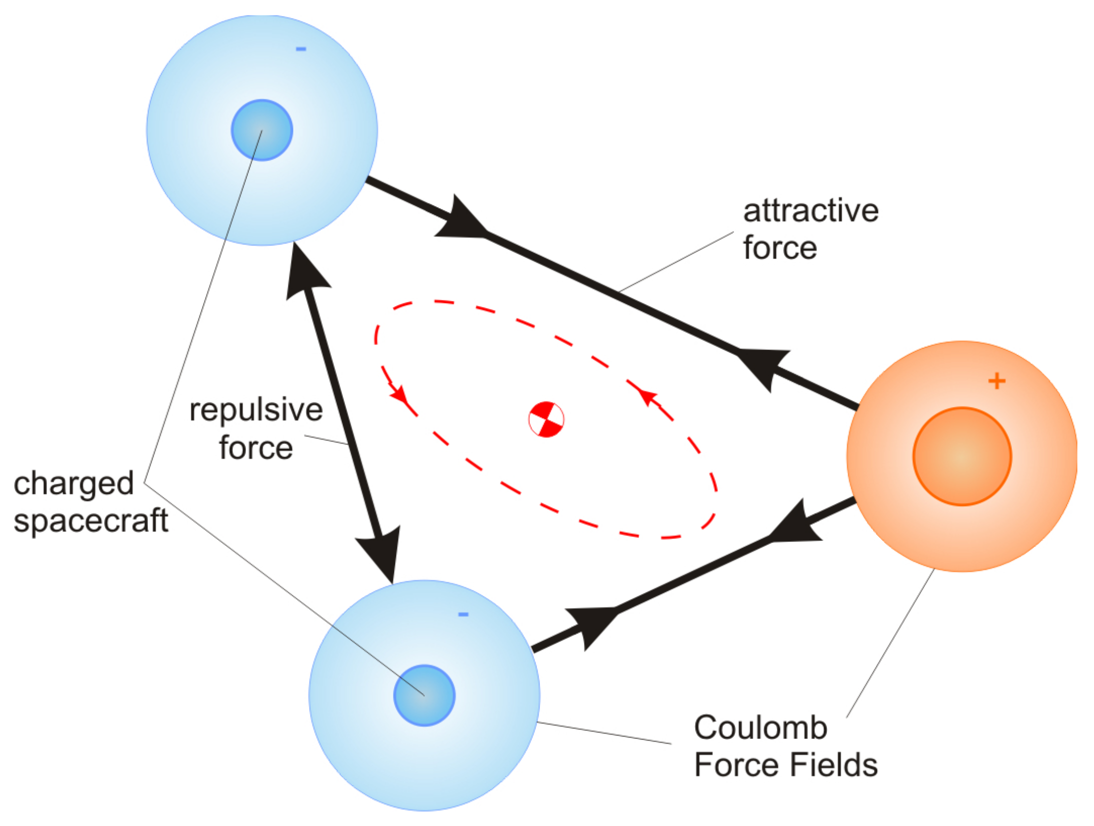
In [100], the generality of the problems of three bodies rotation under the action of gravitational and electrostatic forces is investigated for finding invariant forms. A schematic illustration of the structure discussed in [100] is shown in Figure 1. Hussein and Schaub [39] examined the general relative equilibria of such a system, and also discusses the stability of an open-loop system. It is assumed that the charged spacecraft moves in circular heliocentric orbits, far from the gravitational potential fields of planets or other celestial, bodies, therefore Hussein and Schaub [39] did not take into account the relative gravitational forces and focuses on the motion of freely moving bodies under the influence of electrostatic forces. In [39], general conditions are obtained, the solutions of which are relative equilibria for a rotating group of three spacecraft with Coulomb cables. Using the methods of linear control theory, stabilizing feedback is obtained in the form of PD and PID controllers for a nonlinear system, which guarantees its convergence to the neighborhood of the desired relative equilibrium. It is noted that for asymptotic stabilization of the desired relative equilibrium, independent of the value of the angular momentum h, it will be necessary to change the nominal equilibrium value of the charge in order to reflect the actual value of the angular momentum of the system. It is also indicated that the use of general methods of nonlinear stabilization can provide larger regions of stability than the methods based on linearization considered in [39].

The decentralized state estimation algorithms and their application to the spacecraft group are discussed in [101], where three main architectures are considered:

Centralized—only one point is involved, which performs primary calculations for a group of devices based on data collected at remote sites.

Decentralized—each apparatus in the group is involved, making an equal contribution to the assessment process. Each unit performs its own calculations based on the data obtained either as measurements or on the basis of the data transmitted from the entire group. In a decentralized architecture, there is no central entity to unify results.

Hierarchical—includes hybrids of the above two architectures. The large spacecraft group can be divided into smaller ones, each with its own architecture and grading system.

The simulation results given in [101] show that the decentralized reduced-order filter leads to simultaneous close to optimal estimates, as well as to the balance of communication and computational resources between the spacecraft. In addition, Ferguson and How [101] presented a hierarchical architecture for embedding decentralized assessment systems when scaling a problem for a large number of spacecraft in a group, as well as a necessary condition for a communication topology that guarantees the stability of the operation of simultaneously parallel computers and controllers.

The purpose of the research presented in [102] is an analysis of the dynamics of orientation and control of a connected satellite formation moving where the connected nodes are modeled as extended rigid bodies. Ref. [102] uses a three-in-a-row structure, and the general formula for the equations of motion of the system is obtained using the Lagrange method. The motions of the associated satellite system are analyzed in a three-dimensional coordinate system in outer space. The System Dependent Riccati Equation Regulator (SDRE) is used to eliminate orientation errors. The stability region for an SDRE-driven coupled satellite system is estimated numerically to show the global asymptotic robustness of the steering method. Centralized and decentralized approaches are applied to a dynamic system to compare targeting performance. It was found that the SDRE works well with both centralized and decentralized approaches to control the orientation of linked satellites in the formation of motion. The design of a formation flying orbit control system for LEO satellites based on the SDRE control approach may be also found in [103].

In [104], the problem of controlling the motion of an electromagnetic formation using the finite time method is investigated. The principle of electromagnetic formation flight (EMFF) uses magnetic fields electrically generated by all satellites, which then allows you to control the relative degrees of freedom. In EMFF, each satellite is equipped with three orthogonal magnetic coils and three orthogonal flywheels [105].

Zeng and Hu [104] presented an electromagnetic force model and analyzes the effect of the Earth’s magnetic field on EMFF satellites. Then, the equations of relative motion and the method for describing the general formation are established. The robust sliding mode controller is designed to track the trajectory in the presence of model uncertainties and external noise. The proposed controller, which combines the advantages of linear and terminal sliding mode control, can guarantee the convergence of tracking errors in a finite time, and not in an asymptotic sense. By constructing a specific Lyapunov function, the closed-loop system is proved to be globally stable and convergent. Numerical simulations of the maintenance and formation reconfiguration are then presented to show the efficiency of the designed controller.

Optimal reconfigurations of the Coulomb formation of two spacecraft are found in [106] using nonlinear optimal control methods. The aim of reconfigurations is to maneuver two spacecraft between two charged equilibrium configurations. Four optimality criteria are considered: minimum time, minimum separation acceleration, minimum use of fuel for an electric motor, and minimum power consumption. Reconfiguration between equilibria is first considered by changing the desired dilution distance. In the radial configuration of the relative equilibrium, only the Coulomb force is required to control the motion in the plane and to control the satellites from their initial to final radial positions. In this reconfiguration maneuver, the torque of the gravity gradient is used to stabilize motion in the plane. For equilibrium positions along the path and normal orbits, the reconfiguration maneuver requires hybrid control. Here, the Coulomb force is changed to control the separation distance, and the inertial micromotors are activated to control the lateral directions. Second, a reconfiguration involving hybrid steering is used to maneuver ships from any initial equilibrium position to a final one. The goal is to determine optimal maneuvers that maximize the use of the Coulomb propulsion unit while minimizing the use of the electric propulsion unit. The formulation of the two-point boundary value optimization problem is numerically solved using pseudospectral methods. The Pontryagin minimum principle checks the optimality of solutions without feedback.

In [107], a quaternion-based approach is considered for solving the time-limited problem of synchronizing and stabilizing satellites while moving in a formation. Sufficient conditions are given for the finite temporal convergence and stability of the distributed consensus problem. The nonlinear control law based on the finite time control method is designed in such a way that the exact position of the spacecraft will be consistent and will converge to the leader’s position, while the angular velocity will converge to zero in a finite time. A term in the form of an integral of a power function has been added to the Lyapunov function. In order to reduce the load on the network, a modified control law is proposed, where an estimate of the sliding mode with time constraints is introduced. This aims to ensure that only one satellite communicates with the leader. The modeling results are presented, showing the efficiency of the proposed method and its potential advantages.

Nair et al. [108] dealt with the development of a formation control strategy for a circular satellite constellation formation. In [108], the artificial potential field method is used to plan the trajectory, and the sliding mode control method is used to create a robust controller. The fuzzy inference engine is used to reduce the chattering phenomena inherent in conventional sliding mode systems. An algorithm for adaptive tuning of tuning a fuzzy parameter is derived on the basis of the Lyapunov stability theory. The proposed method based on a fuzzy system with a sliding mode is intended to compensate for the model uncertainties in practical applications. The simulation results for a group of five satellites forming a circular formation confirm the stability and robustness of the proposed scheme.

The purpose of [109] is to investigate the control of an electromagnetic tethered satellite system using Model Predictive Control (MPC). An electromagnetic tethered satellite system is powered by electromagnetic coils to generate control forces. The dynamic system model is described with high and low levels of accuracy, which are used to design the control system. Several horizons of the predictive model are used to bring the formation to the desired state. The presented control law not only satisfies the input and output constraints but also has the corresponding characteristics of optimality. The main advantage of using multiple horizons is multiple control based on predictive models, having a lower computational load compared to classical MPC. The results of numerical simulation and their comparison with sliding mode control are presented to demonstrate the effectiveness of the proposed control method and its advantages over both classical MPC control methods and sliding mode. The results obtained show a dramatic reduction in computational time and energy consumption compared to the classical MPC control methods and the sliding model, respectively.

4. Leader–Follower Formation Architecture

Fulfillment of the laws of linear control for the satellites formation in the presence of gravitational disturbances is considered by Sparks [110]. The use of a linear quadratic controller that minimizes the error between the actual and the required relative motion of the satellite is evaluated for the ability to maintain a specific geometry of the formation in the presence of such a gravitational disturbance as the uneven gravity of the Earth. The required formation geometry is based on solving linear equations of relative motion without disturbances. In particular, a group of satellites is selected whose projected motion onto the tangential plane of the Earth is a circle with a radius of one kilometer. It is shown that linear control laws support the formation within the error in the presence of gravitational disturbances. In addition, the simulation provides an estimate that takes into account the required fuel consumption to maneuver such a formation, thereby providing studies based on reducing costs while moving along the desired trajectories and according to the selected control strategies.

In [111], the formation control problem is considered in the following general setting. A complex system consisting of many subsystems (mobile agents) is described by the following equations

$$\begin{array}{c}\hfill {\dot{x}}_i=f_i(x_i,u_i,r_i),y_i=h_i\left(x_i\right),i=1,\cdots ,k\end{array}$$

(43)

where k is the number of subsystems; $x_i \in {\mathbb{R}}^{n_i}$ is the state vector of the i-th subsystem; $r_i$ express interrelations between subsystems and are defined as functions of $(x_j,u_j)$ for $i\ne j$; $u_i \in {\mathbb{R}}^{m_i}$ denotes the control input action of the i-th subsystem, $y_i=h_i\left(x_i\right) \in {\mathbb{R}}^p$ is the subsystem’s output. For example, for a formation of land vehicles, $h_i$ corresponds to the coordinates of each vehicle. It is considered that p is the same for all subsystems. Formation is defined in the coordinate system moving along with the desired trajectory $y_d\left(s\right) \in {\mathbb{R}}^p$, where s is a certain parameter, and the orthonormal vector $\mathcal{F}\left(s\right)=\left[{\mathbf{e}}_1\left(s\right),\cdots ,{\mathbf{e}}_p\left(s\right)\right] \in {\mathbb{R}}^p$, specifying a moving RMS, start which lies at the point $y_d\left(s\right)$. The formation F is thus specified by k by the points $P_1,\cdots ,P_k\in \mathcal{F}\left(s\right)$, $F=\{P_1,\cdots ,P_k\}$, where $P_i={\sum }_{j=1}^p{\alpha }_{ij}{\mathbf{e}}_j$, and in the general case it changes over time.

The key parameter is defined as the action reference s, on the basis of which the desired trajectory $y_d\left(s\right)$ is formed. To calculate the reference action, the reference projections are used, which transform the sensor data into a reference action s, on the basis of which the time is then calculated, which is used to coordinate lower-level feedbacks. The synthesis of the control law consists of several steps. On the first of them, given $y_d\left(s\right)$ and $\{P_1,\cdots ,P_k\}$, the desired trajectory $y_{di}\left(s\right)=y_d\left(s\right)+{\sum }_{j=1}^p{\alpha }_{ij}{\mathbf{e}}_j\left(s\right)$ for each agent (subsystem) in the formation is found. The speed of the formation along the trajectory $y_d\left(s\right)$ is specified by means of a strictly increasing function $s=v\left(t\right)$. The formation control law $u=u\left(x\right)$ must ensure the fulfillment of the control goal as $\underset{t\to \infty }{lim}\left(y_i\left(t\right)-y_{di}\left(v\left(t\right)\right)\right)=0$. With this control, there is an initial state $x_0={[x_{01},\cdots ,x_{0k}]}^{\mathrm{T}}$ such that the corresponding trajectory $x_{di}\left(s\right)$ coincides with the given one, that is, $h_i\left(x_{di}\left(s\right)\right)=y_{di}\left(t\right)$. In the second step, the control law $u_i=u_i(x,t)$ is synthesized separately for each subsystem using existing tracking methods ( signal tracking) or movement along a given trajectory ( path following). Different methods of controller synthesis can be used for different subsystems. To coordinate the subsystems, the third step uses the projection mapping. A reference projection is defined as a transformation $s=\gamma \left(x\right)$ such that $\gamma \left(x_d\left(s\right)\right)=s$, that is, if the state $x_d\left(s\right)$ is on the desired trajectory, then $\gamma$ must give the corresponding value of s also on the desired trajectory $x_d\left(s\right)$. For example, for any state $x_0$, vector $x_d\left(s_0\right)$ can be an orthogonal projection of $x_0$ onto $x_d\left(s_0\right)$. Orthographic design is not the only way to define $\gamma$, and changing it can fundamentally change the way of subsystems mutual coordination. The last stage of the controller design is the synthesis of a non-time-based feedback law that is used to control a multi-vehicle system. The control law is obtained by simple substitution and has the form

$$\begin{array}{c}\hfill u_i\left(x\right)=u_i\left(x,T\left(x\right)\right),T\left(x\right)=v^{-1}\left(\gamma \left(x\right)\right).\end{array}$$

(44)

A number of examples for selecting reference projections to ensure coordination of the formation are presented in [111]. In particular, the satellite clusters, forming a high-resolution synthetic aperture imaging formation are described. A flat formation consists of a group of satellites occupying the same orbital plane $OXY$ in the inertial terrestrial coordinate system $OXYZ$ and separated by the mean anomaly. The desired trajectory of movement of each satellite is considered to be a circular orbit of radius $r_0$ as

$$\begin{array}{c}\hfill x_d=r_{0}cos\left(\omega t\right),y_d=r_{0}sin\left(\omega t\right).\end{array}$$

(45)

As is known, $\omega ={\left({\displaystyle \frac{\mu }{r_0^3}}\right)}^{1/2}$, $\mu =3.986\times {10}^{14}$ m${}^3$/s${}^2$.

Following [112], the synthesis of the control law in [111] is performed by the feedback linearization method. For a near-circular orbit, the reference action s is defined as $s=\theta$, where $\theta$ is the angle between the satellite radius vector and X-axis on the $OXY$ plane. For the desired trajectory, $\theta =\omega t$. The relative position of satellites in the formation is determined through ${\gamma }_i$. For example, one can accept

$$\begin{array}{c}\hfill {\gamma }_1={\theta }_1,{\gamma }_2={\theta }_1-{\theta }_0,{\gamma }_3={\theta }_3,{\gamma }_4={\theta }_3-{\theta }_0,\end{array}$$

(46)

where ${\theta }_0$ is the desired angle between two satellites in the formation. According to (46), satellites $\#1$, $\#3$ are the leaders of the formation. Kang et al. [111] presented the theorems on the stability of the formation and the simulation results of the formation reconfiguration during movement.

Milam et al. [113] discussed the positioning and reorientation control of a formation of fully steerable low-thrust microsatellites. A general control methodology based on optimization is proposed for solving the problems of constructing a limited trajectory for positioning and reorientation. Taking advantage of the all-wheel drive microsatellites, onboard calculations can be performed on them. The software package Nonlinear Trajectory Generation (NTG) was used for typical space missions.

A systematic approach for studying the formations of multi-agent systems is presented in [114]. In particular, undirected formations for centralized formations and directed formations for decentralized formations, are considered. Paper [114] focuses on the feasibility problem: given the kinematics of multiple agents together with inter-agent constraints, one should find out if there are agent trajectories satisfying constraints. If the answer is yes, the task is to find a “smaller” control system that supports the movement of the formation along its trajectory, which, from the side of higher control levels, allows one to consider the formation as a whole. In [114], n heterogeneous agents with states $x_i\in M_i$, $i=1,\cdots ,n$ are considered. The agent’s kinematics are described by drift-free controlled distributions [115,116] on manifolds $M_i$ as

$$\begin{array}{cc}& {\Delta }_i:M_i\times U_i\to M_i,\hfill \\ & {\Delta }_i=\sum _j{X}_j{u}_j,\hfill \end{array}$$

(47)

where $U_i$ is the control space, the vector fields $X_i$ form the distribution basis. Controlled distributions are general enough to describe an underactuatio. The formation of a group of agents is determined by its graph, which completely describes the kinematics of individual agents and global inter-agency constraints. The graph of the formation $F=(V,E,C)$, consists of: a finite set V of vortices, the cardinality of which is number of agents, where each vertex $v_i:M_i\times U_i\to T{M}_i$ is a distribution ${\Delta }_i$ describing kinematics of each individual agent according to (47); binary relation $E\subset V\times V$, representing communication between agents; families of constraints C indexed by the set E, $C={\left\{c_e\right\}}_{e\in E}$. Two different types of formation graphs are considered: undirected formations, where $(V,E)$ is an undirected graph, and directed formations, where $(V,E)$ is a directed graph. In [114], conditions are obtained for determining formation feasibility for two types of formations, and also a management abstraction for a group is found, which allows one to describe a formation as a single object. When directional formation is not feasible it is possible to extract a feasible formation by eliminating the degrees of freedom that cannot be worked out by the follower agents.

In [117], nonlinear equations of orbital dynamics of relative motion are introduced for the problem of motion in a formation with separation into constant distances. This general equation of orbital dynamics allows for elliptical, non-coplanar maneuvers at large distances between spacecraft, as well as typical near-circular, coplanar maneuvers at short distances. In addition, changes in the equations of position and velocity have been introduced for a path in the plane of a formation with a large, constant separation angle between satellites. A nonlinear control method with the Riccati equation depending on the state is used to solve the problem of controlling the movement of the formation. This new control method for a non-linear system provides a clear design trade-off between control action and state error, similar to the classical linear quadratic control method. Numerical modeling shows the effectiveness of the new control method with the Riccati equation depending on the state with the developed equations of relative motion.

Palmer [118] presented a general analytical formulation of the problem for optimal trajectories of satellites flying in a formation, based on the circular version of Hill’s problem. Optimization is performed to minimize the displacement energy received from the motor. The optimization problem is the choice of the trajectory along which the satellite should move during the maneuver, while the required time and boundary conditions are fixed. Low thrust engines are suitable for maneuvering in formation. It is assumed that the engine is running throughout the entire maneuver, and the optimal program calculates the magnitude and direction of the thrust as a function of time. The possibility of using your own dynamics to obtain additional fuel economy by changing the boundary conditions is considered.

A method for constructing a satellite trajectory capable of creating a formation of a given configuration from identical spacecraft is given in [119]. The method uses a behavior-based approach to implement autonomous and distributed control of relative configuration using limited sensor information. For each satellite, the desired speed is defined as the sum of the various components of the general high-level behavior patterns. Further, the model of behavior is determined by an inverse dynamic calculation called the formation of equilibrium. Introduced several feedbacks for speed control. The results of the study show that in the developed method it is advisable to use control in a sliding mode.

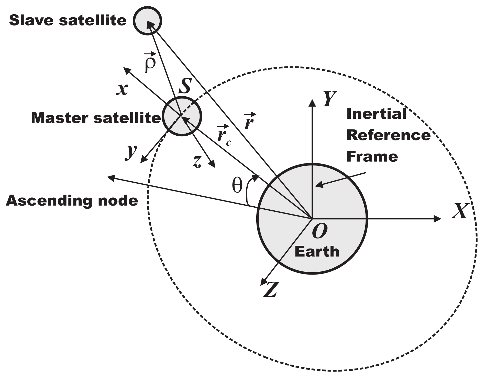
Kumar et al. [120] discussed achieving a given formation using thrust only in the direction along the trajectory. A system consisting of the leading satellite and the following satellites is considered, and linear control law is developed to obtain a formation of a given type. The orbital motion of the leader satellite is determined by the radial distance $r_c$ from the center of the Earth and the true anomaly $\theta$. The movement of the slave satellite is described with respect to the movement of the leader satellite using the relative r.m.s. S-xyz, anchored in the center of the leader satellite. The x-axis is directed along the local vertical, the z-axis is taken along the normal to the orbital plane, and the y-axis represents the third axis of this selected right RMS. The geometry of the orbital motion of the lead and slave satellites according to [120] is shown in the Figure 2. The orbital equations of motion for the lead satellite and the equations of motion of the slave satellite relative to the lead satellite are of the form [21,23]

$$\begin{array}{cc}& {\ddot{r}}_c-r_c{\dot{\theta }}^2+{\displaystyle \frac{\mu }{r_c^2}}=0,\hfill \end{array}$$

(48)

$$\begin{array}{cc}& r_c\ddot{-}\theta +2\dot{\theta }{\dot{r}}_c=0,\hfill \end{array}$$

(49)

$$\begin{array}{cc}& \ddot{x}-x{\dot{\theta }}^2-2\dot{y}\dot{\theta }-y\ddot{\theta }=-{\displaystyle \frac{\mu }{r^3}}(r_c+x)+{\displaystyle \frac{\mu }{r_c^2}}+f_{dx},\hfill \end{array}$$

(50)

$$\begin{array}{cc}& \ddot{y}-y{\dot{\theta }}^2+2\dot{x}\dot{\theta }+x\ddot{\theta }=-{\displaystyle \frac{\mu }{r^3}}y+f_y+f_{dy},\hfill \end{array}$$

(51)

$$\begin{array}{cc}& \ddot{z}=-{\displaystyle \frac{\mu }{r^3}}z+f_{dz},\hfill \end{array}$$

(52)

where $r=({(r_c+x)}^2+y^2+z^2{)}^{1/2}$; $f_y$ is the acceleration of the control force in the longitudinal direction; $f_{dj}$, $j\in \{x,y,z\}$ are the accelerations of the disturbing force along the directions x, y and z, respectively. To synthesize the control law, the following linearized model of the (50)–(52) system is used, obtained under the assumption that the leading satellite is moving in a circular orbit

$$\begin{array}{cc}& \ddot{x}-2\dot{\theta }\dot{y}-3{\dot{\theta }}^{2}x=0,\hfill \end{array}$$

(53)

$$\begin{array}{cc}& \ddot{y}+2\dot{x}\dot{\theta }=f_y,\hfill \end{array}$$

(54)

$$\begin{array}{cc}& \ddot{z}+{\dot{\theta }}^{2}z=0,\hfill \end{array}$$

(55)

where $\dot{\theta }=const$ is taken.

In [120] the following linear proportional-differential (PD) control law is proposed

$$\begin{array}{cc}& f_y=k_{p1}(x-x_d)+k_{d1}(\dot{x}-{\dot{x}}_d)+k_{p2}(y-y_d)+k_{d2}(\dot{y}-{\dot{y}}_d),\hfill \end{array}$$

(56)

where $x_d$, $y_d$ are the desired (specified) values of the coordinates x, y, $k_{p1}$, $k_{d1}$, $k_{p2}$, $k_{d2}$ are the regulator coefficients.

The performance of the proposed regulator was investigated by the Routh–Hurwitz criterion and tested using the simulation of nonlinear equations of motion of the system taking into account several factors, including changes in the initial conditions, the size of the formation, the presence of disturbing forces and eccentricity of the orbit of the lead satellite. It was found that a regulator using only thrust along the trajectory can provide a bounded relative position error, without damping, with a maximum control acceleration (in m/s${}^2$) of $0.0718{\dot{\theta }}^2$ times the error along the trajectory and, therefore, has a limited ability to neutralize disturbances. However, by modeling, it was found that the proposed controller successfully provided limited relative position errors below $\pm 10$ m.

Sengupta et al. [121] presented expressions describing the average relative motion of two satellites in adjacent orbits around a planet flattened at the poles. The theory assumes small relative distances between satellites, which is equally true for all elliptical orbits, as well as for the special case of a circular orbit due to the use of nonsingular orbital elements. An analytical filter has been introduced, which compensates for short-period changes in the relative state without using built-in digital filters, which are usually used to filter noise in the design of control systems. The application of this filter to maintain the formation on a given relative trajectory is considered.

In [122], orbital elements are defined as a set of parameters that characterize the relative motion of a satellite formation based on the principle of geostationary spacecraft control. From these parameters, the orbital motion and maneuvering equations are derived. In addition, in [122], acceleration control laws are proposed, including out-of-plane and in-plane control. To demonstrate them as orbital maneuvers, the following are considered: the creation of a formation of two satellites, its reconfiguration, maneuvering at long distances, and the preservation of the formation. The results of modeling the dynamics of the movement of the formation under the influence of the gravitational field and eccentricity when applying the proposed law of control with feedback are presented, which show the effectiveness of the proposed method and the possibility of correct control of the slave satellite from the lead satellite.

In [123], simple and general analytical solutions are considered for the optimal reconfiguration of a satellite constellation controlled by various linear dynamic equations. The calculus of variations is used for the analytical search for optimal trajectories and control. The proposed method makes it possible to predict in advance the exact form of optimal solutions without the need to solve the problem. It is shown that the optimal thrust vector as a function of the fundamental matrix of the given equations of state. The analytical solutions presented in this paper can be applied to most problems of satellite reconfiguration governed by linear dynamic equations. Numerical modeling confirms the brevity and accuracy of the solutions obtained.

During the LISA missions [9], it may be necessary to reconfigure the formation to maintain or improve its functionality [10]. This reconfiguration can be described by relative dynamics, as presented, for example, in [23,124]. Using relative dynamics in projection onto a circular orbit, the authors of [17] found analytical solutions for optimal two-pulse trajectories of reconfiguration of a formation of two spacecraft in orbit. The desired formation is characterized by nonsingular different orbital elements. To achieve the desired orbital-element differences, [17] proposes an analytical two-pulse solution found using the Gaussian variational equations. The solutions obtained can be easily implemented using onboard computing devices. In order to maximize mission life during reconfiguration, many papers consider the problem of optimization in terms of fuel consumption. The works by Kurzhansky and his colleagues significantly developed a solution to the problem of control synthesis for impulsive systems, based on generalizations of the Hamilton–Jacobi–Bellman variational inequalities, which made it possible, within the framework of a single formalization, to study control problems for hybrid systems containing jump-like rearrangements of states [125,126].

Optimization methods based on the calculus of variations, including the theory of basis vectors, encounter difficulties in finding the global optimal solution, since these methods can only search in a convex neighborhood around the initial approximation. Therefore, the global optimality of the solution is not guaranteed, especially with substantially non-convex objective functions. To mitigate these difficulties, several methods have been proposed, one of which is the “hybrid optimization”—a combination of the calculus of variations and global extremum search [127,128]. Paper [10] is apparently the first attempt to use hybrid optimization with a genetic algorithm to find reconfiguration trajectories, although the genetic algorithm has often been used for other trajectory optimization problems. In [10], the relative motion in the LVLH reference frame is described using the HCW equations of motion.

The satellite constellation consists of a head satellite and surrounding slave satellites. The orbit of the lead satellite is considered a reference orbit, and the relative orbits of the follower are considered to be PCO. PCO predicted distances between the master and slave satellites [129] are constant. The HCW equation describes the relative motion between the master and slave satellites in the local reference frame LVLH with the origin on the master satellite. In this system, the $OX$ axis is defined in the radial direction of the main orbit, and the $OY$ axis is defined as the longitudinal direction of the main orbit. The $OZ$ axis is defined to complete the right coordinate system. The relative position vector $\mathbf{r}$ and the relative velocity vector $\mathbf{v}$ of the slave satellite are defined in the LVLH reference system. State vector $\mathbf{x}$ of relative dynamics is defined as $\mathbf{x}=\begin{array}{cc}[{\mathbf{r}}^{\mathrm{T}}\hfill & {\mathbf{v}}^{\mathrm{T}}\hfill \end{array}{]}^{\mathrm{T}}$, where $\mathbf{r}={\left[\begin{array}{ccc}x\hfill & y\hfill & z\hfill \end{array}\right]}^{\mathrm{T}}$, $\mathbf{v}=\begin{array}{ccc}[\dot{x}\hfill & \dot{y}\hfill & \dot{z}\hfill \end{array}{]}^{\mathrm{T}}$. Then, [10] displays the linearized equation of relative motion for two bodies. The distances between the master and slave satellites are ignored during linearization since they are significantly less than the distance between the main satellite and the center of gravity (Earth, when moving in the LEO). Thus, the linear equations of state are obtained

$$\begin{array}{cc}& \dot{\mathbf{x}}\left(t\right)=\left[\begin{array}{cc}{\mathbf{O}}_3& {\mathbf{I}}_3\\ \mathbf{A}& \mathbf{B}\end{array}\right]\mathbf{x}\left(t\right),\mathbf{A}=n^2\left[\begin{array}{ccc}3& 0& 0\\ 0& 0& 0\\ 0& 0& -1\end{array}\right],\mathbf{B}=n\left[\begin{array}{ccc}0& 2& 0\\ -2& 0& 0\\ 0& 0& 0\end{array}\right],\hfill \end{array}$$

(57)

where ${\mathbf{O}}_3$, ${\mathbf{I}}_3$ are the zero and unit matrices of order 3, $n=\sqrt{GM/a^3}$ is the average speed of the lead spacecraft, G is the gravitational constant, M is the mass of the central body (for the Earth, $GM=398,603·{10}^9{\mathrm{m}}^3·{\mathrm{c}}^{-2}$), a is the semi-major axis of the orbit of the lead satellite. The homogeneous Equations (57) are then analytically integrated using the Cauchy formula $\mathbf{x}\left(t\right)=\Phi \mathbf{x}\left(0\right)$, where $\Phi =exp\left(\left[\begin{array}{cc}{\mathbf{O}}_3& {\mathbf{I}}_3\\ \mathbf{A}& \mathbf{B}\end{array}\right]t\right)$ is the fundamental matrix of the system (57), $t⩾0$ stnads for the current time, $\mathbf{x}\left(0\right)$ denotes the initial state vector. (There are some inaccuracies in this expression for matrix $\Phi$ in [10].)

Kim et al. [10] explored the three types of reconfiguration maneuvers described in [73] namely resizing, reassigning, and reorienting. Resizing is the change in distance between spacecraft in the formation. In [10], a hybrid optimization strategy with a genetic algorithm and basis vector theory is used for fuel-optimal reconfiguration of a satellite group. In hybrid optimization, the genetic algorithm performs a global search to create two-impulse trajectories at each transition time, and vector analysis of basis vectors serves for local optimization with two-impulse trajectories as initial approximations. The final optimal trajectory has multiple pulses and also lower fuel consumption than two-pulse trajectories. The mission planner must investigate the trade-off between fuel saved by multiple impulses and the increased mission complexity due to additional impulses. In many missions, the trajectory obtained by the genetic algorithm will have an advantage for the transition due to its simplicity and almost optimal fuel consumption.

The Udwadia–Calaba method is used in [130], where under the assumption of unlimited and time-varying throttle starts throughout the entire maneuver, precisely and explicitly without any restrictions on the distance between satellites, the formation retention problem is solved. Cho and Yu [130] discussed a system of two satellites orbiting a central body (around the Earth). One of them is called the “master”, and the other is the “deputy” satellite, which must maintain a given location relative to the head. The equation of motion of two bodies for an inertial frame of reference is used, which is supplemented by the requirement to hold the station as constraints for obtaining an equation of motion that fully takes into account all nonlinearities. From this, the governing force is derived as an explicit function of state and time required to maintain the formation. The results obtained are also applicable to the case when the distance between the satellites is so great that the linearized relative equations of motion are not applicable. The dynamics described in the inertial frame of reference is then transformed for convenience into a local moving frame of reference through the transformation matrix. As a practical limitation, in [130] a relative configuration that is circular when projected onto the local horizontal plane is chosen. It is commonly referred to as the PCO [129,131]. Unrestricted motion is relative motion without a control force acting on the satellite system. The master and slave satellites move only under the influence of gravity, and therefore “unlimited” and uncontrolled motions have the same meaning. In the case of movement with restrictions, control forces must be applied to the system. Therefore, “limited” and “controlled” movements also have the same meaning. When a satellite with a point mass orbits the Earth, its acceleration $\mathbf{a}$ is written in the Earth’s inertial coordinate system as follows [132]:

$$\begin{array}{c}\hfill \mathbf{a}=-{\displaystyle \frac{GM}{{\left(X^2+Y^2+Z^2\right)}^{3/2}}}\left[\begin{array}{c}X\\ Y\\ Z\end{array}\right]\end{array}$$

(58)

where G is the universal gravitational constant, M is the mass of the central body (the mass of the Earth). The Equation (58) is written in the inertial terrestrial coordinate system originating from the center of the Earth, the X axis points to the vernal equinox, the Z axis passes through the North Pole, and the Y axis completes the right n.v. (see Figure 3).

Assuming that the master satellite is in a circular orbit with a fixed inclination without any disturbance, the goal is to maintain a constant distance between it and the follower, for example, when projecting onto the local horizontal plane. In addition, to prevent discrepancy in X coordinate, a constraint is also applied between the X and Z coordinates. Hill’s LVLH coordinate system [21,23] is used to describe these limitations. The origin of this system is located on the leading satellite, X-axis lies in the radial direction, Y-axis is in the path direction, and Z-axis lies along the orbital angular momentum vector, thus completing the right-handed coordinate system see Figure 3. In LVLH coordinate system, the constraint equations can be written as

$$\begin{array}{cc}& y^2+z^2={\rho }^2,\hfill \end{array}$$

(59)

$$\begin{array}{cc}& 2x-z=0,\hfill \end{array}$$

(60)

where $\rho$ is the constant distance between satellites. Since the Equations (59) and (60) describe holonomic constraints, they are twice differentiated in time, which gives

$$\begin{array}{cc}& y\ddot{y}+z\ddot{z}=-{\dot{y}}^2-{\dot{z}}^2,\hfill \end{array}$$

(61)

$$\begin{array}{cc}& 2\ddot{x}-\ddot{z}=0.\hfill \end{array}$$

(62)

Further, in [130], transformations of the rotation of variables from the Earth’s r.s. to the Hill coordinate system are performed

$$\begin{array}{c}\hfill \left[\begin{array}{c}x+r_0\\ y\\ z\end{array}\right]=\mathbf{R}\left[\begin{array}{c}X\\ Y\\ Z\end{array}\right]\end{array}$$

(63)

with the rotation matrix $\mathbf{R}$, depending on the longitude of the ascending node of the lead satellite $\Omega$, the angle between the equatorial plane and the orbital plane of the lead satellite i, latitude of the lead satellite $\omega ={\omega }_0+n(t-t_0)$, $n=\sqrt{{\displaystyle \frac{GM}{r_0^3}}}$, and the radius $r_0$ of the circular orbit of the lead satellite.

This circular is based on linearized equation solutions, and therefore non-linear behavior of relative motion will violate this configuration. To avoid this, additional control force is used. The approach of [130] provides a general methodology that can be easily applied to any type of relative configuration. To solve the problem in [130], further transformations of constraints are performed (61) and (62) to the form (36) and then use (42). For this purpose, equations (59) and (60) are first reduced to the form

$$\begin{array}{cc}& \left[\begin{array}{cc}y& z\end{array}\right]\left[\begin{array}{c}\ddot{y}\\ \ddot{z}\end{array}\right]=-\left[\begin{array}{cc}\dot{y}& \dot{z}\end{array}\right]\left[\begin{array}{c}\dot{y}\\ \dot{z}\end{array}\right],\hfill \end{array}$$

(64)

$$\begin{array}{cc}& \left[\begin{array}{cc}2& -1\end{array}\right]\left[\begin{array}{c}\ddot{x}\\ \ddot{z}\end{array}\right]=0.\hfill \end{array}$$

(65)

Finally, the system equations are reduced to the form [81]:

$$\begin{array}{cc}& \ddot{\mathbf{x}}+\mathbf{a}+{\mathbf{A}}^{†}(\mathbf{b}-\mathbf{A}\mathbf{a}),\hfill \end{array}$$

(66)

$$\begin{array}{cc}& \mathbf{M}\ddot{\mathbf{x}}=\mathbf{F}+\mathbf{M}{\mathbf{A}}^{†}(\mathbf{b}-\mathbf{A}\mathbf{a}),\hfill \end{array}$$

(67)

whence the expression for the control force ${\mathbf{F}}^c$ is derived:

$$\begin{array}{c}\hfill {\mathbf{F}}^c=\mathbf{M}{\mathbf{A}}^{†}(\mathbf{b}-\mathbf{A}\mathbf{a}).\end{array}$$

(68)

The presentation is illustrated by numerical examples. It is worth mentioning that in [130] there are no explicit restrictions on either the control action or the fuel consumption.

Simple and accurate formation control schemes are presented by Cho and Udwadia [133], where a method of analytic dynamics by Udwadia [76], Udwadia and Kalaba [77], Udwadia [78,79] is employed. In [133], the explicit control inputs for accurately maintaining a given formation configuration, using continuous thrust systems, are found. A much simpler and more explicit expression is obtained to accurately satisfy the formation conservation constraints for Keplerian reference orbits. Cho and Udwadia [133] also includes explicit control results when the follower is put into orbit with incorrect initial conditions, as is usually the case in practice. Extensive computational simulations demonstrate that the approach of [133] is easy to implement and numerically precise.

The problems of attitude synchronization and tracking in the spacecraft formation in the presence of model uncertainties and external interference are considered by Wu et al. [134]. A decentralized control law for the adaptive slip mode using the topology of undirected communication between spacecraft is proposed, which is analyzed on the basis of the theory of algebraic graphs. A sliding manifold is obtained for several spacecraft, on which each spacecraft approaches the desired time-varying orientation and angular velocity, while maintaining orientation synchronization with other spacecraft in the formation. Next, a control law is developed to ensure convergence to a sliding manifold. The stability of the resulting closed-loop system is proved by applying the Barbalat lemma. The simulation results demonstrate the effectiveness of the proposed synchronization and tracking methodology for orientation problems.

The problem of designing a distributed controller for a continuous time system consisting of a number of identical dynamically coupled subsystems is discussed in [135]. The main mathematical conclusion is based on the Kronecker product and a special similarity transformation built from a matrix of interconnection patterns that breaks the system into modal subsystems. This, along with the result of formulating the extended linear matrix inequality (LMI) for continuous-time systems, allows one to obtain explicit expressions for calculating the parameters of distributed controllers for both state feedback and dynamic output feedback. The main contribution of [135] is the solution of the distributed control problem for systems with continuous time under the conditions of $H_{\infty }/\alpha$-stability and $H_2/\alpha$-stability characteristics by solving the set of LMIs with non-common Lyapunov variables. The efficiency of this method is demonstrated by the example of a satellite formation.

Autonomous navigation of micro-UAVs is usually based on the integration of inexpensive Global Navigation Satellite System (GNSS) receivers and inertial and magnetic sensors based on microelectromechanical systems (MEMS) for motion stabilization and control. The resulting navigation performance in terms of position and orientation accuracy may be insufficient for other mission tasks, such as those related to precise sensor pointing. In this context, [136] introduces a collaborative UAV navigation algorithm that allows the main vehicle equipped with inertial and magnetic sensors, a global positioning system (GPS) receiver, and a vision system to improve its navigation performance (in real time or in real-time). The focus is on the outdoor environment, and the key concept is to use differential GPS (DGPS) among vehicles and vision-based tracking (DGPS/Vision) to create a virtual auxiliary navigation sensor, which information is then integrated into a sensor fusion algorithm based on an extended Kalman filter (EKF). The developed concept and processing architecture are described with an emphasis on the DGPS/Vision orientation determination algorithm. Efficiency assessment is carried out on the basis of numerical modeling and flight tests. In the latter of these, the navigation estimates obtained from the DGPS/Vision approach are compared with the estimates provided by the onboard autopilot system of the tuned quad. The analysis shows the potential of the developed approach, mainly due to the ability to use magnetic and inertial-independent accurate orientation information.

The distributed robust control method is developed relies, on a spaceborne distributed telescope, is presented in [137], where a combination of robust $H_{\infty }$ control and distributed control using the consensus approach is proposed, focused on the application to satellite formation motion.

The method of simultaneous control of the relative motion and orientation of the solar radiation pressure was proposed in [138]. The aim of the control is to stabilize a given closed relative orbit. The basic idea is to use special materials for solar sails that can change their optical properties. A solar sail consists of several rectangular cells. Each of them can change its optical properties. The required steering force is generated by varying the average reflectivity of the solar sail, and the steering torque is achieved using the appropriate black and white mesh pattern.

Mashtakov et al. [139] discussed the use of sunlight pressure to control a satellite formation. The control is based on the rotation of the sail normal, which provides for a change in the optical properties of its surface.

Monakhova et al. [140] dealt with the problem of satellite formation immediately after launch. When detached from the launcher, there is a certain error in the magnitude of the speed jump, which leads to slightly different periods of rotation of the satellites. As a result, relative paths become open. Differential control using a resistance force is considered. The satellite orientation is controlled by a magnetic actuator.

The problem of creating a robust formation controller for a group of satellites whose dynamics are associated with nonlinearities and uncertainties is considered by Liu et al. [141]. For a constellation of satellites, a formation adjuster is proposed that includes a position adjuster for the formation of the desired precise formation and a position adjuster for aligning the positions of the satellites. It is shown that errors in trajectory tracking and orientation of the entire closed-loop control system can converge to a given neighborhood of the origin in a finite time. Simulation results are presented to demonstrate the benefits of the proposed formation control scheme.

In [142], trajectory analysis, mission design, and the control law for several microsatellites for joint traversal of the spacecraft are considered. The problem of the cooperative movement of a group of satellites along an elliptical trajectory, i.e. cooperative circumnavigation, (CCN) is first defined to bring the group of microsatellites to a predetermined plane ellipse relative to the host spacecraft while maintaining the geometric configuration of the formation. Then, a CCN control law is proposed, in which artificial potential functions and the Laplace affine matrix are applied to fulfill the requirements of the CCN mission. Simulation results are presented to show the feasibility of this approach.

In [143], a joint navigation approach for unmanned aerial vehicles (UAVs) is presented, which makes it possible to reliably and accurately determine the orientation of the main aircraft flying in formation with other UAVs (alternates, slaves). The proposed method is based on a closely related extended Kalman filter using the spatial diversity of measurements from global navigation satellite systems (GNSS) and vision systems integrated with data from inertial and magnetic sensors. The main focus is on the external environment, and the innovative idea is to extend the attitude estimation approaches based on multiple GNSS antennas to a multipurpose system where differential GNSS and UAV visual tracking of UAVs are used to create a virtual auxiliary navigation sensor. The processing concept and architecture are described with an emphasis on an ECP measurement update phase that is applicable to any number of collaborating proxies and to different GNSS processing architectures. The effectiveness of the proposed method is evaluated by experimental tests using two multi-rotors and two fixed ground antennas, one of which is used as a ground reference point for the analysis of pointing accuracy. The results show the feasibility of the developed approach in terms of accuracy and providing drift-free estimates in real-time or in post-processing scenarios.

A group of four satellites forming a tetrahedron is discussed in [144]. The task is to maintain relative orbits so that the tetrahedron retains its shape and size over time according to the introduced criterion. The problem of constructing relative reference orbits of satellites is solved, which, within the framework of the linear HCW model, ensure the preservation of the tetrahedron parameters in the absence of control. In the framework of the Schweigart–Sedwick linear model [91,92], which takes into account the influence of the second harmonic of the geopotential, as well as in the framework of a nonlinear motion model with the second harmonic, algorithms are proposed for constructing uniaxial motion control of satellites oriented along the Earth’s magnetic field, which ensure the maintenance of relative orbits.

In [145], the task of controlling a group of four satellites in a low near-circular Earth orbit is considered. The satellites form a tetrahedron of a certain shape and size. The initial data were selected in such a way that the change in the shape and size of this tetrahedron during the movement of satellites in orbit was minimal. The choice of the initial data was carried out analytically and then numerically refined. Michael Ross et al. [146] presented an approach to solving a class of problems arising in the development of satellite swarms. The key issue addressed in this article is “simultaneous” fusion and orbit control to achieve swarm configuration. Although any design criterion can be used, a fuel consumption approach is used, since the fuel cost (loss) function is extremely high for a spacecraft (SC). It is shown how certain elements of the theory of optimal periodic control provide a very natural formulation of this problem. Using versatile dynamic optimization software it is shown how one can easily design satellite formations without using any analytical results. If a natural zero fuel solution does not exist, a byproduct of the proposed approach automatically determines the minimum amount of fuel and the associated controls required to maintain the formation.

5. Conclusions

This paper provides an overview of the results on the control of a formation flight of spacecraft, expanding and supplementing the review [1], related to 2004, with modern publications. Three types of formation architectures are considered: MIMO, in which the formation is treated as a single entity with multiple inputs and multiple outputs; LF, in which individual spacecraft controllers have linked hierarchically, and a virtual structure in which each spacecraft in formation is considered as a rigid body, embedded in a common virtual structure. The MIMO architecture differs from other ones in its optimality and stability. However, the use of all system states leads to the need to introduce high requirements on the information exchange, so such algorithms are usually unstable to local failures. The leader–follower architecture uses information about leaders only, which simplifies formation navigation. The problem of reliability is solved by increasing the number of leaders. However, this approach is inferior in optimality, and for ensuring high system stability, information requirements can reach those of the MIMO case. The cyclic architecture is a middle ground between LF and MIMO architectures. The information requirements are as high as those of MIMO case, and connections between some devices are allowed. However, round-robin algorithms can be completely decentralized. There is no coordinating agent and no instability due to single failures. In the process of research in this area, a number of directions have appeared in which, in particular, an increase in the stability and reliability of systems, reducing requirements for information restrictions, and increasing the spacecraft autonomy in formations. In the paper, examples of modern group spacecraft missions are also outlined.

References

- Scharf, D.; Hadaegh, F.; Ploen, S. A survey of spacecraft formation flying guidance and control. Part 1: Guidance. In Proceedings of the 2003 American Control Conference (ACC 2003), Denver, CO, USA, 4–6 June 2003; Volume 2, pp. 1733–1739. [Google Scholar] [CrossRef]
- Alfriend, K.T.; Vadali, S.R.; Gurfil, P.; How, J.P.; Breger, L.S. Spacecraft Formation Flying: Dynamics, Control and Navigation. In Spacecraft Formation Flying; Alfriend, K.T., Vadali, S.R., Gurfil, P., How, J.P., Breger, L.S., Eds.; Butterworth-Heinemann: Oxford, UK, 2010; p. iv. [Google Scholar] [CrossRef]
- D’Errico, M. Relative Trajectory Design. In Distributed Space Missions for Earth System Monitoring; D’Errico, M., Ed.; Springer: New York, NY, USA, 2013. [Google Scholar] [CrossRef]
- Schilling, K.; Loureiro, G.; Zhang, Y.; Nchter, A.; Scharnagl, J.; Motroniuk, I.; Aumann, A. TIM: An Int. nano-satellite formation for photogrammetric earth observation. In Proceedings of the Int. Astronautical Congress, IAC, Washington, DC, USA, 21–25 October 2019; Volume 2019. [Google Scholar]
- Schilling, K.; Schechner, Y.; Koren, I. CloudCT—A formation of cooperating nano-satellites for cloud characterisation by computed tomography. In Proceedings of the Int.Astronautical Congress, IAC, Washington, DC, USA, 21–25 October 2019; Volume 2019. [Google Scholar]
- Freimann, A.; Petermann, T.; Schilling, K. Interference-Free Contact Plan Design for Wireless Communication in Space-Terrestrial Networks. In Proceedings of the 2019 IEEE International Conference on Space Mission Challenges for Information Technology (SMC-IT), Pasadena, CA, USA, 30 July–1 August 2019; pp. 55–61. [Google Scholar] [CrossRef]
- Busch, S.; Bangert, P.; Dombrovski, S.; Schilling, K. UWE-3, in-orbit performance and lessons learned of a modular and flexible satellite bus for future pico-satellite formations. Acta Astronaut. 2015, 117, 73–89. [Google Scholar] [CrossRef]
- Folta, D.; Bordi, F.; Scolese, C. Considerations on formation flying separations for earth observing satellite missions. Adv. Astronaut. Sci. 1992, 79, 803–822. [Google Scholar]
- Bik, J.; Visser, P.; Jennrich, O. LISA satellite formation control. Adv. Space Res. 2007, 40, 25–34. [Google Scholar] [CrossRef]
- Kim, D.Y.; Woo, B.; Park, S.Y.; Choi, K.H. Hybrid optimization for multiple-impulse reconfiguration trajectories of satellite formation flying. Adv. Space Res. 2009, 44, 1257–1269. [Google Scholar] [CrossRef]
- Wu, S.F.; Fertin, D. Spacecraft drag-free attitude control system design with Quantitative Feedback Theory. Acta Astronaut. 2008, 62, 668–682. [Google Scholar] [CrossRef]
- Schilling, K. Small Satellite Formations: Challenges in Navigation and its Application Potential. In Proceedings of the 28th Saint Petersburg International Conference on Integrated Navigation Systems (ICINS 2021), Saint Petersburg, Russia, 31 May–2 June 2021. [Google Scholar]
- Kramer, A.; Schilling, K. First demonstration of collision avoidance and orbit control for pico-satellites—UWE-4. Acta Astronaut. 2021, 185, 244–256. [Google Scholar] [CrossRef]
- Mathavaraj, S.; Padhi, R. Satellite Formation Flying-High Precision Guidance Using Optimal and Adaptive Control Techniques; Springer: Singapore, 2021. [Google Scholar]
- Alfriend, K.T.; Vadali, S.R.; Gurfil, P.; How, J.P.; Breger, L. Spacecraft Formation Flying: Dynamics, Control and Navigation; Elsevier Ltd.: Oxford, UK, 2010. [Google Scholar]
- Schaub, H.; Vadali, S.; Junkins, J.; Alfriend, K. Spacecraft formation flying control using mean orbit elements. J. Astronaut. Sci. 2001, 48, 69–87. [Google Scholar] [CrossRef]
- Vaddi, S.; Alfriend, K.; Vadali, S.; Sengupta, P. Formation establishment and reconfiguration using impulsive control. J. Guid. Control Dyn. 2005, 28, 262–268. [Google Scholar] [CrossRef]
- Vassar, R.; Sherwoodt, R. Formation keeping for a pair of satellites in a circular orbit. J. Guid. Control Dyn. 1985, 8, 235–242. [Google Scholar] [CrossRef]
- Ulybyshev, Y. Long-term formation keeping of satellite constellation using linear-quadratic controller. J. Guid. Control Dyn. 1998, 21, 109–115. [Google Scholar] [CrossRef]
- Inalhan, G.; Tillerson, M.; How, J.P. Relative Dynamics and Control of Spacecraft Formations in Eccentric Orbits. J. Guid. Control Dyn. 2002, 25, 48–59. [Google Scholar] [CrossRef]
- Hill, G.W. Researches in the Lunar Theory. Am. J. Math. 1878, 1, 5–26. [Google Scholar] [CrossRef]
- Sedwick, R.; Miller, D.; Kong, E. Mitigation of Differential Perturbations. J. Astronaut. Sci. 1999, 47, 309–331. [Google Scholar] [CrossRef]
- Clohessy, W.; Wiltshire, R. Terminal guidance system for satellite rendezvous. J. Aerosp. Sci. 1960, 27, 653–658. [Google Scholar] [CrossRef]
- Lawden, D.F. Optimal Trajectories for Space Navigation; Butterworths: London, UK, 1963. [Google Scholar]
- Carter, T.E.; Humi, M. Fuel-Optimal Rendezvous near a Point in General Keplerian Orbit. J. Guid. Control Dyn. 1987, 10, 567–573. [Google Scholar] [CrossRef]
- Carter, T.E. New Form for the Optimal Rendezvous Equations near a Keplerian Orbit. J. Guid. Control Dyn. 1990, 13, 183–186. [Google Scholar] [CrossRef]
- Tillerson, M.; How, J. Formation flying control in eccentric orbits. In Proceedings of the AIAA Guidance, Navigation, and Control Conference and Exhibit, Montreal, QC, Canada, 6–9 August 2001. [Google Scholar]
- Schaub, H.; Alfriend, K.T. J2 Invariant Reference Orbits for Spacecraft Formations. In Proceedings of the Flight Mechanics Symposium, Goddard Space Flight Center, Greenbelt, MD, USA, 18–20 May 1999. [Google Scholar]
- Brouwer, D. Solution of the Problem of Artificial Satellite Theory Without Drag. Astronaut. J. 1959, 64, 378–397. [Google Scholar] [CrossRef]
- Battin, R. An Introduction to the Mathematics and Methods of Astrodynamcis; AIAA Education Series: Reston, Virginia, 1987. [Google Scholar]
- Schaub, H.; Alfriend, K. Hybrid Cartesian and orbit element feedback law for formation flying spacecraft. J. Guid. Control Dyn. 2002, 25, 387–393. [Google Scholar] [CrossRef]
- Williams, T.; Wang, Z.S. Uses of solar radiation pressure for satellite formation flight. Int. J. Robust Nonlinear Control 2002, 12, 163–183. [Google Scholar] [CrossRef]
- Hussein, I.; Scheeres, D.; Hyland, D. Control of a Satellite Formation For Imaging Applications. In Proceedings of the American Control Conference (ACC’2003), Denver, CO, USA, 4–6 June 2003; Volume 1, pp. 308–313. [Google Scholar]
- Gill, E.; Runge, H. Tight formation flying for an along-track SAR interferometer. Acta Astronaut. 2004, 55, 473–485. [Google Scholar] [CrossRef]
- Bamler, R.; Hartl, P. Synthetic aperture radar interferometry. Inverse Probl. 1998, 14, R1–R54. [Google Scholar] [CrossRef]
- Romeiser, R.; Breit, H.; Eineder, M.; Runge, H.; Flament, P.; de Jong, K.; Vogelzang, J. Current measurements by SAR along-track interferometry from a Space Shuttle. IEEE Trans. Geosci. Remote Sens. 2005, 43, 2315–2324. [Google Scholar] [CrossRef]
- Romeiser, R.; Johannessen, J.; Chapron, B.; Collard, F.; Kudryavtsev, V.; Runge, H.; Suchandt, S. Direct Surface Current Field Imaging from Space by Along-Track InSAR and Conventional SAR. In Oceanography from Space; Barale, V., Gower, J., Alberotanza, L., Eds.; Springer: Dordrecht, The Netherlands, 2010. [Google Scholar] [CrossRef]
- Montenbruck, O.; Gill, E. Satellite Orbits—Models, Methods and Applications; Springer: Berlin/Heidelberg, Germany, 2001. [Google Scholar]
- Hussein, I.; Schaub, H. Stability and control of relative equilibria for the three-spacecraft Coulomb tether problem. Acta Astronaut. 2009, 65, 738–754. [Google Scholar] [CrossRef]
- King, L.; Parker, G.; Deshmukh, S.; Chong, J.H. Spacecraft Formation-Flying Using Inter-Vehicle Coulomb Forces; Technical Report; NASA/NIAC; Michigan Technological University, Department of Mechanical Engineering–Engineering Mechanics: Houghton, MI, USA, 2002. [Google Scholar]
- King, L.B.; Parker, G.G.; Deshmukh, S.; Chong, J.H. Study of interspacecraft Coulomb forces and implications for formation flying. J. Propuls. Power 2003, 19, 497–505. [Google Scholar] [CrossRef]
- Schaub, H.; Parker, G.; King, L.B. Challenges and prospects of Coulomb spacecraft formation control. J. Astronaut. Sci. 2004, 52, 169–193. [Google Scholar] [CrossRef]
- Gombosi, T. Physics of the Space Environment; Cambridge University Press: Cambridge, UK, 1998. [Google Scholar] [CrossRef]
- Lappas, V.; Saaj, C.; Richie, D.; Peck, M.; Streetman, B.; Schaub, H. Spacecraft formation flying and reconfiguration with electrostatic forces. Adv. Astronaut. Sci. 2007, 127, 217–225. [Google Scholar]
- Mullen, E.G.; Gussenhoven, M.S.; Hardy, D.A.; Aggson, T.A.; Ledley, B.G.; Whipple, E. SCATHA survey of high-level spacecraft charging in sunlight. J. Geophys. Res. Space Phys. 1986, 91, 1474–1490. [Google Scholar] [CrossRef]
- Olsen, R.C.; Purvis, C.K. Observations of charging dynamics. J. Geophys. Res. 1983, 88, 5657–5667. [Google Scholar] [CrossRef]
- Escoubet, C.P.; Fehringer, M.; Goldstein, M. The Cluster mission. Ann. Geophys. 2001, 19, 1197–1200. [Google Scholar] [CrossRef]
- Torkar, K.; Riedler, W.; Escoubet, C.P.; Fehringer, M.; Schmidt, R.; Grard, R.J.L.; Arends, H.; Rudenauer, F.; Narheim, W.S.B.T.; Svenes, K.; et al. Active spacecraft potential control for Cluster—Implementation and first results. Ann. Geophys. 2001, 19, 1289–1302. [Google Scholar] [CrossRef]
- Berryman, J.; Schaub, H. Static equilibrium configurations in GEO Coulomb spacecraft formations. Adv. Astronaut. Sci. 2005, 120, 51–68. [Google Scholar]
- Berryman, J.; Schaub, H. Analytical Charge Analysis for 2- and 3-Craft Coulomb Formations. AIAA J. Guid. Control Dyn. 2007, 30, 1701–1710. [Google Scholar] [CrossRef]
- Schaub, H.; Hussein, I.I. Stability and Reconfiguration Analysis of a Circulary Spinning 2-Craft Coulomb Tether. IEEE Trans. Aerosp. Electron. Syst. 2010, 46, 1675–1686. [Google Scholar] [CrossRef]
- Azizi, S.; Khorasani, K. A distributed Kalman filter for actuator fault estimation of deep space formation flying satellites. In Proceedings of the 3rd Annual IEEE Systems Conference, Vancouver, BC, Canada, 23–26 March 2009; pp. 354–359. [Google Scholar] [CrossRef]
- Smith, R.; Hadaegh, F. Control topologies for deep space formation flying spacecraft. Proc. Am. Control Conf. 2002, 4, 2836–2841. [Google Scholar] [CrossRef]
- Smith, R.S.; Hadaegh, F.Y. Closed-loop dynamics of cooperative vehicle formations with parallel estimators and communication. IEEE Trans. Automat. Contr. 2007, 52, 1404–1414. [Google Scholar] [CrossRef]
- Smith, R.S.; Hadaegh, F.Y. A distributed parallel estimation architecture for cooperative vehicle formation control. In Proceedings of the IEEE American Control Conference, Minneapolis, MN, USA, 14–16 June 2006; pp. 4219–4224. [Google Scholar]
- Fax, J.A.; Murray, R.M. Information Flow and Cooperative Control of Vehicle Formations. IEEE Trans. Automat. Control 2004, 49, 1465–1476. [Google Scholar] [CrossRef] [Green Version]
- Proskurnikov, A.; Fradkov, A. Problems and methods of network control. Autom. Remote Control 2016, 77, 1711–1740. [Google Scholar] [CrossRef]
- Andrievsky, B.; Fradkov, A.L.; Kudryashova, E.V. Control of Two Satellites Relative Motion over the Packet Erasure Communication Channel with Limited Transmission Rate Based on Adaptive Coder. Electronics 2020, 9, 2032. [Google Scholar] [CrossRef]
- Prussing, J. Primer vector theory and applications. In Spacecraft Trajectory Optimization; Conway, B., Ed.; Cambridge Aerospace Series; Cambridge University Press: Cambridge, UK, 2010; pp. 16–36. [Google Scholar] [CrossRef]
- Lion, P.; Handelsman, M. Primer vector on fixed-time impulsive trajectories. AIAA J. 1968, 6, 127–132. [Google Scholar] [CrossRef]
- Jezewski, D.J.; Rozendaal, H.L. An efficient method for calculating optimal free-space n-impulse trajectories. AIAA J. 1968, 6, 2160–2165. [Google Scholar] [CrossRef]
- Gross, L.; Prussing, J. Optimal multiple-impulse direct ascent fixed-time rendezvous. AIAA J. 1974, 12, 885–889. [Google Scholar] [CrossRef]
- Prussing, J.; Chiu, J. Optimal multiple-impulse time-fixed rendezvous between circular orbits. J. Guid. Control Dyn. 1986, 9, 17–22. [Google Scholar] [CrossRef]
- Taur, D.R. Optimal, Impulsive, Time-Fixed Orbital Rendezvous and Interception with Path Constraints. Ph.D. Thesis, University of Illinois at Urbana-Champaign, Urbana-Champaign, IL, USA, 1989. [Google Scholar]
- Prussing, J.; Clifton, R. Optimal multiple-impulse satellite evasive maneuvers. J. Guid. Control Dyn. 1994, 17, 599–606. [Google Scholar] [CrossRef]
- Taur, D.R.; Coverstone-Carroll, V.; Prussing, J.E. Optimal Impulsive Time-Fixed Orbital Rendezvous and Interception with Path Constraints. J. Guid. Control Dyn. 1995, 18, 54–60. [Google Scholar] [CrossRef]
- Vinh, N. Integration of the primer vector in a central force field. J. Optim. Theory Appl. 1972, 9, 51–58. [Google Scholar] [CrossRef]
- Massey, T.; Shtessel, Y. Continuous traditional and high-order sliding modes for satellite formation control. J. Guid. Control Dyn. 2005, 28, 826–831. [Google Scholar] [CrossRef]
- Andrievsky, B.; Furtat, I. Disturbance Observers: Methods and Applications. II. Applications. Autom. Remote Control 2020, 81, 1775–1818. [Google Scholar] [CrossRef]
- Levant, A. Universal SISO sliding-mode controllers with finite-time convergence. IEEE Trans. Automat. Control 2001, 49, 1447–1451. [Google Scholar] [CrossRef]
- Utkin, V.; Guldner, J.; Shi, J. Sliding Mode Control in Electromechanical Systems; Taylor & Francis: Abingdon, UK, 1999. [Google Scholar]
- Brown, M.; Shtessel, Y.B. Disturbance Rejection Techniques for Finite Reaching Time Continuous Sliding Mode Control. In Proceedings of the American Control Conference (ACC 2001), Arlington, VA, USA, 25–27 June 2001; IEEE Publications: Piscataway, NJ, USA, 2001; Volume 6, pp. 4998–5003. [Google Scholar]
- Bailey, C.; McLain, T.; Beard, R. Fuel saving strategies for dual spacecraft interferometry missions. J. Astronaut. Sci. 2001, 49, 469–488. [Google Scholar] [CrossRef]
- Udwadia, F.E.; Kalaba, R.E. A new perspective on constrained motion. Proc. R. Soc. Lond. Ser. A 1992, 439, 407–410. [Google Scholar] [CrossRef]
- Udwadia, F.E.; Kalaba, R.E. A unified approach for the recursive determination of generalized inverses. Comput. Math. Appl. 1999, 371, 125–130. [Google Scholar] [CrossRef]
- Udwadia, F.E. Nonideal constraints and Lagrangian dynamics. J. Aerosp. Eng. 2000, 13, 17–22. [Google Scholar] [CrossRef]
- Udwadia, F.E.; Kalaba, R.E. What is the general form of the explicit equations of motion for constrained mechanical systems. J. Appl. Mech. 2002, 69, 335–339. [Google Scholar] [CrossRef]
- Udwadia, F.E. Equations of motion for mechanical systems: A unified approach. Int. J. Nonlinear Mech. 2002, 69, 951–958. [Google Scholar] [CrossRef]
- Udwadia, F.E. A new perspective on the tracking control of nonlinear structural and mechanical systems. Proc. R. Soc. Lond. Ser. A 2003, 459, 1783–1800. [Google Scholar] [CrossRef] [Green Version]
- Udwadia, F.E. Equations of motion for constrained multibody systems and their control. J. Optim. Theory Appl. 2005, 1273, 627–638. [Google Scholar] [CrossRef]
- Udwadia, F.E. Optimal tracking control of nonlinear dynamical systems. Proc. R. Soc. Lond. Ser. A 2008, 464, 2341–2363. [Google Scholar] [CrossRef]
- Udwadia, F.E.; Kalaba, R.E. Analytical Dynamics: A New Approach; Cambridge University Press: New York, NY, USA, 2008. [Google Scholar]
- Zhang, H.; Gurfil, P. Cooperative orbital control of multiple satellites via consensus. IEEE Trans. Aerosp. Electron. Syst. 2018, 54, 2171–2188. [Google Scholar] [CrossRef]
- Monakhova, U.; Ivanov, D. Formation of a swarm of nanosatellites using decentralized aerodynamic control, taking into account communication constraints. Keldysh Inst. Prepr. 2018. [Google Scholar] [CrossRef]
- Andrievsky, B.; Kuznetsov, N.; Popov, A. Algorithms for aerodynamic control of relative motion two satellites in a near circular orbit. Differ. Uravn. Protsesy Upr. 2020, 28–58. (In Russian) [Google Scholar]
- Ivanov, D.; Monakhova, U.; Ovchinnikov, M. Nanosatellites swarm deployment using decentralized differential drag-based control with communicational constraints. Acta Astronaut. 2019, 159, 646–657. [Google Scholar] [CrossRef]
- Zhou, B.; Li, Y. Autonomous orbit determination for two spacecraft with measurement conversion. In Proceedings of the Chinese Control Conference, CCC, Guangzhou, China, 27–30 July 2019; Volume 2019, pp. 4055–4059. [Google Scholar] [CrossRef]
- Lerro, D.; Bar-Shalom, Y. Tracking with debiased consistent converted measurments versus EKF. IEEE Trans. Aerosp. Electron. Syst. 1993, 29, 1015–1022. [Google Scholar] [CrossRef]
- Mei, W.; Bar-Shalom, Y. Unbiased Kalman filter using converted measurements: Revisit. Proc. SPIE Signal Data Process. Small Targets 2009, 7445, 74450U. [Google Scholar] [CrossRef]
- Shouman, M.; Bando, M.; Hokamoto, S. Output regulation control for satellite formation flying using differential drag. Adv. Astronaut. Sci. 2019, 168, 3433–3452. [Google Scholar] [CrossRef]
- Schweighart, S.; Sedwick, R. High-Fidelity Linearized J2 Model for Satellite Formation Flight. J. Guid. Control. Dyn. 2002, 25, 1073–1080. [Google Scholar] [CrossRef]
- Schweighart, S.; Sedwick, R. Cross-Track Motion of Satellite Formations in the Presence of J2 Disturbances. J. Guid. Control. Dyn. 2005, 28, 824–826. [Google Scholar] [CrossRef]
- Leonov, A.G.; Lavrenov, A.N.; Prokhorchuk, Y.A.; Palkin, M.V. Method of group orbital motion of artificial satellites RU Patent 2011153048/11, 20 July 2016. (In Russian).
- Tragesser, S. Formation flying with tethered spacecraft. In Proceedings of the Astrodynamics Specialist Conference, Denver, CO, USA, 14–17 August 2000; pp. 1–9. [Google Scholar]
- Pringle, J.R. Bounds on the librations of a symmetrical satellite. AIAA J. 1964, 2, 908–912. [Google Scholar] [CrossRef]
- Likins, P. Stability of a symmetrical satellite in attitudes fixed in an orbiting reference frame. J. Astronaut. Sci. 1965, 12, 18–24. [Google Scholar]
- Natarajan, A.; Schaub, H. Linear dynamics and stability analysis of a two-craft coulomb tether formation. J. Guid. Control Dyn. 2006, 29, 831–838. [Google Scholar] [CrossRef]
- Natarajan, A.; Schaub, H. Hybrid control of orbit normal and along-track two-craft Coulomb tethers. Aerosp. Sci. Technol. 2009, 13, 183–191. [Google Scholar] [CrossRef]
- Natarajan, A.; Schaub, H.; Parker, G.G. Reconfiguration of a Nadir-Pointing 2-Craft Coulomb Tether. J. Br. Interplanet. Soc. 2007, 60, 209–218. [Google Scholar]
- Hussein, I.I.; Schaub, H. Invariant Shape Solutions of the Spinning Three Craft Coulomb Tether Problem. Celest. Mech. Dyn. Astron. 2006, 96, 137–157. [Google Scholar] [CrossRef]
- Ferguson, P.; How, J. Decentralized estimation algorithms for formation flying spacecraft. In Proceedings of the AIAA Guidance, Navigation Control Conference, Austin, TX, USA, 11–14 August 2003. AIAA paper number: 2003–5442. [Google Scholar]
- Chang, I.; Park, S.Y.; Choi, K.H. Nonlinear attitude control of a tether-connected multi-satellite in three-dimensional space. IEEE Trans. Aerosp. Electron. Syst. 2010, 46, 1950–1968. [Google Scholar] [CrossRef]
- Bilal, M.; Vijayan, R.; Schilling, K. SDRE control with nonlinear J2 perturbations for nanosatellite formation flying. IFAC-PapersOnLine 2019, 52, 448–453. [Google Scholar] [CrossRef]
- Zeng, G.; Hu, M. Finite-time control for electromagnetic satellite formations. Acta Astronaut. 2012, 74, 120–130. [Google Scholar] [CrossRef]
- Kong, E.; Kwon, D.; Schweighart, S.; Elias, L.; Sedwick, R.; Miller, D. Electromagnetic formation flight for multisatellite arrays. J. Spacecr. Rocket. 2004, 41, 659–666. [Google Scholar] [CrossRef]
- Inampudi, R.; Schaub, H. Optimal reconfigurations of two-craft Coulomb formation in circular orbits. J. Guid. Control Dyn. 2012, 35, 1805–1815. [Google Scholar] [CrossRef]
- Zhou, J.; Hu, Q.; Friswell, M. Decentralized finite time attitude synchronization control of satellite formation flying. J. Guid. Control Dyn. 2013, 36, 185–195. [Google Scholar] [CrossRef]
- Nair, R.; Behera, L.; Kumar, V.; Jamshidi, M. Multisatellite formation control for remote sensing applications using artificial potential field and adaptive fuzzy sliding mode control. IEEE Syst. J. 2015, 9, 508–518. [Google Scholar] [CrossRef]
- AlandiHallaj, M.; Assadian, N. Multiple-horizon multiple-model predictive control of electromagnetic tethered satellite system. Acta Astronaut. 2019, 157, 250–262. [Google Scholar] [CrossRef]
- Sparks, A. Satellite formationkeeping control in the presence of gravity perturbations. In Proceedings of the American Control Conference, Chicago, IL, USA, 28–30 June 2000; Volume 2, pp. 844–848. [Google Scholar]
- Kang, W.; Xi, N.; Sparks, A. Theory and applications of formation control in a perceptive referenced frame. In Proceedings of the IEEE Conference on Decision and Control, Sydney, NSW, Australia, 12–15 December 2000; Volume 1, pp. 352–357. [Google Scholar]
- McInnes, C. Autonomous ring formation for a planar constellation of satellites. J. Guid. Control Dyn. 1995, 18, 1215–1217. [Google Scholar] [CrossRef]
- Milam, M.; Petit, N.; Murray, R. Constrained trajectory generation for micro-satellite formation flying. In Proceedings of the AIAA Guidance, Navigation, and Control Conference and Exhibit, Montreal, QC, Canada, 6–9 August 2001. [Google Scholar]
- Tabuada, P.; Pappas, G.; Lima, P. Feasible formations of multi-agent systems. Proc. Am. Control Conf. 2001, 1, 56–61. [Google Scholar] [CrossRef]
- Pappas, G.J.; Lygeros, J.; Tilbury, D.; Sastry, S. Exterior differential systems in control and robotics. In Essays on Mathematical Robotics; Baillieul, J., Sastry, S., Sussmann, H., Eds.; IMA Volumes in Mathematics and its Applications; Springer: New York, NY, USA, 1998; Volume 104, pp. 271–372. [Google Scholar]
- Bicchi, A.; Christensen, H.; Prattichizzo, D. Control Problems in Robotics; Springer Science & Business Media: Berlin/Heidelberg, Germany, 2002. [Google Scholar]
- Won, C.H.; Ahn, H.S. Nonlinear orbital dynamic equations and state-dependent riccati equation control of formation flying satellites. J. Astronaut. Sci. 2003, 51, 433–449. [Google Scholar] [CrossRef]
- Palmer, P. Optimal relocation of satellites flying in near-circular-orbit formations. J. Guid. Control Dyn. 2006, 29, 519–526. [Google Scholar] [CrossRef]
- Izzo, D.; Pettazzi, L. Autonomous and distributed motion planning for satellite swarm. J. Guid. Control Dyn. 2007, 30, 449–459. [Google Scholar] [CrossRef]
- Kumar, K.; Bang, H.; Tahk, M. Satellite formation flying using along-track thrust. Acta Astronaut. 2007, 61, 553–564. [Google Scholar] [CrossRef]
- Sengupta, P.; Vadali, S.; Alfriend, K. Averaged relative motion and applications to formation flight near perturbed orbits. J. Guid. Control Dyn. 2008, 31, 258–272. [Google Scholar] [CrossRef]
- He, Q.; Han, C. Dynamics and control of satellite formation flying based on relative orbit elements. In Proceedings of the AIAA Guidance, Navigation and Control Conference and Exhibit, Honolulu, Hawaii, 18–21 August 2008. [Google Scholar]
- Cho, H.C.; Park, S.Y. Analytic solution for fuel-optimal reconfiguration in relative motion. J. Optim. Theory Appl. 2009, 141, 495–512. [Google Scholar] [CrossRef]
- Baoyin, H.; Junfeng, L.; Yunfeng, G. Dynamical behaviors and relative trajectories of the spacecraft formation flying. Aerosp. Sci. Technol. 2002, 6, 295–301. [Google Scholar] [CrossRef]
- Dar’in, A.; Kurzhanskii, A.; Seleznev, A. The Dynamic Programming Method in Impulsive Control Synthesis. Diff. Equat. 2005, 41, 1566–1576. [Google Scholar] [CrossRef]
- Kurzhanski, A.; Daryin, A. Dynamic Programming for Impulse Feedback and Fast Controls; Lecture Notes in Control and Information Sciences; Springer: London, UK, 2020. [Google Scholar] [CrossRef]
- Hartmann, J.W.; Coverstone-Carroll, V.; Williams, S. Optimal interplanetary spacecraft trajectories via a Pareto genetic algorithm. Adv. Astronaut. Sci. 1998, 99, 1439–1454. [Google Scholar] [CrossRef]
- Woo, B.; Coverstone, V.; Cupples, M. Low-Thrust Trajectory Optimization Procedure for Gravity-Assist, Outer-Planet Missions. J. Spacecr. Rocket. 2006, 43, 121–129. [Google Scholar] [CrossRef]
- Vaddi, S. Modeling and Control of Satellite Formations. Ph.D. Thesis, Department of Aerospace Engineering, Texas A&M University, College Station, TX, USA, 2003. [Google Scholar]
- Cho, H.; Yu, A. New approach to satellite formation-keeping: Exact solution to the full nonlinear problem. J. Aerosp. Eng. 2009, 22, 445–455. [Google Scholar] [CrossRef]
- Vaddi, S.S.; Vadali, S.R.; Alfriend, K.T. Formation flying: Accommodating nonlinearity and eccentricity perturbations. J. Guid. Control Dyn. 2003, 26, 214–223. [Google Scholar] [CrossRef]
- Prussing, J.E.; Conway, B.A. Orbital Mechanics; Oxford University Press: New York, NY, USA, 1993. [Google Scholar]
- Cho, H.; Udwadia, F. Explicit solution to the full nonlinear problem for satellite formation-keeping. Acta Astronaut. 2010, 67, 369–387. [Google Scholar] [CrossRef]
- Wu, B.; Wang, D.; Poh, E. Decentralized sliding-mode control for attitude synchronization in spacecraft formation. Int. J. Robust Nonlinear Control 2013, 23, 1183–1197. [Google Scholar] [CrossRef]
- Ghadami, R.; Shafai, B. Decomposition-based distributed control for continuous-time multi-agent systems. IEEE Trans. Automat. Contr. 2013, 58, 258–264. [Google Scholar] [CrossRef]
- Vetrella, A.; Fasano, G.; Accardo, D.; Moccia, A. Differential GNSS and vision-based tracking to improve navigation performance in cooperative multi-UAV systems. Sensors 2016, 16, 2164. [Google Scholar] [CrossRef]
- Scharnagl, J.; Kempf, F.; Schilling, K. Combining distributed consensus with robust H∞-control for satellite formation flying. Electronics 2019, 8, 319. [Google Scholar] [CrossRef]
- Mashtakov, Y.; Ovchinnikov, M.; Petrova, T.; Tkachev, S. Two-satellite formation flying control by cell-structured solar sail. Acta Astronaut. 2020, 170, 592–600. [Google Scholar] [CrossRef]
- Mashtakov, Y.; Petrova, T.; Tkachev, S. Relative motion control of two satellites by changing the reflective properties of the solar sails surface. Adv. Astronaut. Sci. 2020, 170, 399–416. [Google Scholar]
- Monakhova, U.; Ivanov, D.; Roldugin, D. Magnetorquers attitude control for differential aerodynamic force application to nanosatellite formation flying construction and maintenance. Adv. Astronaut. Sci. 2020, 170, 385–397. [Google Scholar]
- Liu, H.; Tian, Y.; Lewis, F.; Wan, Y.; Valavanis, K. Robust formation flying control for a team of satellites subject to nonlinearities and uncertainties. Aerosp. Sci. Technol. 2019, 95, 105455. [Google Scholar] [CrossRef]
- Li, D.; Li, C.; Ma, G.; Lv, Y.; He, W.; Ge, S. Cooperative circumnavigation of a host spacecraft by multiple microsatellites. In Proceedings of the 2019 18th Europ. Control Conference, ECC 2019, Naples, Italy, 25–28 June 2019; pp. 1068–1072. [Google Scholar] [CrossRef]
- Vetrella, A.; Fasano, G.; Accardo, D. Attitude estimation for cooperating UAVs based on tight integration of GNSS and vision measurements. Aerosp. Sci. Technol. 2019, 84, 966–979. [Google Scholar] [CrossRef]
- Mashtakov, Y.; Shestakov, S. Maintain tetrahedral satellite array configuration using uniaxial control. Keldysh Inst. Prepr. M.V. Keldysh 2016. (In Russian) [Google Scholar] [CrossRef]
- Mashtakov, Y.; Shestakov, S. Controlling a tetrahedral satellite array using atmospheric drag. In Proceedings of the XLIII Academic Readings on Cosmonautics Dedicated to the Memory of Academician S.P. Korolev and Other Prominent Russian Scientists—Pioneers of Space Exploration, Moscow, Russia, 29 January–1 February 2019; pp. 307–308. (In Russian). [Google Scholar]
- Michael Ross, I.; King, J.; Fahroo, F. Designing optimal spacecraft formations. In Proceedings of the AIAA/AAS Astrodynamics Specialist Conference and Exhibit, Monterey, CA, USA, 5–8 August 2002. [Google Scholar]
Figure 1.
Illustration of a group of three Coulomb spacecraft orbiting in deep space around the center of mass of their cluster.
Figure 2.
Geometry of the orbital motion of the lead and trailing satellites according to [120].
Figure 3.
Coordinate systems in [130]. (Earth s.c. (X–Y–Z) and s.c. Hill (x–y–z). The distance between the leading and trailing satellites on the yz-plane of the local rotating coordinate system x–y–z must be equal to the specified ).
Publisher’s Note: MDPI stays neutral with regard to jurisdictional claims in published maps and institutional affiliations. |
© 2022 by the authors. Licensee MDPI, Basel, Switzerland. This article is an open access article distributed under the terms and conditions of the Creative Commons Attribution (CC BY) license (https://creativecommons.org/licenses/by/4.0/).
Share and Cite
MDPI and ACS Style
Andrievsky, B.; Popov, A.M.; Kostin, I.; Fadeeva, J. Modeling and Control of Satellite Formations: A Survey. Automation 2022, 3, 511-544. https://doi.org/10.3390/automation3030026
AMA Style
Andrievsky B, Popov AM, Kostin I, Fadeeva J. Modeling and Control of Satellite Formations: A Survey. Automation. 2022; 3(3):511-544. https://doi.org/10.3390/automation3030026
Chicago/Turabian StyleAndrievsky, Boris, Alexander M. Popov, Ilya Kostin, and Julia Fadeeva. 2022. "Modeling and Control of Satellite Formations: A Survey" Automation 3, no. 3: 511-544. https://doi.org/10.3390/automation3030026