A Tutorial and Review on Flight Control Co-Simulation Using Matlab/Simulink and Flight Simulators

Abstract

Flight testing in a realistic three-dimensional virtual environment is increasingly being considered a safe and cost-effective way of evaluating aircraft models and their control systems. The paper starts by reviewing and comparing the most popular personal computer-based flight simulators that have been successfully interfaced to date with the MathWorks software. This co-simulation approach allows combining the strengths of Matlab toolboxes for functions including navigation, control, and sensor modeling with the advanced simulation and scene rendering capabilities of dedicated flight simulation software. This approach can then be used to validate aircraft models, control algorithms, flight handling chatacteristics, or perform model identification from flight data. There is, however, a lack of sufficiently detailed step-by-step flight co-simulation tutorials, and there have also been few attempts to evaluate more than one flight co-simulation approach at a time. We, therefore, demonstrate our own step-by-step co-simulation implementations using Simulink with three different flight simulators: Xplane, FlightGear, and Alphalink’s virtual flight test environment (VFTE). All three co-simulations employ a real-time user datagram protocol (UDP) for data communication, and each approach has advantages depending on the aircraft type. In the case of a Cessna-172 general aviation aircraft, a Simulink co-simulation with Xplane demonstrates successful virtual flight tests with accurate simultaneous tracking of altitude and speed reference changes while maintaining roll stability under arbitrary wind conditions that present challenges in the single propeller Cessna. For a medium endurance Rascal-110 unmanned aerial vehicle (UAV), Simulink is interfaced with FlightGear and with QGroundControl using the MAVlink protocol, which allows to accurately follow the lateral UAV path on a map, and this setup is used to evaluate the validity of Matlab-based six degrees of freedom UAV models. For a smaller ZOHD Nano Talon miniature aerial vehicle (MAV), Simulink is interfaced with the VFTE, which was specifically designed for this MAV, and with QGroundControl for the testing of advanced H-infinity observer-based autopilots using a software-in-the-loop (SIL) simulation to achieve robust low altitude flight under windy conditions. This is then finally extended to hardware-in-the-loop (HIL) implementation on the Nano Talon MAV using a controller area network (CAN) databus and a Pixhawk-4 mini autopilot with simulated sensor models.

1. Introduction

Since the release of Matlab and its graphical interface Simulink by Mathworks, inc. as a commercial product in 1984, the model design and simulation capabilities of Matlab have been widely used and developed across several engineering and science disciplines. Matlab/Simulink are currently used for engineering education, research, and development but also for a wide range of real-time engineering implementations. In this paper, the focus is on the flight simulation capabilities of aerospace engineers, researchers, and enthusiasts. Matlab has its own Aerospace Toolbox, which supports interfacing with free flight simulation software FlightGear as well as more specialized toolboxes such as the UAV toolbox and UAV toolbox for PX4, an increasingly popular autopilot in the small UAV community. The navigation and control toolboxes also enable the design and validation of autopilots and guidance, navigation, and control systems (GNC), which is unsurprising because Matlab was released at the 1994 American Control Conference. Co-simulation using Matlab/Simulink is also becoming possible with an increasing number of popular flight simulators with different areas of strengths and limitations. Personal-computer-based flight simulators differ in graphics and flight model types and have mostly originated from gaming before being used for virtual flight testing. These simulators typically also give their communities the ability to upload and share their aircraft designs more widely. When those flight simulators are used alone, flight control is either performed in an open loop or reliant on built-in autopilots, but challenging flight scenarios increasingly require custom-made flight controllers. Several flight simulators such as Xplane, FlightGear, Realflight, and Microsoft Flight Simulator (SFX) have now been interfaced with Matlab, primarily for the purpose of validating flight handling characteristics or GNC algorithms in a virtual flight test environment. These flight co-simulation approaches are increasingly being developed as a safe precursor to real flight tests.

Matlab/Simulink and Xplane were interfaced via the user datagram protocol (UDP) in [1] for longitudinal flight modes characteristics testing of a reconnaissance UAV and for autopilot testing in [2,3,4]. In the latter, the co-simulation was used to compare classical proportional, integral, and derivative (PID) control to modern $H_{\infty }$ optimal robust control. In [5], the same co-simulation approach was used for the development of a cost-effective cockpit design interface. Matlab’s system identification toolbox and Xplane were also interfaced in [6] for the analysis of measured pilot responses during flight. In [7], this co-simulation approach is used to provide a platform for neural autopilot training.

There have, however, been insufficient systematic studies or comparisons of the predominant solutions and of their strengths and limitations. Future trends in the use of co-simulation are starting to emerge for certain classes of manned aircraft and unmanned aerial vehicles (UAVs). The same co-simulation approach is used from generic aircraft simulation in [8] to more innovative designs, such as flapping wing UAVs in [9].

Matlab and FlightGear co-simulation is also increasingly employed as in [10], where the two programs are interfaced via UDP for fixed-wing aircraft model identification from virtual flight test data. The approach is also used for the performance comparison of the linear quadratic regulator (LQR), linear quadratic Gaussian (LQG), and model predictive control (MPC) optimal control algorithms under turbulent weather conditions. Matlab and the RealFlight G3 simulator are interfaced in [11] to evaluate the performance of autopilots developed for a Raptor 90 rotorcraft, including an open loop pseudo-spectral optimal controller. In [12], the Realflight drone simulator was interfaced with Gazebo to evaluate pilot workload using the NASA Task Load Index (TLX) tool. The approach was also used for other types of aerospace vehicles, as in [13], where it was applied to the visualization of reusable rocket motion.

The co-simulations are increasingly followed by actual flight tests. In [14], a Matlab–Xplane co-simulation was used to simulate small fixed-wing UAV aerobatics before flight tests.

Software-in-the-loop (SIL) simulation is also increasingly used for the analysis of UAV formation flight, using Matlab or more general-purpose programming languages. In [15], JAVA-based formation and path planning modules based on the NASA WorldWind API are interfaced with Xplane for a ground-controlled simulation of the formation of multiple UAVs. Path planning simulation for a swarm of UAVs was also performed in [16] using the robot operating system (ROS) together with Gazebo and a 3D probabilistic roadmaps approach. In [17], a synchronized wirelessly networked UAV simulator Flynetsim is developed using a Python simulation together with C/C++ Ardupilot software and communication software middleware. A Matlab/Simulink and FlightGear co-simulation approach was also demonstrated in [18] for a 3D scene simulation of UAVs in a formation.

A SIL simulation was also used in [19] for UAV flight simulation and risk mitigation using a Javascript Object Notation (JSON) interface for ArduPilot SITL Matlab and Xplane. Gazebo was also interfaced with the Ardupilot SITL in [20] for the flight simulation of a quadplane, which enabled a flight test.

In [21], Labview and Xplane were interfaced for the analysis of the failure modes and effects of a small UAV using a Systems-Theoretic Process Analysis (STPA) framework. There have, however, been insufficient systematic studies or comparisons of the predominant solutions and of their strengths and limitations. Future trends in the use of co-simulation are starting to emerge for certain classes of manned aircraft and unmanned aerial vehicles (UAVs).

Hardware-in-the-loop (HIL) simulation using Matlab/Simulink is becoming increasingly simpler, particularly in the case of UAV autopilots such as the Pixhawks, for which a UAV toolbox for PX4 is available, which can be linked to virtual flight tests and to ground control software tools. Commercially available SIL and HIL solutions are also being developed for small UAVs, such as Alphalink’s Nano Talon UAV, which is used as part of a flying lab kit using Matlab/Simulink and the virtual flight test environment (VFTE) software. This solution can be used for both SIL simulation using a Matlab/Simulink-VFTE 3D co-simulation and for HIL co-simulation using those two programs together with a Pixhawk-based Nano Talon UAV via controller area network (CAN) bus networking with QGroundControl interfacing. Even though the kit is flight capable, SIL and HIL tools add a safety layer with the ability to verify navigation and control algorithms and settings ahead of real flights.

The paper aims to demonstrate how different state-of-the-art approaches to co-simulation add new capabilities to test trajectory tracking efficiency under challenging flight conditions. In the case of the Matlab–Xplane co-simulation, the aim is to demonstrate the ability to control and visualize the aircraft motion in 3D under arbitrary wind conditions for general aviation aircraft, such as the Cessna, where the use of a single propeller that induces a yaw motion makes control challenging for inexperienced pilots. In the case of the Matlab–FlightGear co-simulation, the aim was to demonstrate that the approach is increasingly helpful for in-depth analysis of path following for emerging aircraft applications such as medium endurance unmanned aircraft. Using the VFTE, the aim was to demonstrate how it is becoming increasingly simpler to validate more advanced optimal robust flight controllers, such as observer-based robust H-infinity control, to achieve optimal tradeoffs between external disturbance rejection and trajectory tracking accuracy. The paper also discusses the ability to extend the co-simulation approaches to SIL and HIL validation. The paper is organized as follows. In Section 2, the communication protocols are presented for real-time co-simulation using Matlab/Simulink flight simulation. In Section 3, a review of co-simulation using Matlab/Simulink and popular flight simulators is presented, with a comparison of their key strengths and limitations. The Mission Planner and QGroundControl ground station software and Mavlink communication protocols are discussed in Section 4. In Section 5, we present our own more detailed implementation of flight simulation using Xplane and FlightGear, the two approaches currently emerging as the most popular. Matlab/Simulink interfacing with a virtual flight test environment (VFTE) is then described for both SIL and HIL cases. Section 7 discusses the limitations of co-simulation methods. Section 8 concludes the paper.

2. Communication Protocols for Real-Time Co-Simulation

The user datagram protocol (UDP) is currently the most commonly used protocol for co-simulation solutions using Matlab/Simulink and other flight simulators such as Xplane and FlightGear. Compared to the transmission control protocol (TCP/IP), UDP also operates on top of the internet protocol (IP) but allows for faster communication thanks to the absence of any handshaking or error recovery, which also means that a smaller header is needed in the message protocol. UDP has an optional checksum, but it is only used to verify the transmitted message, and transmission errors will not be corrected. The UDP protocol message format typically consists of 2 bytes for the source port, 2 bytes for the destination port, 2 bytes for the UDP message length, 2 bytes for the optional checksum, followed by the data payload, which is typically up to 512 bytes per frame in practice even if the theory allows for up to 65,527 bytes (with a 16 bits message length field). TCP/IP is, however, still considered for applications where data integrity is of paramount importance.

In Matlab/Simulink, UDP send and UDP receive blocks are readily available using different IP addresses as two independent unidirectional transmissions. This is also the case in Xplane, which allows for selected data to be transmitted or received at a prescribed frequency from Matlab/Simulink with specific IP addresses that depend on whether the flight simulator is installed on the same personal computer (PC) or if a separate PC is used.

For UDP communication with FlightGear, Matlab/Simulink also allows for the generation of an aircraft-specific batch file (extension .bat) that can then be run from the MS-DOS command prompt in order to open FlightGear and run the three-dimensional (3D) flight simulation with the specified aircraft. The process is, however, not very straightforward as it is sometimes necessary to manually edit the lines of the bat file using a syntax that is specified in the FlightGear command line help.

3. A Comparison of Flight Simulation Software Used for Co-Simulation

Matlab/Simulink has been successfully interfaced to date with several popular flight simulators. Most co-simulation examples in the literature use Xplane, followed by FlightGear.

Xplane has indeed been used in multiple projects [1,2,8,9] to combine the GNC and advanced toolbox functionalities of Matlab with the realistic 3D visualization capabilities of Xplane. Xplane is also popular because its flight dynamics model is based on blade element theory, which provides a more realistic flight dynamics simulation than most PC-based flight simulators. Xplane also has a professional and a Federal Aviation Authority (FAA) approved version, which, if interfaced with adequate control, can be used for pilot instruction purposes.

FlightGear is also increasingly popular [10,18] for being free and open source, with multi-channel graphics, the ability to generate geometrically correct views, and for the fact that a dedicated FlightGear simulator interface block is available within the animation tools of the aerospace blockset toolbox in Matlab/Simulink.

Matlab/Simulink was also successfully interfaced for real-time flight simulation using Microsoft Flight Simulator X and Microsoft Flight Simulator 20, for which a Simconnect toolbox was made available on Github [22], which uses an s-function block in Simulink for the communication with the flight simulator, where the data to be transmitted or received can be specified by the user. Microsoft Flight Simulator X also had helpful features that led to Lockheed acquiring the ESP commercial version of the software. This flight simulator is, however, not included in the comparison in

Table 1. Flight simulators features comparison.

	Xplane [1,2,5,8,9,20]	FlightGear [10,18,20]	RealFlight [11,20]
Dynamical model	Blade element method allows for a higher fidelity modeling of the effects of local aerodynamic forces and moments acting on the aircraft, even if there are limitations under certain conditions such as stall [1].	Default model JBSim: A generic 6DoF flight dynamics model written in C++. Mass properties, aerodynamic and control parameters are entered in an XML configuration file. The alternative YASim model can also be selected in FlightGear, which allows for the simulation of the airflow on different parts of the aircraft to account for aircraft geometry information. Live weather model using Metar data.	RealPhysics™ 3D, model was RC pilot tested. Accurate Truflo wind dynamics.
Aircraft types	General aviation, airliners, large rotorcraft, military aircraft, and custom designs including drones, eVToL, quadcopters, but some popular hybrid configurations such as conventional quadplanes are missing and not straightforward to design using Planemaker. Users can additionally upload aircraft models on https://forums.x-plane.org/index.php?app=downloads accessed on 30 August 2022.	General aviation, airliners, military aircraft, large drones (MQ9) and custom designs are available for small to large UAVs (Rascal, Aerosonde, HALE and MALE UAV) but there is a lack of working quadcopter designs, hybrid UAV, which were not the intended use case of FlightGear at its creation.	Very popular for small UAV designs [20], Remotely controlled (RC) aircraft, from small quadcopters, quadplanes, hybrid aircraft and other autonomous aerial vehicles. More conventional large aircraft from general aviation to airliners, helicopters and fighter jets are also present.
Aircraft design tools	Planemaker allows for a detailed definition of aircraft geometry for aircraft parts from fuselage to body.	Openscenegraph opens several formats including AC3D VRML1, DXF. It also has a Model Airplane Designer tool.	AccuModel™ aircraft editor can be used to enter key aircraft mass and geometry characteristics.
3D scene realism	High quality scenery with global coverage. Free OpenSceneryX library of 3D objects.	High definition scenery with particularly good detail over Europe and the USA, as part of a global scenery [18].	Advanced 3D graphics technology Compatible with the Oculus Rift and HTC Vive
Product availability	Commercial (USD 60)	Freeware including source code	Commercial (USD 100)
Platforms	Multi-platform, Windows, macOS, and Linux	Multi-platform Windows, macOS, and Linux	MS Windows only, does not support Linux
Program execution and co-simulation simplicity	Easy to execute and well documented interfacing with other tools such as Matlab/Simulink and SITL.	Simple to run but co-simulation process requires careful editing and use of batch files [9].	Co-simulation has been developed with Ardupilot SITL, which was itself interfaced with Matlab. There is a lack of data on direct Simulink interfacing, with very few exceptions as in [11].

, as the versions that have been interfaced with Matlab are no longer supported.

RealFlight is another flight simulation software that currently offers more flexibility for the simulation of certain types of aircraft, such as small UAVs [11,12], including innovative designs such as quadplanes, quadcopters, and other UAV configurations. RealFlight was interfaced with Ardupilot’s SITL software-in-the-loop software tool, which increasingly accommodates autonomous small UAV systems.

In Table 1, Xplane, FlightGear, and RealFlight are compared, with an emphasis on the mathematical models used to represent aircraft dynamics, the types of aircraft under consideration, as well as other implementation considerations.

The above analysis has allowed us to compare and contrast the state-of-the-art approaches to flight co-simulation. To summarize the findings of this comparison, all three approaches are generally suitable for flight co-simulation with Matlab–Simulink toolboxes, but Xplane should be used when the focus is on high fidelity flight dynamics, FlightGear has comparative advantages in terms of ease of real-time implementation and scene rendering, and RealFlight adds more flexibility when smaller UAV systems are considered but is not multi-platform with less straightforward real-time software interfacing, that is why and alternative tool (VFTE) will be considered instead in Section 6.2 in the case of small UAV.

4. Groundstation Programmes and Communication Protocols

QGroundControl and MissionPlanner are the most popular ground station software programs for small UAV systems and are both freely available. They both allow the setup of flight plans for real but also simulated flights and a sequence of flight modes defined in the Ardupilot documentation. It is also possible to upload the default flight code for the most popular UAV configurations from the standard tail aft on fuselage aircraft to the flying wind, helicopter, multirotor, and hybrid aircraft designs. MissionPlanner is generally limited to being PC-based, while QGroundControl is more multi-platform.

Communication between Matlab Simulink and QGroundControl is typically via the miniature aerial vehicles MAVLink protocol, with a message structure where a payload field allows to distinguish the key data being sent from Simulink to QGroundControl, allowing to follow the path of the UAV on a Google map. Mavlink is also used for the communication between ground control software and autopilots, such as the very popular ARM-cortex-based Pixhawk autopilot family. More detail about the Mavlink protocol can be found in [21,23]. Enhanced security protocols such as MAVsec [24] were also developed for missions requiring more secure communication.

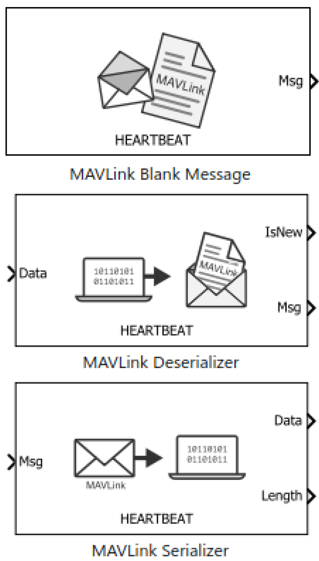
The UAV toolbox in Matlab/Simulink has Mavlink blocks (see Figure 1), which allow for communication with QGroundControl. The first Mavlink heartbeat block from the Figure 1 library was used to select the payload type and data rate for synchronization. The Mavlink serialized block was used to convert the virtual bus message into an unsigned integer 8 bits data stream. The Mavlink de-serializer block can be used when needed to decode Mavlink message data, but in our implementation, Mavlink was used to send data to QGroundcontrol, but there was no need to receive data back, which could be helpful in situations where the path plan is specified directly in QGroundControl.

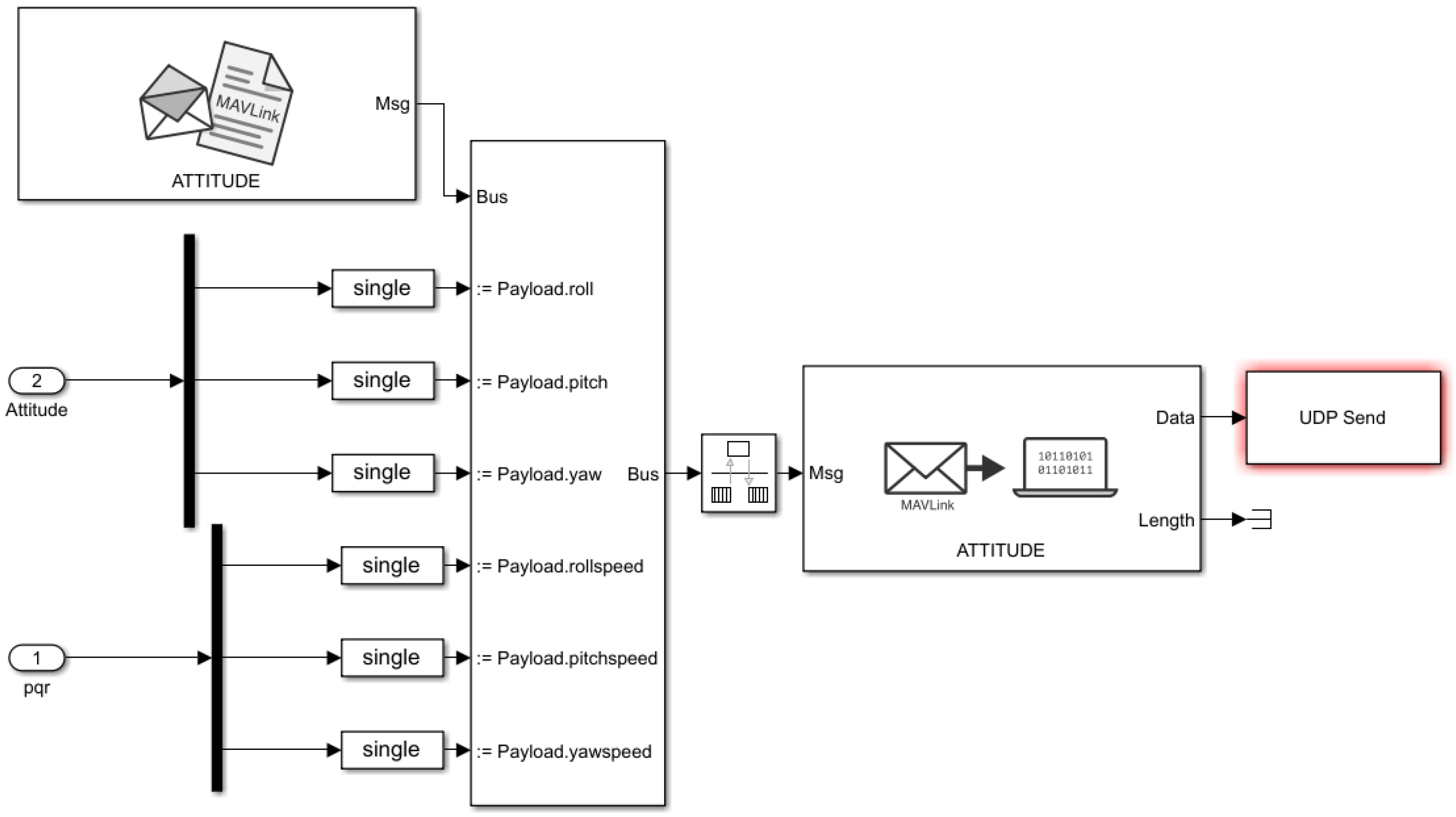
An example of interfacing the attitude and altitude signals in Matlab Simulink with QGroundControl via Mavlink protocol is shown in Figure 2, where the bus assignment block is used to send attitude and angular velocity data as a message payload.

QGroundControl also has a MAVLink Inspector tool in the Analyze Tools menu. All incoming commands for the vehicle are listed in the inspector, which also displays the update frequency, count, and component id of the message, the variable types, and their values in different message fields. The heartbeat message is generally received at a relatively low frequency (typically 1 Hz) compared to sensors such as GPS, which typically operates at 5 Hz to 10 Hz frequencies, and the IMU, which operates at higher frequencies.

5. Implementations of Matlab/Simulink with Xplane and FlightGear

This section describes our own implementation at Coventry University of the Matlab–Simulink co-simulation with Xplane and FlightGear. It is shown that this tool allows for the evaluation of autopilot designs and of some key aircraft flight handling characteristics.

5.1. The Matlab/Simulink and Xplane Co-Simulation

The Xplane co-simulation was taken to be for a conventional Cessna-172 airplane, which is available on Xplane-11. Pitch, altitude, speed, and heading autopilot designs can be implemented in the Matlab/Simulink model, then evaluated and validated using Matlab and 3D Xplane co-simulation.

The initial condition on Matlab was matched with the initial altitude and location in Xplane using the MAP functionality.

The frame rate was taken to be 20 packets per second.

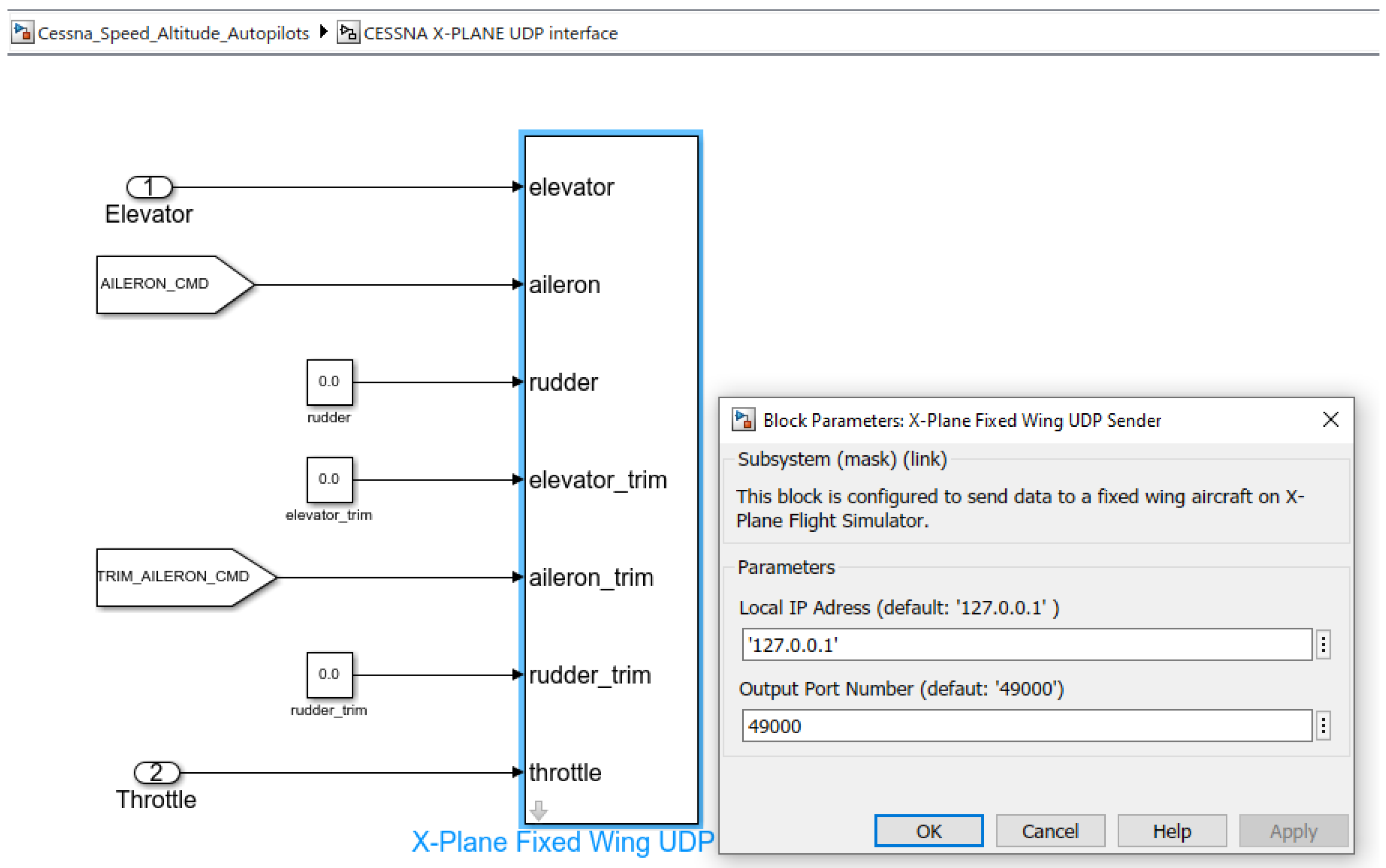
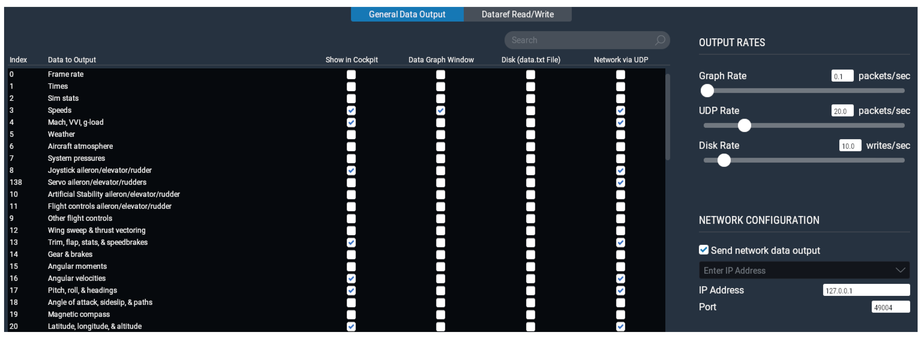
The IP address used for Matlab and Xplane communication via UDP was 1270.0.0.1. The output ports 49,000 and 49,004 were respectively used for Matlab to Xplane and Xplane to Matlab communication via UDP. The UDP send setup on the Matlab side is shown in Figure 3. The UDP setup and inputs and outputs selection are shown in Figure 4.

Wind disturbance can be entered either using Matlab–Simulink or from Xplane, where clear, windy, and even stormy conditions can be simulated at different times of the day. In Matlab, a formal Dryden wind gust model is also available from aircraft autopilot examples.

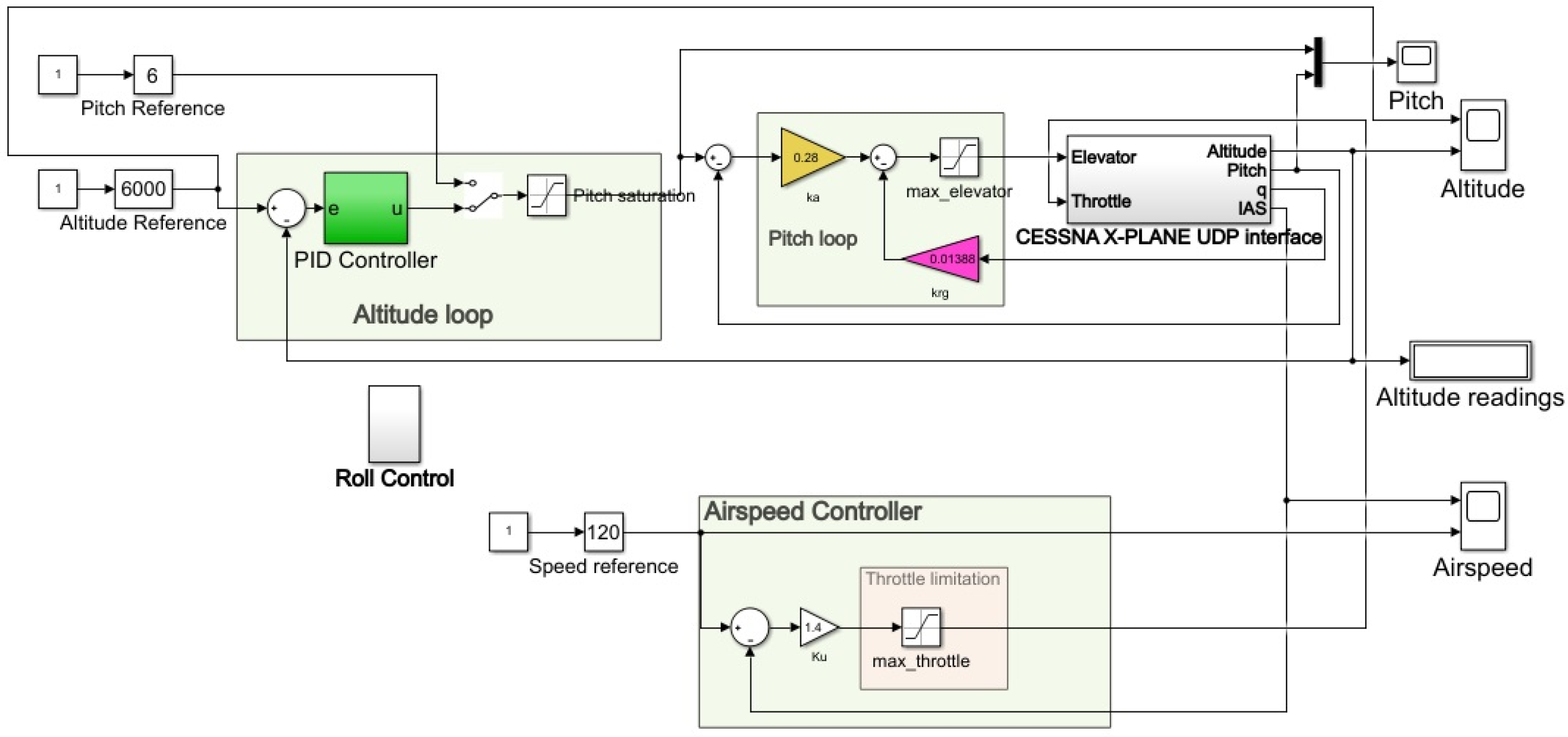
The Simulink altitude and speed autopilots with Xplane interfacing are shown in Figure 5. The altitude control is performed using a conventional successive loop closure approach with a pitch in an inner loop as in [25]. We added a speed autopilot to enable simultaneous speed and altitude control.

More precisely, the following simplified altitude and speed control laws are used:

$${\delta }_e=k_{\theta }\left({\theta }_c-\theta \right)-k_{q}q$$

(1)

where ${\delta }_e$ represents the elevator deflection, ${\theta }_c$ is the desired pitch, $\theta$ is the actual pitch angle, $q$ is the pitch rate and $k_{\theta }$ $, k_q$ are positive controller gains. To track the desired altitude, the desired pitch is given by:

$${\theta }_c=k_h\left(h_c-h\right)$$

(2)

where $h, h_c$ respectively represent the actual and desired altitudes and $k_h$ is an altitude control gain. Likewise, speed control is performed using autothrottle with proportional control.

$${\delta }_{\tau }=k_{\tau }\left(u_c-u\right)$$

(3)

where ${\delta }_{\tau }$ is the throttle lever angle, $u$ and $u_c$ respectively represent the desired and actual axial speeds and $k_{\tau }$ is a positive constant gain. All control inputs are saturated to keep them within an admissible range. Note that the gains may be replaced by proportional plus integral control to add flexibility to the tuning, but we verified that proportional control in all loops is sufficient for constant setpoint tracking.

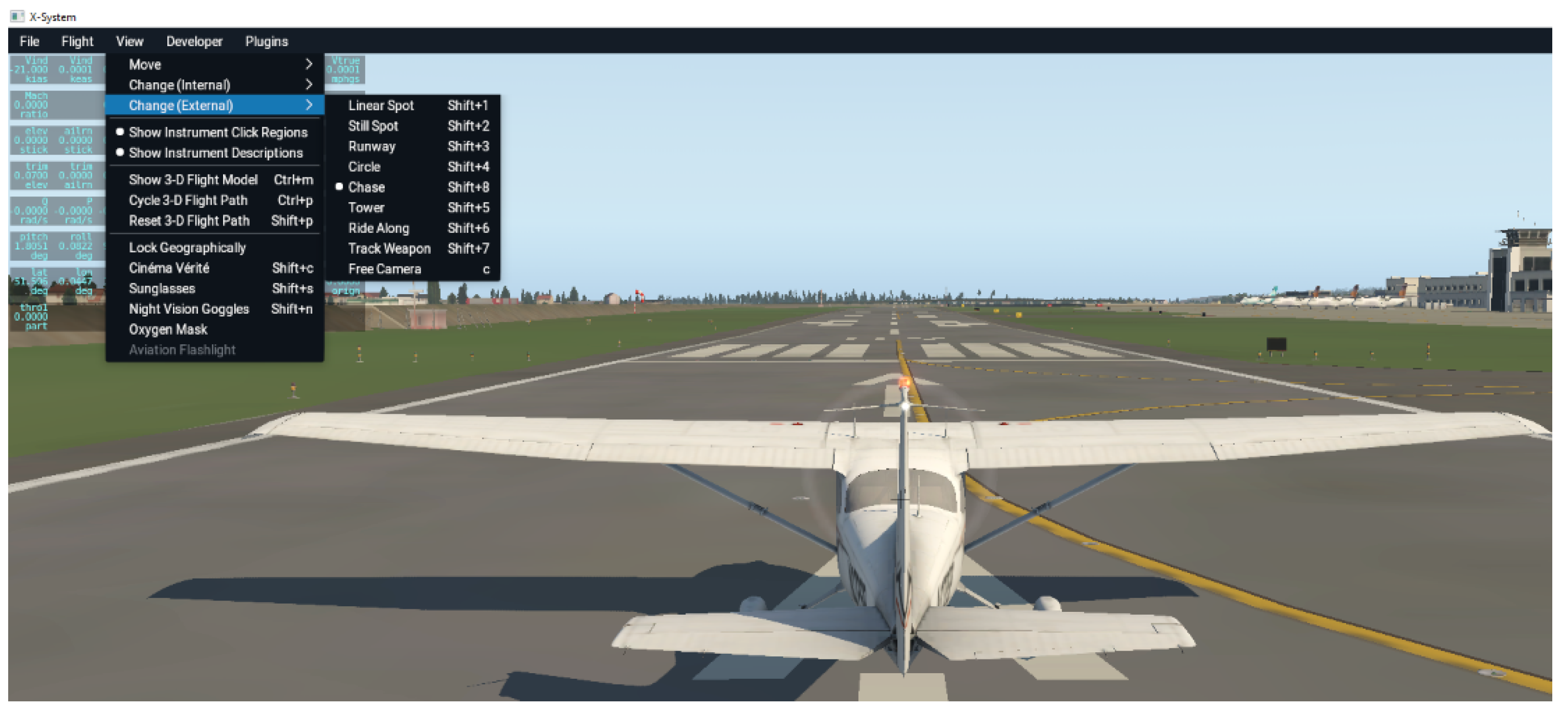
The chase view is selected from the Xplane menu, as shown in Figure 6.

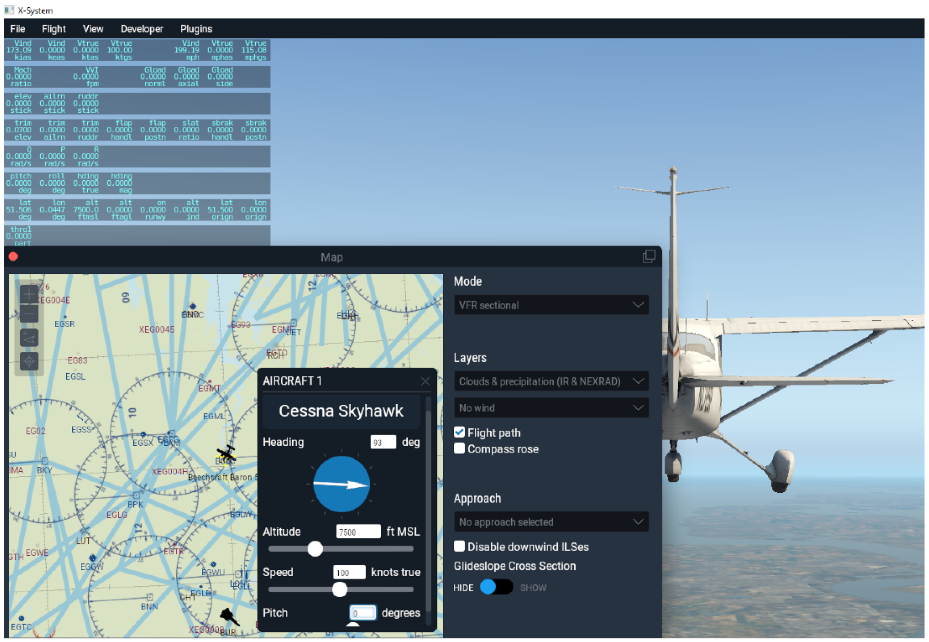
The Xplane map is then selected, and by typing the N key, the map is centered on the aircraft. Once the map is opened, it is then possible to enter the initial altitude and speed of the aircraft, as shown in Figure 7. The initial speed and altitude have to match the one on the Simulink side.

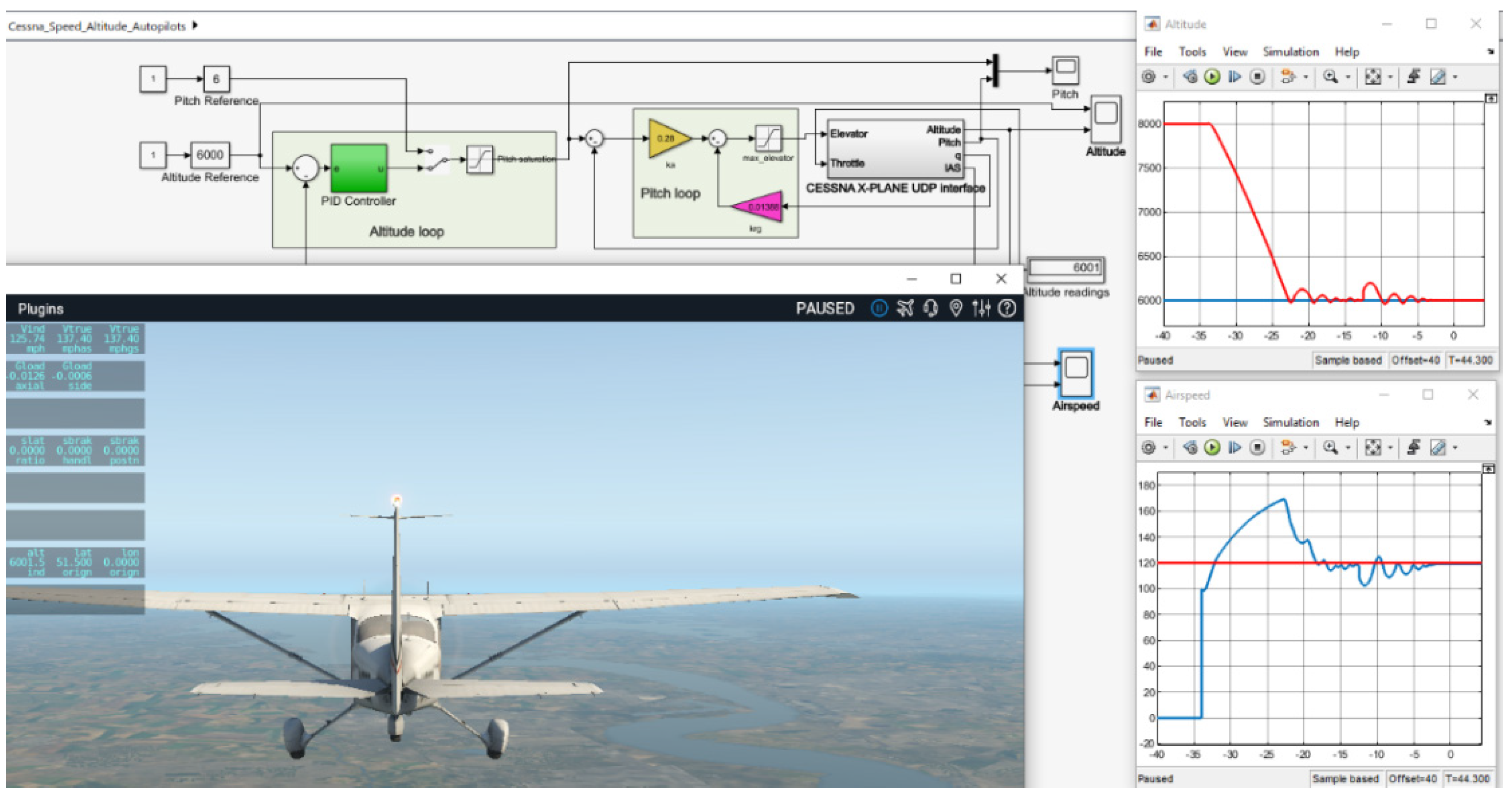
The flight co-simulation is then shown in Figure 8. The aim of this simulation was to simultaneously control altitude and speed reference changes using throttle and elevator inputs while maintaining roll stability. The speed and altitude can be visualized in real-time on the Simulink scopes during the flight and are part of the displayed data on Xplane. The speed and altitude are both controlled to their desired references. The altitude is indeed controlled from 8000 m to the desired altitude of 6000 m in this scenario, and the speed is successfully controlled from 100 to 120 knots. Note that the initial speed of zero in the graphs should be ignored as it just represents the data before giving the aircraft its initial position in Xplane. The Cessna can present challenges to control for an inexperienced pilot because it has a single axial propeller, which causes a yawing moment that needs to be counteracted. That is why a roll control loop was also enabled to avoid roll motion disturbing the longitudinal control.

5.2. The Matlab/Simulink and FlightGear Co-Simulation

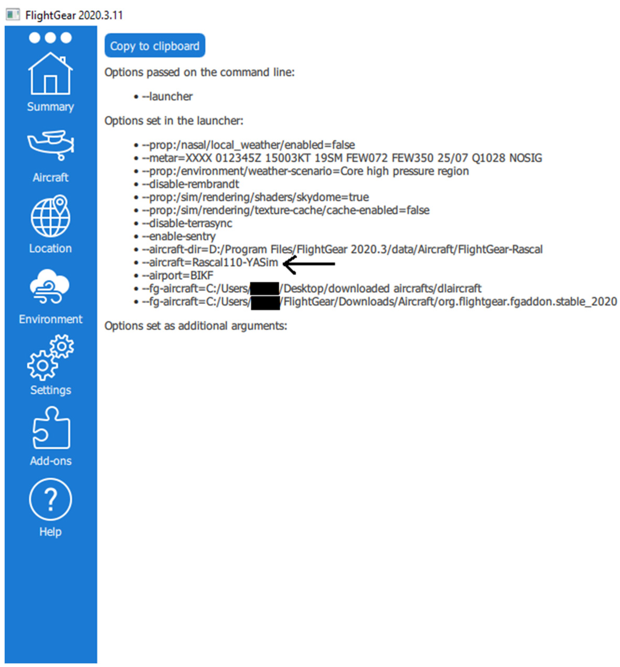
This co-simulation was taken to be for a Rascal 110 fixed-wing small UAV, for which a FlightGear model was developed by Thunderfly Aerospace (available from GitHub). This allows for the description of the process of interfacing with a customized aircraft design. The aircraft design, which consists of a compressed zipped folder, just had to be extracted and installed in the FlightGear 2020.3\data\Aircraft folder. It is important to remove the “-master” part of the filename often generated by GitHub by default. Before generating the batch script, the file name and version of the aircraft installed must be confirmed by launching FlightGear on its own and looking it up in the command window, as shown in Figure 9.

The command window is used to look up the correct aircraft names, currently set options, and other commands that can be passed on to FlightGear by the batch file. The same commands are used in the .bat file itself.

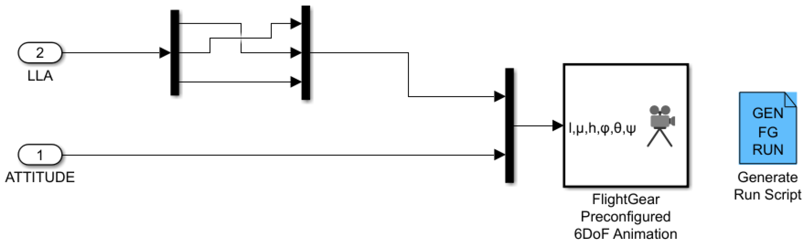
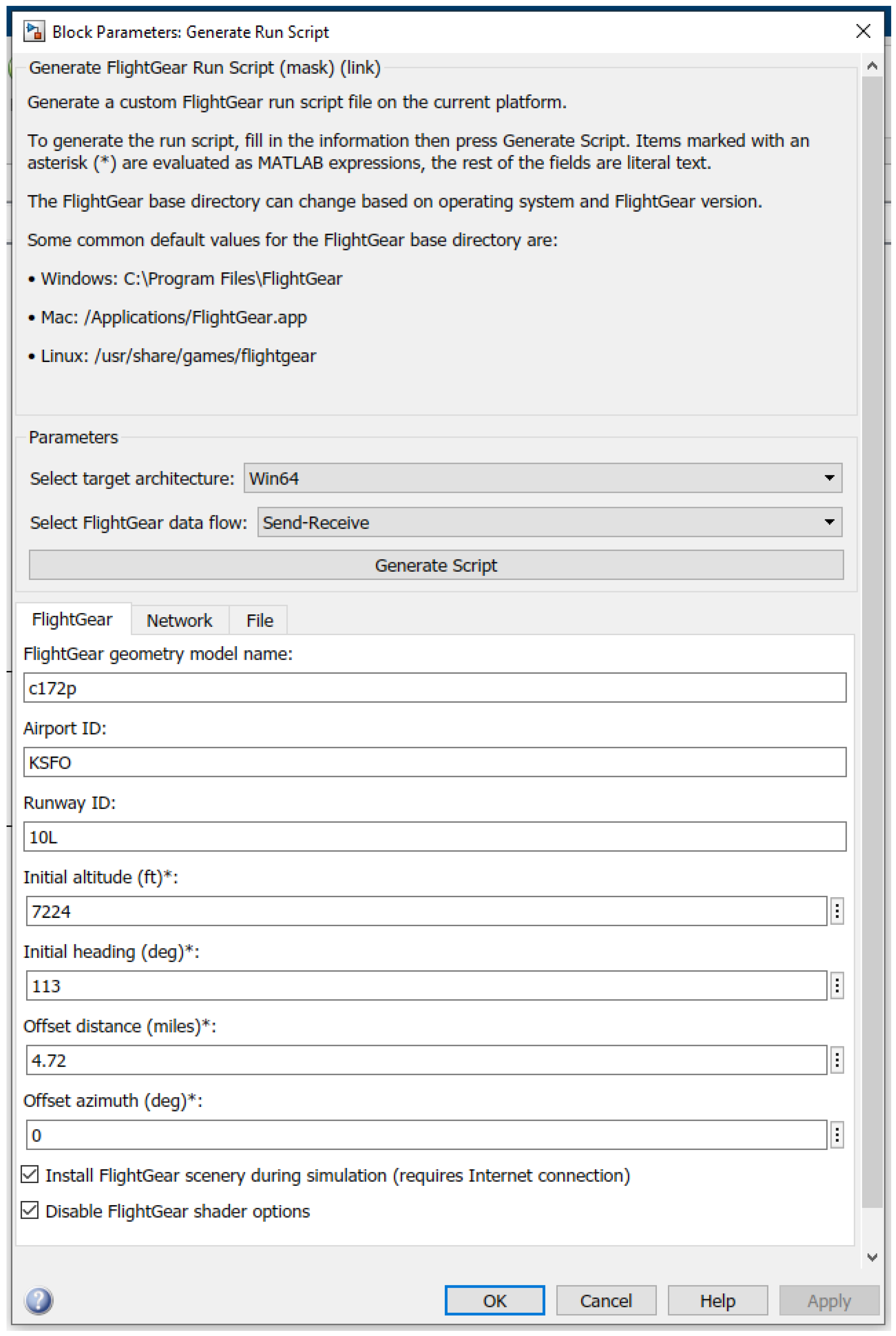
In Matlab, the batch script is generated using a dedicated FlightGear bat file generator block. This block is the blue one shown in Figure 10, and it allows us to select the initial parameters, initial location, aircraft geometry, etc. In our case, no sceneries were pre-downloaded, so the option to install scenery during the simulation was on. Disabling shader options is the recommended choice as it greatly improves the performance of the simulation for machines that are not fitted with high-end graphics cards and CPUs. The parameters of the run script setup from Simulink are shown in Figure 11.

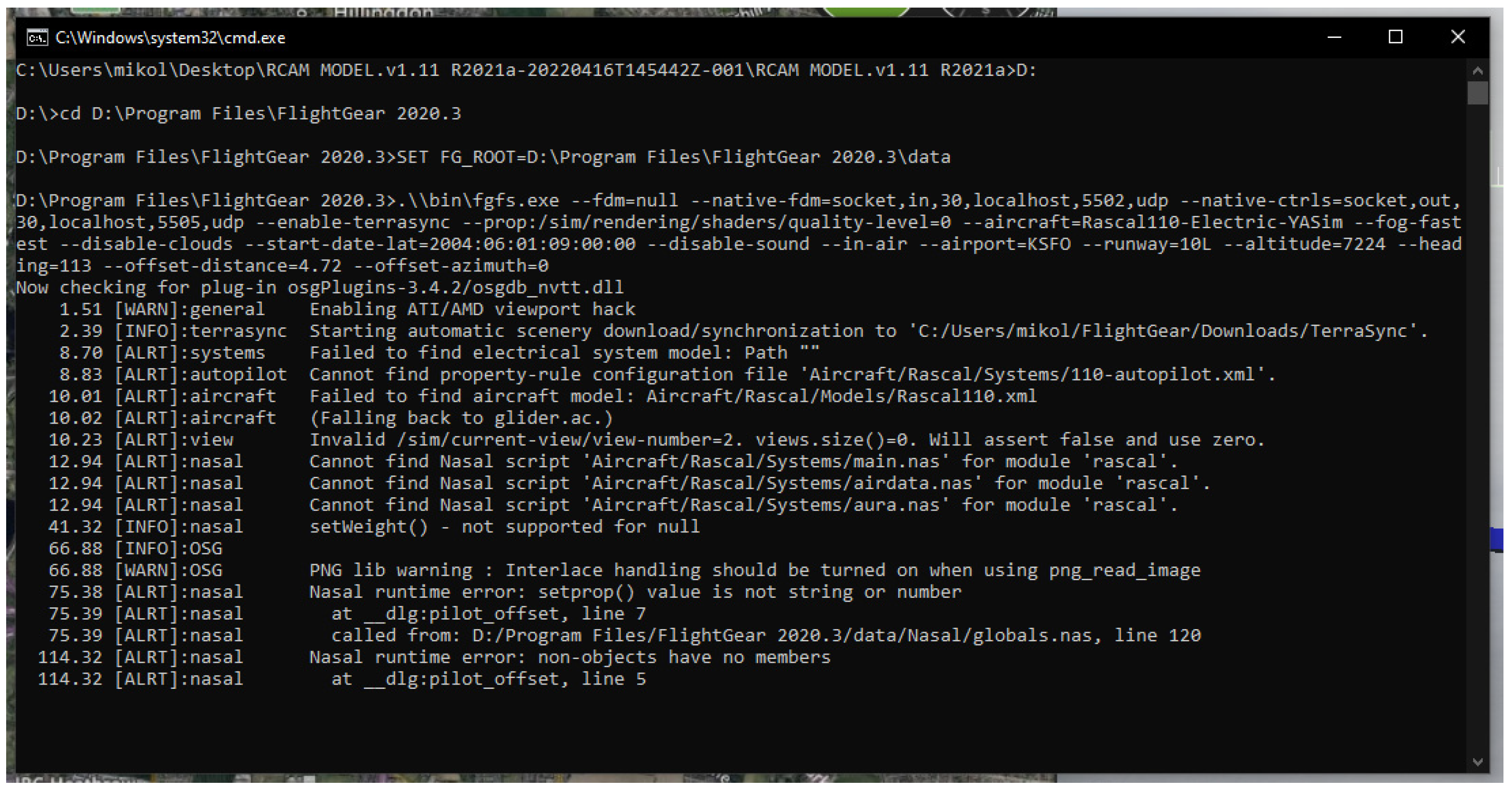
Executing the batch file automatically opens FlightGear with the Rascal UAV, as shown in Figure 12. The software launched that way is prepared to receive data from Simulink. When the simulation is started in Simulink, the UAV starts from the initial condition specified in Matlab.

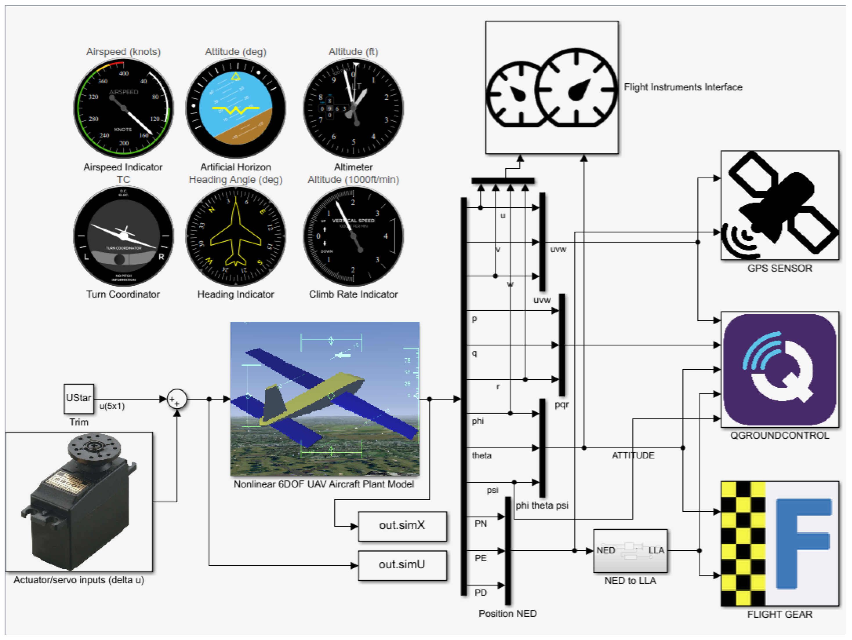
A nonlinear 6DoF model was developed for the Matlab/Simulink Simulink of a Rascal 110 UAV. The model was trimmed using the fminsearch Matlab command with a loss function to minimize the errors in solving nonlinear equations used to trim the model using the process described in [26]. It was then linearized using the linmod Matlab command. The FlightGear block in the simulator model requires longitude, latitude, and altitude (LLA) information as well as aircraft roll, pitch, and yaw angles.

In vector form, the nonlinear dynamics are given by:

$$m({\dot{V}}_{\mathrm{b}}+{\omega }_b\times V_{\mathrm{b}})=F_{\mathrm{b}}$$

(4)

$$J {\dot{\mathsf{\omega }}}_{\mathrm{b}}+{\omega }_{\mathrm{b}}\times J{\omega }_{\mathrm{b}}=m_{\mathrm{b}}$$

(5)

where $V_{\mathrm{b}}$ represents the velocity vector of the aircraft, expressed in body coordinates, ${\omega }_{\mathrm{b}}$ represents the angular velocity vector of the body frame with respect to the inertial frame, $F_{\mathrm{b}}$ represents the resultant external force in the body frame, $m_{\mathrm{b}}$ denotes the moment vector acting on the UAV, m is the UAV mass and J is the moment of inertia matrix. The forces and moments models that relate $F_{\mathrm{b}}$ and $m_{\mathrm{b}}$ to the elevator, aileron, rudder, throttle inputs, and the states of the system were taken and modified from the model developed by Christopher Lum for the RCAM research aircraft, which was originally developed by the Garteur group (see [27]), but the model was modified for the Rascal-110, which has a single central axial propeller. The trim condition $x^{*},u^{*}$ where $x^{*}={\left[V_{\mathrm{b}}{}^{*T},{\omega }_{\mathrm{b}}{}^{*T},{\varphi }^{*},{\theta }^{*},{\psi }^{*}\right]}^T$ is the state vector and $u^{*}$ is the trimmed control inputs vector was computed by minimizing the quadratic error cost function $J={\dot{x}}^{*T}{W}_1{\dot{x}}^{*}+{\dot{u}}^{*T}{W}_2{\dot{u}}^{*}$, where ${\varphi }^{*},{\theta }^{*},{\psi }^{*}$ are trim conditions on the roll pitch and yaw angle and $W_1$, $W_2$ are diagonal weighting matrices that are used for numerical conditioning and are typically multiples of the identity matrix. Minimizing the cost function leads to the equilibrium condition ${\dot{x}}^{*}={\mathbf{0}}_{\mathbf{9}\times \mathbf{1}},{\dot{u}}^{*}={\mathbf{0}}_{\mathbf{4}\times \mathbf{1}}$. The four components of the control vector $u^{*}=\left[{\delta }_e^{*},{\delta }_a^{*},{\delta }_r^{*},{\delta }_t^{*}\right]$ respectively represent the trimmed elevator, aileron, rudder, and throttle commands. The Simulink model is shown in Figure 13. Note that for Matlab versions 2021A or earlier, the GPS sensor should not be used. The operating condition for the simulation was a trim speed of 85 m/s with an altitude of 1000 m. Flight testing for this model consisted of manual control inputs with elevator inputs between −10 degrees and 25 degrees, throttle inputs between 0.5 degrees and 10 degrees, aileron inputs between −25 degrees and 25 degrees, and rudder inputs between −30 degrees and 30 degrees to validate the aircraft responses for nine state variables, namely the axial, vertical and lateral speeds, the attitudes and angular rates on all three axes.

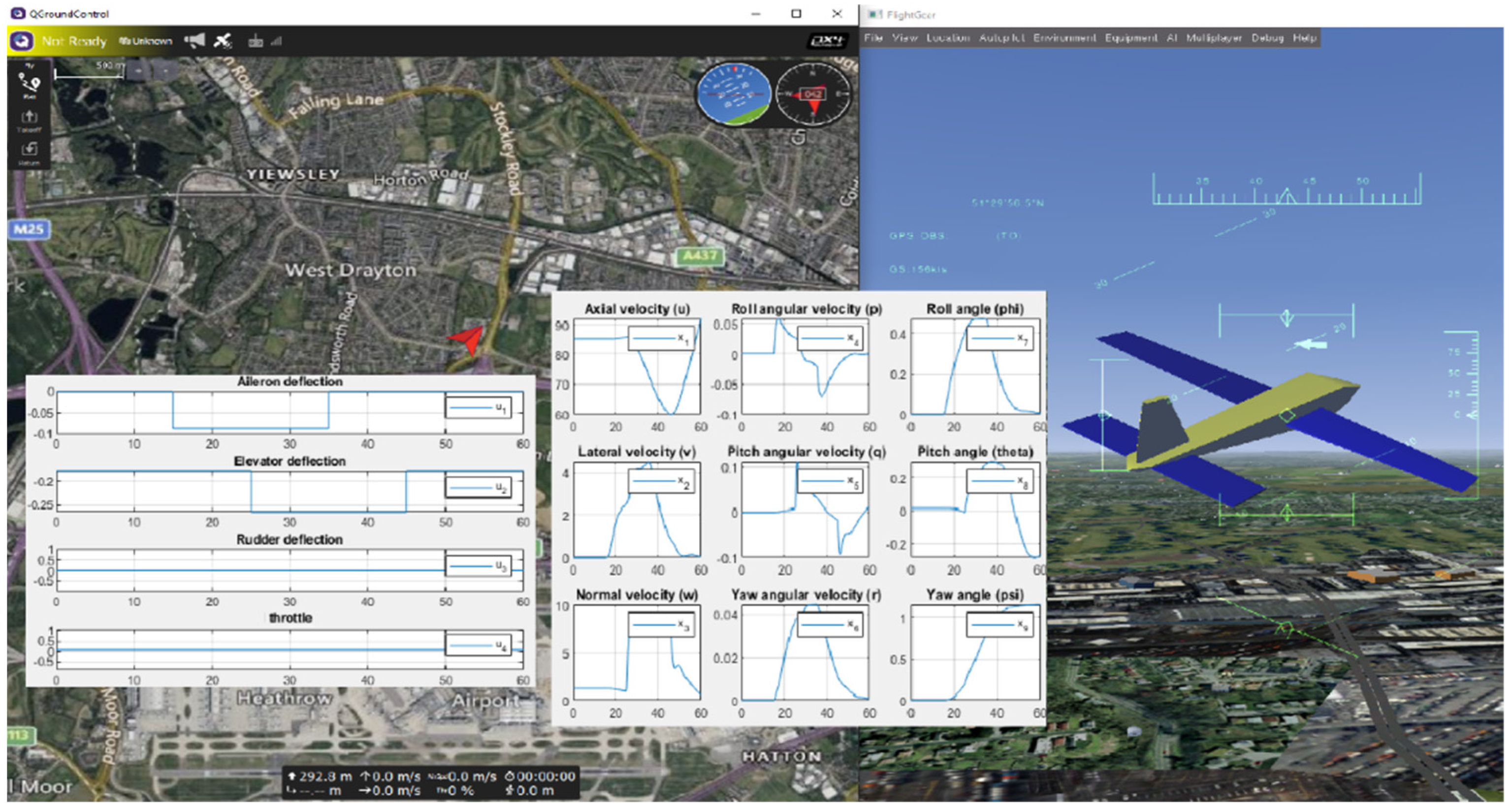
The 3D simulation obtained by interfacing Matlab/Simulink with FlightGear via UDP is shown in Figure 14 for an open loop maneuver using a 6DoF nonlinear UAV dynamical model, which was developed in Simulink with FlightGear for 3D visualization.

6. Software-in-the-Loop Co-Simulation Using Matlab/Simulink and VFTE

Two approaches are described for SIL and HIL simulation using Matlab/Simulink. The first one is based on the UAV toolbox for PX4, and the second one is based on a co-simulation using Matlab/Simulink with flight simulation software, which is taken in this section to be the Alphalink virtual flight simulation environment (VFTE) without loss of generality.

6.1. UAV Toolbox for PX4

Matlab’s UAV Toolbox Support Package for PX4^® allows for the use of Matlab/Simulink for SIL but also HIL simulation with small UAV NuttX-based autopilots, including the Pixhawk autopilots family. After installing the toolbox, it is necessary to set it up to work with a chosen hardware board using the configuration parameters options. The toolbox also has libraries allowing different types of connections for the key aircraft sensors, including inertial navigation sensors (INS), global positioning system (GPS) receivers, speed pressure sensors, servo actuation for the control surfaces and DC motors, battery monitoring, and other features. 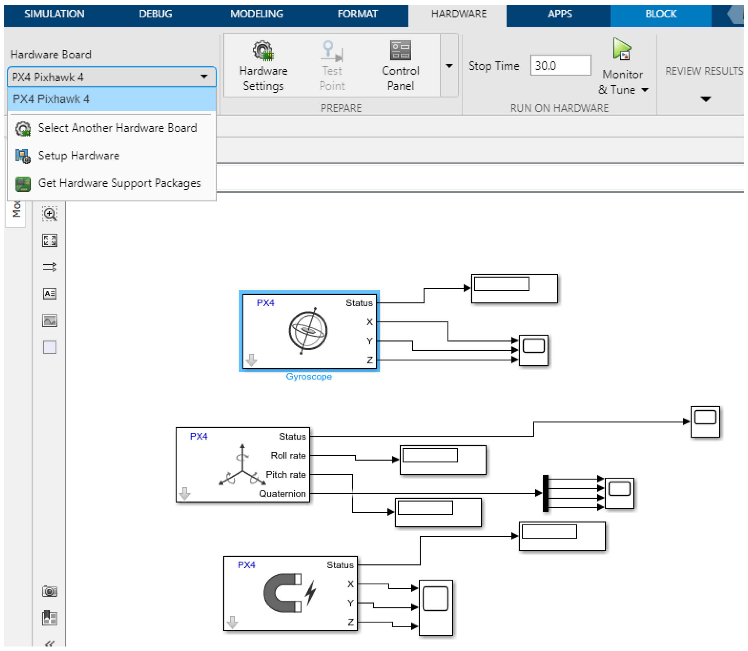Figure 15 shows the Matlab/Simulink layout for a simple model used for initial sensor testing, and the HIL testing of the sensors and gyros is simply started by clicking on Monitor and Tune. Example models are also provided by Matlab to allow for gyro sensor calibration to remove bias and scaling errors, for example.

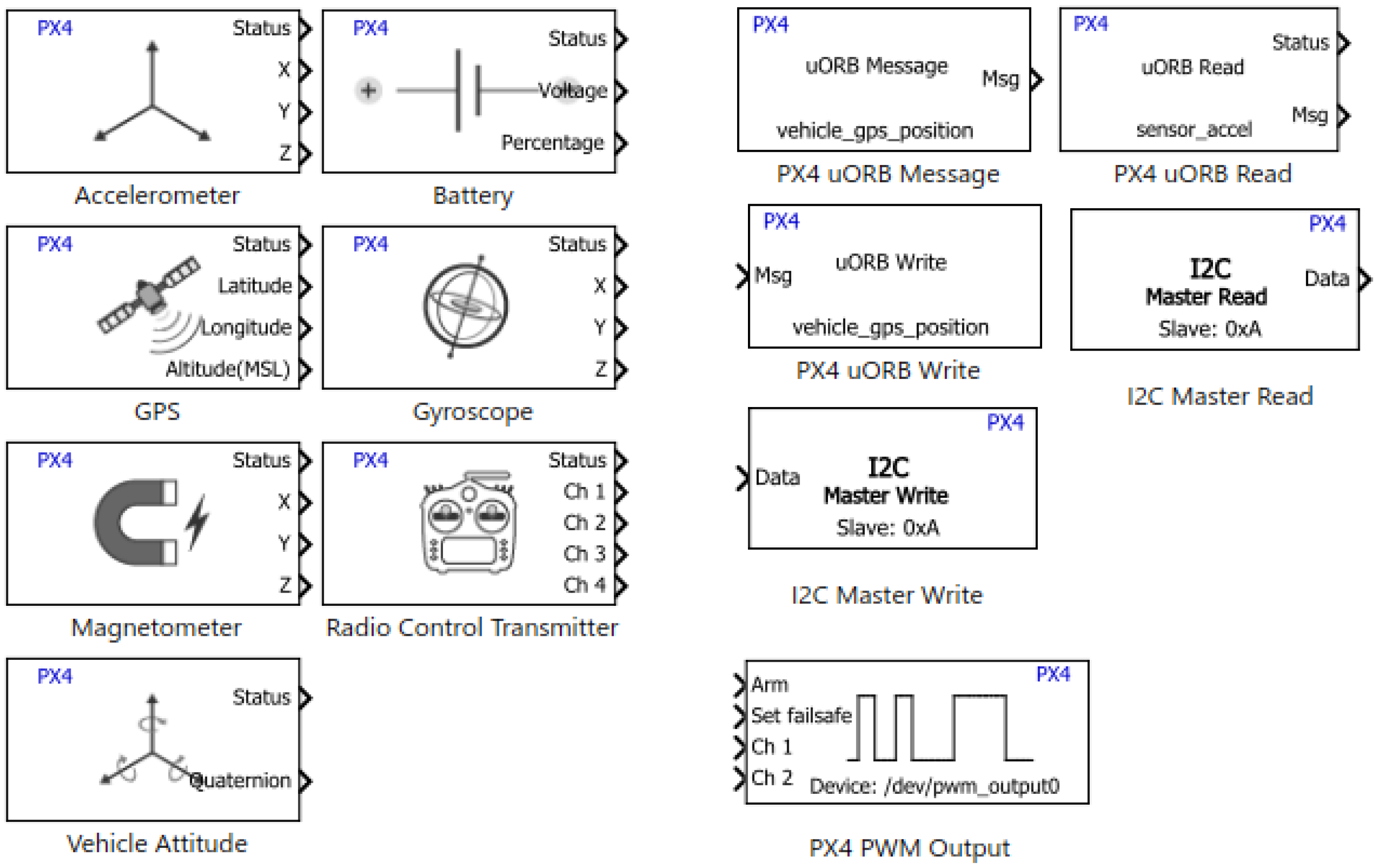
The toolbox also provides libraries for the uORB asynchronous publish/subscribe messaging system. This middleware allows components to publish data about a topic, such as gyro readings, and other components to receive messages by subscribing to the corresponding topics. Additional generic uORB read and write blocks are also provided to add flexibility, such as defining new or combined topics using Simulink bus assignment blocks. The libraries of the UAV toolbox for PX4 are shown in Figure 16. The uOrb blocks can be used in both SIL and HIL modes of operation.

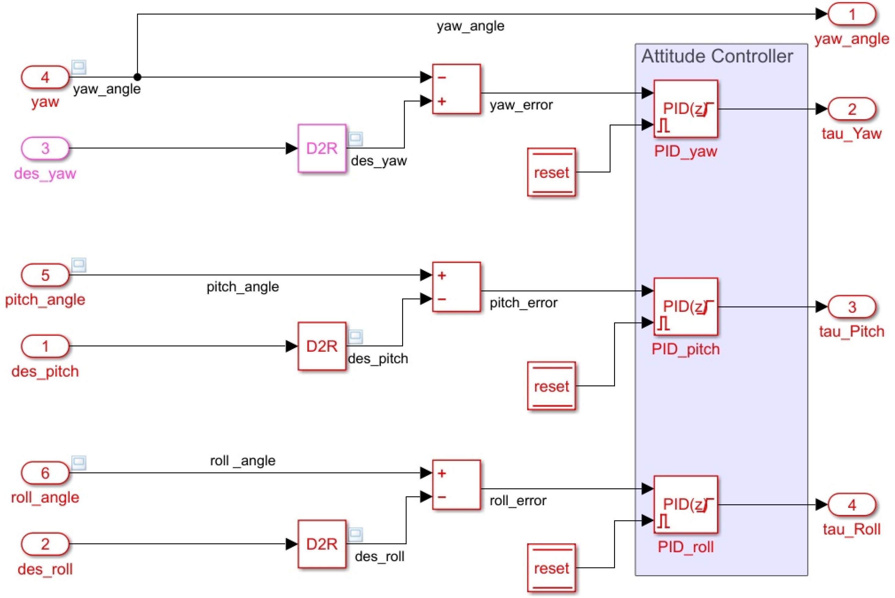
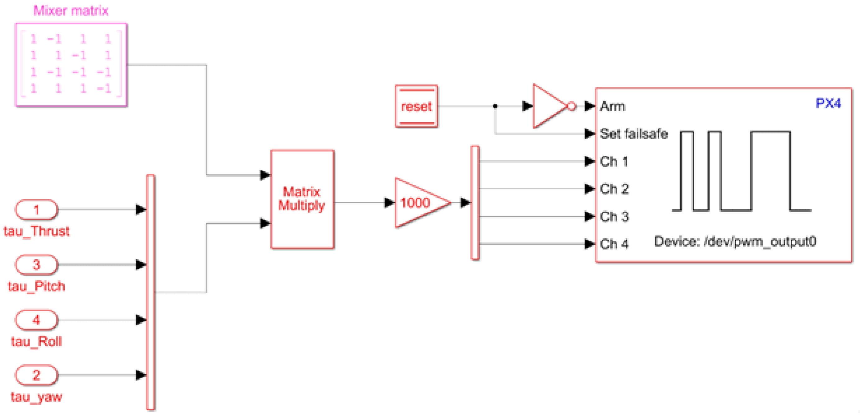
SIL simulation is possible using the Pixhawk host target option under the hardware setup instead of an actual Pixhawk board. Several SIL example models are provided by Mathworks. In [28], a SIL example is provided for the position tracking of an X-configuration quadcopter. This SIL simulator allows for the evaluation of autopilots through 3D simulation using the jMAVSim flight simulator. Conventional roll, pitch yaw, and altitude autopilots are used. The block diagrams of the autopilots and control allocation/mixing are shown in Figure 17 and Figure 18, respectively.

To deploy custom flight controllers or navigation algorithms from Simulink to the Pixhawk boards, it is necessary to suppress the execution of certain startup processes and to force the autopilot to run the Simulink model. This is performed by using a startup script, which is copied to the micro-SD card to be mounted on the Pixhawk^® Series flight controllers. This requires the installation of the Embedded Coder^® Support Package for PX4 Autopilots.

In [29], a Pixhawk-4-based quadcopter HIL simulation model is provided as a Mathworks example. The PX4 firmware is configured using QGroundControl for HIL simulation. UDP interfacing is used for communication with QGroundControl and with a 3D scene simulation using Unreal Engine, which has particularly good scene rendering in a city environment. The dynamical model is implemented in Simulink with Mavlink bridge sink and source blocks to communicate with the Pixhawk 4 autopilot as well as QGroundControl and the 3D scene simulation, as shown in Figure 19. Actuators and sensors are, however, not used in this example. For actual flight, the flight controller program can still be used but without the dynamical model. The PX4 firmware would have to be configured for real flight, and the Pixhawk 4 connections to the propellers would have to match the one assumed in the SIL simulation.

6.2. SIL Simulation Using Matlab/Simulink and VFTE

In this section, we present one example of SIL implementation using Matlab/Simulink together with the VFTE Nano Talon UAV simulator, taken and adapted from Alphalink training resources. The control objective is simultaneous roll and yaw control, with robustness to disturbances such as the sideslip disturbance due to the wind. Roll and yaw motions are well known to be coupled in fixed-wing aircraft. The inputs and outputs of this SIL model are very similar to those of the Alphalink-based HIL flight simulation, but sensors and actuators are both virtualized.

More details about the ZOHD Nano Talon UAV and its use as a flying lab is presented in [30]. The UAV has a 0.86 m wingspan and a length of 0.57 m. A pusher prop with a maximum thrust of 425 g is used for axial propulsion. Yaw and pitch control is performed using a twin rudder. Conventional control mixing is used to derive the required right and left rudder inputs for pitch and yaw control.

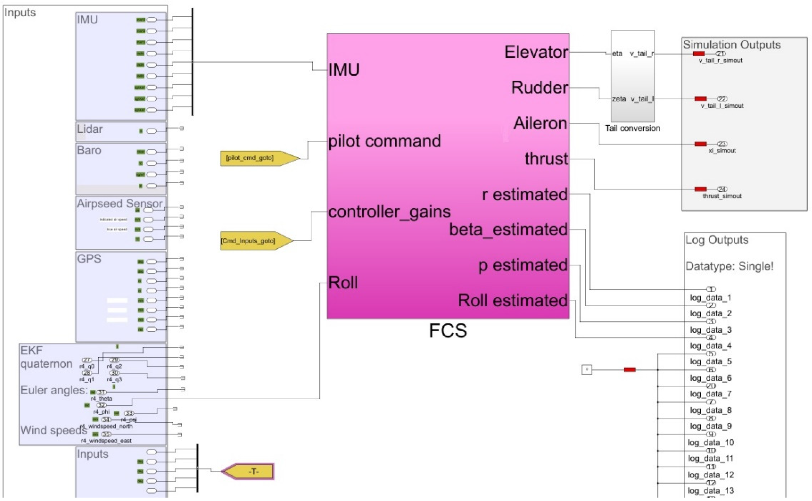
The Simulink model template for VFTE interfacing has multiple inputs that can directly be used from the sensors (IMU, GPS, pitot tube, lidar), and attitude estimates are also available from an extended Kalman filter input as shown in Figure 20, where roll angle feedback is obtained from the EKF using simulated sensor readings in the case of SIL and HIL. A very similar model is also available for flight testing, with the key difference that actual sensor readings are used instead of simulated ones. For both SIL and HIL simulations, all control inputs can be sent to the four actuators onboard the Nano Talon UAV, namely a ruddervator with mixing from elevator and rudder commands, an aileron command, and a throttle input. Wind inputs can easily be injected into the flight simulation using either using Simulink or directly using the VFTE flight simulator.

A robust mixed sensitivity H-infinity controller is used by calling Matlab command mixsyn in a Matlab script that is executed to generate the model and controller parameters before running the Simulink model. The H-infinity state feedback places the poles to minimize a weighted cost function that ensures a weighted tradeoff between disturbance rejection (sensitivity function dependent), reference tracking (complementary sensitivity function dependent), and energy consumption. The robust optimization problem that is solved using mixsyn can be formulated as:

$$\underset{K\left(s\right)}{\min }{\parallel \begin{array}{c}{W}_{s}S\left(s\right)\\ \begin{array}{c}{W}_{KS}K\left(s\right)S\left(s\right)\\ W_{T}T\left(s\right)\end{array}\end{array}\parallel }_{\infty }$$

(6)

where S is the sensitivity function from low-frequency disturbance to output and T is the complementary sensitivity function from reference to noisy output. S needs to be minimized at low frequencies, and T needs to be minimized at low frequencies, and the two conditions cannot both be satisfied at the same frequency because S + T = I. The conditions in one frequency domain are, however, compatible because, at low frequencies, T has to approach identity to ensure reference tracking. S and T are 2 × 2 matrices.

The controller transfer function K (s) takes sideslip and bank angle data as inputs and outputs the aileron and rudder deflections. In the SIL example of Figure 17 and Figure 18, given that high-frequency IMU noise is filtered, $W_T$ is taken to be zero to focus on wind disturbance rejection and reference tracking, but noise rejection can also be explicitly accommodated if necessary using the same H-infinity commands. The $W_s$ matrix is diagonal with a low-frequency gain of 60 dB for disturbance rejection in both the aileron to roll and the rudder to yaw loops.

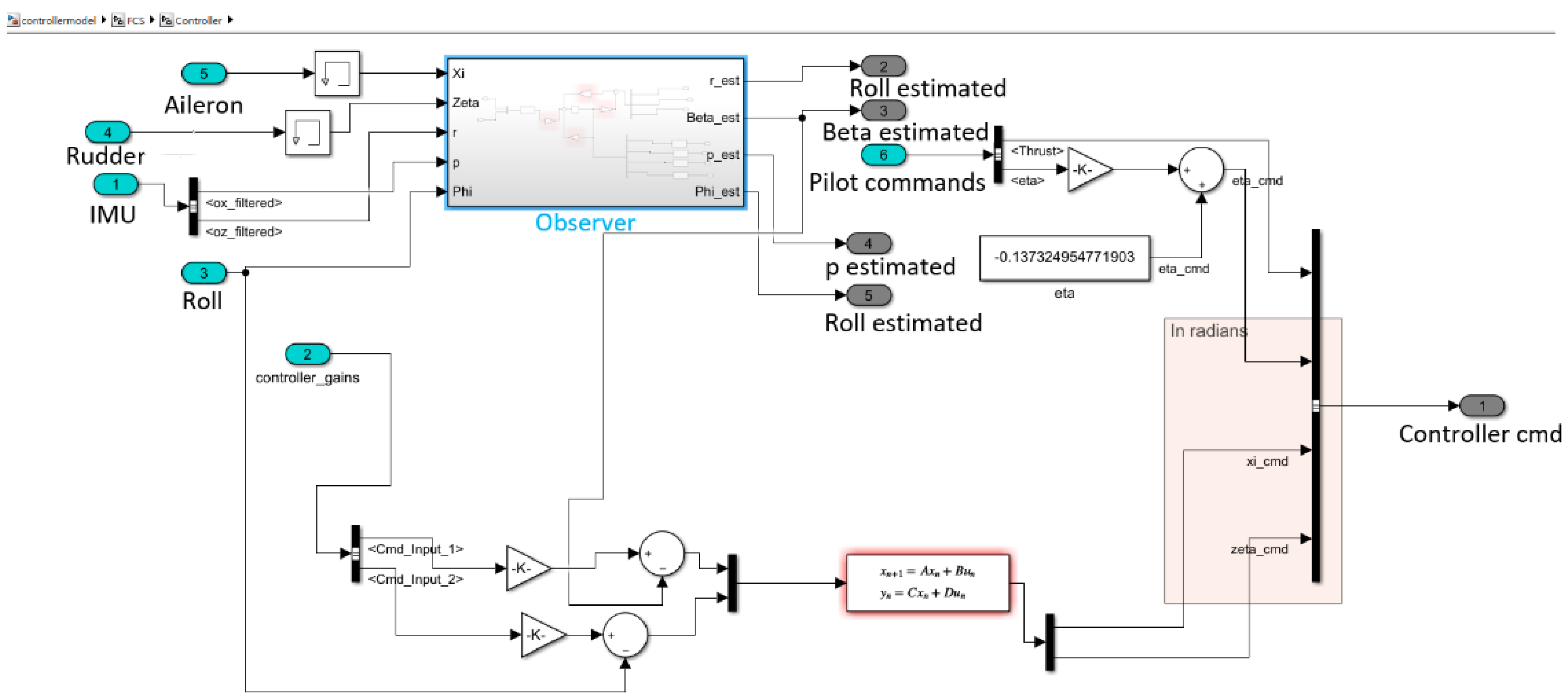
A Luenberger observer is also used, as shown in Figure 21, to provide the required state feedback for the lateral controller because the sideslip angle is not directly measured, unlike the roll, roll rate, and yaw rate. The full detail of the observer block and the H-infinity function is not provided here because they were modified from a commercially available Simulink/VFTE simulation lesson by Alphalink Systems plc. Angular rate information is obtained from the simulated Pixhawk gyros with low pass filters to reduce the effects of noise. The bank angle feedback is directly obtained, as shown in Figure 17, from an extended Kalman filter (EKF), which is available by default as PX4 code.

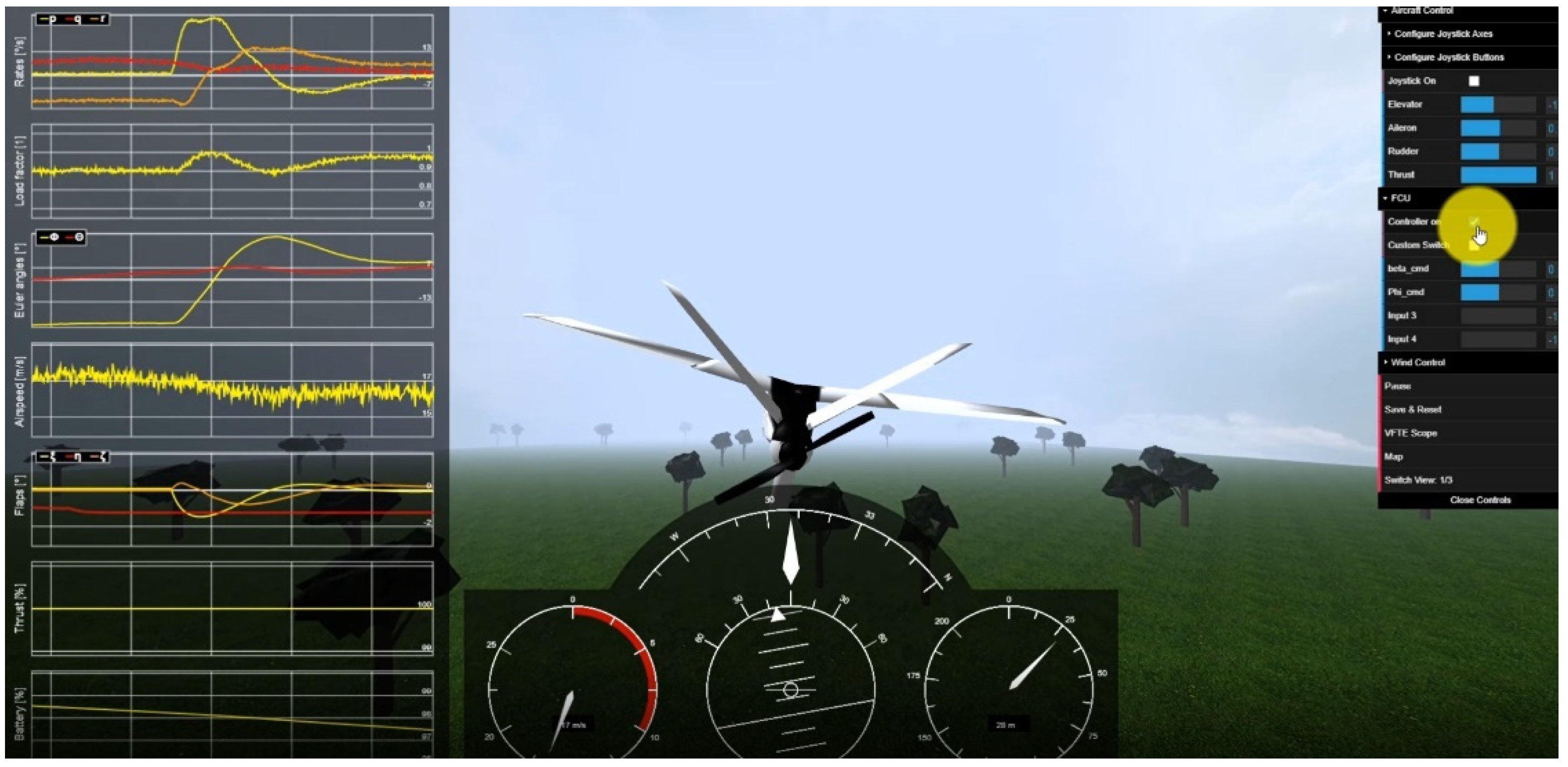
The VFTE window during the Simulink-VFTE flight co-simulation of the observer enhanced lateral control of the Nano Talon UAV is shown in Figure 22. The Nano Talon self-stabilizes after a bank angle maneuver to change the heading and is robust to bounded wind velocities.

The trim condition for the simulation was an axial speed of 17 m/s at 100 m altitudes with the correct angle of attack and throttle settings to maintain that speed constant without a turn.

6.3. HIL Simulation of A Small UAV Using Matlab/Simulink, VFTE, and CAN Interfacing

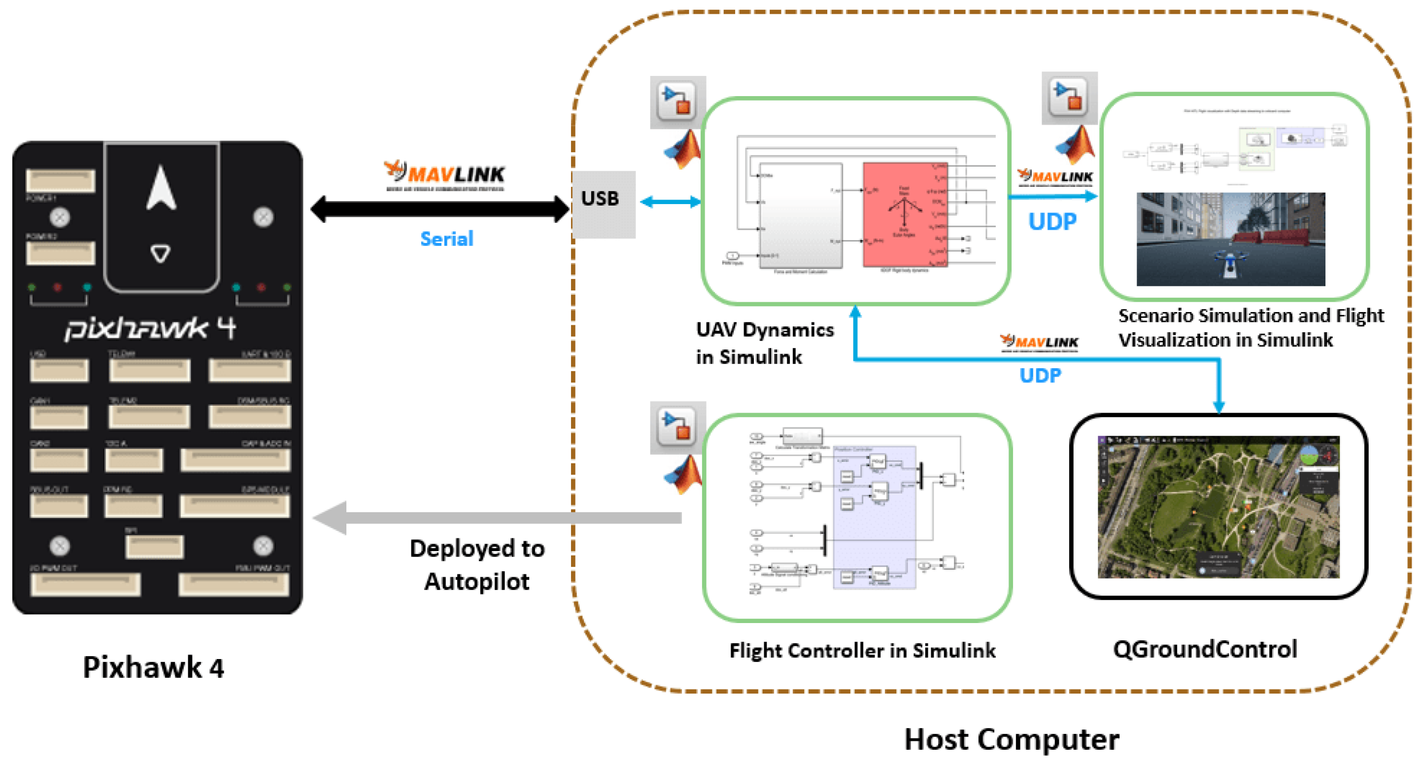
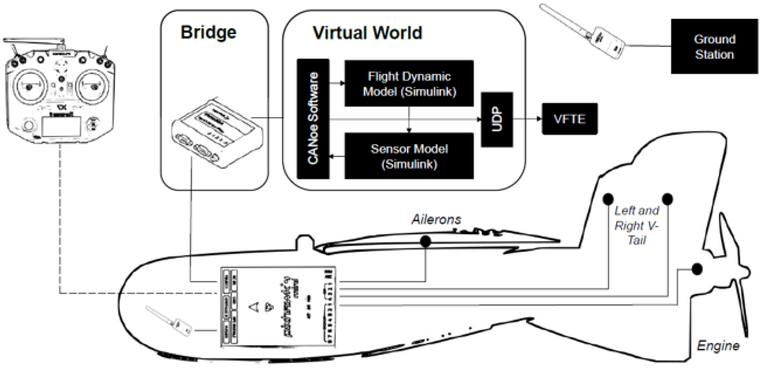
Alphalink’s VFTE was also successfully used for a HIL co-simulation with Matlab/Simulink and QGroundControl for a virtual flight test using the ZOHD Nano Talon UAV. The HIL architecture is shown in Figure 23 and uses a controller area network (CAN) bridge (configured and tested using the CANoe software) to connect the Pixhawk 4 mini flight controller on the one hand and Matlab Simulink dynamical and sensor models on the other hand. VFTE is also interfaced with Matlab/Simulink for real-time 3D flight simulation, and the Pixhawk-4 mini is connected to all the onboard sensors and actuators of the Nano Talon UAV, as well as an RC transmitter. For HIL simulation, a VMwareplayer virtual machine is used to represent the virtual world and upload the flight controller code to replace actual sensor measurements with virtual measurements.

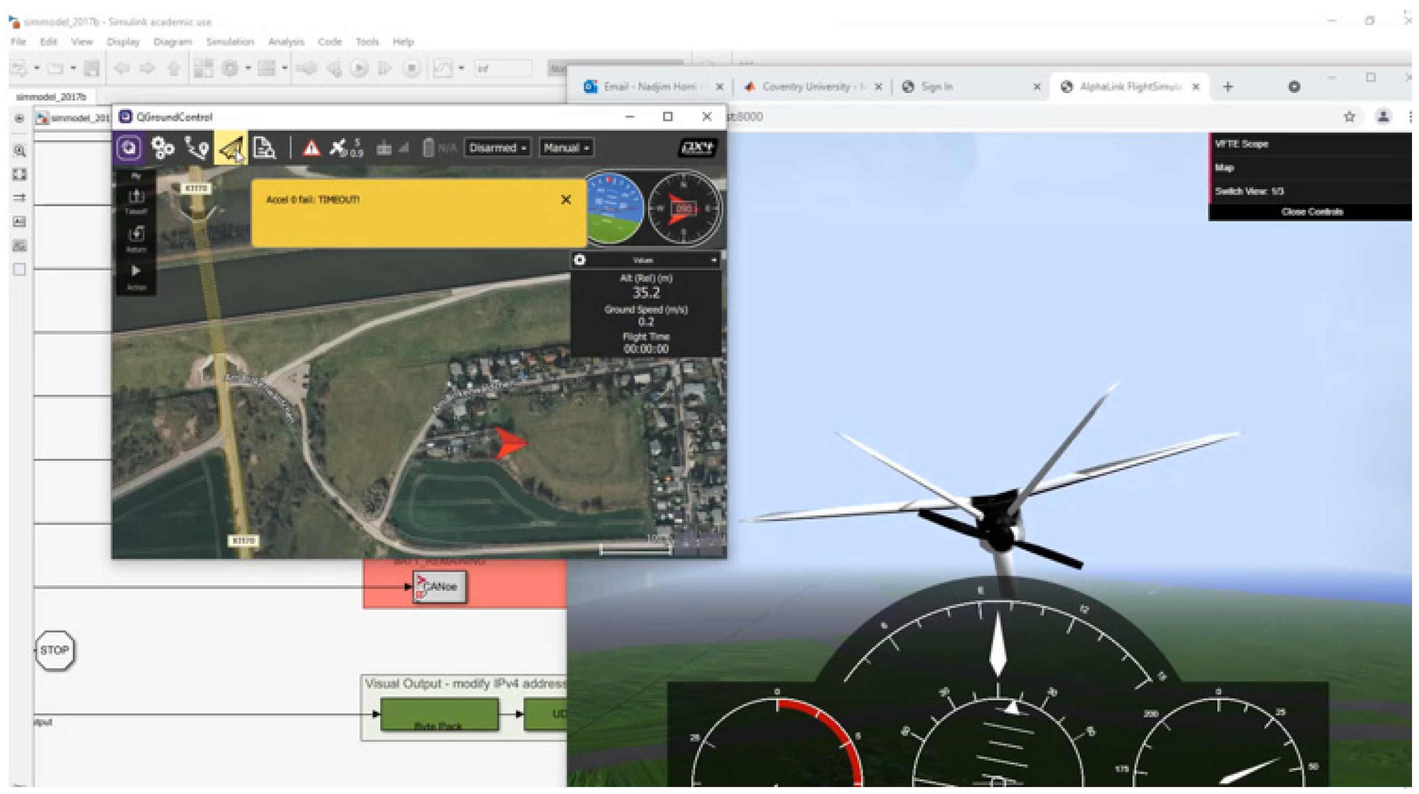
A screenshot of the working Nano Talon virtual flight test excitation of all 6DoF using manual RC transmitter commands to the HIL simulation using VFTE-Simulink and QGroundControl is shown in Figure 24. The servos connected to the Pixhawk were activated during this experiment. This setup would allow for a practical comparison of energy consumption between different control methods, although the power readings would be without the aerodynamic load that would be present in real flight tests. It is, however, still possible to relate power consumption without load to the one with a speed-dependent aerodynamic load through propeller thrust measurement in wind tunnel experiments, which would allow predicting the expected difference between real flight and HIL flight test.

For autonomous control, a similar approach can be used to the SIL setup in Figure 17. As part of the future work, we are developing autonomous longitudinal feedback control of the Nano Talon using a wind perturbation observer for adaptive control in the presence of wind gusts, assuming that there are insufficient measurements to directly measure the wind gusts and their angular rate effects. The Alphalink Nano Talon kit is also capable of flight tests, but the HIL setup allows for improved flight safety through virtual flight tests before real flights. HIL evaluation of power consumption is also possible but will not include the aerodynamic load effects. Model-based corrections would be needed to evaluate the corresponding power fraction under the simulated aerodynamic loads.

7. Discussion of the Limitations of Co-Simulation Methods

The co-simulation methods used in this paper employ commercial software, including Matlab/Simulink by The Mathworks Inc., Alphalink’s VFTE, and Xplane. Matlab script was found to work on all attempted recent Matlab versions, and it is noteworthy that some Simulink toolboxes features, such as those of the UAV toolbox, will only work in the latest Matlab versions (The GPS block in Matlab 2021a or later, for example) and when using a new Matlab version, it is can be necessary to make modifications to the models developed in earlier versions before they can be used. Using Xplane, additional features are available using the professional version of the software, and plugins may be necessary to extend the work to more complex simulations such as formation flight. The Alphalink software is currently specific to the NanoTalon UAV, and SIL/HIL simulations can, in this case, be interfaced with a realistic flight simulation, which is remotely accessed on the cloud, although this did not present any issues in terms of real-time flight simulation, and it has the advantage of using less onboard PC resources for the flight simulation. Real-time flight co-simulation was found to work efficiently on one PC with a moderate capability of 8 GB RAM and a 1.8 GHz intel quad-core processor, with sufficient hard disk memory to run Xplane–Matlab, VFTE–Matlab, or FlightGear–Matlab co-simulations from the same PC.

8. Conclusions

A review on the use of Matlab/Simulink with a range of popular flight simulation programs has highlighted that different PC-based flight simulators have different areas of strength in terms of 3D simulation.

Commercial software Xplane was found to provide a relatively simple approach to real-time co-simulation via UDP with a realistic flight dynamics model based on blade element theory for a wide range of aircraft configurations, but it was primarily designed for manned aircraft. The Simulink–Xplane co-simulation approach was found to be particularly suited to general aviation aircraft and was successfully used to verify the simultaneous altitude and speed control characteristics of a Cessna-172 aircraft, where roll stabilization was also used to counteract the yawing moment due to the use of a single propeller.

Free software FlightGear was shown to allow for flexibility in the choice of the flight dynamics model, with the ability to simulate medium to high endurance UAVs. FlightGear A Rascal-110 UAV was therefore chosen as a FlightGear example. FlightGear was found to provide simple interfacing with ground control station software QGroundControl, which is particularly convenient for path following. A step-by-step tutorial is given to describe the co-simulation process for both Xplane and FlightGear.

Despite the fact that Realflight is well-suited for small UAV simulation, little information is available on its direct interfacing with Matlab/Simulink, and that is why the VFTE software was evaluated for co-simulation in the small UAV case. Approaches to the software-in-the-loop and hardware-in-the-loop flight simulation using Matlab/Simulink are also described using the UAV toolbox or by interfacing Simulink with the VFTE software for virtual flight testing of a Nano Talon MAV. The approach also allows for direct interfacing between Matlab/Simulink and QGroundControl during flight co-simulation in three-dimensional space and for more advanced observer-based robust H-infinity control to optimize a tradeoff between wind disturbance rejection and trajectory tracking accuracy.

The interfaces and conditions for software-in-the-loop virtual flight testing are becoming increasingly similar to hardware-in-the-loop implementation, particularly in the case of small UAVs using tools such as the VFTE or the Pixhawk host target option of the UAV toolbox for PX4. Co-simulation is now becoming the norm for both SIL and HIL testing, particularly in small UAVs where the Mavlink protocol is used, and the trends are towards increased interfacing simplicity.