Article

Analysis and Multiobjective Optimization of a Machine Learning Algorithm for Wireless Telecommunication

1
Computer Science and Engineering Department, University of Quebec in Outaouais, Gatineau, QC J9A 1L8, Canada
2
Energy, Mining and Environment Research Centre, National Research Council, Ottawa, ON K1A 0R6, Canada
*
Author to whom correspondence should be addressed.
Telecom 2023, 4(2), 219-235; https://doi.org/10.3390/telecom4020013
Submission received: 22 February 2023 / Revised: 6 April 2023 / Accepted: 10 April 2023 / Published: 17 April 2023

Abstract

:
There has been a fast deployment of wireless networks in recent years, which has been accompanied by significant impacts on the environment. Among the solutions that have been proven to be effective in reducing the energy consumption of wireless networks is the use of machine learning algorithms in cell traffic management. However, despite promising results, it should be noted that the computations required by machine learning algorithms have increased at an exponential rate. Massive computing has a surprisingly large carbon footprint, which could affect its real-world deployment. Thus, additional attention needs to be paid to the design and parameterization of these algorithms applied in order to reduce the energy consumption of wireless networks. In this article, we analyze the impact of hyperparameters on the energy consumption and performance of machine learning algorithms used for cell traffic prediction. For each hyperparameter (number of layers, number of neurons per layer, optimizer algorithm, batch size, and dropout) we identified a set of feasible values. Then, for each combination of hyperparameters, we trained our model and analyzed energy consumption and the resulting performance. The results from this study reveal a great correlation between hyperparameters and energy consumption, confirming the paramount importance of selecting optimal hyperparameters. A tradeoff between the minimization of energy consumption and the maximization of machine learning performance is suggested.

1. Introduction

According to Cisco’s Annual Internet Report analysis and forecasts, the number of connected devices is set to increase from 700 million in 2018 to 3.2 billion by 2023 [1]. Additionally, Cisco AIR has revealed that by 2023, there will be 5.3 billion total Internet users (66% of the world’s population) compared to 3.9 billion in 2018. Its rapid growth is attributed mainly to the successful development and deployment of fifth generation (5G) wireless networks [2]. The densely deployed base station (BS) network is a promising architecture for 5G and future generations, as it can improve system capacity and throughput by deploying a large number of BSs per unit area. However, this architecture has to deal with increasing energy due to network expansion, and the fact that BSs usually account for about 57% of total mobile network demand [3,4].
In order to reduce the energy consumed by BSs, various approaches have been developed, with particular emphasis on techniques that incorporate the concept of “sleep mode”. It takes advantage of changing traffic patterns on hourly, daily, and/or weekly basis. For this, it is possible to selectively switches lightly loaded BSs to low energy consumption modes. This approach has the potential to save a significant amount of energy. Other approaches [5] manage energy demand by monitoring the traffic load in the network and then deciding whether certain elements of the network need to be turned off/on. The purpose of sleep mode techniques is to save energy by selectively turning off BSs during “off-peak” hours.
Traffic prediction plays an important role in the design, management, and optimization modeling of a cellular network. Cellular traffic prediction can be used to monitor and control the energy consumption of the wireless network. Currently, as part of the overall greenhouse gas (GHG) mitigation plan, predicting fourth generation (4G) long-term evolution (LTE) and 5G traffic is of great interest to the telecommunications industry.
Artificial intelligence (AI) models have been widely used to predict mobile traffic, such as developing a prediction model to manage cellular network traffic [6]. Past studies have shown that deep learning techniques are capable of modeling and predicting cellular network traffic with great performance [7,8,9,10,11,12,13].
The huge growth in the number of machine learning algorithms (MLAs) has led to high demand for energy, very often of fossil origin. The carbon footprint of the cellular network will likely increase, as the energy sector is currently responsible for around 70% of GHG emissions [14]. In addition, electricity demand will continue to increase due to digitization. Given the exponential growth in the deployment of MLA-based systems, a large portion of electricity production would be consumed by the telecommunications sector [15]. The optimization of MLAs with the aim of further reducing energy consumption is therefore crucial and deserves significant consideration. However, this factor is not often considered by MLA developers. Model precision and the capacity to generate new data are key selection criteria during the MLA development stage. The lack of a quantification methodology for MLAs energy consumption hinders the deployment of a long-term solution to reduce GHG emissions in the Information and Telecommunications (IT) sector.
Until recently, there have been few peer-reviewed publications focused on quantifying energy consumed by MLAs in the telecommunications field. Furthermore, there are very few studies that aimed to estimate the amount of energy consumed by MLAs and their environmental impacts. However, over the past three years, we have seen more and more studies focusing on this topic. One of the first studies estimating the energy consumed by MLA was carried out by Eva et al. [16]. They presented a software tool that estimates energy consumption along with two use cases that enhance the study of energy consumption in machine learning.
Lacoste et al. [17] provided the Machine Learning Emissions Calculator, which relies on self-reporting. The tool can estimate the carbon footprint of a Graphics Processing Unit (GPU) compute by specifying hardware types, hours used, cloud providers, and regions. However, depending on where and how energy is sourced, stored, and delivered, the rise of compute-intensive AI research can have significant, negative environmental effects. Attention was first drawn to the environmental impact of AI research by the seminal work of Strudel et al. [18], which provided a high-level estimation of the financial and environmental costs. In reference [19], the authors developed the carbon-tracker tool for monitoring and predicting the energy consumption and carbon footprint of the MLA in the training phase. Additionally, in reference [20], the authors proposed a tool (neuralPower) based on a layer-based predictive framework to estimate the energy consumption of convolutional neural networks. Canziani et al. [21] assessed image classification model accuracy as a function of model size and gigaflops required during inference. They also measured the average power draw required during inference on GPUs as a function of batch size. Rodrigues et al. [22] proposed SyNERGY, which is a detailed measurement of energy (i.e., at specific layers) and a predictive framework for deep neural networks on embedded platforms. Their measurement framework provides an accurate breakdown of actual power consumption and performance across all layers of neural networks. Yang et al. [23] developed an energy-sensitive measurement algorithm for convolutional neural networks (CNNs) that directly uses the energy consumption of a CNN to guide the sizing process. The energy estimation methodology uses parameters extrapolated from real measurements. The study carried out by Brownlee et al. [24] explores the tradeoff between accuracy and energy consumption in machine learning models. They propose a genetic improvement approach to optimize the accuracy–energy tradeoff, showing promising results on several benchmark datasets. The work of Dai et al. [25] proposes a platform-aware model adaptation method called Chamnet, which optimizes the network architecture to fit the specific hardware platform, reducing energy consumption and improving efficiency. They achieved significant improvements in accuracy and energy efficiency compared to other state-of-the-art methods. Brownlee et al. [26] also investigated the energy consumption of machine learning algorithms, proposing a search-based optimization method for the energy reduction of ubiquitous algorithms such as k-means, logistic regression, and decision trees. They showed that their approach can reduce energy consumption while maintaining the accuracy of the models. Garcia-Martin et al. [16] presented an estimation framework for energy consumption in machine learning, which can be used to estimate energy usage before running a particular model. They provided a thorough analysis of the energy consumption of various machine learning models, highlighting the importance of energy optimization in machine learning.
Motivated by the aforementioned problems and limitations of past publications, it is crucial to conduct more thorough investigations into hyperparameters, as they play a significant role in the tradeoffs between performance and energy consumption and develop more precise and energy-efficient models. The present study focuses on exploring the impact of hyperparameters on the energy consumption and performance of machine learning algorithms used for cell traffic prediction. This paper proposes an original method based on hyperparameter optimization and grid search. We specified a set of values for each hyperparameter (number of layers, number of neurons per layer, algorithm optimizer, batch size, and dropout rate). We then trained our model for each combination of hyperparameters and explored the energy consumption and performance results. The best hyperparameters can then be selected based on the minimal objective function.
The study is organized as follows. In Section 2, the methodologies employed in this study are discussed in detail. Section 3 describes and discusses the results. Section 4 describes the related work and Section 5 summarizes the novelty achieved in this work.

2. Materials and Methods

This section presents our approach in regard to exploring the impact of hyperparameters on energy consumption, and the performance of deep learning algorithms used for cell traffic prediction. The proposed methodology, summarized in Figure 1, includes three underpinning steps. Below, each step is described in detail.

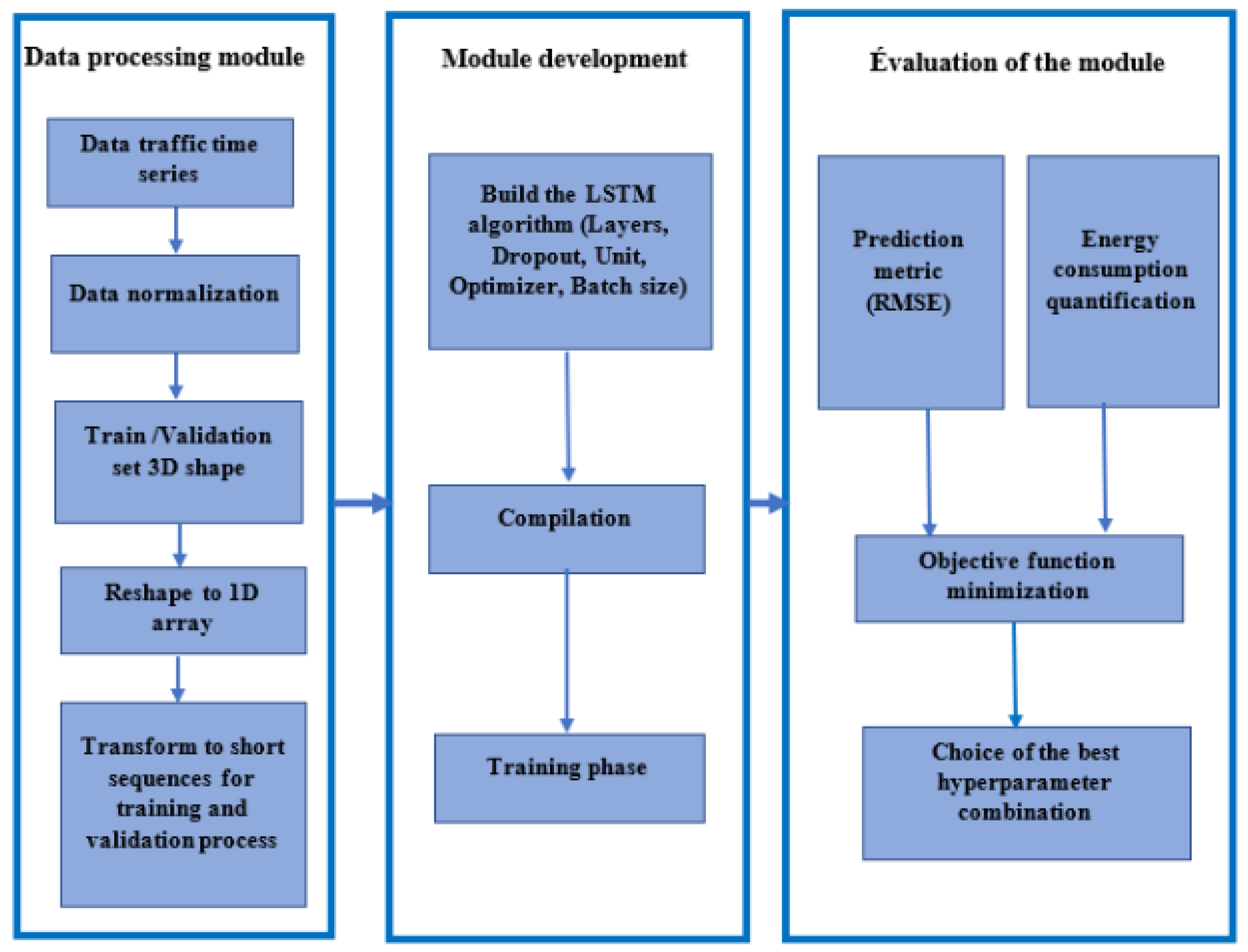
2.1. Data Processing Module

2.1.1. Dataset

The data used in this research were published by Kaggle [27]. The data were collected from 4G cell traffic. The dataset includes 57 cells (BSs) for approximately one year (1 year × 24 h × 57 cells). The database under study then contains the following fields:
  • Cell ID (57 cells).
  • Date and time: timestamp of the traffic measurement.
  • Traffic: cell-specific traffic at each timestamp.

2.1.2. Data Normalization and Transformation

Cellular data are considerably complex and are composed of underlying signals with vastly different properties. Moreover, cell data is distributed randomly. To alleviate the effect of outliers from our analyses, min-max normalization is considered. This technique scales data into the range (0, 1). The formula used to achieve this is as follows [28]:
x n o r m a l i z e d = x m i n   ( x ) m a x   ( x ) m i n   ( x )
where m i n   ( x ) is the minimum of the data and m a x   ( x ) is the maximum value of the data traffic. Real-time prediction of data traffic requires continuous data input and learning. Hence, we employ the notion of the sliding window, which indicates a fixed number of previous timeslots to learn and then predict the current data traffic. Finally, we split the processed data into two sets: training and testing. Our feature set should contain the traffic values for the last 24 h, while the label or dependent variable should be the traffic value at the 25th hour. In order to train the LSTM (Long Short-Term Memory) model by use of a training dataset, data needs to be converted into the shape acceptable for LSTM architecture. Therefore, data require reshaping into a three-dimensional format. The first dimension is the number of records or rows in the dataset, which in this case is 8732. The second dimension is the number of time steps, which is 24, and the last dimension is the number of indicators that are equal to 1 for the given dataset.

2.2. Module Development

There are two parameters used in the proposed module: hyperparameters and model parameters. Hyperparameters are parameters supplied to the model (e.g., model architecture, activation function, and more) and differ from model parameters (e.g., weights and biases) derived from backpropagation training stage. Hyperparameters control the learning; for this reason, we have recently used hyperparameter optimization to accurately predict cellular data through a machine learning algorithm [29].
In this study, we consider approximately all contributing hyperparameters to capture the entire impacts of hyperparameters: the number of layers, the number of neurons per layer, the dropout rate, and the optimizers. To reduce energy consumption and enhance prediction performance simultaneously, the values of these hyperparameters need to be optimized. To this end, we considered the following methods.

2.2.1. Grid Search

The most widely used method to optimize hyperparameter configuration space is the grid search (GS) [30]. GS can be described as an exhaustive exploration search algorithm that evaluates all the combinations of hyperparameters given in the grid configuration. GS operates by assessing the Cartesian product of a finite set of values defined by the user.
In our experiment, the GS was used to generate the error values and energy consumption as a function of the possible combinations of the hyperparameters. This will help to exploit and analyze the effects of the hyperparameters on the performance and energy consumption of the model. First, we defined the range of possible values for the hyperparameters (Table 1). Then, we trained the model for each combination from the predefined list of values. We generated 12,288 combinations corresponding to 12,288 training. The model is then evaluated based on two criteria: energy consumption and model performance using Equation (10), described below. Once all the combinations are evaluated, the model with the hyperparameter set that achieved the best performance and the lowest energy consumption is considered optimal.

2.2.2. Long Short-Term Memory (LSTM)

LSTM is a special kind of Recurrent Neural Network (RNN) with additional features to memorize the sequence of data. They were explicitly designed to avoid long-term dependency issues, which is the cause of the gradient problem in normal RNNs. The ability to learn long-term dependencies is due to the structure of LSTM units, which incorporate gates that regulate the learning process. The structure of the LSTM unit contains forget gate f t , candidate layer C ¯ t , input gate I t , output gate O t , and memory state C t . The relevant mathematical formulas are as follows [31]:
f t = σ X t W f + H t 1 W f + b f
C ¯ t = tanh   ( X t W C ¯ + H t 1 W C ¯ + b C ¯ )
I t = σ X t W i + H t 1 W i + b i
O t = σ X t W o + H t 1 W o
C t = f t C t 1 + I t C ¯ t
H t = O t t a n h C t
where X t is the input vectors, H t 1 is the previous output cells, C t 1 are the previous memory cells, H t are the current output cells, C t are the current memory cells, W, b are the weight matrices, and the bias vectors, respectively. Using the combination of these equations, the LSTM unit can be expressed as follows:
h t = f ( h t 1 , X t , ψ )
where f is the LSTM function and ψ is the vector parameter in the LSTM.
The input gate determines whether or not to let the new input in. An output gate decides what information to output, and memory gate chooses which new data must be stored in the cell. These gates are analog gates based on the sigmoid function, which works in the range 0–1.

2.2.3. The Learning Algorithm

Optimization is carried out by retraining the model with different combinations of hyperparameters (optimizer, batch size, number of layers, number of neurons per layer) and evaluating its performance (energy consumption and prediction accuracy). The training steps of the model are listed in the Algorithm 1.

Optimizers

Optimizers play a crucial role in improving performance and training speed. Selecting an appropriate optimizer is a non-trivial task. The choice of optimizer depends on the specific problem and the tradeoffs between computation time, convergence speed, and accuracy. In our study, we opted for the three most commonly used optimizers in sequential data problems; Adam (Adaptive Moment Estimation), RMSprop (Root Mean Square Propagation), and Nadam (Nesterov-accelerated Adaptive Moment Estimation).
Adam is a first-order gradient-based optimization method for stochastic objective functions based on lower-order adaptive moment estimates. The advantages of using Adam include ease of implementation, efficient computation, and low memory requirements.
RMSprop divides the weight learning rate by a moving average of magnitude. The magnitude sizes of the gradients vary by weight and evolve over time, hence the difficulty of selecting a single global learning rate. This aspect of issue is handled by RMSProp by maintaining a moving average of the squared gradient and changing the updates of the weights by this magnitude.
Nadam is an extension of the Adam algorithm that incorporates the Nesterov momentum and can lead to better performance of the optimization algorithm.

Dropout

The dropout layer was added to improve the predictive performance of the model and prevent overfitting [32]. In the dropout layer, the model randomly deactivates the neurons in a layer with a certain probability. When the dropout value is added to a layer, the neural network will ignore selected neurons during training, and the training time will be faster. In general, the dropout rate can range from 0.1 to 0.5. However, it is important to note that choosing the optimal dropout rate is typically a trial-and-error process, and can depend on factors such as the complexity of the model, the amount of training data, and the task being performed. In our case, we chose rates of 0.1 and 0.2 based on the complexity of the model and our database. We considered various factors to find the best dropout value for our model, including the effects of regularization on learning and the overall performance of the model.

Batch Size

One of the main hyperparameters to adjust before starting the training process is the batch size. The batch size is a parameter that specifies the number of training samples that will be used during training to perform an update of the network parameters [33]. To determine the impact of batch size on model consumption, we set the batch size between 32 and 512 with a step of 32, because our model begins to stabilize from 512.

Hidden Layers

Hidden layers consist of recurrent cells whose states are affected by both past states and current inputs with feedback connections. Recurrent layers can be organized in various architectures to form different LSTMs. Different cells and internal connections, therefore, allow the LSTMs to have different capabilities. To investigate the impact of the hidden layers on the power consumption and performance of the model, we considered their number ranging from 1 to 4, because beyond 5 layers, the model began to exhibit overfitting due to the increased complexity of the network compared to our dataset.

Number of Units Per Layer

The units indicate how many neurons are in a specific layer. We carefully considered the number of neurons per layer for our model architecture, and ultimately decided on values ranging from 8 to 256. Our decision was based on several factors, including the size and complexity of our dataset, as well as the nature of the task at hand. We found that beyond 256 neurons, the model became increasingly complex and prone to overfitting.
Alglgorithm 1: Algorithm of the Proposed Method
1Input: Traffic data
2Output: The minimized objective function
3Data preparation
4Split Data (training set/validation set)
5Defining min-max scaler
6Fitting with min-max scaler
7Reshaping data
8EPOCH: 120
9Create the LSTM network
10  For number layers from 1 to 4 do
11  For Optimizer = [Adam, RMSProp, Nadam] do
12  For the Batch size in the range [32, 512, 32] do
13 For Unite in the range [8, 256, 8] do
14  For dropout in the range [0.1, 0.3, 0.1] do
15  Fit the LSTM network
16  Make predictions with train and Validation datasets
17  Calculate the root mean square error and quantify the energy consumed
18  Calculate the objective function
19  End
20  End
21  End
22  End
23  End
24Choice of hypermeters for which the objective function is minimal

2.3. Evaluation Module

The proposed framework was evaluated using different hardware and software environments. Table 2 shows the equipment used to assess the proposed method.
To evaluate the performance of the proposed model, the Root Mean Square Error (RMSE) was used to estimate the prediction accuracy, and the PyRAPL tool was used within this study to quantify the energy consumption as a function of the hyperparameter combination.
Each time we tested different hyperparameters, the model needed to be trained on the training data, predictions made on the validation data, and the model needed to be evaluated.

2.3.1. Evaluation Metrics with RMSE

We opted for the RMSE metric, which measures the average error between the predicted values and the real values, taking into account the square root of the deviations. This metric is particularly useful for evaluating the performance of regression models with outliers, as it further penalizes large errors. RMSE is a measure often used to evaluate the accuracy of the prediction obtained by the model. The formula for calculating RMSE is as follows:
R M S E = 1 N ( y i y i ^ ) 2
RMSE measures the square root of the mean of the deviation squares, which quantifies the difference between the predicted values and the actual ones. Where y i is the actual value, y i ^ is the predicted value, and N represents the total number of predicted traffic data.

2.3.2. Measurement of Energy Consumption

To measure the impact of hyperparameters on the energy consumption of the model, the energy consumption of the algorithm during its execution needs to be measured. This experiment used PyRAPL, which provides a Python interface to Intel “Running Average Power Limit” (RAPL) technology. RAPL estimates the power consumption of a CPU and has been available on Intel CPUs since the Sandy Bridge generation. RAPL provides measurements for the energy consumption of the whole CPU socket package [34].
All experiments were performed on a PC with an Intel(R) Core (TM) i5-1035G1 processor, running at a speed of 1.00 GHz 1.19 GHz, with 8 GB of RAM, and running on the Windows 10 operating system. The deep learning model was implemented using the Tensorflow 2.4.1 library and the Python programming language. The complete model was trained on a single CPU for 120 epochs, which took approximately 520 h.

2.3.3. Objective Function Minimization

Our problem addresses the tradeoffs involved in a two-objective optimization problem, minimization of energy consumption and prediction error. For this, we defined the objective function ( O F m i n ) as follows:
O F m i n = W 1 2 E c E c , u E c , m a x 2 + W 2 2 R M S E R M S E , u R M S E , m a x 2 1 2
where, E c and RMSE are the energy consumption and the error, respectively. Subscript u refers to the utopia solution, while max refers to the maximum values of the objective functions. The utopia solutions for this problem can be assumed to be equal to zero, where W 1 and W 2 are used as weights to scale and give priority to the terms.

3. Results and Discussion

In this section, the results of the simulation and optimization are presented and discussed.

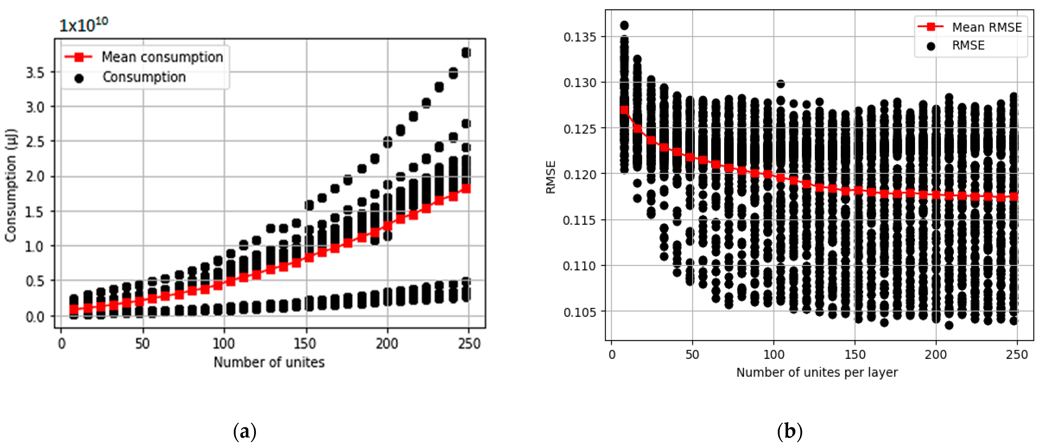
3.1. Exploiting the Influence of the Number of Units per Layer on the Energy Consumption and Performance of the Model

To exploit the influence of the number of units per layer on the energy consumption and performance of the model, we defined the range of units between 8 and 256 with a step of 8 and with a large search space of 7022 hyperparameter combinations. Figure 2a shows the evolution of the energy consumed in microjoules as a function of the number of units per layer. Each point in Figure 2a corresponds to a set of hyperparameters from the ranges defined in Table 1.
Figure 2b presents the dependence of RMSE on the number of neurons per layer. The simulation results show that a large number of units per layer increases the power consumption for training the model. However, the prediction error decreases with the increase in the number of units per layer. There is therefore a tradeoff which should be managed in such a way that energy consumption is minimized, and prediction accuracy simultaneously remains acceptable.
We concluded that the number of units affects the energy consumption and the performance of the model. Thus, if the goal of the problem is to achieve the best performance, then a large number of units is the most appropriate solution. However, if power consumption is the major factor in an application, then a large number of units is unfavorable. In addition, increasing the number of units unnecessarily leads to an overfitting problem.

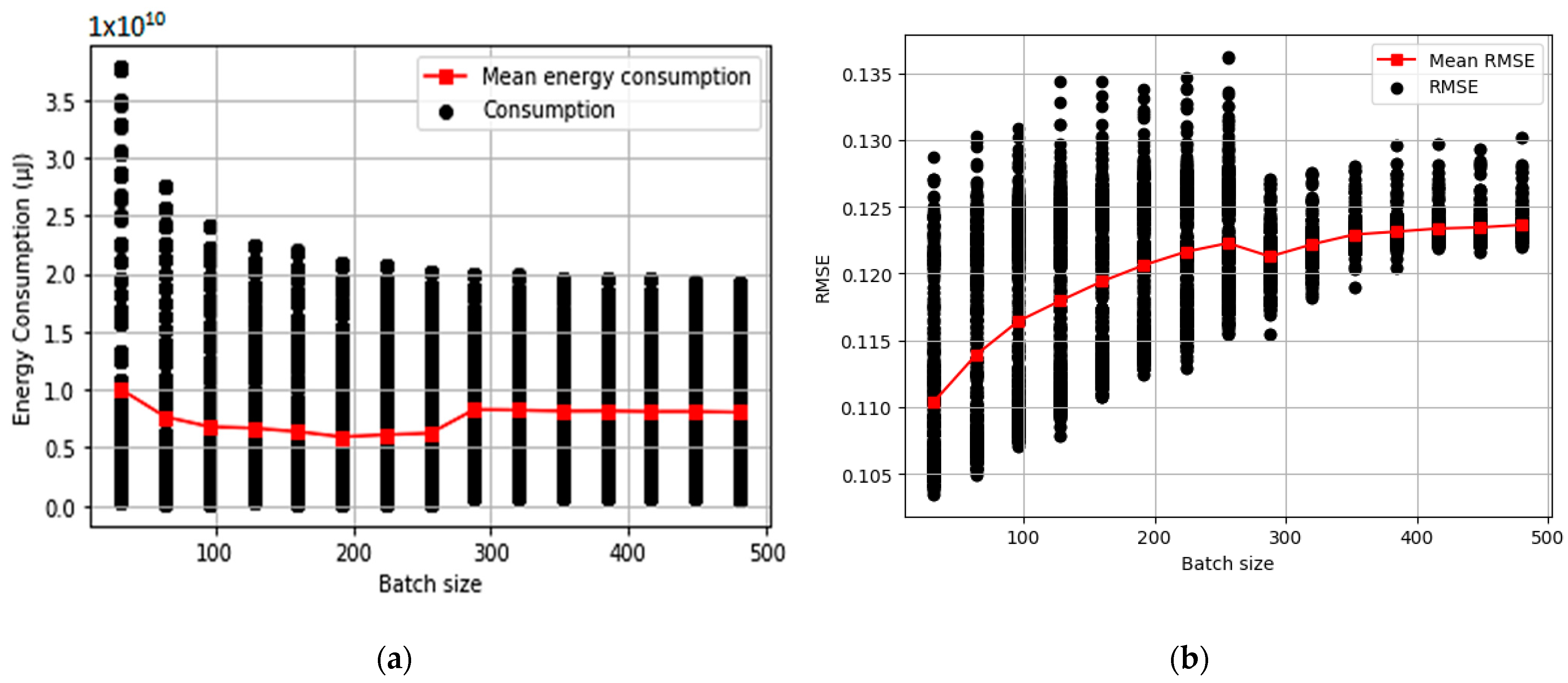
3.2. Exploitation of the Influence of the Batch Size on Energy Consumption and Model Performance

In this section, we assess the impact one of the most important hyperparameters. The goal is to determine the impact of batch size hyperparameter on the energy consumption and accuracy of the proposed deep learning model. To obtain consistent results, different values for the batch size are chosen (Table 1).
Figure 3a,b summarizes the simulation results related to the impact of batch size on energy consumption and performance. We can see in Figure 3a that energy varies with the value of the batch size, and the largest value of the energy consumed by the model is for the small values of the batch size. This is due to small batch sizes require more resources (CPU and software) to see all the data and higher number of iterations. Figure 4b shows the variation of the RMSE as a function of batch size. In Figure 3b, we can see that the batch size of 32 gives raise to the best result, and the large RMSE values resulted in batch size values of less than 250.
It is evident from these simulations that energy consumption increases with the decrease in the batch size, but the performance improves with the increase in the batch size. These results demonstrate that using a large batch size minimizes the energy but increases the prediction error of the model. From these results, we can conclude that the batch size has a significant impact on the energy consumption and performance of the model. Thus, a large batch size should be used to reduce energy consumption and achieve good model performance.

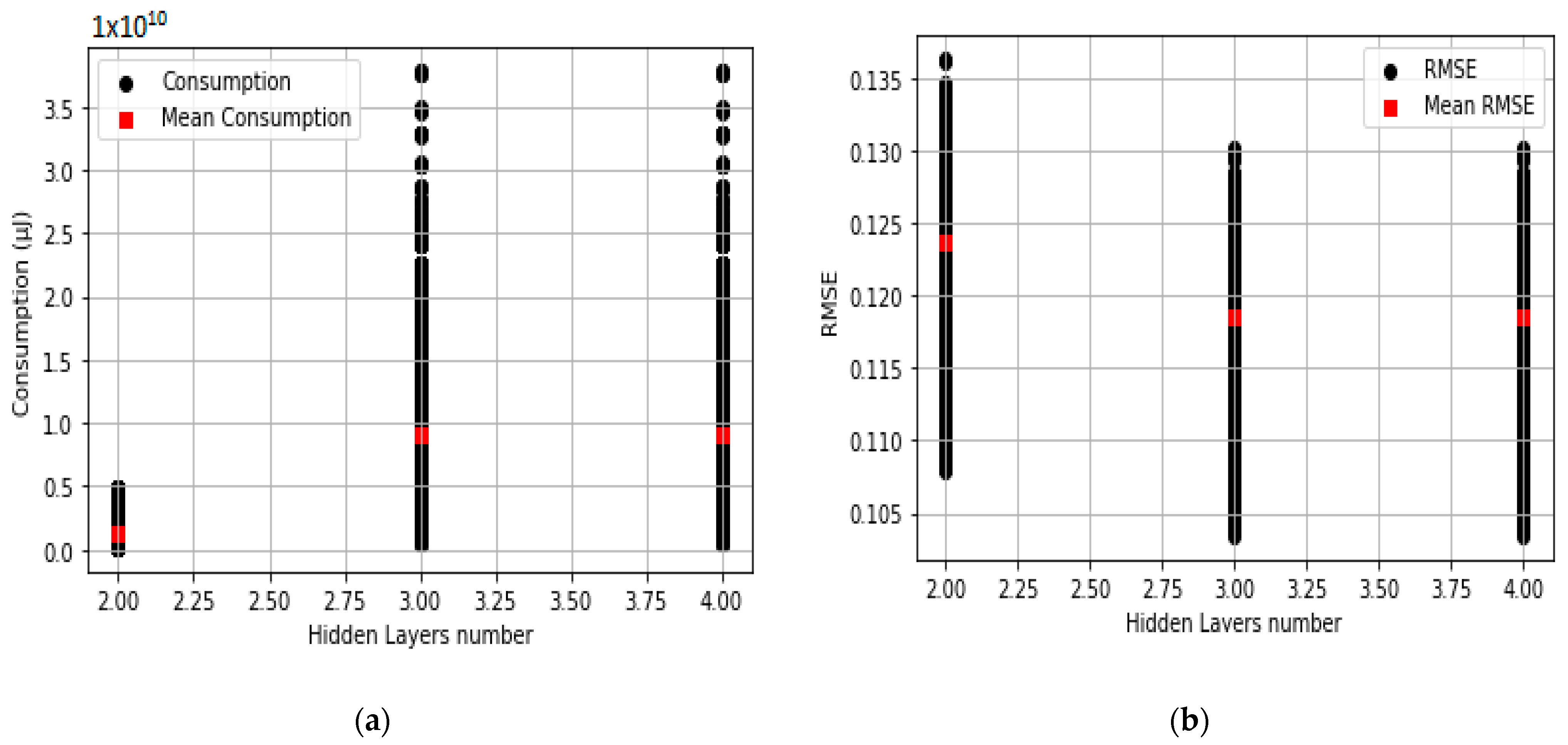
3.3. Impact of the Number of Layers on the Energy Consumption and Performance

In order to study the influence of the hidden layers on the energy consumption and performance of our model, we changed the values of the hidden layers from two to four. Figure 4a shows the energy consumption of the model as a function of the number of hidden layers. We can see that the energy consumption is lowest with two layers. However, there is no difference between the energy consumption of three and four layers.
To analyze the influence of the number of hidden layers on the prediction accuracy, the variation of RMSE as a function of the number of hidden layers is shown. Based on the simulation results shown in Figure 4b, it can be seen that the prediction error is low when the number of layers is three or four. However, the RMSE is high when the number of layers is two.
Selecting the number of hidden layers in a neural network is one of the major problems in the field of artificial neural networks. Arbitrary selection of the number of hidden layers can lead to high power consumption and lower model accuracy. If power consumption is the most important criterion in an application, a small number of hidden layers is more suitable, but if the performance of the model is the most important factor, a large number of hidden layers is more suitable.

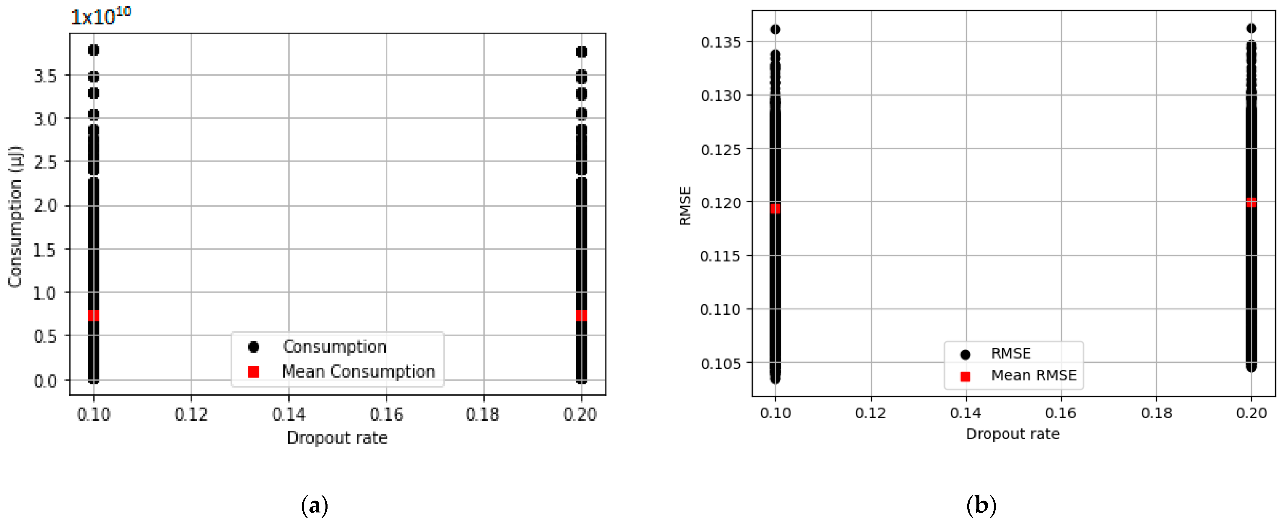
3.4. Exploiting the Impact of Dropout Rate on Energy Consumption and Model Performance

The regularization of neural networks is an important task for the reduction of overfitting. Dropout is a widely used regularization approach for neural networks.
In this section, we analyze the impact of the dropout rate on model energy consumption and performance. For this purpose, we tested different values for the dropout rate, shown in Table 1. Figure 5a,b shows the evolution of the model’s energy consumption and prediction error, respectively, as a function of the dropout rate. From Figure 5a,b, it can be seen that the dropout rate has no effect on energy consumption and prediction error.
Based on these observations, we conclude that the dropout rate has no effect on the model energy consumption and performance. However, dropout is more widely used to prevent overfitting.

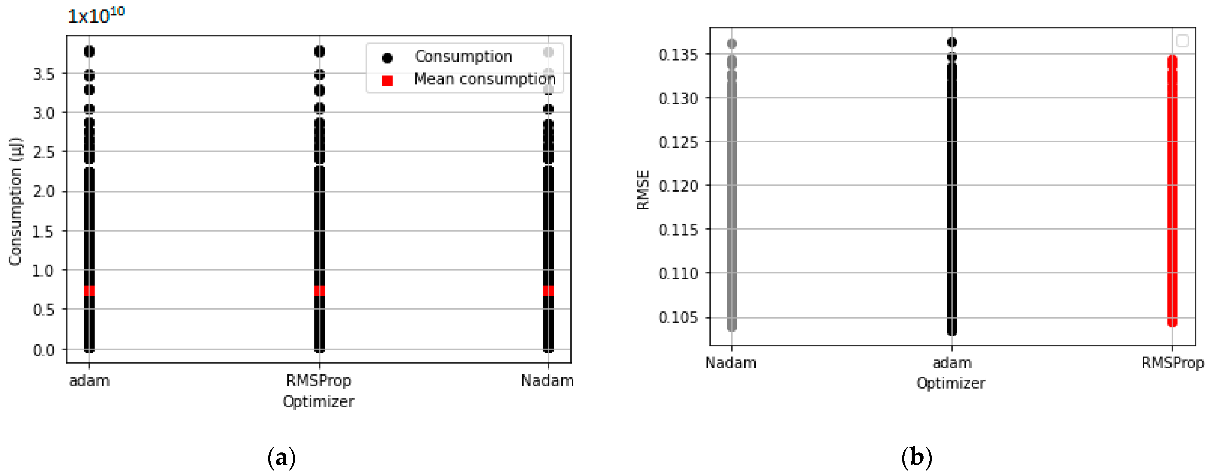
3.5. Examining the Influence of Optimizer Type on Energy Consumption and Model Performance

The optimizer is an important hyperparameter for neural network tuning, but it has not received much attention. To illustrate the impact of optimizer type on the energy consumption and performance of our model, we selected three optimizers that are most commonly used in prediction problems: Adam, RMSprop, and Nadam.
Figure 6a, b demonstrates the impact of optimizer type on energy consumption and error prediction, respectively. For this, we tested three types of optimizers: Adam, Nadam, and RMSprop.
From the data shown in Figure 6a, b, we can see that there is no difference in energy consumption between the different optimizers, but in terms of model performance, RMSprop shows superior performance. Adam and RMSprop provide the same performance.
The selection of an optimization algorithm for the training process has a significant influence on the performance results. From the experiment results, we conclude that the type of optimizer does not affect the energy consumption of the model, but the type of optimization influences the performance of the model.

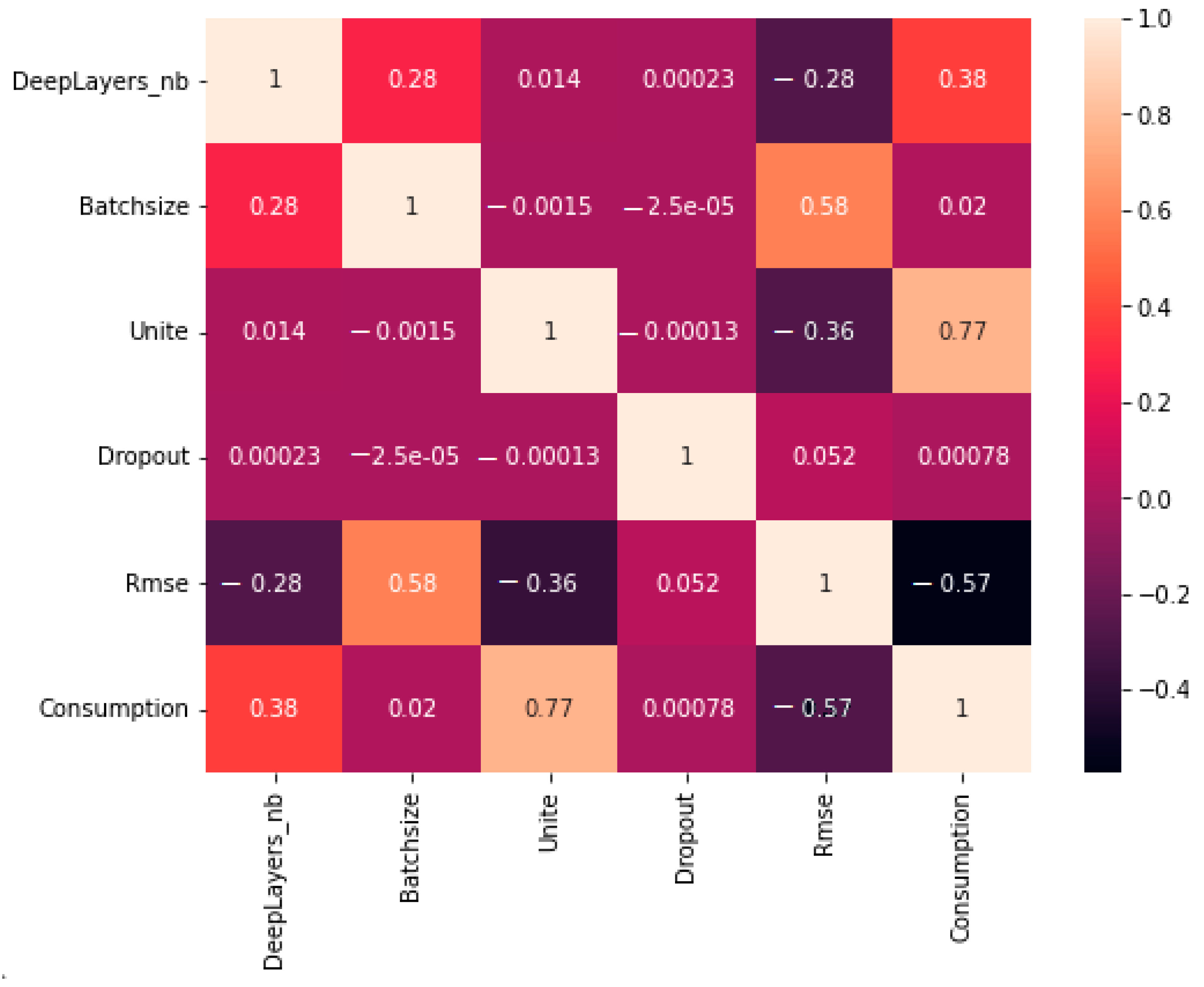
3.6. Correlation Matrix

To assess the interdependence between the hyperparameters, energy consumption, and the performance of the model, we chose the widely-used Pearson correlation. This statistical technique produces a correlation coefficient that ranges from −1 to +1, representing the strength and direction of a linear relationship between two variables. A correlation coefficient of +1 implies a perfect positive correlation, where an increase in one variable is associated with a proportional increase in the other variable. In contrast, a correlation coefficient of −1 indicates a perfect negative correlation, where an increase in one variable corresponds to a proportional decrease in the other variable. When the correlation coefficient is 0, there is no linear relationship between the two variables. A correlation coefficient greater than 0.7 is deemed a strong correlation, implying a robust linear relationship, whereas a correlation coefficient less than 0.3 is considered a weak correlation, indicating a less pronounced linear relationship.
Next, we focused on identifying the best combination of hyperparameters that would allow for low energy consumption and superior performance. Figure 7 shows the correlation matrix used to study the dependency between the different hyperparameters, energy consumption, and model prediction error, simultaneously.
In the correlation matrix, the Pearson correlation coefficients between the hyperparameters, energy consumption, and RMSE are indicated. It can be observed that there is a very strong correlation of 0.77 between the number of units and the energy consumption of the model, which means that an increase in the number of units per layer increases the energy consumption. Additionally, there is a moderate dependence of 0.38 between the number of hidden layers and the energy consumption of the model, implying that increasing the number of layers moderately increases the energy. It can also be observed that there is a weak correlation between the dropout rate and energy, indicating that an increase in dropout rate does not affect the energy consumed by the model.
A relatively strong correlation of 0.58 is observed between the batch size and the prediction error, meaning that an increase in batch size will increase the error. The correlation between RMSE and the number of units per layer is −0.38, so an increase in the number of layers will reduce the prediction error. It can also be observed that there is a moderate negative correlation of −0.28 between RMSE and the number of hidden layers, indicating that increasing the number of hidden layers moderately reduces the error. Regarding the dropout rate and RMSE, there is a weak correlation between the two parameters, so the dropout rate does not affect the prediction error.

3.7. The Best Hyperparameters

In order to determine the optimal hyperparameters for our model, we utilized Equation (10) and examined two main criteria: minimizing energy consumption and ensuring acceptable prediction error. By varying the weight values, we were able to identify the ideal combination of hyperparameters that yielded the lowest objective function, as shown in Table 2.
From our analysis, we found that assigning equal weight values of 0.5 to w1 and w2 leads to the best combination of hyperparameters to reach the minimum objective function. This combination included three hidden layers, a batch size of 64, 184 units, the use of an RMSprop optimizer, and a dropout rate of 0.1.
However, we also recognized the importance of prioritizing specific criteria depending on the goals of the model. To emphasis on minimizing energy consumption, we adjusted the weight values to w1 = 0.3 and w2 = 0.7, which led to the optimal combination of hyperparameters consisting of three hidden layers, a batch size of 64, 184 units, the use of a Nadam optimizer, and a dropout rate of 0.1.
Conversely, to prioritize reducing the error in the objective function, we chose w1 = 0.7 and w2 = 0.3, which resulted in a different optimal combination of hyperparameters: three hidden layers, a batch size of 32, 72 units, the use of a Nadam optimizer, and a dropout rate of 0.1.
Overall, our approach demonstrates the importance of carefully considering the relative weights of different criteria when optimizing the hyperparameters, in order to achieve the desired outcomes for the model.

4. Related Work

Past research has inadequately explored the effects of hyperparameters on the model performance and energy consumption. Table 3 compares our study with other relevant publications. We have particularly emphasized the importance of energy efficiency in machine learning and proposed different approaches to optimize energy consumption, while maintaining a reasonable level of accuracy. Different datasets, machine learning algorithms, and techniques were used in those studies. However, in our work, we showed for the first time, to the best of our knowledge, a novel approach to analyze and optimize hyperparameters in a deep learning algorithm during the training phase, aiming to achieve a better balance between algorithm performance and energy consumption. This proposed framework could be expanded to other cellular networks (e.g., 5G) and energy optimization approaches.

5. Conclusions

In this study, a bottom-up framework was developed and implemented to consider the impact of hyperparameters on model performance and energy consumption. The study highlights the importance of selecting an appropriate set of hyperparameters to optimize model performance and minimize energy consumption of deep learning algorithms used in cellular traffic prediction. Moreover, the study used a multi-objective optimization approach to simultaneously minimize the Root Mean Square Error (RMSE) and energy consumption, resulting in an optimal tradeoff solution. We have shown that an appropriate set of hyperparameters contributes significantly to improved model performance and energy consumption. The proposed method presented in this paper paves the way to investigate the impact of hyperparameters on energy consumption and error prediction in deep learning models.

Author Contributions

Conceptualization, S.T. and F.B.; methodology, S.T. and F.B; software, S.T.; validation. and, F.B.; formal analysis, S.T.; investigation, L.T.; data curation, S.T.; writing—original draft preparation, S.T.; writing—review and editing, F.B and L.T.; visualization, F.B.; supervision, L.T and F.B. All authors have read and agreed to the published version of the manuscript.

Funding

This research received no external funding.

Institutional Review Board Statement

Not applicable.

Informed Consent Statement

Not applicable.

Data Availability Statement

Not applicable.

Acknowledgments

The authors are grateful to Sayyed Ahmad Khadem for useful discussions and comments on the manuscript.

Conflicts of Interest

The authors declare no conflict of interest.

References

  1. Hill, K. Connected Devices will be 3x the Global Population by 2023, Cisco Says. RCR Wireless News, 18 February 2020. Available online: https://www.rcrwireless.com/20200218/internet-of-things/connected-devices-will-be-3x-the-global-population-by-2023-cisco-says(accessed on 26 October 2022).
  2. 5G and Its Impact on the Internet of Things—Stardust Testing. Available online: https://www2.stardust-testing.com/en/5g-and-impact-on-iots (accessed on 26 October 2022).
  3. You, X.; Zhang, C.; Tan, X.; Jin, S.; Wu, H. AI for 5G: Research directions and paradigms. Sci. China Inf. 2019, 62, 21301. [Google Scholar] [CrossRef]
  4. Wu, J.; Zhang, Y.; Zukerman, M.; Yung, E.K. Energy-efficient base-stations sleep-mode techniques in green cellular networks: A survey. IEEE Commun. Surv. Tutor. 2015, 17, 803–826. [Google Scholar] [CrossRef]
  5. Richter, F.; Fettweis, G.; Gruber, M.; Blume, O. Micro base stations in load constrained cellular mobile radio networks. In Proceedings of the IEEE 21st International Symposium on Personal, Indoor and Mobile Radio Communications Workshops, Istanbul, Turkey, 17 December 2010; pp. 357–362. [Google Scholar]
  6. Shu, Y.; Yu, M.; Liu, J.; Yang, O.W.W. Wireless traffic modeling and prediction using seasonal ARIMA models. IEICE Trans. Commun. 2005, 88, 3992–3999. [Google Scholar] [CrossRef]
  7. Zhang, D.; Liu, L.; Xie, C.; Yang, B.; Liu, Q. Citywide cellular traffic prediction based on a hybrid spatiotemporal network. Algorithms 2020, 13, 20. [Google Scholar] [CrossRef]
  8. Liang, D.; Zhang, J.; Jiang, S.; Zhang, X.; Wu, J.; Sun, Q. Mobile traffic prediction based on densely connected CNN for cellular networks in highway scenarios. In Proceedings of the IEEE 11th International Conference on Wireless Communications and Signal Processing, Xi’an, China, 23–25 October 2019; pp. 1–5. [Google Scholar]
  9. Zhang, C.; Zhang, H.; Yuan, D.; Zhang, M. Citywide cellular traffic prediction based on densely connected convolutional neural networks. IEEE Commun. Lett. 2018, 22, 1656–1659. [Google Scholar] [CrossRef]
  10. Chen, R.; Liang, C.; Hong, W.; Gu, D. Forecasting holiday daily tourist flow based on seasonal support vector regression with adaptive genetic algorithm. Appl. Soft Comput. 2015, 26, 435–443. [Google Scholar] [CrossRef]
  11. Jnr, M.D.; Gadze, J.D.; Anipa, D. Short-term traffic volume prediction in UMTS networks using the Kalman filter algorithm. Int. J. Mob. Netw. Commun. Telemat. 2013, 3, 31–40. [Google Scholar]
  12. Nie, L.; Jiang, D.; Yu, S.; Song, H. Network traffic prediction based on deep belief network in wireless mesh backbone networks. In Proceedings of the IEEE Wireless Communications and Networking Conference (WCNC), San Francisco, CA, USA, 19–22 March 2017; pp. 1–5. [Google Scholar]
  13. Qiu, C.; Zhang, Y.; Feng, Z.; Zhang, P.; Cui, S. Spatio-temporal wireless traffic prediction with recurrent neural network. IEEE Wirel. Commun. Lett. 2018, 7, 554–557. [Google Scholar] [CrossRef]
  14. Global Emissions. Center for Climate and Energy Solutions. 24 March 2022. Available online: https://www.c2es.org/content/international-emissions/ (accessed on 26 October 2022).
  15. IEA. Digitalization and Energy-Analysis, IEA. Available online: https://www.iea.org/reports/digitalisation-and-energy (accessed on 26 October 2022).
  16. García-Martín, E.; Rodrigues, C.F.; Riley, G.; Grahn, H. Estimation of energy consumption in machine learning. J. Parallel Distrib. Comput. 2019, 134, 75–88. [Google Scholar] [CrossRef]
  17. Lacoste, A.; Luccioni, A.; Schmidt, V.; Dandres, T. Quantifying the carbon emissions of machine learning. arXiv 2019, arXiv:1910.09700. [Google Scholar]
  18. Strubell, E.; Ganesh, A.; Mccallum, A. Energy and policy considerations for deep learning in NLP. arXiv 2019, arXiv:1906.02243. [Google Scholar]
  19. Anthony, L.F.; Wolff, K.B.; Selvan, R. Carbontracker: Tracking and predicting the carbon footprint of training deep learning models. arXiv 2020, arXiv:2007.03051. [Google Scholar]
  20. Stamoulis, D.; Cai, E.; Juan, D.; Juan, D.; Marculescu, D. Hyperpower: Power-and memory-constrained hyper-parameter optimization for neural networks. In Proceedings of the 2018 Design, Automation & Test in Europe Conference & Exhibition (DATE), Dresden, Germany, 19–23 March 2018; pp. 19–24. [Google Scholar]
  21. Canziani, A.; Paszke, A.; Culurciello, E. An analysis of deep neural network models for practical applications. arXiv 2016, arXiv:1605.07678. [Google Scholar]
  22. Rodrigues, C.F.; Riley, G.; Luján, M. SyNERGY: An energy measurement and prediction framework for Convolutional Neural Networks on Jetson TX1. In Proceedings of the International Conference on Parallel and Distributed Processing Techniques and Applications (PDPTA), Las Vegas, NV, USA, 13–16 July 1998; The Steering Committee of The World Congress in Computer Science, Computer Engineering and Applied Computing (WorldComp): Las Vegas, NV, USA, 2018; pp. 375–382. [Google Scholar]
  23. Yang, T.-J.; Chen, Y.; Sze, V. Designing energy-efficient convolutional neural networks using energy-aware pruning. In Proceedings of the IEEE Conference on Computer Vision and Pattern Recognition, Honolulu, HI, USA, 21–26 July 2017; pp. 5687–5695. [Google Scholar]
  24. Brownlee, A.E.; Adair, J.; Haraldsson, S. Exploring the accuracy—Energy trade-off in machine learning. In Proceedings of the 2021 IEEE/ACM International Workshop on Genetic Improvement (GI), Madrid, Spain, 30 May 2021; pp. 11–18. [Google Scholar]
  25. Dai, X.; Zhang, P.; Wu, B.; Yin, H.; Sun, F.; Wang, Y. Chamnet: Towards efficient network design through platform-aware model adaptation. In Proceedings of the IEEE/CVF Conference on Computer Vision and Pattern Recognition, Long Beach, CA, USA, 15–20 June 2019; pp. 11398–11407. [Google Scholar]
  26. Brownlee, A.E.I.; Burles, N.; Swan, J. Search-based energy optimization of some ubiquitous algorithms. IEEE Trans. Emerg. Top. Comput. Intell. 2017, 1, 188–201. [Google Scholar] [CrossRef]
  27. Alsaade, F.W.; Hmoud Al-Adhaileh, M. Cellular traffic prediction based on an intelligent model. Mob. Inf. Syst. 2021, 2021, 6050627. [Google Scholar] [CrossRef]
  28. Borkin, D.; Némethová, A.; Michaľčonok, G. Impact of data normalization on classification model accuracy. Res. Pap. Fac. Mater. Sci. Technol. Slovak Univ. Technol. 2019, 27, 79–84. [Google Scholar] [CrossRef]
  29. Khadem, S.A.; Bensebaa, F.; Pelletier, N. Optimized feed-forward neural networks to address CO2-equivalent emissions data gaps—Application to emissions prediction for unit processes of fuel life cycle inventories for Canadian provinces. J. Clean. Prod. 2022, 332, 130053. [Google Scholar] [CrossRef]
  30. Belete, D.M.; Huchaiah, M.D. Grid search in hyperparameter optimization of machine learning models for prediction of HIV/AIDS test results. Int. J. Comput. Appl. 2022, 44, 875–886. [Google Scholar] [CrossRef]
  31. Arulampalam, G.; Bouzerdoum, A. A generalized feedforward neural network architecture for classification and regression. Neural Netw. 2003, 16, 561–568. [Google Scholar] [CrossRef] [PubMed]
  32. Srivastava, N.; Hinton, G.; Krizhevsky, A.; Sutskever, I.; Salakhutdinov, R. Dropout: A simple way to prevent neural networks from overfitting. J. Mach. Learn. Res. 2014, 15, 1929–1958. [Google Scholar]
  33. Brownlee, J. Difference between a Batch and an Epoch in a Neural Network, Machine Learning Mastery. 15 August 2022. Available online: https://machinelearningmastery.com/difference-between-a-batch-and-anepoch (accessed on 26 October 2022).
  34. Pyrapl, PyPI. Available online: https://pypi.org/project/pyRAPL/ (accessed on 26 October 2022).
Figure 1. Schematic representation of the proposed framework and methodology.
Telecom 04 00013 g001
Figure 2. (a) Variation of energy consumption as a function of the number of units per layer. (b) Variation of RMSE as a function of the number of units per layer.
Telecom 04 00013 g002
Figure 3. (a) Variation of energy consumption as a function of the batch size. (b) Variation of RMSE as a function of the batch size.
Telecom 04 00013 g003
Figure 4. (a) Variation of energy consumption as a function of the hidden layer number. (b) Variation of RMSE as a function of the hidden layer number.
Telecom 04 00013 g004
Figure 5. (a) Variation of energy consumption as a function of the dropout rate. (b) Variation of RMSE as a function of the dropout rate.
Telecom 04 00013 g005
Figure 6. (a) Variation of energy consumption as a function of the type of the optimizer. (b) Variation of RMSE in function as a function optimizer.
Telecom 04 00013 g006
Figure 7. Correlation matrix used to identify key trends.
Telecom 04 00013 g007
Table 1. Hyperparameters values.
HyperparametersValues
Optimizer[Adam, RMSProp, Nadam]
Batch size[32–512 with a step of 32]
Layers number[1, 2, 3, 4]
Number of Neurons in each layer[8–256 with step of 8]
Dropout rate[0.1, 0.2]
Epoch120
Activation functionReLu
Table 2. Optimization result.
WeightsLayersBatch SizeNumber of UnitsOptimizerDropout O F m i n
W1 = W2 = 0.5364184RMSprop0.10.39397401
W1 = 0.7
W2 = 0.3
364184Nadam0.10.24012428
W1 = 0.3
W2 = 0.7
33272Nadam0.10.54496929
Table 3. Comparison with related work.
ReferencesMachine Learning AlgorithmsDatasetApproaches
[24]Multilayer perceptronMedical data set (diabetes, glass, ionosphere, iris) Explored the tradeoff between energy consumption and accuracy for different hyperparameter configurations of a popular machine learning framework
[25]Neural network ImageNetThis approach leverages existing efficient network building blocks and focuses on exploiting hardware characteristics and adapting computational resources to accommodate target latency and/or power constraints.
[20]Neural NetworksNot statedHyperPower, a framework that enables efficient Bayesian optimization and random search in the context of power- and memory-constrained
[26]Multilayer perceptronNot statedTool for measuring the energy consumption of JVM programs using a bytecode level model of energy cost.
[16]Convolutional neural network
Data stream mining
Poker-Hand
Forest
Cover type
The goal is to provide useful guidelines to the machine learning community, giving them the fundamental knowledge to use and build specific energy estimation methods for machine learning algorithms.
Proposed workRecurrent neural network (LSTM)Traffic data setExploring and optimizing the hyperparameters of machine learning algorithms employed in cellular traffic prediction.
Disclaimer/Publisher’s Note: The statements, opinions and data contained in all publications are solely those of the individual author(s) and contributor(s) and not of MDPI and/or the editor(s). MDPI and/or the editor(s) disclaim responsibility for any injury to people or property resulting from any ideas, methods, instructions or products referred to in the content.

