Article

Aspen Plus® Modeling and Simulation of an Industrial Biomass Direct Liquefaction Process

by
Duarte M. Cecílio
1,2,*,
J. Ricardo M. Gonçalves
1,2,
Maria Joana Neiva Correia
2 and
Maria Margarida Mateus
1,2
1
Secil S.A., Fábrica Secil—Outão, 2901-864 Setúbal, Portugal
2
CERENA—Centro de Recursos Naturais e Ambiente, Departamento de Engenharia Química, Instituto Superior Técnico, Universidade de Lisboa, 1049-001 Lisboa, Portugal
*
Author to whom correspondence should be addressed.
Fuels 2023, 4(2), 221-242; https://doi.org/10.3390/fuels4020014
Submission received: 19 February 2023 / Revised: 26 April 2023 / Accepted: 17 May 2023 / Published: 26 May 2023

Abstract

:
The current energy and climate crisis calls for immediate action in replacing fossil fuels with those derived from renewable sources. The Energreen process performs the direct liquefaction of biomass to produce a liquid biofuel for the cement industry and an aqueous solution of added-value compounds for further processing. The present work details the development of an Aspen Plus® model to simulate this biomass liquefaction process. The proposed model describes the Energreen liquefaction process using simplified reaction kinetics and thermodynamic models. The model was validated using data from a real liquefaction pilot plant with a deviation of 6.4%. The simulation, conducted with several biomass samples of variable compositions, showed that the process is robust enough to deal with different compositions and, due to the substitution of the fossil fuels presently used in the cement plant, it will allow savings of up to USD 102,000 per year to be achieved. Several analyses of the sensitivity of the results to the process variables were performed and it was possible to identify the reactor temperature and the reaction activation energy as the most impactful parameters on the process output. Overall, the results allow us to conclude that the proposed model is a solid framework for the optimization of industrial liquefaction processes.

1. Introduction

The depletion of fossil-based resources and the environmental impact of their consumption has accelerated the drive for replacing non-renewable fossil fuels with more sustainable alternatives such as biomass. Biomass can be used directly as fuel or it can be processed to produce new fuels and to recover a wide variety of chemical compounds, some of which present a significant added value in various chemical industries. The processing or upgrading of biomass can take place through biochemical and thermochemical processes.
The former focuses on the enzymatic hydrolysis of biomass, while the latter is divided into the three processes gasification, pyrolysis, and liquefaction, the last of which is the subject of this work [1]. Liquefaction can be carried out in different conditions at high temperatures (>200 °C) and pressures, as in hydrothermal upgrading (HTU), or at moderate temperatures (100–250 °C) and atmospheric pressure in the presence of a solvent and a catalyst, as in direct liquefaction [2]. Previous studies have shown that the yield of liquefaction is affected by several factors, such as the type of biomass feedstock, the solvent, the type and concentration of the catalyst, and the reaction time [2].
Despite the relatively mild processing conditions, which simplify the reactor design, the varying feedstock composition can result in different product compositions. Therefore, the biomass feedstock is a crucial system boundary condition to consider, and understanding the different reaction pathways in an intricate network of possibilities is essential in modeling the liquefaction process [3].
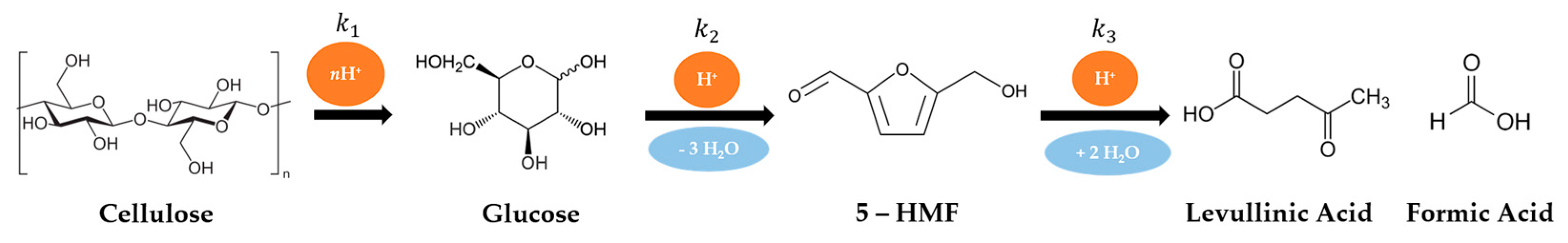
This work focuses on processing lignocellulosic biomass, which is mainly formed by three biopolymers: cellulose (40–60 wt.%), hemicellulose (20–40 wt.%), and lignin (10–25 wt.%). Cellulose is a linear polymer made up of repeating glucose units bonded by β-1,4-glycosidic bonds, which make it resistant to chemical attack [4]. As any polymer, cellulose can be crystalline or amorphous, and crystalline cellulose is not depolymerizable at low temperatures, as the diffusion of the solvent and catalyst inside the polymer structure is hindered.
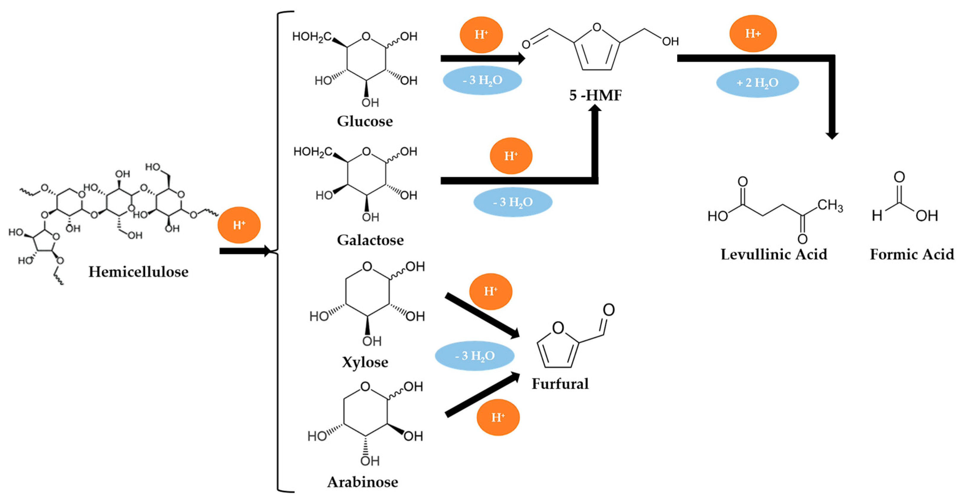
Hemicellulose is an amorphous heteropolymer formed by linear chains of pentoses and hexoses: xylose and arabinose as C5 sugars, and galactose, glucose, or mannose as C6 sugars. The polymer chains are usually branched with other sugars, carboxylic acids, and sometimes phenolic compounds. Due to its chemical composition and linear structure, hemicellulose is easily hydrolysable under mild conditions [4].
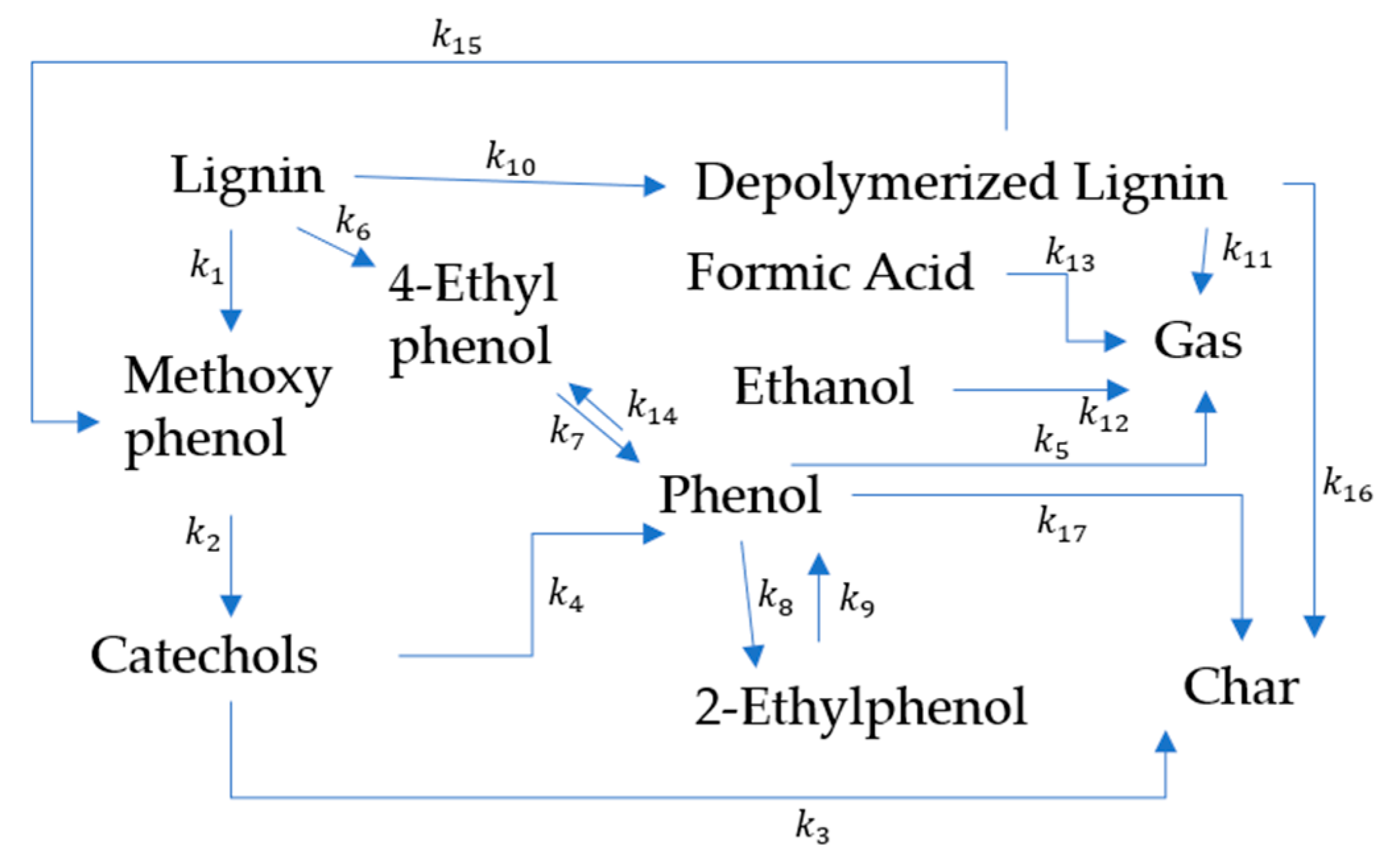
Contrary to cellulose and hemicellulose, lignin is a highly branched amorphous biopolymer, mainly composed of phenolic alcohols such as p-coumaryl, synapil, and conyferil alcohols. This high degree of branching leads to a three-dimensional network, which is difficult to chemically depolymerize [4].
There are several mathematical and computational models proposed in the literature to describe the liquefaction process, mostly for hydrothermal liquefaction (HTL), which intend to provide a better understanding of the reactions network and allow mass and energy balances to be performed for the production process, to estimate, for example, the product yields. Braz et al. [1] performed a series of experiments designed to study the effect of the catalyst concentration and temperature on pine wood sawdust thermochemical liquefaction. These experiments were used to adjust a simple kinetic model for reaction yield prediction. Hao et al. [5] describe in their work advances regarding the use of empirical models, response surface methods, kinetic models, and machine learning models for the optimization of biomass hydrothermal liquefaction. The authors highlight the capabilities of kinetic modeling and machine learning in predicting and optimizing biomass HTL processes subject to a wide range of feedstock compositions. Other authors [6,7] developed models to predict not only yields but also bio-oil and biocrude properties. Using a multiphysics approach, Ranganathan et al. [8] modeled the hydrothermal liquefaction of microalgae in a plug-flow reactor using the computational fluid dynamics software COMSOL Multiphysics 5.3. The authors presented a model that can adequately predict reactor temperature profiles, HTL product yields for the process, and that can be used as a tool for reactor scale-up and design. Ou et al. [9] used the ChemCAD 6.5 software for chemical process modeling and economic cost estimation to evaluate the technical and economic feasibility of producing transportation fuel by HTL of defatted microalgae and subsequent hydroprocessing of the biocrude. The authors concluded that the minimum selling price of the fuels obtained from the process are economically competitive with those of conventional fuels. Several studies were also published based on the Aspen Plus® software suite for chemical process modeling and simulation. For example, Hoffman et al. [10] used Aspen Plus® V7.3 to model and simulate a conceptual process combining an HTL plant with a biogas plant. The proposed process produces biogas, biocrude, and upgraded biofuels that can be used directly for transportation or for combined heat and power production. The necessary mass balances and the technical and economic feasibility of the proposed process are also presented. Pedersen et al. [11] developed a model using Aspen Plus® (unspecified version) to demonstrate the technical and economic feasibility of a conceptual process to produce drop-in fuels through HTL. The authors found that the proposed process is highly competitive when compared with other production alternatives and concluded that HTL optimization is the key factor to increase the competitiveness of the overall process. Ong et al. [12] used Aspen Plus® to obtain the mass and heat balances of a patented 2000 t/day HTL plant, processing pine wood Kraft black liquor to yield a gasoline/diesel blend. The authors reached a minimum fuel selling price slightly higher than that of gasoline in the United States and concluded that heat and exergy recovery are key factors to reach an economically competitive process.
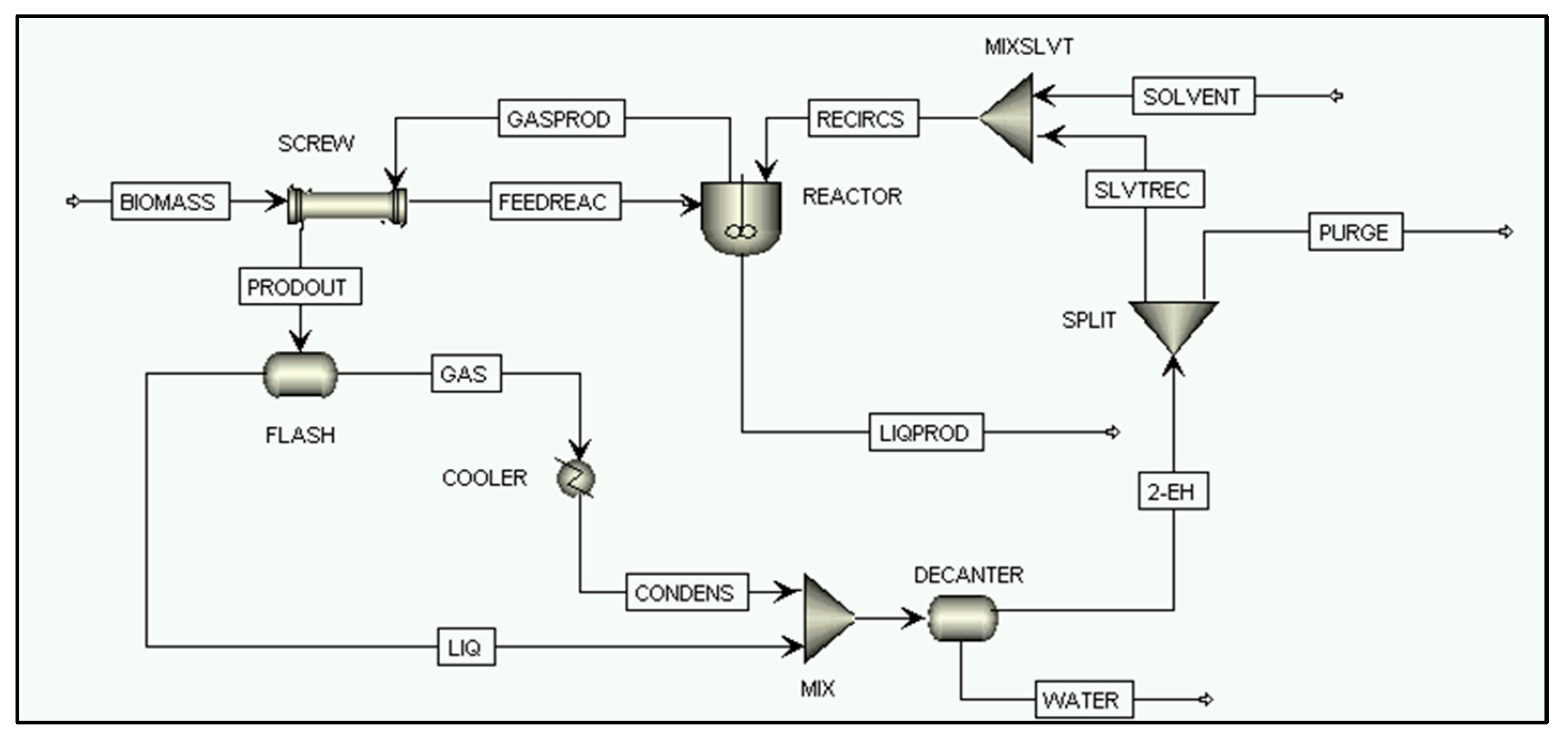
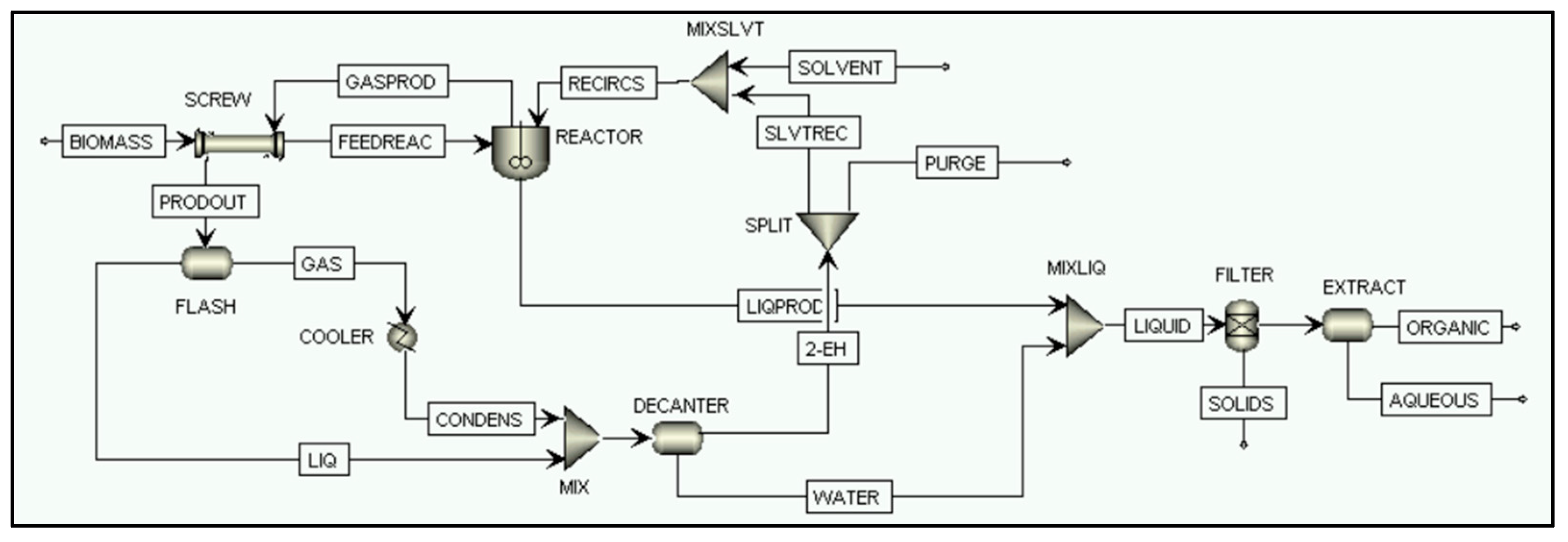
As mentioned above, direct liquefaction uses significantly milder conditions (<200 °C, 1 atm) than HTL, which constitutes an a priori advantage to achieve economic feasibility. Nevertheless, to the authors’ knowledge, there are no models published in the literature for the direct liquefaction of biomass. Therefore, this work intends to present the establishment of a model to describe the acid-catalyzed direct liquefaction of wood biomass to produce a biofuel for direct use in heavy duty kilns and added-value chemicals in a biorefinery perspective.

2. Liquefaction Process and Model Implementation

2.1. The Energreen Liquefaction Process

The Energreen project was initially developed with the aim of producing a sustainable biofuel (bio-oil) through acid liquefaction of lignocellulosic feedstocks. The produced biofuel can have an important role in helping the industrial transition from fossil to greener fuels. In fact, due to its low oxygen content (10–11%), the Energreen fuel should have a high performance as a fuel and, when compared to conventional diesel, it will allow a CO2 emissions reduction higher than 75% [13].
It is known that biomass liquefaction is a significantly complex process due to the large variety of physico-chemical reactions that occur simultaneously. Several of these chemical reactions compete with each other and their occurrence is strongly influenced by the operating conditions (temperature, biomass type and composition, solvent, catalyst, etc.). From these, the temperature is one of the most important variables to consider, as a low reaction temperature will lead to low liquefaction yields but high temperatures can lead to repolymerization reactions [14,15]. Likewise, biomass composition is also an important variable, and its lignin content is the most critical factor. In fact, the complex three-dimensional structure results in a lower depolymerization yield compared to the cellulose and hemicellulose moieties. The latter components do not significantly affect the reaction yield due to their simpler structures [15,16]. However, as mentioned before, cellulose crystallinity is an important characteristic, as the tight molecular organization in the crystalline domains of polymers presents a strong stereochemical hindrance that severely slows down the reaction kinetics compared to the amorphous domains. Finally, the solvent type also influences the liquefaction yield due to the different solvolysis mechanisms that can take place [1,12]. Hydrogen donor solvents typically present higher conversion rates and better biofuel quality by simultaneously promoting hydrodeoxygenation reactions and inhibiting repolymerization [17].
The present work is based on the patented Energreen process [18,19]. This project involved the assembly and start-up of a semi-industrial pilot plant in the CMP held facility at Pataias, Portugal, which is represented in Figure 1. In this process, biomass goes through a swelling treatment that facilitates the access of the catalyst to the biomass polymers. The reaction occurs at temperatures between 130–180 °C with mechanical stirring. The solvent is added to the reactor in a range of 0–50% compared to the biomass feed rate, whereas the catalyst used was p-toluenosulfonic acid, added in a loading percentage between 0.01–3 wt.% of the biomass amount [18,19]. This solid organic acid is easier to process than sulfuric or hydrochloric acids, which are also corrosive and consequently demand stricter safety measures [1].
In short, the Energreen process can be described as a sequence with the following steps: biomass pretreatment, liquefaction, and filtration. In the pretreatment step the biomass contacts with the solvent in the screw conveyor to promote its swelling and is preheated to avoid quenching the reaction medium. Afterwards, the pretreated biomass enters the reactor and, after the desired residence time, the reaction mixture is removed from the reactor and filtered to separate the unreacted solids from the bio-oil. In the following sections, the different stages of the process will be detailed.

2.1.1. Biomass and Catalyst Feeding

The biomass used in the process, which can have a wide range of compositions regarding the lignocellulosic compounds, is fed through hopper 1 (4 in Figure 1), which can deal with materials of up to 30 mm in size. The catalyst p-toluenosulfonic acid is added through hopper 2 (5 in Figure 1).

2.1.2. Pretreatment

The raw material and catalyst are both dosed through a rotary valve. The resulting mixture is then fed to the screw conveyor, where an amount of solvent is injected to promote the swelling of the biomass which improves the catalyst’s access to the biopolymers. This endless screw is one of the most important pieces of equipment of the whole system since it allows the biomass to be transported to the reactor and to carry out simultaneously the biomass swelling and the mixture preheating by contact counter-currently with the vapor phase released from the reactor. Additionally, as mentioned above, a certain amount of solvent or of the produced bio-oil is sprayed onto the biomass to promote its swelling. In fact, the lignocellulosic material absorbs the atomized liquid leading to an increase in the cells’ volume, which facilitates the catalyst’s access to the polymeric chains, thus promoting their breakdown. A solvent tank and a series of injectors are needed to inject the solvent through a common rail mechanism.

2.1.3. Liquefaction

The liquefaction reaction takes place in a 316 L stainless steel reactor which is resistant to the corrosion that can take place as a result of the use of an acid medium. A torisperhical head sits on top of the vessel and the bottom is double crowned and self-cleaning. The design of the reactor vessel bottom results from the need to avoid the accumulation of unreacted solid matter during the reaction. Furthermore, the reaction mixture is continuously stirred, to ensure homogeneity, by a helicoidal stirrer.
It is known that lignocellulosic biomass liquefaction is an endothermic process and, as such, the reactor is equipped with a thermal oil heating coil. To improve the thermal efficiency of the process, the reactor is also equipped with an external heating jacket where the boiler hot flue gases can circulate.
The reaction is carried out at atmospheric pressure, which means that the reactor is equipped with pressure release valves that are activated accordingly to avoid pressure buildup. The steam used to preheat the reaction mixture inside the screw conveyor results from the evaporation of the biomass moisture during the reaction. Depending on the steam flowrate, a condenser is needed on the opposite end of the screw conveyor to fully condense the vapors that failed to condense by contact with the biomass. The cooling fluid of the condenser is industrial water, with a maximum flowrate of 5 m3/h.

2.1.4. Filtration

The reaction mixture is removed through the bottom of the reactor by means of a mushroom valve. When the valve is open, the mixture passes through a self-cleaning basket filter to remove the solid particles. This filter is crucial not only to separate the solid material from the liquefied biomass, but also to provide information on the extent of the reaction through quantification of the solid matter that has not reacted. This residual solid is recirculated to the reactor and the liquid phase is injected into the screw conveyor to promote the biomass swelling with no additional solvent use. When the liquefaction process achieves the desired yield, the biofuel is then pumped to 1 m3 containers for further physical and chemical characterization, namely its heating value.

2.2. Aspen Plus® Model Implementation

Due to the lack of available data, modeling, and simulation of the described liquefaction processes in Aspen Plus® V11.1 required some approximations to be made. First, the catalyst molecule was not included in the model but its effect was taken into account through the kinetic rate constants from the literature. Additionally, the swelling system was also not simulated and the small amount of solvent used for swelling was introduced directly in the reactor with the remaining solvent. The recirculation of the non-reacted solid to the reactor was likewise not considered in a preliminary stage. It should be mentioned that the process described in the preceding sections is a batch process, whereas the following model intends to simulate continuous operation, which can yield significant cost and energy savings.

2.2.1. Chemical Compound Setup

The simulated biomass liquefaction process is a catalytically aided process that takes place at 160 °C in a continuously stirred tank reactor (CSTR). The catalyst used in the process is p-toluenosulfonic acid and 2-ethylhexanol (2-EH) is used as solvent. As previously mentioned, in this simulation the contribution of the catalyst was taken into account through the kinetic rate constants chosen for each reaction.
The introduction of cellulose, hemicellulose, and lignin in the simulation also required some simplifications. In fact, only cellulose is present in the Aspen Plus® database and was added as is. Conversely, hemicellulose and lignin were added separately as their respective monomers: xylose, galactose, glucose, and arabinose represent the hemicellulose moiety and p-coumaryl alcohol was added to represent the lignin component [3,7,20]. Additionally, the intermediate and final products of the hydrolysis were also added. These were water, glucose, 5-hydroxymethylfurfural (HMF), levulinic acid, formic acid, furfural, and phenol (Table 1). The chemical reactions are explained in greater detail in the following sections. The introduction of the above mentioned relevant chemical compounds required the following Aspen Plus® V 11 databases: APV110 ASPENPCD, APV110 AQUEOUS, APV110 SOLIDS, APV110 INORGANIC, APV110 PURE37, NISTV110 NIST-TRC, APV110 POLYMER.
Furthermore, the thermodynamic method chosen to predict the thermodynamic and transport properties of the compounds was NRTL-RK. This model is recommended for chemical compounds with more than five carbon atoms [21].

2.2.2. Missing Physical and Thermodynamic Properties

Some of the added compounds required additional properties or parameters which were missing in the software database and were complemented with data from the literature. Cellulose required the input of its standard enthalpy of formation (DHFORM), which was found to be 963 kJ/mol [22]. P-coumaryl alcohol required the introduction of several parameters to calculate its vapor pressure, molar heat capacity, and vaporization enthalpy, which were obtained in the work published by Gorensek et al. [23]. According to Gorensek et al. [23], the vapor pressure (in pascals) was calculated through the extended Antoine equation:
ln p = 2,867,075 25,124.63 T 37.26739 ln T + 1.48627 × 10 5 T 2 ; 406.15 T 791.4
with the temperature in K and pressure in pascals. These values must be introduced in Aspen Plus® in the PLXANT-1 parameter responsible for the calculation of the component’s vapor pressure.
The heat capacity of p-coumaryl alcohol was calculated using the following Aly–Lee equation. The relevant parameters were introduced in Aspen Plus® using the CPALE-1 parameter.
c p = 128,972.6 + 342,667.4 1575.222 T sinh 1575.222 T 2 + 266,861.9 728.2816 T sinh 728.2816 T 2 ; 298 T 1000
where the temperature is in K and the heat capacity in J/kmol.K−1. Finally, the vaporization enthalpy was calculated using the Watson equation, introducing the relevant coefficients in parameter DHVLWT.
H v a p T = H v a p T 1 1 T T C 1 T 1 T C a + b 1 T T C ; T > T m i n
From this calculation, the value for the enthalpy of vaporization at 25 °C is 59.7 kJ/mol. Parameters a and b were assumed to take the default values, which are 0.38 and 0, respectively. A value of 273 K was also assumed for Tmin.

2.2.3. Feedstock Characterization

In the simulated process, the biomass and solvent are both directly fed to the reactor. Thus, 62 kg/h of biomass, with a moisture content of 16.7% according to the pilot plant data, was fed to the reactor. As such, the complete biomass feed flowrate comprised 74 kg/h of wet biomass at 25 °C and atmospheric pressure. The biomass ash content was initially disregarded in the simulation, and an average composition of 50% cellulose, 30% hemicellulose, and 20% lignin in the biomass feedstock was assumed [4]. As previously stated, hemicellulose was represented by glucose, xylose, arabinose, and galactose, with all components considered to exist in equal proportions. The operational conditions and composition of the feed stream can be seen in Table 2 and Table 3.
The solvent inlet stream was fed at 25 °C and atmospheric pressure and its flowrate was calculated from the process mass balances. In the experimental run of the pilot plant, 2600 kg of biomass was added for 42 h, along with 1956 kg of solvent, which corresponds to a biomass flowrate of 62 kg/h and a solvent flowrate of 47 kg/h. This led to the creation of a design spec in Aspen Plus®, which maintains the desired solvent feed flowrate independently from the remaining parameters.
With the recirculation of the solvent to the reactor, a purge stream is necessary to avoid the accumulation of compounds inside the reactor vessel. An initial value of 0.1 for the purge fraction was used.

2.2.4. Direct Biomass Liquefaction Process Simulation

With all of the necessary compounds and properties defined, the process was simulated in Aspen Plus®. The process flowsheet is depicted in Figure 2.
The process feed streams depicted in the flowsheet are named BIOMASS and SOLVENT. The former carries the biomass to the endless screw conveyor, wherein a preheating takes place by indirect contact with the vapor exiting the reaction. The latter transports the solvent make-up to the reactor. As outputs of the system, the streams PURGE, ORGANIC, and AQUEOUS are represented.
The screw conveyor (SCREW) that feeds the biomass into the reactor is represented by a concentrical tube heat exchanger, which heats up the biomass to a temperature of 90 °C before entering the reactor. The hot stream of this heat exchanger is the stream GASPROD, made up of the 2-EH, water, and some residual volatile liquefaction products.
At one end of the SCREW, the preheated biomass enters the reactor, whereas at the other end, the stream GASPROD is converted into the stream PRODOUT, which is admitted into a flash separator to separate its liquid and vapor fractions. It is worth noting that this flash separator is not a representation of a piece of equipment from the actual process but rather a mathematical tool to accurately simulate the differences between the vapor and liquid fraction of the stream, which are a direct result of the vapor–liquid equilibrium inside the screw. After separation, the gaseous part of the stream is condensed in the condenser (COOLER), after which it is mixed (block MIX) with the flash liquid stream. Afterwards, a decanter (DECANTER) is introduced to separate the components of the water/solvent mixture.
The organic phase obtained from the decanter, rich in 2-EH, is then recirculated to the reactor to decrease the solvent make-up. However, as the recirculated solvent contains a residual fraction of liquefaction products, a purge stream is required to avoid product accumulation, which could lead to a severe decrease in the reaction yield and potential stoppages. On the other hand, the aqueous phase separated from the mixture is combined with the liquefied product coming out of the reactor, which allows for a liquid–liquid extraction to take place in a second decanter (EXTRACT) to obtain the ORGANIC and AQUEOUS streams. Before the EXTRACT there is a FILTER, where 95% of the solids (non-liquefied biomass—cellulose, glucose, galactose, p-coumaryl alcohol, xylose, and arabinose) are removed from the stream.

SCREW

The SCREW block is simulated as a HeatX heat exchanger. This equipment is a concentrical tube indirect counter-current heat exchanger where the biomass moves in the center tube and the reaction vapors removed from the reactor move along the outer tube. The primary specification of the SCREW block is that it heats up the biomass from 25 °C to 90 °C.

REACTOR

The preheated biomass is fed to the REACTOR block, along with the make-up solvent. In the reactor, the liquefaction reactions take place at atmospheric pressure and a temperature of 160 °C, in a useful volume of 9.78 m3; the liquid phase presents an average residence time of 2 h. The reactor model chosen was the RCSTR and the modeled liquefaction reactions are described in the following sections.

Biomass Liquefaction Reactions

As previously mentioned, biomass is composed of cellulose, hemicellulose, and lignin in certain proportions, which depend on the type of biomass (hardwood, softwood, herbaceous, etc.). Cellulose hydrolysis results in glucose, which in turn decomposes into 5-HMF. This compound is unstable in an acid medium and decomposes into levulinic acid and formic acid, which are more stable at low pH. Therefore, these two compounds are considered to be the final products (Figure 3).
The kinetic parameters of cellulose hydrolysis were studied by Yan et al. [24]. The kinetic profiles were assumed to be irreversible reactions of pseudo-first order and the relevant constants, shown in Table 4, were obtained from [24]. The data used to reach theses value are provided in the Supplementary Material (Tables S1–S3).
k = k 0 exp E a R T
As stated above, in this simulation hemicellulose is described by glucose, xylose, arabinose, and galactose. Thus, glucose and galactose directly decompose to 5-HMF, that subsequently reacts with water yielding levulinic acid and formic acid, whereas xylose and arabinose yield furfural. These reactions are depicted in Figure 4.
The decomposition of hemicellulose was assumed to be described by pseudo-first order kinetics. The Arrhenius equation parameters (Table 5) were obtained for the hemicellulose biopolymer and not for its monomers. However, the kinetic parameters of the monomers were considered to be the same as those of hemicellulose [26].
Lignin decomposition reactions (Figure 5) are mechanistically more complex when compared to cellulose and hemicellulose (Figure 4) and yield several phenolic-based compounds. Therefore, a simplified representation of lignin was considered using p-coumaryl alcohol to yield phenol. Once again, a pseudo-first order kinetic law was assumed, and the relevant parameters can be consulted in Table 5.

FLASH

The FLASH block is responsible for separating the phases of the product stream that exits the screw. As previously mentioned, this flash separator is conceptual, as in reality the screw has a different outlet for the liquid and vapor streams. The FLASH separator works at atmospheric pressure and is considered to work adiabatically.

COOLER

The COOLER equipment is designed to completely condense the vapor stream that exits the previous FLASH block. As such, block specifications include atmospheric pressure and no vapor fraction at the outlet stream.

MIX, MIXSLVT, MIXLIQ

The MIX, MIXSLVT, and MIXLIQ blocks are all mixers that mix different streams at atmospheric pressure. The MIX block combines the material streams LIQ and CONDENS to feed them to a decanter. MIXSLVT is responsible for combining the recirculation stream with the solvent make-up before admission to the reactor. Finally, MIXLIQ adds the aqueous phase of the decanter to the liquid product stream exiting the reactor performing a liquid–liquid extraction.

DECANTER

The DECANTER separates the two phases of the 2-EH and water mixture. The former will be recirculated to the reactor, while the latter is used for hydrophilic compound extraction. The decanter works at atmospheric pressure and a temperature of 25 °C.

SPLIT

The SPLIT block is a separator that represents the purge of the recirculated solvent stream. The purge fraction chosen was 10%.

FILTER

The FILTER is the equipment where the solid fraction of the outlet reactor stream is separated. The FILTER removes 95% of the solid particles in the inlet stream as a result of the performance of the filter installed in the real plant. The components that are filtered out are those used to describe the solids.

EXTRACT

The EXTRACT block is also a decanter to carry out the liquid–liquid extraction to separate the hydrophilic compounds of the bio-oil from the hydrophobic ones. The decanter works at atmospheric pressure and 25 °C.

3. Simulation Results

3.1. Results

3.1.1. Model Validation

Model validation was performed by comparing its output with the results of an experimental liquefaction run conducted in the pilot plant of Pataias using a Eucalyptus biomass with the composition described in Table 6.
Table 7 describes the experimental run conditions and results obtained in the pilot plant.
As previously mentioned, it is important to consider that the experimental run was conducted in a semi-continuous operation mode, where the biomass, solvent, and catalyst quantities were fed in increments, as well as the product recovered, which was removed from the reactor in increments. The reaction was conducted for a total duration of 3 days. This reaction time was used to convert the data into continuous operation to compare with the model results. Due to the scarce amount of characterization data available, the validation was performed by essentially comparing the amount of liquefied product obtained from the run and the model, neglecting the 2-EH solvent that is also removed with the product. Table 8 summarizes the results.
The validation results presented in Table 8 show a 6.4% deviation between the model and the experimental run results. This slight underestimation of the product yield can be justified by a combination of factors. Firstly, the model considers pure continuous operation, typical in industrial processes, whereas the pilot plant operates in a semi-continuous mode, which yields batches of product with an average conversion different from a purely continuous reactor. In fact, continuous reactors usually present a bypass effect that can lead to a lower overall yield. Additionally, the experimental pilot reactor has a low-efficiency filter to remove the solid particles from the outlet stream. Since these solid particles correspond to the biomass ash plus the unreacted biomass, the particles that are not retained in the filter will lead to the overestimation of the experimental product yield.
These factors, combined with the simplified kinetics assumed for the different reactions, explain the observed deviation. However, since the deviation is relatively small (below 10%), we can conclude that the model describes quite well the liquefaction process of Eucalyptus biomass. It is also important to consider that the simplifications made to the compounds chosen to represent not only the biomass components but also their subsequent degradation products, can also significantly affect the simulated yield. In fact, the lighter compounds may be more strongly affected by the vapor–liquid equilibria thermodynamics of the modeled system. The lighter compounds volatilize more easily and, thus, are not considered to be present in the liquid phase where the chemical reactions take place.

3.1.2. Fossil Fuel Substitution Simulation

One of the most important applications of this direct liquefaction process is the production of a liquid and easy-to-handle biofuel that can partially or fully be a substitute for the fossil fuels used in different industries, such as the cement industry. The process layout is depicted in Figure 6.
It is worth mentioning that the biofuel produced can also be a source of various value-added compounds from a biorefinery perspective. After the aqueous extraction of these compounds, a new biofuel can be produced, which, due to the extraction of the lighter compounds soluble in water, should have a higher heating value. This approach is depicted in the layout presented in Figure 7 that illustrates an alternative operating mode to produce added-value components that would help to decrease the costs associated with the overall process.
This section focuses on the main objective of the process, which is biofuel production. To that effect, the robustness and versatility of the process is analyzed by simulating the liquefaction of three distinct biomasses, each with its own composition (Table 9).
Reaction conversion and process yield were analyzed for each biomass sample and the values are presented in Table 10, Table 11 and Table 12, whereas the results derived from the simulation are presented in the Supplementary Material (Tables S4–S6).
The calculation of biomass conversion and product yield in the simulation is based on the assumption that the biomass is composed of cellulose, p-coumaryl alcohol, glucose, galactose, arabinose, and xylose. Consequently, the liquefied product is composed of HMF, formic acid, levulinic acid, furfural, and phenol.
Table 10 shows that the reactions of arabinose, cellulose, p-coumaryl alcohol, galactose, and xylose present the same conversion, due to the use of the same kinetic laws that control the reaction extension and of the same operating conditions. As such, the operating pressure and temperature of the reaction, combined with the residence time of the biomass in the reactor, will regulate the final conversion. As the conversion of the reaction is unchanged between biomass samples, a higher cellulose fraction in the feed stream will cause an increase in the amount of unreacted biomass and, consequently, the conversion decreases. This phenomenon is mostly visible for cellulose, as it is the most abundant component.
Table 13 presents the effect of the biomass to solvent mass ratio in the reactor on the product streams’ mass flowrates. As seen, samples 1 and 3, with higher lignin contents, produce a larger flowrate of the gaseous stream. This can be explained by the fact that the decomposition of lignin, represented by p-coumaryl alcohol, yields phenol, which is very volatile, and augments the flowrate of the vapor stream exiting the reactor, which in turn increases the flowrate of the recirculation stream (QINSOLVENT). It is worth noting that this constitutes a limitation of this model that must be further improved to account for lignin-decomposition-derived compounds more accurately, namely in the liquid stream exiting the reactor.
The results of the simulation were then used to predict potential savings in fossil fuels consumption in the cement industry, which is still an important consumer of fossil fuels such as petroleum coke. Therefore, the lower heating value (LHV) of the liquefied biomass was calculated according to Equation (5).
L H V = % s o l v e n t × L H V s o l v e n t + % c a t a l y s t × L H V c a t a l y s t + % d r y   b i o m a s s × L H V d r y   b i o m a s s
As mentioned before, in the current model, the catalyst, which is added in a low quantity, is not considered and, as such, its effect on the LHV is also neglected. On the other hand, the LHV considered for the solvent is 37.6 GJ/t [28], and for Eucalyptus biomass an average value of 18.6 GJ/t [29] was considered. The solvent quantity in the product was taken from the simulation, and Table 14 summarizes the results.
The results show that the LHV of the liquefied product is approximately 24 GJ/t, which is close to the value of 26.9 GJ/t obtained for the real sample produced in the plant, which helps to validate the model. Taking the product yield and its LHV, it is possible to determine the thermal energy substitution. For that, petroleum coke, with an LHV of 31.3 GJ/t [30] and market price of USD 245 per tonne [31] was considered as the fossil fuel to replace, and the results are presented in Table 15.
With the current values, liquefying biomass to produce biofuel can lead to savings of USD 91,000 to 102,000 per year. As future work, a more detailed analysis could be performed considering the power consumption of the plant, utility costs, and the CO2 savings resulting from the fuel substitution.

3.2. Sensitivity Analysis

A model sensitivity analysis was performed to assess the parameters that most strongly affect the product yield, reaction conversion, or any other output variables. The parameters tested were the reactor temperature, purge fraction, biomass moisture content, biomass/solvent ratio, and the reaction activation energy. The results of this sensitivity analysis are presented in the following sections.

3.2.1. Temperature

The results regarding the effect of the reaction temperature on the mass flowrate, reaction conversion, and product yield of several streams are presented in Table 16 and Table 17. The results are shown in the Supplementary Material (Table S7 and Table S8, respectively). It is important to emphasize that the current direct liquefaction process uses temperatures lower than 200 °C, 160 °C in this case, which are significantly lower than the typical temperatures of the most common alternative biomass upgrading processes.
As seen in Table 16, temperature has a strong influence on the flowrates of several streams. Considering the stream LIQPROD, which carries the liquefied product out of the liquefaction reactor, it is possible to observe an inversely proportional relationship with a deviation of 10% in the temperature, resulting in a negative 30% deviation in the liquefied product stream flowrate. This effect may be explained by the vapor–liquid equilibria phenomena taking place in the reactor system. In fact, due to the relatively low difference between the operating temperature (160 °C) and the solvent boiling point (185 °C), particular care must be taken with the control of the process operating temperature to avoid the evaporation of the solvent.
Additionally, due to the kinetic rate laws considered to model the liquefaction reactions, the sensitivity of the conversion of several components to variation in the temperature was also studied (Table 17).
The results of the temperature sensitivity analysis on component conversion show an important landscape that complements the results of Table 16. Despite the higher product stream flowrates (Table 16), a negative variation in temperature of 10/20% results in an overall 25/42% decrease in the process yield and 22/37% in biomass conversion. These results are intimately connected with the kinetic laws since the reaction rate depends exponentially on the temperature. Conversely, for positive increments of the temperature, an increase in the yield and overall conversion is observed. In fact, a 10/20% increase in the temperature leads to a 20/32% increase in the yield, which is a smaller effect than that of decreasing this variable. Furthermore, due to the vapor–liquid equilibria, the favorable effect of the temperature increase can be negated by the choice of solvent and a further increase in the reactor temperature demands the use of a new solvent with a higher boiling point.
It is also important to consider that the simplified kinetic model used in this simulation does not include the kinetic laws for the reverse reactions. Moreover, it is well known that higher temperatures also promote repolymerization reactions. Further refinement of the kinetic model is also important for modeling purposes to further optimize the reactor operating conditions.
The heat duty of COOLER also changes because of the increase in the flow of the GASPROD stream. These changes are reflected in Table 18 (results are shown in Table S9—Supplementary Material).
As expected, the cooler duty has the same tendency as the GASPROD flow. With the increase in flow, the heat needed to condensate all the vapor after the FLASH also increases.

3.2.2. Purge Fraction

The current section details the sensitivity analysis of the model to varying the purge fraction, that is, the fraction of stream 2-EH that is rejected before being reintroduced into the reactor (stream RECIRCS). Recirculation of the solvent stream is a crucial step in reducing solvent waste and ensuring optimal operation of the plant. However, a purge of the stream is necessary to avoid the accumulation of reaction components inside the reaction medium, which can lead to a premature stoppage. Table 19 summarizes the results (Table S10—Supplementary Material) regarding the output variation in the stream flowrate.
The results show that the purge fraction has a moderate effect on the material stream flowrates, with the most affected being the RECIRCS and GASPROD streams, which are, respectively, the recirculated solvent stream and the stream of the vapor product that exits the reactor. The former is a direct result of the purge fraction, and the latter is influenced by the total amount present in the reactor.
The sensitivity of the reaction conversion to the purge fraction was also analyzed. It was observed that the purge fraction has no influence whatsoever in component conversion (Table S11—Supplementary Material). However, this is only true with the current simplified kinetic model. With a more complex model considering reverse reactions, the purge fraction is expected to affect the concentration of the components more strongly in the reaction medium, which in turn should help in displacing the chemical equilibrium, favoring the formation of products rather than reactants.
The purge fraction changes the flow of GASPROD, changing the cooler duty. The deviation is shown in Table 20 and the results in Table S12—Supplementary Material. Due to the dependence that the flow of GASPROD has on the cooler duty, the deviation of both is very similar.

3.2.3. Biomass Moisture Content

Another aspect analyzed in the sensitivity analysis was the biomass moisture content. The initial biomass contains 16.7% moisture, which was used as base for positive and negative deviations of 10% and 20%. The biomass moisture content is expected to influence the vapor–liquid equilibrium phenomena taking place in the reaction medium. The results are presented in Table 21. This table was made based in Table S13—Supplementary Material.
The results show that the variation in the moisture content does not significantly influence the flowrate of the reactor system streams. The deviations observed in the GASPROD stream are moderate, as most of the water leaves the reactor in this stream. In the streams that are directly related to the reactor, the gaseous and liquid outlet streams show slight deviations, which are obtained as a result of the change in the vapor–liquid equilibrium. The larger deviations observed are found in the AQUEOUS stream, which are obtained after liquid–liquid extraction with the evaporated water, as is expected. The biomass moisture does not change the conversion because the operation conditions are the same and—up to a point—are the limiting factor (Table S14—Supplementary Material).
Additionally, the heat duty of the cooler that deals with the vapor product of the reaction suffers change, reflected in Table 22. The results are shown in Table S15—Supplementary Material.
The results shown in the table reflect the expected changes in the vapor–liquid equilibrium while maintaining the operating conditions. That is, the increase in water flow in the GASPROD stream increases the heat duty required for the cooler. The effect of moisture in the conversion of the reactions is null due to the assumed kinetic laws.

3.2.4. Biomass/Solvent Fraction

Another parameter that is known to strongly affect the performance of the process is related to the proportion of the biomass feedstock relative to the amount of solvent introduced to assist the reaction. The stipulated process ratio is 1.33. Consequently, deviations were imposed by altering the amount of solvent introduced in the reactor and the resulting outputs were analyzed. The results are shown in Table 23. This table was based on data in Table S16—Supplementary Material.
The results show that the solvent ratio does not strongly affect the reactor outlet streams or the final streams. This corroborates that in the current model, the main effect of the solvent quantity is the vapor–liquid equilibrium. This behavior is slightly different from that observed when the biomass moisture content is varied, as 2-ethylhexanol is less volatile than water. On the other hand, the decrease in the biomass/solvent ratio presents a positive impact in the mass flow of the organic streams produced in the aqueous extraction of added-value compounds. In fact, it is expected that the shift in the amount of solvent affects the liquid–liquid extraction phenomena and, thus, decreases the mass flowrate of the final AQUEOUS stream. The changes in conversion and overall yield are not significant (Table S17—Supplementary Material).
On the other hand, as shown in (Table 24 and Table S18—Supplementary Material), the cooler heat duty is also affected by the biomass/solvent ratio, also due to changes in the vapor–liquid equilibrium.
Finally, solvent flowrate will increase with the biomass/solvent ratio and so the GASPROD flowrate also increases. This means that the decrease in the biomass/solvent ratio results in a decrease in the heat duty demand in the cooler. On the other hand, there are almost no changes in the reaction conversion with the biomass/solvent ratio.

3.2.5. Activation Energy

The results of the sensitivity analysis to the variation in the activation energy of each reaction, which reflects the effect of the catalyst, on the conversion of every reaction are shown in Table 25 (simulation results presented in Tables S19 and S20 of the Supplementary Material).
The results show a strong correlation between the Ea of each reaction and the flow of the streams. A negative variation in Ea is equivalent to selecting a new catalyst to facilitate the reactions. Thus, for a constant reaction time, a negative variation in the combined activation energies results in an increase in the conversion of each reactant. Likewise, the products of the reactions indicate that the reaction mixture contains higher fractions of volatile components, which then results in the observed increase in the flowrate of the GASPROD stream and equivalent decrease in the LIQPROD stream flowrate.
As previously mentioned, the Ea also has a strong effect on the values of conversion, as shown in Table 26 (the yield and conversion values are shown in Table S21—Supplementary Material).
The results show that a decrease in the activation energy significantly affects the cellulose depolymerization reactions compared to those of hemicellulose and lignin. This difference can be explained by the nearly complete conversion of the other reactions, which can help to mask the effect of the activation energy. Conversely, the increase in Ea, which can correspond to a less effective catalyst, will consequently reduce the reaction conversion and product yield. This Ea increase will also lead to an increase in the heat duty required in the cooler (see Table 27 for the deviation and Table S22—Supplementary Material—for the results).
The results of this sensitivity analysis highlight the importance of the catalyst choice. They also help to identify the critical aspects for further optimization, such as the kinetics governing lignin depolymerization and the kinetics of the repolymerization reactions, which will help to better estimate the chemical equilibrium.

4. Conclusions

This work was based on the simulation of biomass liquefaction using model compounds to describe the complex structures of the biomass components, as well as simplified kinetics to describe the depolymerization and decomposition reactions. Model validation of the studied direct liquefaction process shows a deviation of 6.4% between the model and the experimental run. As such, it is possible to conclude that the selected model compounds and thermodynamic model are an adequate description of the real process. The liquefaction process was demonstrated to be robust and versatile in producing a liquid biofuel as well as added-value compounds. An additional simulation was performed analyzing the tolerance of the process towards varying the feedstock composition and the potential savings that can be obtained by using liquid biofuel instead of a fossil fuel (such as petroleum coke) in the adjacent cement production plant. We can conclude that the Energreen process can deal with biomass feedstocks of significantly differing compositions.
The results of the sensitivity analysis highlight the impact of different parameters on the output of the model and of the process itself. The parameters that most strongly affect the output were found to be the temperature and the reaction activation energy, the former due mainly to the volatility of the solvent and the latter due to the expected effects of the catalyst choice. The model initially uses a simplified kinetic model and further refinement is necessary to optimize reactor operating conditions, particularly in considering repolymerization kinetics. Overall, the presented model provides an accurate description of the process itself and will be a powerful tool for operational optimization.

Supplementary Materials

The following supporting information can be downloaded at: https://www.mdpi.com/article/10.3390/fuels4020014/s1, Table S1: Reaction rate at different temperatures for cellulose decomposition. Table S2: Reaction rate at different temperatures for glucose decomposition. Table S3: Reaction rate at different temperatures for 5-HMF decomposition. Table S4: Stream results (kg/h) for simulation with sample 1 of biomass. Table S5: Stream results (kg/h) for simulation with sample 2 of biomass. Table S6: Stream results (kg/h) for simulation with sample 3 of biomass. Table S7: Results of stream flow (kg/h) at different temperatures. Table S8: Results of yield and conversion at different temperatures. Table S9: Results of cooler duty at different temperatures. Table S10: Results of stream flow (kg/h) at different purges. Table S11: Results of yield and conversion at different fraction purges. Table S12: Results of cooler duty at different fraction purges. Table S13: Results of stream flow (kg/h) at different biomass moisture. Table S14: Results of yield and conversion at different biomass moisture. Table S15: Results of cooler duty at different moisture. Table S16: Results of stream flow (kg/h) at different biomass/solvent ratio. Table S17: Results of yield and conversion at different biomass/solvent ratio. Table S18: Results of cooler duty at different biomass/solvent ratio. Table S19: Ea values (kJ/mol) for each deviation. Table S20: Results of stream flow (kg/h) at different Ea. Table S21: Results of yield and conversion at different Ea. Table S22: Results of cooler duty at different Ea.

Author Contributions

Conceptualization, D.M.C. and M.M.M. methodology, D.M.C. investigation, D.M.C. and J.R.M.G. validation, D.M.C. and M.M.M. writing—original draft preparation, J.R.M.G. and D.M.C. writing—review and editing, M.J.N.C., M.M.M. and D.M.C. supervision, M.M.M. All authors have read and agreed to the published version of the manuscript.

Funding

The authors gratefully acknowledge the funding support of CERENA, through the Strategic Project FCT-UID/ECI/04028/2019. Margarida Mateus, Ricardo Gonçalves, and Duarte Cecílio also acknowledge funding of the P2020 Clean Cement Line project (LISBOA-01-0247-FEDER-027500).

Institutional Review Board Statement

Not applicable.

Informed Consent Statement

Not applicable.

Conflicts of Interest

The authors declare no conflict of interest.

References

  1. Braz, A.; Mateus, M.M.; dos Santos, R.G.; Machado, R.; Bordado, J.M.; Correia, M.J.N. Modelling of Pine Wood Sawdust Thermochemical Liquefaction. Biomass Bioenergy 2019, 120, 200–210. [Google Scholar] [CrossRef]
  2. Pan, H. Synthesis of Polymers from Organic Solvent Liquefied Biomass: A Review. Renew. Sustain. Energy Rev. 2011, 15, 3454–3463. [Google Scholar] [CrossRef]
  3. Moser, L.; Penke, C.; Batteiger, V. An In-Depth Process Model for Fuel Production via Hydrothermal Liquefaction and Catalytic Hydrotreating. Processes 2021, 9, 1172. [Google Scholar] [CrossRef]
  4. Zhang, L.; Xu, C.C.; Champagne, P. Overview of Recent Advances in Thermo-Chemical Conversion of Biomass. Energy Convers. Manag. 2010, 51, 969–982. [Google Scholar] [CrossRef]
  5. Hao, B.; Xu, D.; Wei, Y.; Diao, Y.; Yang, L.; Fan, L.; Guo, Y. Mathematical Models Application in Optimization of Hydrothermal Liquefaction of Biomass. Fuel Process. Technol. 2023, 243, 107673. [Google Scholar] [CrossRef]
  6. Zhang, W.; Li, J.; Liu, T.; Leng, S.; Yang, L.; Peng, H.; Jiang, S.; Zhou, W.; Leng, L.; Li, H. Machine Learning Prediction and Optimization of Bio-Oil Production from Hydrothermal Liquefaction of Algae. Bioresour. Technol. 2021, 342, 126011. [Google Scholar] [CrossRef]
  7. Katongtung, T.; Onsree, T.; Tippayawong, N. Machine Learning Prediction of Biocrude Yields and Higher Heating Values from Hydrothermal Liquefaction of Wet Biomass and Wastes. Bioresour. Technol. 2022, 344, 126278. [Google Scholar] [CrossRef]
  8. Ranganathan, P.; Savithri, S. Computational Fluid Dynamics Simulation of Hydrothermal Liquefaction of Microalgae in a Continuous Plug-Flow Reactor. Bioresour. Technol. 2018, 258, 151–157. [Google Scholar] [CrossRef]
  9. Ou, L.; Thilakaratne, R.; Brown, R.C.; Wright, M.M. Techno-Economic Analysis of Transportation Fuels from Defatted Microalgae via Hydrothermal Liquefaction and Hydroprocessing. Biomass Bioenergy 2015, 72, 45–54. [Google Scholar] [CrossRef]
  10. Hoffmann, J.; Rudra, S.; Toor, S.S.; Holm-Nielsen, J.B.; Rosendahl, L.A. Conceptual Design of an Integrated Hydrothermal Liquefaction and Biogas Plant for Sustainable Bioenergy Production. Bioresour. Technol. 2013, 129, 402–410. [Google Scholar] [CrossRef]
  11. Pedersen, T.H.; Hansen, N.H.; Pérez, O.M.; Cabezas, D.E.V.; Rosendahl, L.A. Renewable Hydrocarbon Fuels from Hydrothermal Liquefaction: A Techno-Economic Analysis. Biofuels, Bioprod. Biorefining 2018, 12, 213–223. [Google Scholar] [CrossRef]
  12. Ong, B.H.Y.; Walmsley, T.G.; Atkins, M.J.; Walmsley, M.R.W. Hydrothermal Liquefaction of Radiata Pine with Kraft Black Liquor for Integrated Biofuel Production. J. Clean. Prod. 2018, 199, 737–750. [Google Scholar] [CrossRef]
  13. Mishra, V.K.; Goswami, R. A Review of Production, Properties and Advantages of Biodiesel. Biofuels 2018, 9, 273–289. [Google Scholar] [CrossRef]
  14. Jiang, W.; Kumar, A.; Adamopoulos, S. Liquefaction of Lignocellulosic Materials and Its Applications in Wood Adhesives—A Review. Ind. Crops Prod. 2018, 124, 325–342. [Google Scholar] [CrossRef]
  15. Zhong, C.; Wei, X. A Comparative Experimental Study on the Liquefaction of Wood. Energy 2004, 29, 1731–1741. [Google Scholar] [CrossRef]
  16. Zhang, H.; Pang, H.; Shi, J.; Fu, T.; Liao, B. Investigation of Liquefied Wood Residues Based on Cellulose, Hemicellulose, and Lignin. J. Appl. Polym. Sci. 2012, 123, 850–856. [Google Scholar] [CrossRef]
  17. Isa, K.M.; Abdullah, T.A.T.; Ali, U.F.M. Hydrogen Donor Solvents in Liquefaction of Biomass: A Review. Renew. Sustain. Energy Rev. 2018, 81, 1259–1268. [Google Scholar] [CrossRef]
  18. Bordado, J.; Mateus, M.; Lopes, R.; Salva, J.; Nunes, Â.; Cachaço, A.; Mina, B.; Correia, J. Instalação para a Realização de um Processo de Conversão de Materiais Lignocelulósicos em Biocombustível Líquido. PT Patent 108816, 2017. [Google Scholar]
  19. Nunes, Â.; Bordado, J.; Correia, J.; Mateus, M.; Lopes, R. Catalytic and Continuous Thermochemical Process of Production of Valuable Derivatives from Organic Materials and Waste. EP Patent 18398010, 4 May 2023. [Google Scholar]
  20. Ralph, J.; Lapierre, C.; Boerjan, W. Lignin Structure and Its Engineering. Curr. Opin. Biotechnol. 2019, 56, 240–249. [Google Scholar] [CrossRef] [PubMed]
  21. Dutta, A.; Ruddy, D.A.; Nash, C.P.; Harris, K.; Christensen, E.D.; Dupuis, D.P.; Tan, E.C.D. A Separations and Purification Process for Improving Yields and Meeting Fuel Contaminant Specifications for High-Octane Gasoline Produced from Dimethyl-Ether over a Cu/BEA Catalyst. Biofuels, Bioprod. Biorefining 2022, 16, 1469–1477. [Google Scholar] [CrossRef]
  22. Ur’yash, V.F.; Larina, V.N.; Kokurina, N.Y.; Novoselova, N.V. The Thermochemical Characteristics of Cellulose and Its Mixtures with Water. Russ. J. Phys. Chem. A 2010, 84, 915–921. [Google Scholar] [CrossRef]
  23. Gorensek, M.B.; Shukre, R.; Chen, C.-C. Development of a Thermophysical Properties Model for Flowsheet Simulation of Biomass Pyrolysis Processes. ACS Sustain. Chem. Eng. 2019, 7, 9017–9027. [Google Scholar] [CrossRef]
  24. Yan, L.; Greenwood, A.A.; Hossain, A.; Yang, B. A Comprehensive Mechanistic Kinetic Model for Dilute Acid Hydrolysis of Switchgrass Cellulose to Glucose, 5-HMF and Levulinic Acid. RSC Adv. 2014, 4, 23492–23504. [Google Scholar] [CrossRef]
  25. Girisuta, B.; Danon, B.; Manurung, R.; Janssen, L.P.B.M.; Heeres, H.J. Experimental and Kinetic Modelling Studies on the Acid-Catalysed Hydrolysis of the Water Hyacinth Plant to Levulinic Acid. Bioresour. Technol. 2008, 99, 8367–8375. [Google Scholar] [CrossRef] [PubMed]
  26. Zhang, H.; Yang, H.; Guo, H.; Huang, C.; Xiong, L.; Chen, X. Kinetic Study on the Liquefaction of Wood and Its Three Cell Wall Component in Polyhydric Alcohols. Appl. Energy 2014, 113, 1596–1600. [Google Scholar] [CrossRef]
  27. Forchheim, D.; Gasson, J.R.; Hornung, U.; Kruse, A.; Barth, T. Modeling the Lignin Degradation Kinetics in a Ethanol/Formic Acid Solvolysis Approach. Part 2. Validation and Transfer to Variable Conditions. Ind. Eng. Chem. Res. 2012, 51, 15053–15063. [Google Scholar] [CrossRef]
  28. Poulikidou, S.; Heyne, S.; Grahn, M.; Harvey, S. Lifecycle Energy and Greenhouse Gas Emissions Analysis of Biomass-Based 2-Ethylhexanol as an Alternative Transportation Fuel. Energy Sci. Eng. 2019, 7, 851–867. [Google Scholar] [CrossRef]
  29. Enes, T.; Aranha, J.; Fonseca, T.; Lopes, D.; Alves, A.; Lousada, J. Thermal Properties of Residual Agroforestry Biomass of Northern Portugal. Energies 2019, 12, 1418. [Google Scholar] [CrossRef]
  30. Fuels—Higher and Lower Calorific Values. Available online: https://www.engineeringtoolbox.com/fuels-higher-calorific-values-d_169.html (accessed on 6 January 2023).
  31. Jethmalani, H. Easing Petroleum Coke Prices a Respite for Cement Investors | Mint. Available online: https://www.livemint.com/market/mark-to-market/easing-petroleum-coke-prices-a-respite-for-cement-investors-11656954592385.html (accessed on 6 January 2023).
Figure 1. Three-dimensional model schematic of the Energreen project equipment. Legend: 1. boiler; 2. liquefaction reactor; 3. screw conveyor; 4. biomass feeding hopper—hopper 1; 5. catalyst feeding hopper—hopper 2; 6. solvent tank reservoir; 7. heat exchanger; 8. condensate tank reservoir.
Fuels 04 00014 g001
Figure 2. Direct biomass liquefaction process flowsheet.
Fuels 04 00014 g002
Figure 3. Simplified diagram of cellulose hydrolysis and product decomposition reactions.
Fuels 04 00014 g003
Figure 4. Hemicellulose decomposition reactions considered [25].
Fuels 04 00014 g004
Figure 5. Depolymerization and decomposition mechanisms of lignin and its products [27].
Fuels 04 00014 g005
Figure 6. Process and model flowsheet diagram for biofuel production.
Fuels 04 00014 g006
Figure 7. Model flowsheet diagram to produce value-added compounds.
Fuels 04 00014 g007
Table 1. Chemical compounds introduced in the simulation.
Component IDComponent Name
2EH2-ETHYLHEXANOL
H2OWATER
CELLCELLULOSE
GLUCOSEDEXTROSE
GALACTD-GALACTOSE
COUMARILTRANS-P-COUMARYL-ALCOHOL
XYLOSED-XYLOSE
ARABIND-(-)-ARABINOSE
HMF5-HYDROXYMETHYLFURFURAL
LALEVULINIC-ACID
FAFORMIC-ACID
FURFURALFURFURAL
PHENOLPHENOL
Table 2. Operational conditions of the biomass feed stream.
Operating ConditionValue
Temperature (°C)25
Pressure (bar)1
Mass Flow (kg/h)74.27
Table 3. Characterization of the biomass feed stream.
ComponentValue
H2O12.38
CELL30.95
GLUCOSE4.64
GALACT4.64
COUMARYL12.38
XYLOSE4.64
ARABIN4.64
Table 4. Kinetic parameters for the Arrhenius equation for the reactions involving cellulose and its products represented in Figure 3.
k0 (s−1)Ea (kJ/mol)
k13.66 × 109109.35
k25.31 × 10574.37
k39.27 × 10787.13
Table 5. Arrhenius kinetic parameters used for the decomposition of hemicellulose and lignin [26].
k0 (s−1)Ea (kJ/mol)
Hemicellulose decomposition (galactose, arabinose, xylose)284.2940.49
Lignin decomposition (p-coumaryl alcohol)528.4844.31
Table 6. Proximate analysis of the Eucalyptus biomass.
Biomass PropertyValue
Moisture (%)15.0
Ash content (%)10.0
Dry ash-free biomass (%)75.0
Table 7. Feed conditions and products recovered in the validation experimental run.
Run ParameterValue
Solvent feed (kg)1960
Biomass feed (kg)2600
Catalyst feed (kg)180
Reactor temperature (°C)160
Reactor pressure (atm)1
Water recovered (kg)990
Solvent recovered (kg)1270
Liquefied product (kg)3720
Table 8. Model validation results.
Run ParameterExperimental RunModel RunDeviation (%)
Temperature (°C)1601600
Liquefied bio-oil (kg/h)42.639.96.4
Liquefaction yield (m/m %)68.964.56.4
Table 9. Biomass composition used for the simulations.
Biomass ComponentSample 1Sample 2Sample 3
Cellulose (%)506045
Hemicellulose (%)303040
Lignin (%)201015
Table 10. Chemical reaction conversion obtained in the simulation.
Biomass SampleCBIOMASSCCELLULOSECARABINOSECGALACTOSECXYLOSECp-COUMARYL
Sample 1726396969697
Sample 2676396969697
Sample 3746396969697
Table 11. Simulation results for the process yield.
Biomass SampleSample 1
Sample 161
Sample 258
Sample 361
Table 12. Conversion and yield deviation for the simulations with respect to the benchmark, sample 1.
Biomass SampleYield Deviation (%)CBIOMASS Deviation (%)
Sample 2−4.7−6.6
Sample 3−0.72.7
Table 13. Mass flowrates (in kg/h) of material streams associated with the reactor system.
Biomass SampleQFEEDREAC (kg/h)QRECIRCS (kg/h)QGASPROD (kg/h)QLIQROD (kg/h)
Sample 174718165
Sample 274637661
Sample 374738860
Table 14. Calculation of the LHV of the liquefied product.
Biomass
Sample
QDry Biomass (kg/h)Q2-EH (kg/h)Total (kg/h)Biomass FractionSolvent FractionLHV (GJ/t)
Sample 139.917.7157.70.690.3124.4
Sample 237.415.052.40.710.2923.9
Sample 337.415.052.40.710.2923.9
Table 15. Petcoke substitution savings.
Biomass SampleReleased Energy (GJ/h)Qpetcoke equivalent (kg/h)USD/Year
Sample 11.4147.6102,000
Sample 21.2542.591,000
Sample 31.2542.591,000
Table 16. Impact of the temperature variation on the mass flowrates of several material streams.
ΔT (%)ΔQFEEDREAC (%)ΔQRECIRCS (%)ΔQGASPROD (%)ΔQLIQPROD (%)ΔQAQUEOUS (%)ΔQORGANIC (%)
−200−30−6649−2921
−100−22−4329−1914
0000000
1006784−305−15
200278297−63244−100
Table 17. Impact of temperature variation on reaction conversion and product yield.
ΔT (%)ΔYield (%)ΔCBIOMASS (%)ΔCCELOBIOSE (%)ΔCARABINOSE (%)ΔCGALACTOSE (%)ΔCXYLOSE (%)ΔCp-COUMARYL (%)
−20−42−37−79−5−5−5−5
−10−25−22−45−2−2−2−2
00000000
102019321111
203229481221
Table 18. Effect of temperature on cooler duty.
ΔQH2O (%)ΔQcooler (%)
−20−54.4
−10−35.9
00
1078.5
20309
Table 19. Impact of purge fraction variation on the mass flowrates of several material streams.
ΔPurge Fraction (%)ΔQFEEDREAC (%)ΔQRECIRCS (%)ΔQGASPROD (%)ΔQLIQPROD (%)ΔQAQUEOUS (%)ΔQORGANIC (%)
−50043122
0000000
500−4−3−1−2−1
1000−7−5−2−4−3
2000−13−9−3−9−4
Table 20. Effect of the purge fraction on the cooler duty.
ΔQH2O (%)ΔQcooler (%)
−503
00
50−2
100−4
200−8
Table 21. Impact of moisture variation on the mass flowrates of several material streams.
ΔQH2O (%)ΔQFEEDREAC (%)ΔQRECIRCS (%)ΔQGASPROD (%)ΔQLIQPROD (%)ΔQAQUEOUS (%)ΔQORGANIC (%)
−20−3.4−3.4−8.52.9−32.86.3
−10−1.7−1.7−4.21.4−16.13.0
00.00.00.00.00.00.0
101.61.74.1−1.315.5−2.8
203.33.38.1−2.630.4−5.4
Table 22. Effect of biomass moisture on cooler duty.
ΔQH2O (%)ΔQcooler (%)
−20−11.2
−10−5.6
00.0
105.5
2010.9
Table 23. Impact of variation of the biomass to solvent ratio on the mass flowrates of several material streams.
ΔQH2O (%)ΔQFEEDREAC (%)ΔQRECIRCS (%)ΔQGASPROD (%)ΔQLIQPROD (%)ΔQAQUEOUS (%)ΔQORGANIC (%)
−200.017.28.97.9−9.38.6
−100.07.33.73.4−3.93.6
00.00.00.00.00.00.0
100.0−6.0−3.1−2.83.2−3.0
200.0−11.3−5.7−5.36.0−5.5
Table 24. Effect of biomass/solvent ratio on cooler duty.
ΔQH2O (%)ΔQcooler (%)
−206.6
−102.8
00.0
10−2.2
20−4.2
Table 25. Activation energy sensitivity analysis on the mass flowrates of several material streams.
ΔEa (%)ΔQFEEDREAC (%)ΔQRECIRCS (%)ΔQGASPROD (%)ΔQLIQPROD (%)ΔQAQUEOUS (%)ΔQORGANIC (%)
−200.013.223.8−15.0−16.525.4
−100.010.820.3−13.2−12.622.1
00.00.00.00.00.00.0
100.0−9.3−22.217.3−5.21−20.4
200.0−16.1−32.622.7−7.94−26.5
Table 26. Impact of the activation energy on the conversion of each reaction.
ΔEa (%)ΔYield (%)ΔCBIOMASS (%)ΔCCELOBIOSE (%)ΔCARABINOSE (%)ΔCGALACTOSE (%)ΔCXYLOSE (%)ΔCp-COUMARYL (%)
−2041.938.558.13.43.33.32.7
−1037.234.054.02.52.52.52.0
0000.00.00.00.00.0
10−46.3−41.6−88.0−7.0−7.0−7.0−6.4
20−60.47−55.5−99.4−23.5−23.4−23.4−23.2
Table 27. Effect of the activation energy on the cooler duty.
ΔQH2O (%)ΔQcooler (%)
−2019.6
−1016.5
00.0
10−17.2
20−26.4
Disclaimer/Publisher’s Note: The statements, opinions and data contained in all publications are solely those of the individual author(s) and contributor(s) and not of MDPI and/or the editor(s). MDPI and/or the editor(s) disclaim responsibility for any injury to people or property resulting from any ideas, methods, instructions or products referred to in the content.

