1. Introduction
The emission of soot from internal combustion engines has been the subject of extensive studies for many years. The increasing need for cleaner vehicles brought on by regulatory limits and environmental concerns has led researchers to study the origins and characteristics of these pollutants. Gasoline and diesel are the most studied fuels relative to soot formation because they are the most used on vehicles. Many chemical molecules are present in these fuels in various amounts and combinations. Overall, gasoline mainly contains alkanes, alkenes, and aromatics of different structures and lower molecular weight in comparison to diesel oils to meet the different requirements of gasoline and diesel engines [
1]. Great attention has been given to diesel engines [
2,
3], as they emit carbonaceous soot particles 10 times more with respect to gasoline port fuel injection (PFI) [
4]. Recently, these emissions have been kept under control by filters, which restrict their ability to enter the atmosphere. However, examination over the last decade showed that diesel vehicles pollute significantly more than previously thought (especially in terms of NOx gases) [
5]. This caused a new market growth of gasoline vehicles, driven by new gasoline direct injection (GDI) technology, which, together with hybrid electric vehicles (HEVs), became the most diffused powertrain [
6]. Unfortunately, GDI soot emissions have shown to be problematic as in diesel engines. Hence, research on GDI soot became essential for understanding how it differs from diesel soot and how to tackle it through aftertreatment design and emissions management techniques. The 2015 UK Automotive Council Roadmap [
7] highlighted that fuels are going to evolve, moving away from traditional gasoline and diesel. Since fuel chemistry is a determining factor, researching alternative fuels aids in understanding their effect on soot generation. The literature [
8,
9,
10] shows that the soot generation tendency rises from aliphatic to aromatic fuels, suggesting that the denser the molecular construction for the same carbon atom quantity, the higher the likelihood of soot generation [
10]. This tendency is somehow related to the variation in soot precursor formation during pyrolysis as the outcome of the dehydrogenation process [
9]. However, the sooting order also depends on the flame temperature [
11], leading to the conclusion that soot formation is a complex function of fuel composition and combustion conditions such as those generated in premixed and diffusion flames [
11]. Premixed flames constitute a more simple combustion system where controlled combustion parameters allow soot formation [
12]. Thus, an aliphatic (ethylene) and an aromatic (benzene) fuel are analysed in this paper under premixed flame conditions to investigate the difference in the soot generated and widen knowledge of the fuel-soot relationship.
To analyse soot morphology, a variety of procedures can be used, but depending on the type of soot, a sample preparation stage is first required. The similarities of temperature profiles, the C/O ratio, and ageing conditions, i.e., similar height above the burners (HAB), are important to highlight the fuel effect [
13,
14,
15]. Flame-generated specimens, which are generated by burning a fuel-rich premixed laminar flame, can be sampled and then dissolved/suspended in a solution using an ultrasonic bath in ethanol and NMP [
13,
14]. Depending on the data that are of interest, various techniques can be utilised for the analysis of these specimens. Heavy elements’ concentrations are usually determined by XRF (X-ray fluorescence spectroscopy), while elemental and chemical composition requires the use of XPS (X-ray photoelectron spectroscopy) [
16]. On the other hand, to ascertain more detail about the molecular bonds, EELS (electron energy loss spectroscopy) can be implemented to quantify carbon hybridisation [
17]. Instead, FT-IR (infrared spectroscopy) can be used to discriminate aliphatic from aromatic hydrogen [
18].
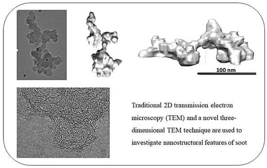
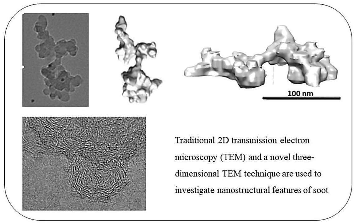
Nevertheless, TEM (transmission electron microscopy) and HRTEM (high-resolution TEM) are the most widely accepted and recognised methods to characterise soot nanostructure and morphology [
15,
19]. The other procedures mentioned above are used in most of the cited literature mainly as a complementary method to support TEM analysis. The HRTEM is a technique that relies on the very small electrons’ wavelength (2.5 pm at 200 kV with respect to 400–700 nm of light) to observe objects only a few nanometres in size as soot nanoparticles [
20]. It allows taking images of the particulate that can be subsequently further processed. For this task, a MATLAB script can be used to calculate the particles’ characteristics [
21,
22]. Another novel technique to examine the particulates is 3D electron tomography. This is accomplished by tilting the grid beneath the HRTEM electron beam about the sample centre axis and capturing images at successive degrees of rotation. [
23]. This technique enables obtaining an accurate measurement of the volume of fractal nanoparticles (agglomerates), overcoming the limitations of the 2D assumptions [
23]. 3D-TEM for soot is still in its early stages, but considerable progress has been made to reduce the time needed to build the tomogram and optimise results [
24]. In contrast to the more conventional 2D-TEM, this method is used in this work to evaluate what new information may be gleaned from soot particles. In general, soot particles can be differentiated into two categories: primary particles and secondary particles [
25]. The primary particles are typically quasi-spherical particles made up of a core, a shell, and in some cases, an amorphous layer; the secondary particles are aggregates of these primary particles [
25]. Many carbon lamellae (i.e., fringes), arranged in ordered (basic structural unit, BSU) and disordered regions, constitute the primary particle. The features of these fringes have an impact on the particles’ reactivity [
25,
26]. The main parameters are the fringe length (extent of carbon layer), fringe separation (distance between two lamellae), and fringe tortuosity (ratio of length to fringe end points closest distance) [
26]. A shorter fringe, higher separation and greater tortuosity lead to greater reactivity levels [
26]. Reactivity makes the particles easier to burn away and oxidise but also more dangerous for biological interactions once inhaled inside the lungs [
26]. On the other hand, the agglomerates’ features are the skeleton length (LSK), the skeleton width (WSK), fractal dimension (Df) and aspect ratio (LSK/WSK) [
25].
The formation of these particles, which take on various shapes and morphologies, is generally poorly understood because of the extremely complex hydrocarbon chemistry during combustion [
8]. Overall, soot formation is split into five stages: nucleation, mass growth, coagulation, carbonisation, and oxidation [
10,
27]. Nucleation concerns the accumulation of predecessor particles that convert the molecules into particulate systems. Soot inception has been directly related to the formation and growth of polycyclic aromatic hydrocarbons (PAHs) [
10,
27,
28,
29]. The formation of C
2, C
3, and C
4 hydrocarbon groups (e.g., C
4 means 4 atoms of carbon in C
4H
x) and their subsequent reaction with the first aromatic ring C6 (benzene) molecules have each been identified as the primary source of PAHs [
10,
27], which then increase through the HACA mechanism (H abstraction and acetylene addition) [
30]. Additional formation mechanisms are also postulated, with more details provided in the literature [
10,
27,
29]. Early soot agglomeration/aggregation followed by carbonization/graphitisation have been detected, suggesting the occurrence of early coagulation and clustering of small aromatic radicals [
30,
31] that are likely to eject radicals detected by LDI-TOFMS analysis at high laser power [
32]. This confirms that there are still some uncertainties surrounding the subject. It has been suggested that mass growth follows the same track as the nucleation process, as further PAH condensation through the HACA mechanism adds more carbon to the particle [
10,
27], allowing an increase in size. Coagulation occurs as the growing soot particles stick together in larger clusters and bundles [
10,
27], creating secondary particles. Mass accumulates, and due to surface growth, rounding occurs. Carbonisation essentially describes the phenomenon of soot conversion from amorphous to graphitic carbon material [
27]. Oxidation involves the reaction of oxygen with soot at high temperatures, burning away the particles. Details about oxidation mechanisms are not accessible yet, as the exact soot compositional features are not deeply understood [
10].
Further work is needed to understand the effect of the fuel type, combustion design, and temperature on soot generation; this paper focuses on the first aspect, observing what type of soot forms from two chemically different fuels. The nanostructural features are investigated with classical 2D and novel 3D TEM techniques.
2. Methodology
Soot samples were collected in premixed laminar flames at atmospheric pressure at different HABs [
15]. Premixed flames of ethylene/oxygen and benzene/oxygen mixtures, the latter one diluted with 77 vol% nitrogen, were stabilised on a McKenna burner (Holthuis & Associates, Sebastopol, CA, USA) with different equivalence ratios (2.4 and 2.0, respectively) and different cold gas velocities (4 cm/s and 3 cm/s, respectively) to achieve comparable maximum flame temperatures (1770 K and 1720 K, respectively). Specimen label was initiated by burning ethylene (E) and benzene (B) fuels followed by the value of the HAB, e.g., samples B6, B10 and B14 were collected at different heights above the burner: 6 mm, 10 mm and 14 mm, respectively. These requirements are essential for analysing how the particles form in optimal lab settings and for understanding which factors have the greatest impact on the nanostructure. More details on the flame and sampling systems are reported elsewhere [
13,
14,
15]. Adsorbed organic species were removed from soot by dichloromethane extraction. The thermogravimetric analysis (TGA) was carried out on a Perkin-Elmer Pyris 1 thermogravimetric analyzer (Waltham, MA, USA). The maximum oxidation temperature was evaluated on the TGA profiles measured by heating soot samples from 30 to 900 °C in air flow (30 mL × min
−1). The hydrogen to carbon (H/C) atomic ratio of soot was measured by a Perkin-Elmer 2400 CHNSO elemental analyzer.
In this work, the main objective was to characterise the soot particle structure. Sample preparation involved soot dispersion into ethanol by an ultrasonic bath at room temperature for 20 min, for contamination removal and particle separation. Subsequently, the soot specimens were placed on the graphene oxide-coated copper mesh grid. The ethanol evaporated immediately, leaving only the particles. The grid was analysed under a “JEOL 2100F” TEM (Tokyo, Japan) equipped with a Gatan Orius CCD camera (Gatan Inc, Pleasanton, CA, USA) and magnifications up to 600,000× providing. This experiment methodology and the sample preparation were applied using previous literature works as compliance benchmarks [
14,
21]. Ethanol was used as a solvent to better disperse the particles, as also suggested in [
15], although other methods using a different dilution approach have also been explored [
14,
21]. Morphology, primary particles’ diameter, and reactivity were investigated. The ImageJ software was employed to measure the primary particles’ sizes. Subsequently, a MATLAB algorithm was adopted to calculate the dimensions and analyse the fringes of the particles. This technique is described in more detail in [
21,
22] and is not discussed here for brevity, but essentially, regions from the TEM images are selected to compute the nanostructure features of the carbon lamellae (length, tortuosity, and separation).
For the 3D TEM, 10 nm diameter gold nanoparticles were added onto the copper mesh grid to allow particles’ alignment, again using the “JEOL 2100F” TEM. Tilt series of ±60 degrees, at 1-degree steps, were then acquired to reconstruct the tomogram employing IMOD software and backwards projection. Once the 3D model was generated, both qualitative and quantitative analyses were performed. The first one focused on the new structural features that can be ascertained from observation; the second focused on volume and surface area calculations, which can then be compared to 2D ones. 3D volume and surface area measurements were taken by using the ImageJ BoneJ plugin [
33]. On the other hand, the 2D ones use the method described by Orhan et al. [
34], which estimates the number of primary particles from the equation developed by Neer et al. [
35].
where
,
[
35],
Aeff is the projected area of the particles and
Ap is the assumed representative primary particles’ cross-sectional area, calculated from the average diameter (
dp). Then, 2D volume and surface are estimated as:
3. Results and Discussion
An overall description of soot samples is given in
Table 1, reporting the TGA temperature at the maximum oxidation rate (T
max), the H/C atomic ratio, and the HRTEM data as the inter-plane distance, d, and the aromatic layer size, L. The very small amount of B6 sample allowed to perform only HRTEM analysis.
It can be observed that soot becomes less reactive and hydrogenated with ageing, as demonstrated by the T
max rise and the H/C decrease. Consistently, the ageing has an effect also on soot nanostructure with the increase in L, whereas d remains constant.
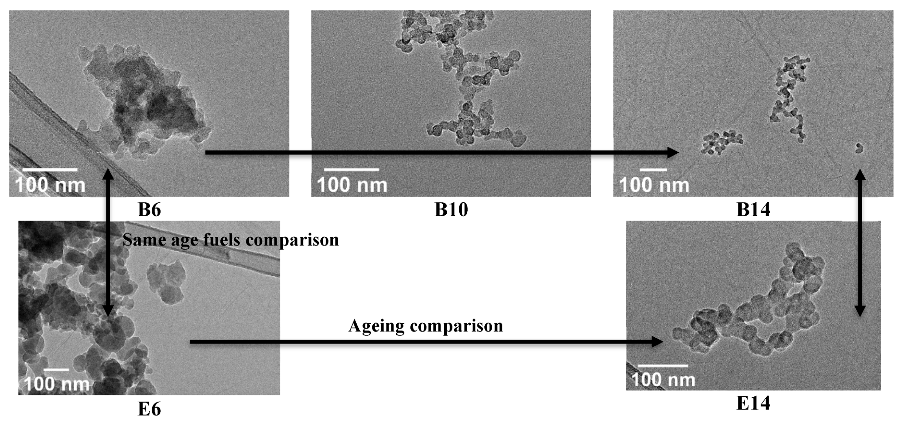
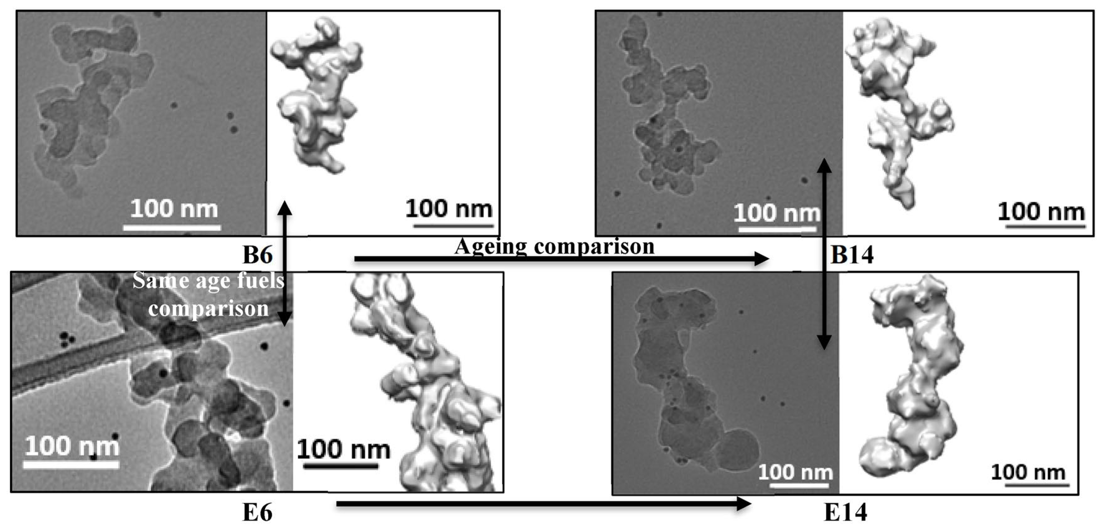
Figure 1, reporting the TEM images of soot, shows how, in the ageing direction, the soot particles tend to go from bundle/cluster agglomerates to chain-like structures.
The trend is similar for both E and B particles and related to the amorphous nature of the young particles, which have a higher presence of reactive sites and easier coagulation/oxidation, as also found by Uy [
16] and Vander Wal [
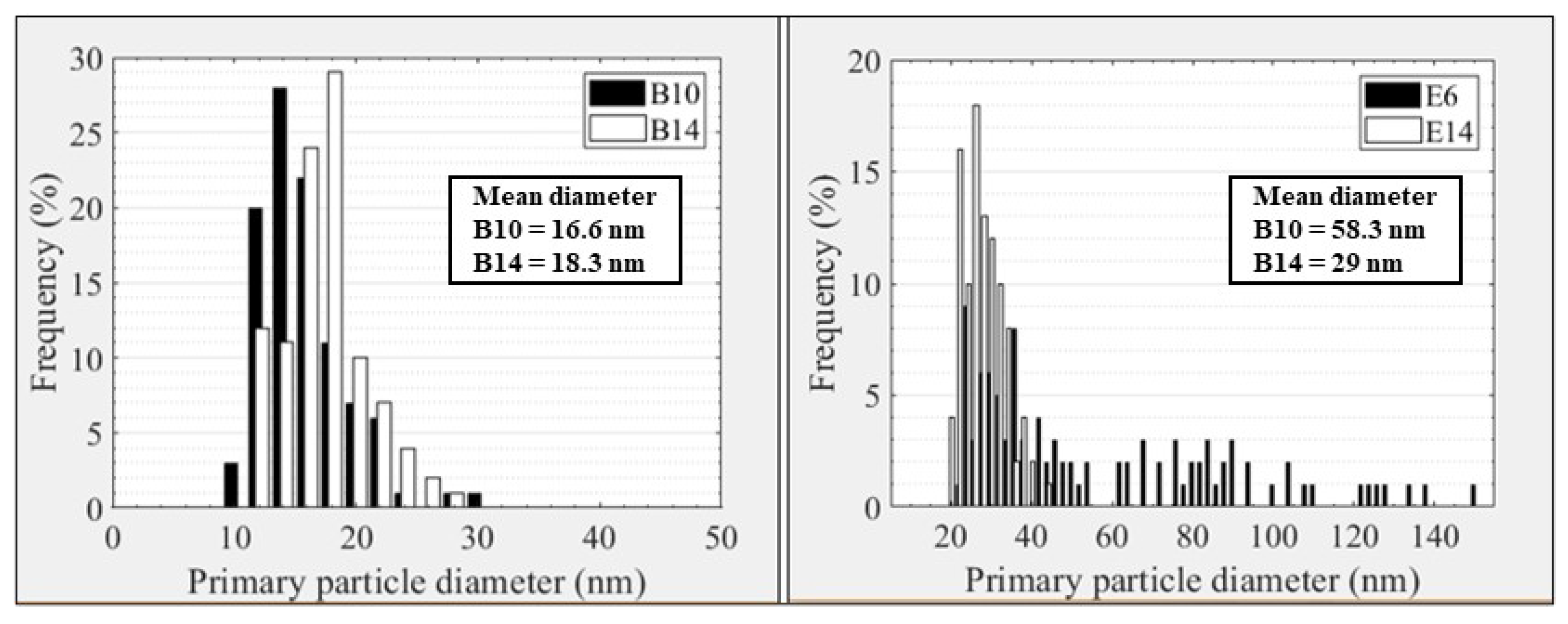
36]. The primary particles’ diameter distribution per sample was measured, and the results are presented in
Figure 2. B6 size could not be assessed due to the cluster nature of the soot, which hindered the detection of sufficient well-defined primary particles. From
Figure 2, it can be noticed how soot size increases with ageing for B but reduces for E. Specifically, 97% of the B10 particles are between 10 nm and 23 nm, with a mean value of 16.6 ± 3.6 nm, whereas the B14 particle size distribution is slightly shifted to a larger size, with 96% of the diameters being between 12 nm and 24 nm and a mean of 18.3 ± 3.4 nm. E6 has a larger size distribution, ranging from 23 to 155 nm, with a mean of 58.3 ± 32 nm. E14 has 93% between 21 nm and 38 nm, an average of 29 ± 5.1 nm. This decreasing size suggests that ethylene soot is oxidising more quickly than benzene, consistent with the TGA analysis (
Table 1).
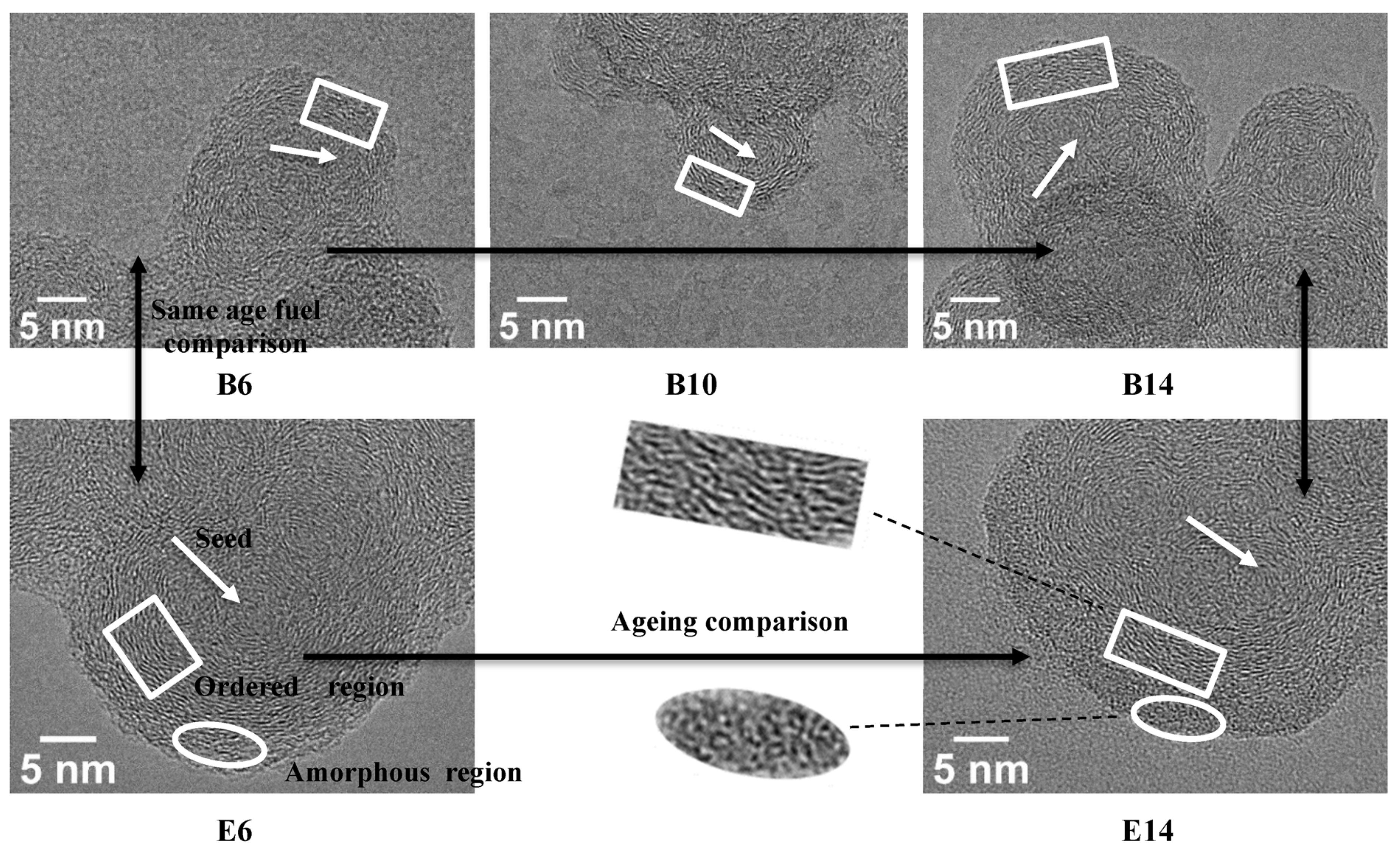
The particles’ nanostructure is presented in
Figure 3. In general, some graphitisation of the fringes (stacked ordered carbon lamellae in the shell) is present in all the samples (square boxes in
Figure 3). The “ageing” effect shows an increase in the degree of graphitisation and concentric stacking of the lamellae around the onion-like structure seeds (white arrows in
Figure 3). The seed development augments the concentric nanostructure of the fringes in the mature soot. Meanwhile, comparing vertically the two samples at the same “age”, a thicker amorphous layer (oval box in
Figure 3) is observable at the edge of the ethylene particles in contrast to the benzene ones. This thick, disordered region would explain why E is burning more quickly than B, as also found by Russo et al. [
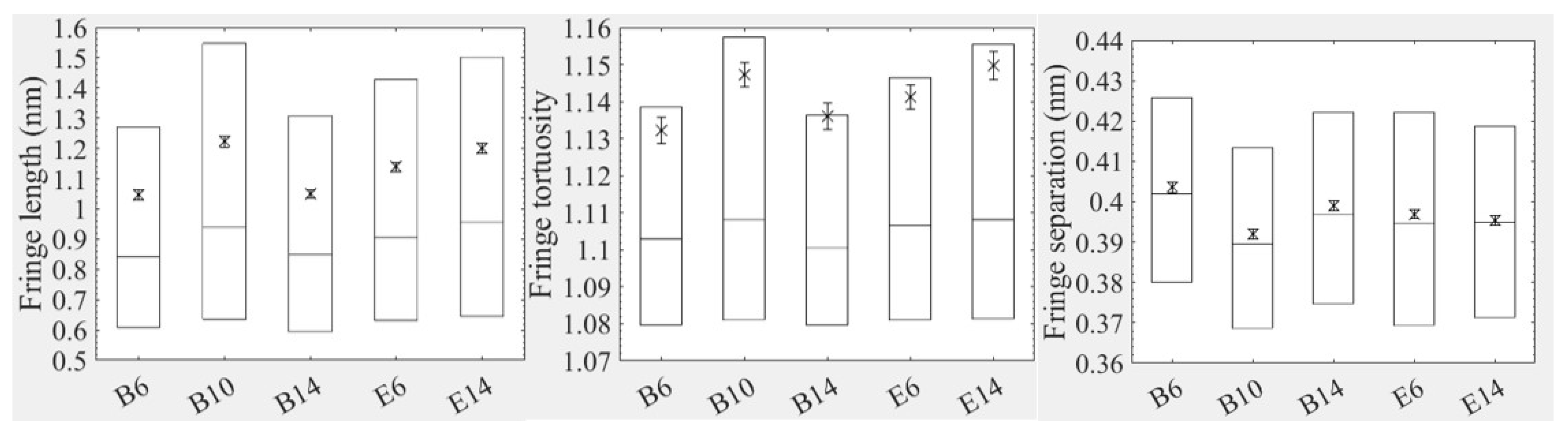
37]. To have a more quantitative analysis of the nanostructure, 2000 fringes have been selected from the TEM images and measured with the aid of a MATLAB algorithm. This allowed producing a comparison of all 5 samples with respect to their fringes’ length, tortuosity, and separation (reactivity characteristics). These results are shown in
Figure 4. The fringe length tends to grow with ageing soot, from 1.04 nm of B6 to 1.22 nm of B10 to 1.05 nm of B14 and from 1.139 nm of E6 to 1.20 of E14 (±0.002). Tortuosity does not vary greatly, ranging between 1.132 and 1.147 for benzene and between 1.136 and 1.149 for ethylene (±0.004) (error bars with STD in brackets). Separation is also quite similar across the samples, with 0.404 nm of B6, 0.392 of B10, 0.399 nm of B14, 0.397 nm of E6 and 0.396 nm of E14 (±0.002). Similar nanostructure results were also obtained by Apicella et al. [
15].
Following the 2D TEM analysis, a 3D TEM investigation was also carried out. Only four 3D particles in total, one for each of the four samples (B6, B14, E6 and E14), were produced overall due to time and financial constraints. The distribution and quantity of the golden particles around soot particles on the grids served as the deciding factors in choosing these particular particles as opposed to those shown in
Figure 1 for the 3D reconstruction. For the 3D to be executed, the number of gold particles needs to be adequate. Regrettably, their location is not easy to control. The model generated in 3D was then compared to the respective 2D TEM image (untitled) to understand the differences in the information achievable with the two methods. A qualitative analysis can be performed by looking at the 2D images at a 0° tilt angle together with the 3D models at roughly the same orientation (
Figure 5).
Table 2 summarises the geometrical characteristics of all the particles and compares the 3D and 2D results. The 3D parameters are calculated using the ImageJ BoneJ plugin [
33], while the 2D parameters are calculated by utilising Equations (1)–(3). It can be noticed that the 3D volume is much larger than the 2D estimation, while the surface area is lower. This emphasises the uncertainty surrounding the 2D projections’ ability to accurately capture the shape and structure of agglomerates. The morphology results can vary significantly with modifications to projection angles. This was shown by Adachi et al. [
38], where 2D-derived properties were proven to be sensitive to changes in angle. The wide range of measured values found in studies often illustrates the significant uncertainty in 2D approaches. For instance, Rogak et al. [
39] found an underestimate of about 10–20% of the fractal dimension by 2D projections, while Martos et al. [
40] obtained a fractal dimension overestimate. On the same note, Orhan et al. [
34] observed a 54% variation in surface area and a 60% variation in the number of primary particles, depending on the tilt angle used. With a 3D reconstruction, the correction factors can be avoided, and the characteristics of the soot shape can be much more accurate, as also supported by Van Poppel et al. [
41]. Baldelli et al. [
42] reported a 6% error in the projected area equivalent diameter (PAED), albeit the projected area and PAED are two different quantities. The first is the 2D projection of the surface area. Instead, PAED is derived from the conversion of the surface area into a sphere, whose 2D projection circle diameter is measured. This may cause some error bias, as the diameter has to be squared to compute the surface area of the circle. For example, if two diameters that are 6% apart are considered (94 and 100 nm), the two corresponding areas’ percentage difference is:
Therefore, for the area, the error is higher (here it doubled), as it is the square of the diameter.
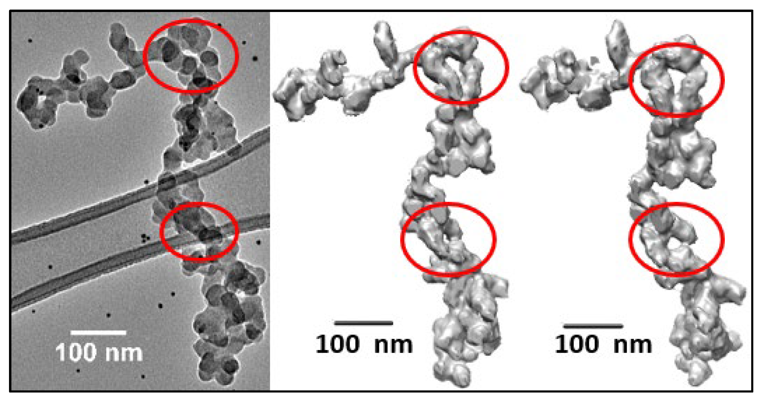
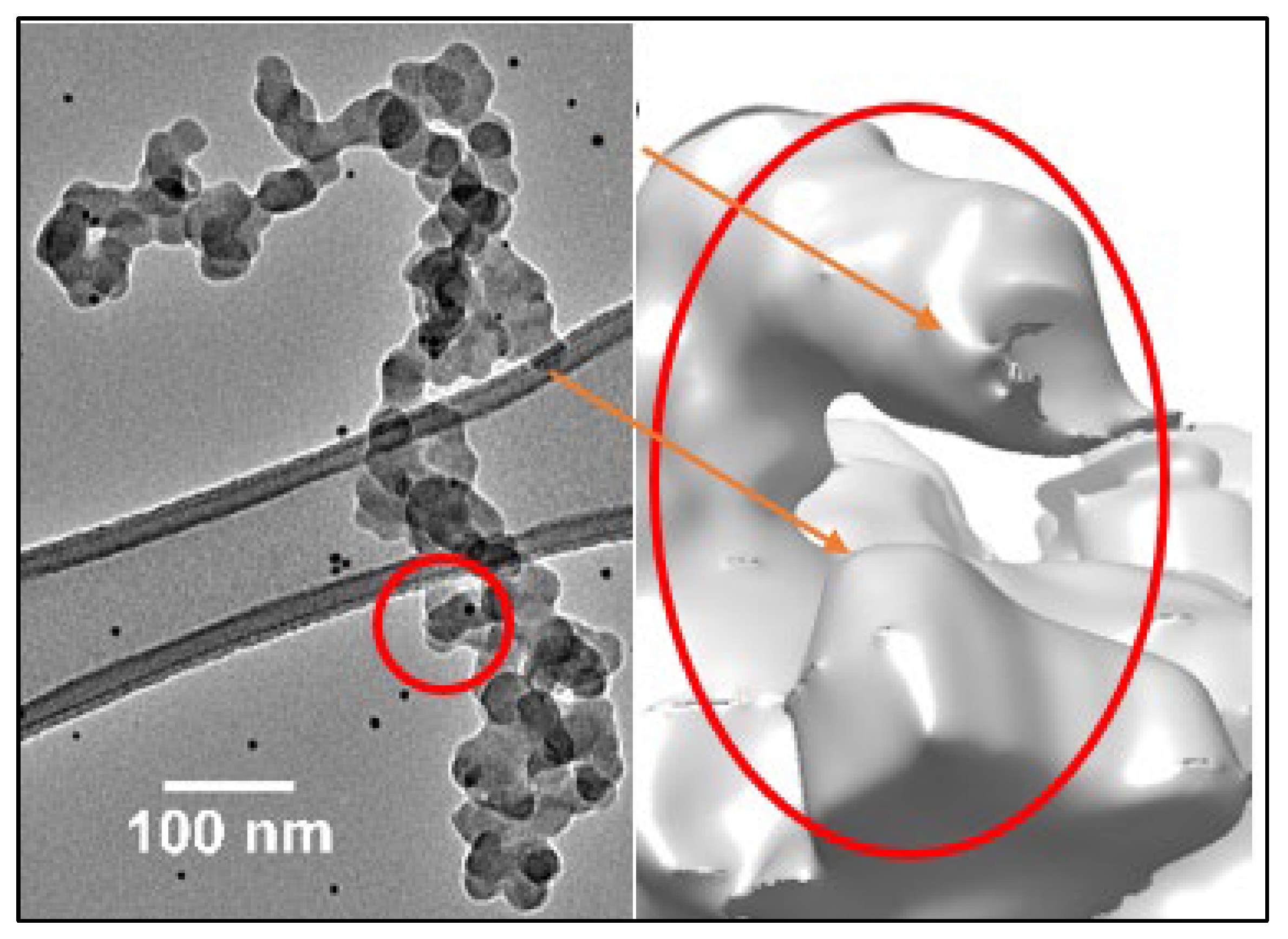
The main benefit of 3D models is the ability to see structural details that may be hidden in 2D. The E6 particle chosen provides the greatest illustration of this advantage. Just by rotating the particle (
Figure 6) by a few degrees, it is possible to detect ring structures, a characteristic also reported by Baldelli et al. [
42], which may be related to the formation mechanisms of the soot. By minimising overlaps that could conceal other features, 3D models also help with a better understanding of the spatial location and position of the primary particles. For instance, while still focusing on E6, the rotation allowed observing an additional primary particle that would have otherwise gone unnoticed (
Figure 7). Moreover, the “C” shape of the particles on top is noticeable. By angling the image, in another investigation, it was possible to recognise that one primary particle was not a part of the main agglomerate [
34]. Understanding the third dimension is undoubtedly another benefit of the 3D model.
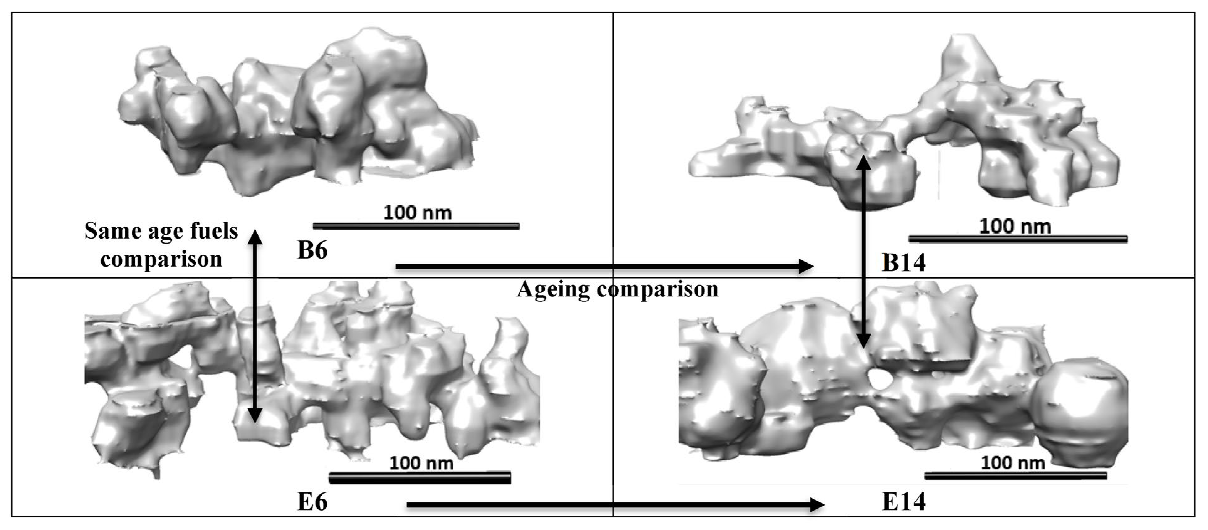
Figure 8 demonstrates how in the third dimension, the particles may vary substantially. The 3D allows the distinction of gaps and holes present in the bulk of the particles, and this is evident in B14, E6 and E14. In B14, for example, from the 2D picture in
Figure 5, it is not possible to know that the two lumps of soot at the two ends of the particle, joined by a small chain, are on two different planes. In addition, the shape of the primary particles can be better analysed, remarking that they are not perfect spheres but rather oval shapes.
Looking at the aggregates reported in
Figure 8, primary particle growth and the cluster-to-chain agglomeration pattern appear to be in contradiction with the 2D results. For example, in 3D, the ageing of benzene soot gives smaller particles and the ageing of ethylene soot gives larger diameters. In addition, E6 and B6 samples have a more elongated structure in comparison to the 2D analysis. However, since only one particle per sample was examined in this study and that particle might have come from anywhere in the diameter distribution shown in the histogram in
Figure 2, a more thorough investigation is necessary.
4. Conclusions
The study of flame-generated soot samples from two fuels—benzene and ethylene—was carried out, focusing on the morphology and nanostructure of the aggregates. In order to analyse the samples’ morphology, primary particles’ size, reactivity (2D) and geometrical features (3D), 2D and 3D techniques were used. The 2D results revealed that the morphology changes from a cluster-like to a chain-like structure as the soot ages.
The ethylene particles’ diameters are larger than the benzene’s, and, generally, the size increases with older soot. This can be related to the fact that aromatic molecules and freshly nucleated soot particles persist in aliphatic flames, also downstream of the flame. This freshly generated amorphous carbon coalesces onto the particles, increasing their size [
43].
Ordered stacked carbon lamellae regions are observable throughout the specimens. This graphitisation increases with more mature samples. The most evident difference is the presence of a thick amorphous layer at the edge of the ethylene particles that is not visible on the benzene ones. Fringes’ length grows from 1.04 nm of B6 to 1.22 nm of B10 to 1.05 nm of B14 and from 1.14 nm of E6 to 1.20 nm of E14 (±0.002 nm). The tortuosity is similar across all the samples, ranging between 1.132 and 1.149 (±0.004). Separation is 0.404 nm for B6, 0.392 for B10, 0.399 nm for B14, 0.397 for E6 and 0.396 for E14 (±0.002 nm).
The 3D results allowed a more detailed observation of the geometrical structure of the agglomerates. Ring structures, particles’ overlaps, and the overall shape of the primary particles could be seen. The 3D investigation was limited in this study by the number of particles that could be considered, but the visualization of those features suggests this method can support the understanding of how, for instance, agglomerates interact with fluids and affect oil degradation in internal combustion engines. Due to the large variation in results, the 3D investigation also poses questions about the accuracy of the 2D assumptions used to calculate volume and surface area. Further development is needed in this area to improve and bring soot study to a new level.

 ,
, 


