
Development and Validation of a LabVIEW Automated Software System for Displacement and Dynamic Modal Parameters Analysis Purposes
Abstract
:1. Introduction
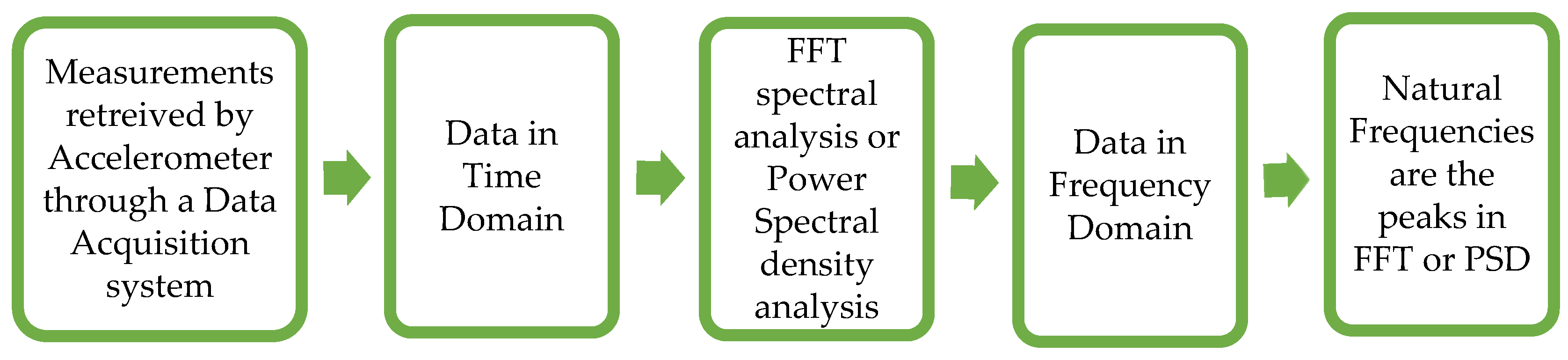
2. Natural Frequency Calculations
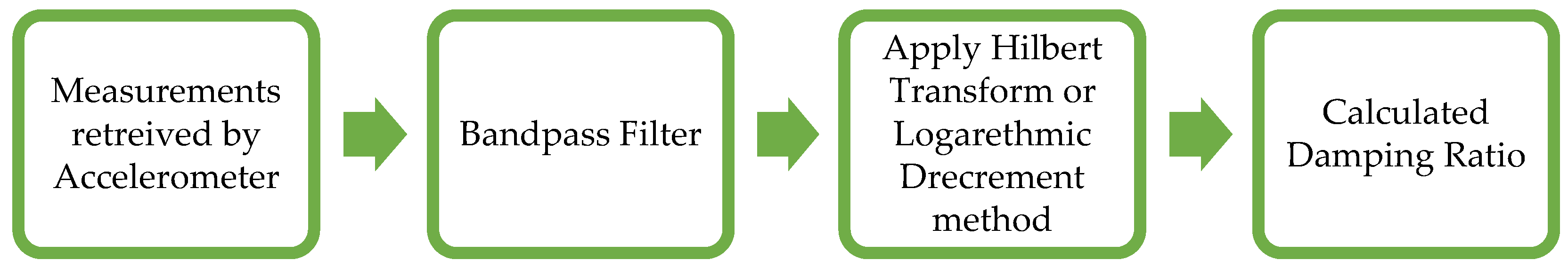
3. Damping Ratio Calculations
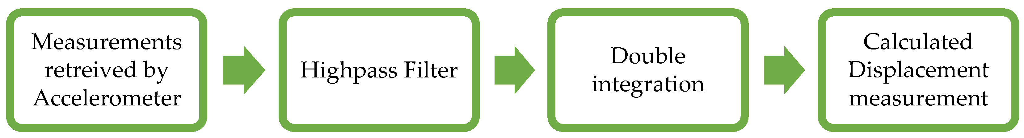
4. Displacement Parameter Calculations
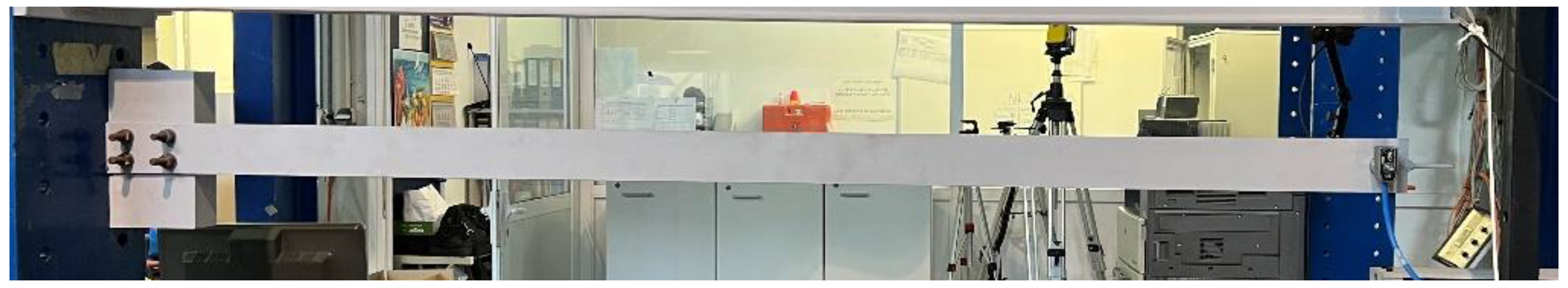
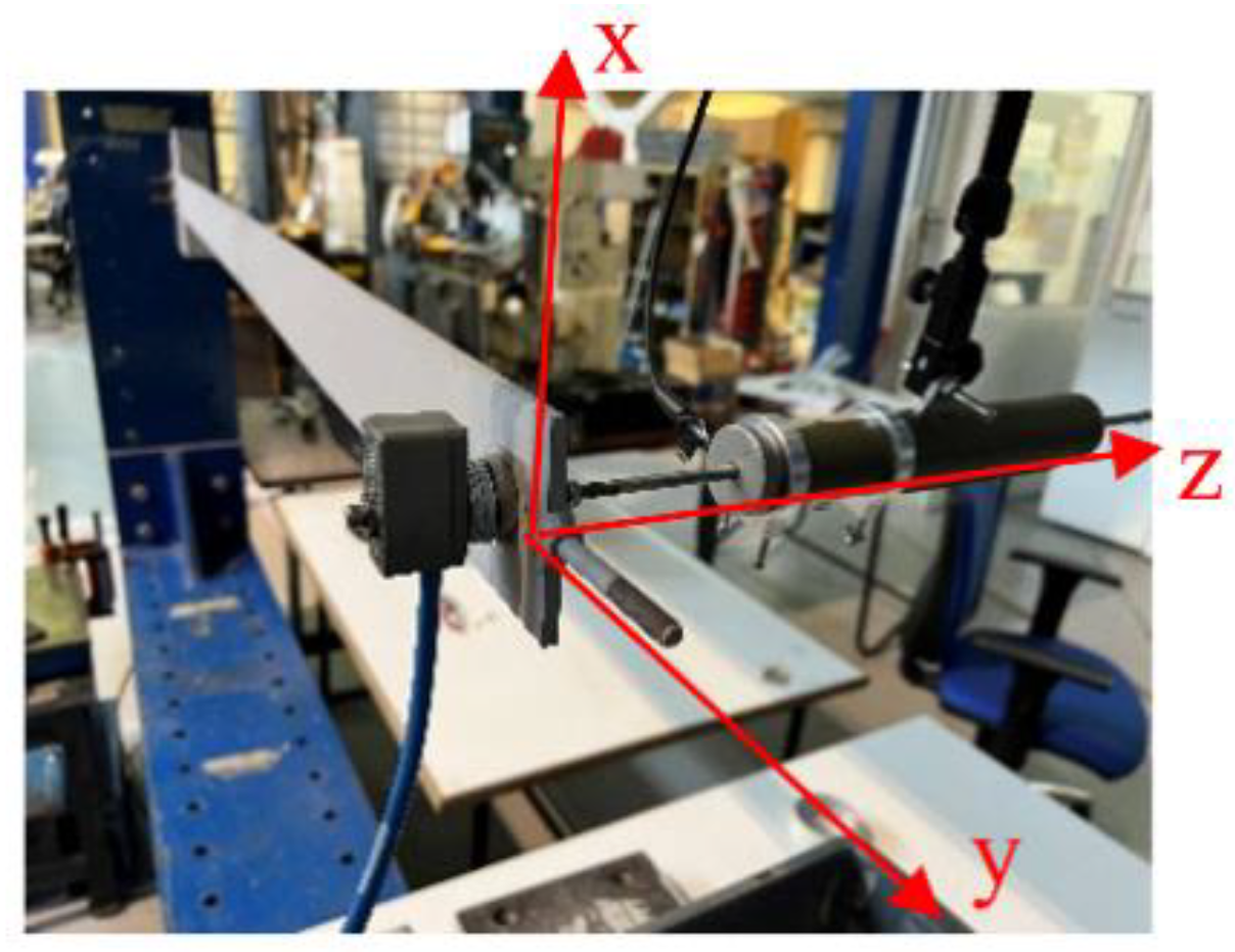
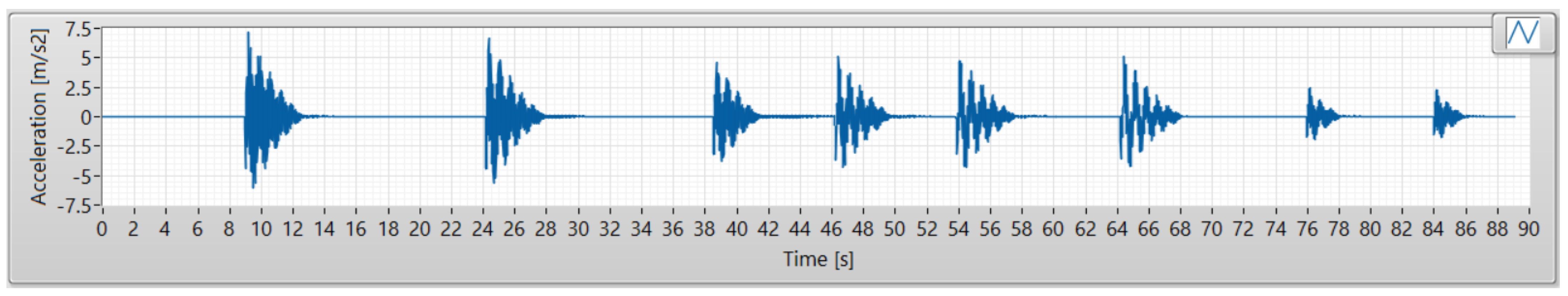
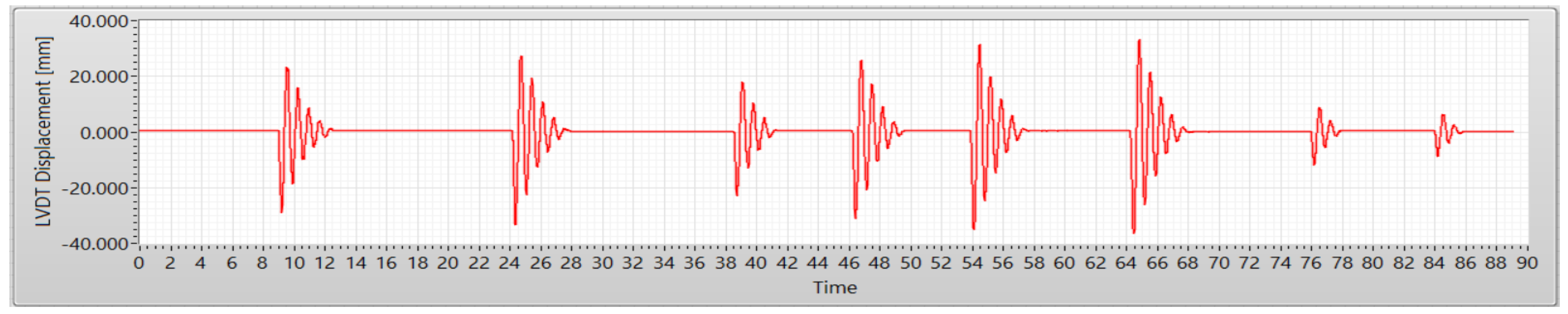
5. Experimental Benchmark Procedure
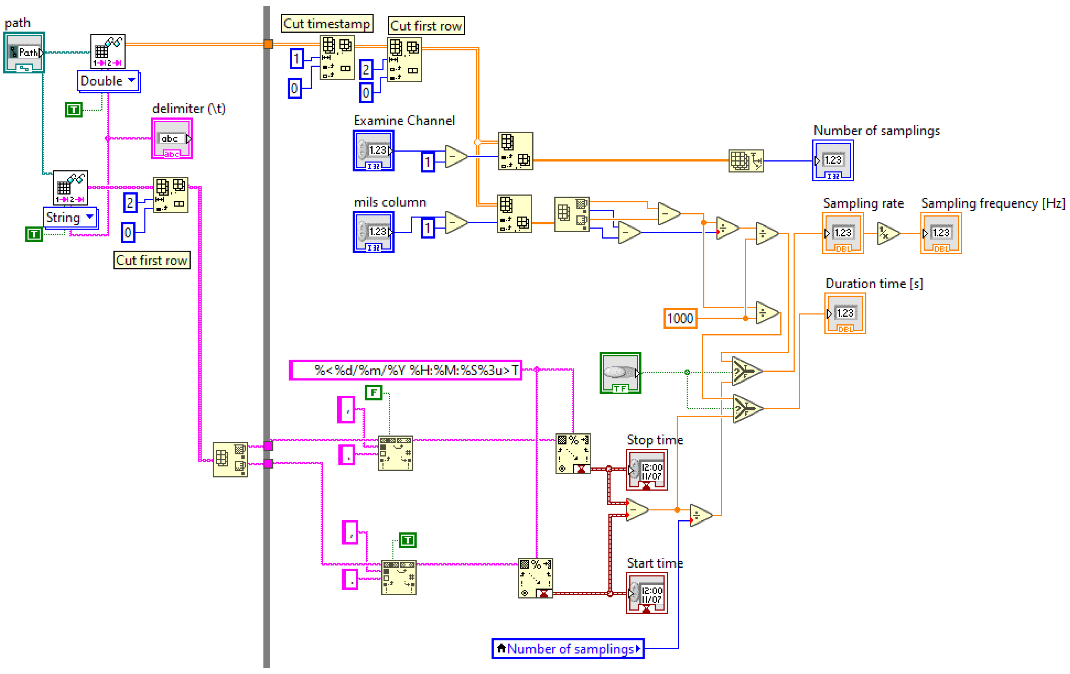
6. Developed LabVIEW Program Topology
6.1. Import the Acceleration–Time Domain Data into LabVIEW
6.2. Calculate the Mean Value and the Corrected Acceleration–Time Domain
6.3. Calculate the System Eigenfrequencies
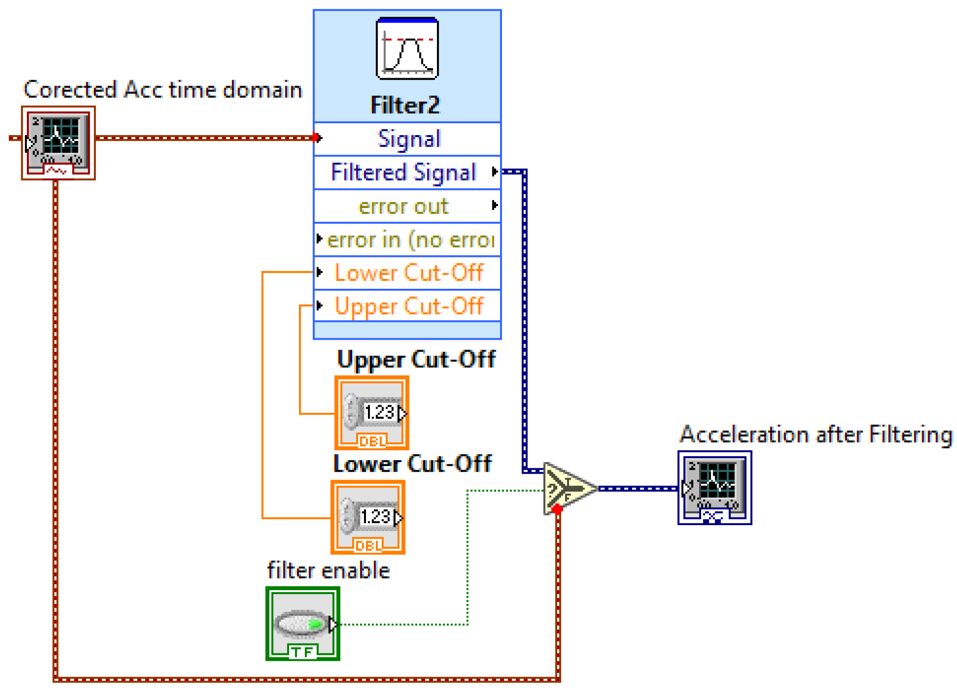
6.4. Butterworth Filter
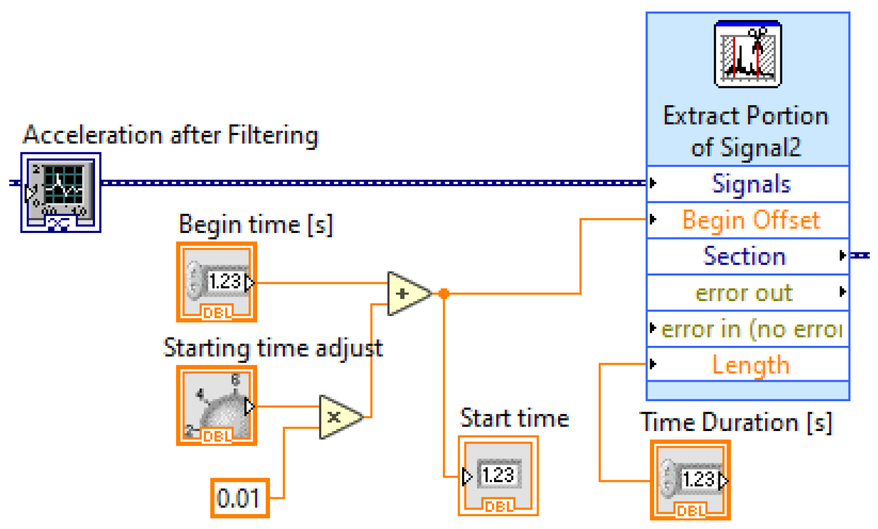
6.5. Extraction of a Portion from the Filtered Acceleration
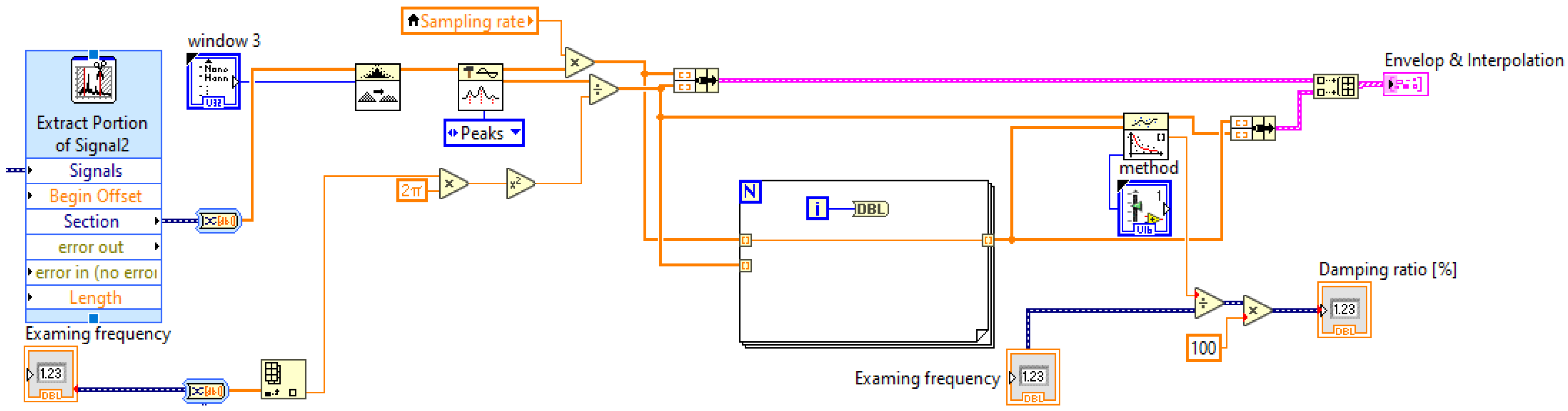
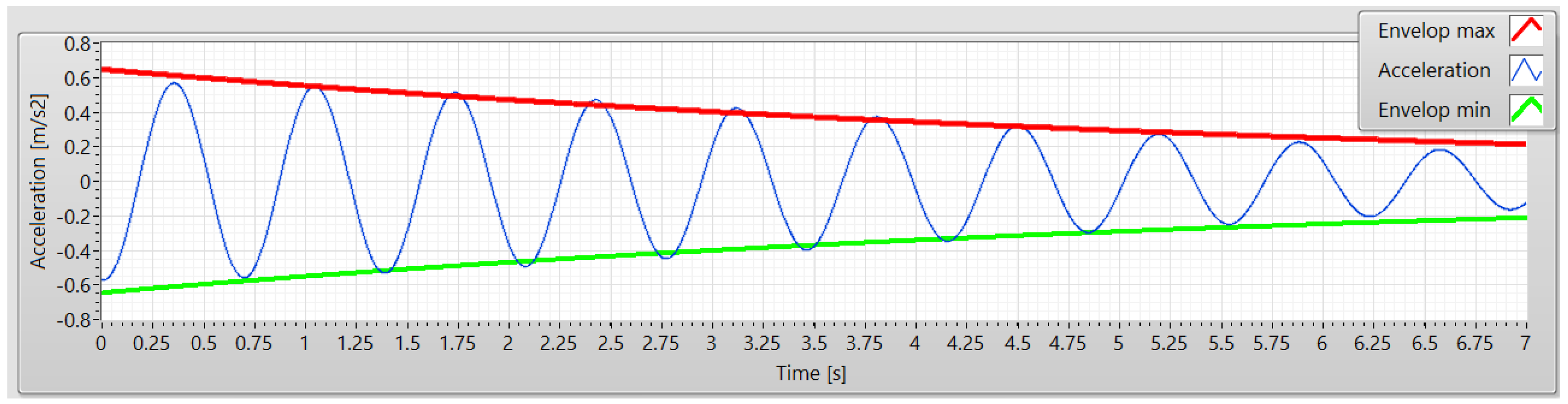
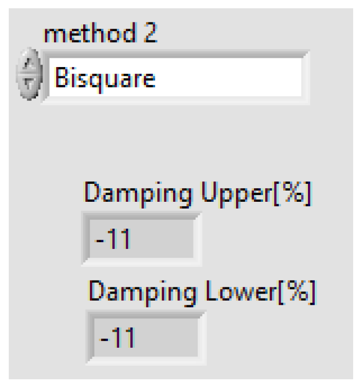
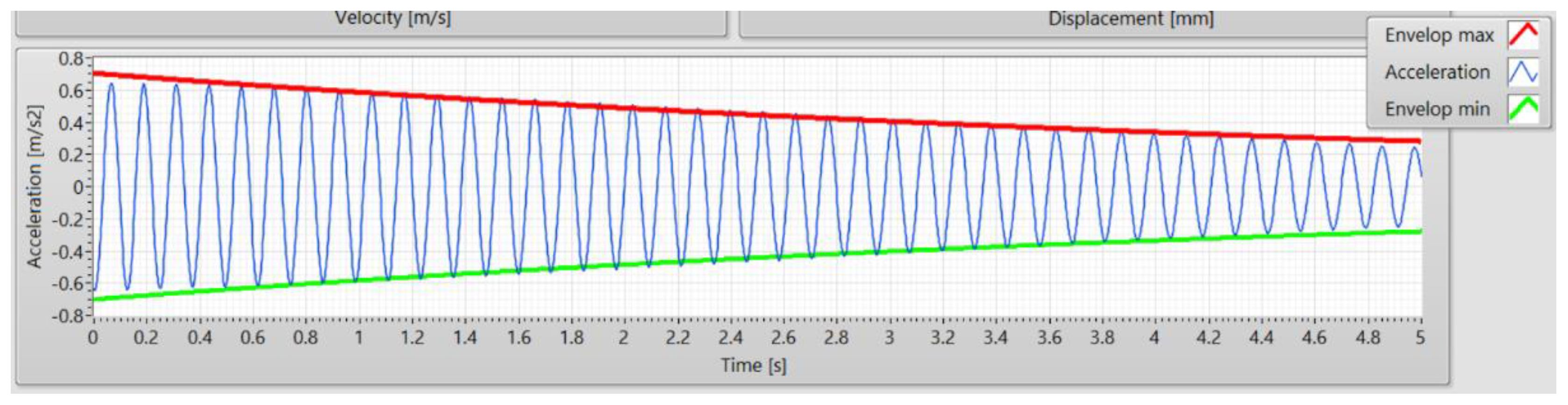
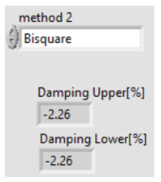
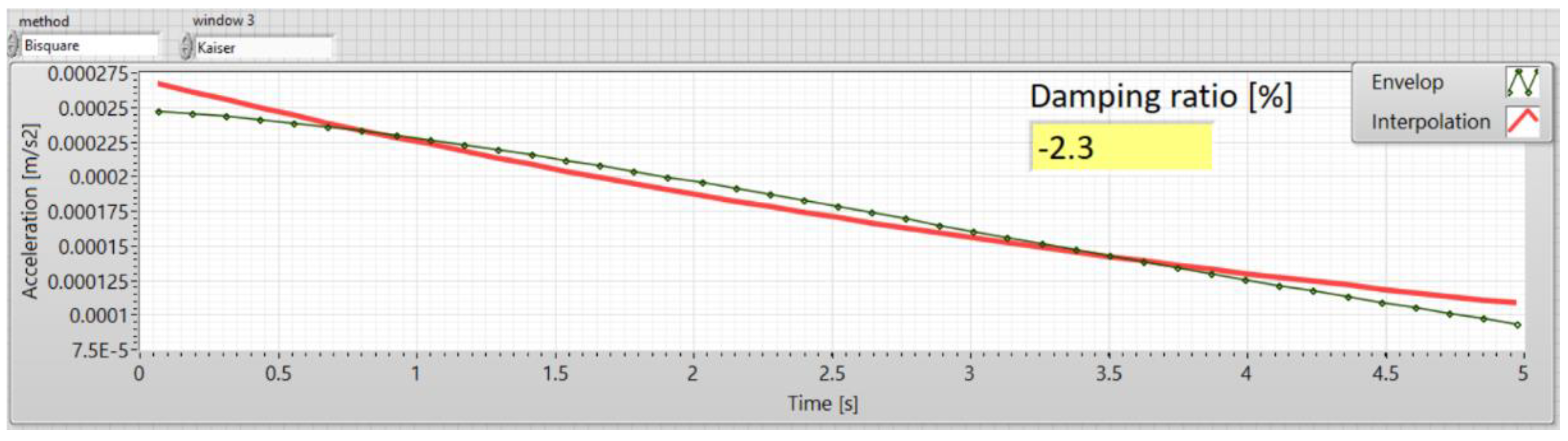
6.6. Damping Ratio Calculation
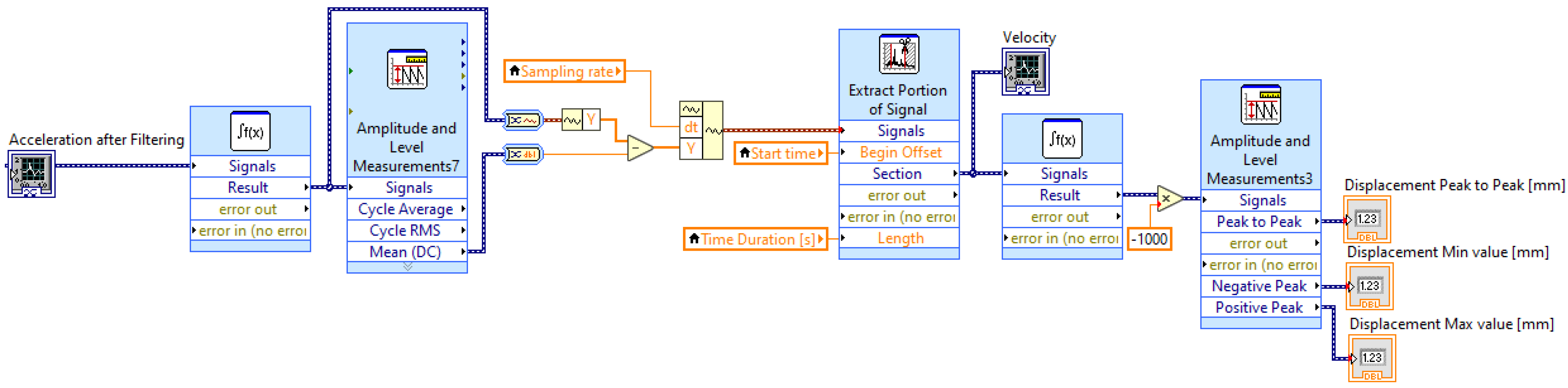
6.7. Displacement Calculation
7. Estimation of Damping Parameters
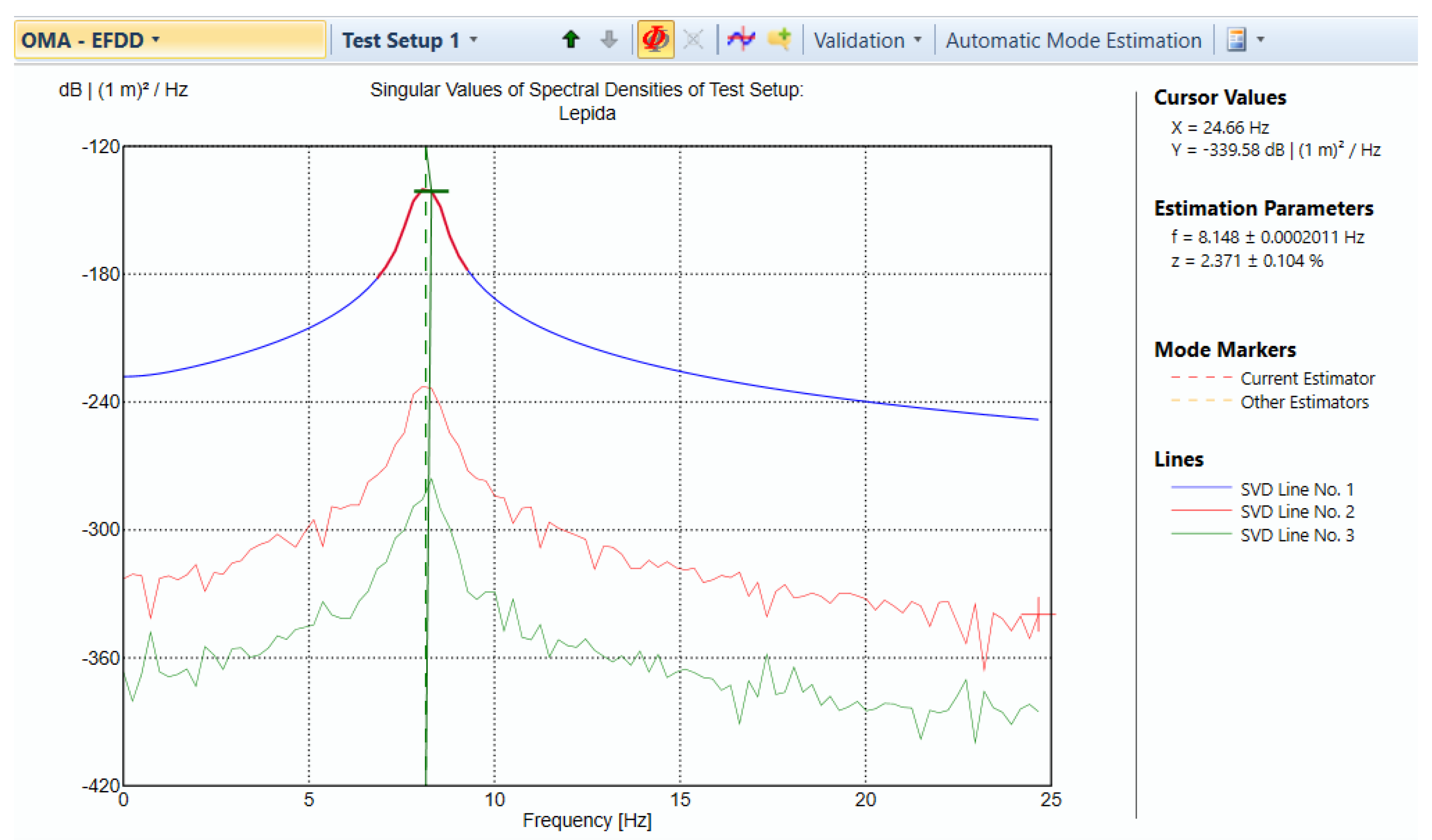
8. Benchmarking Information between LabVIEW and ARTeMIS
9. Results
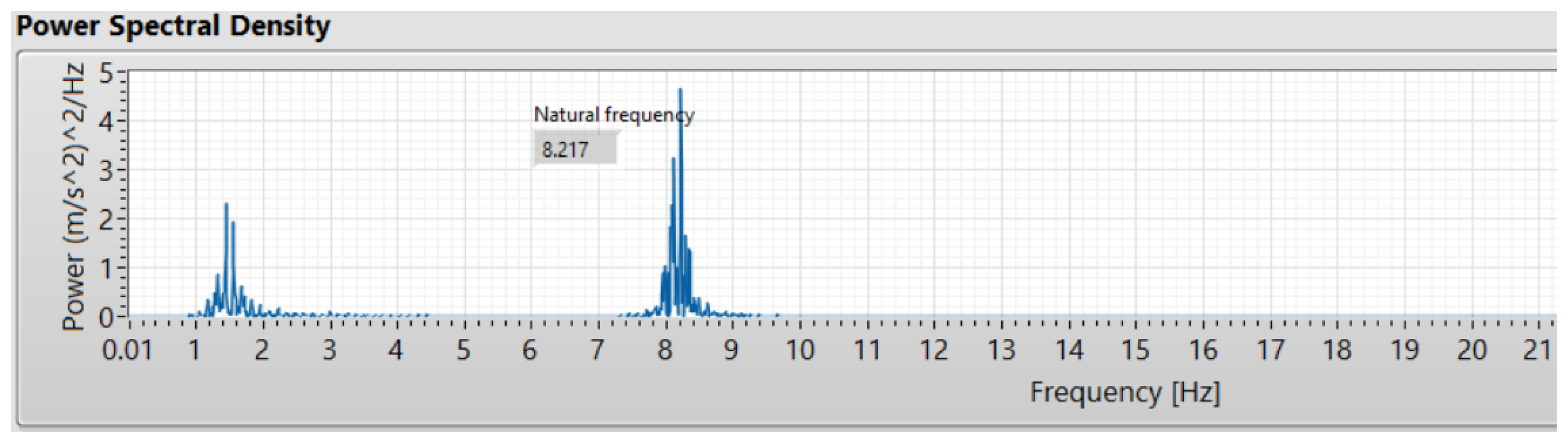
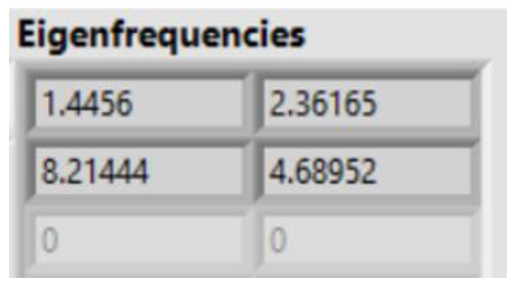
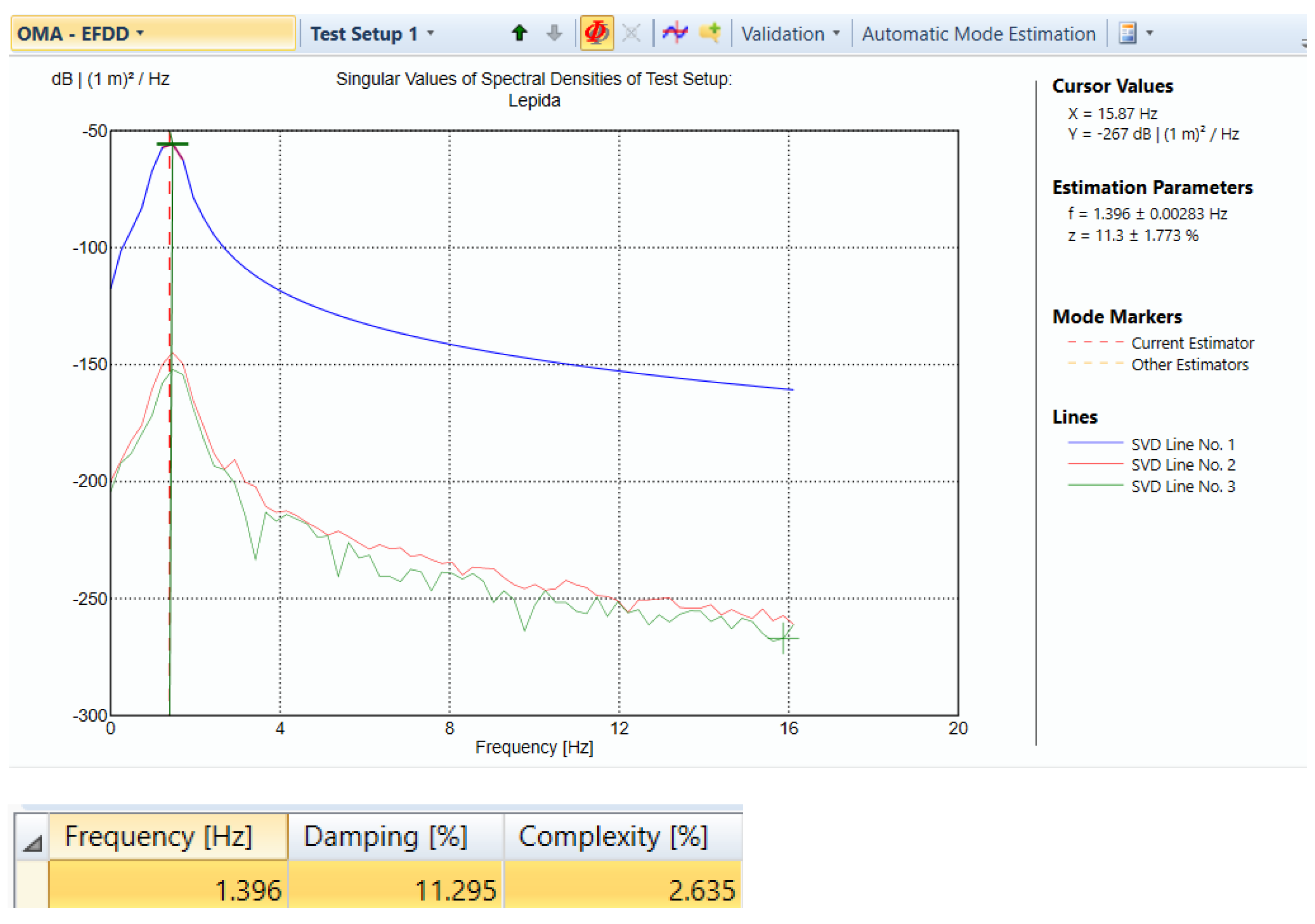
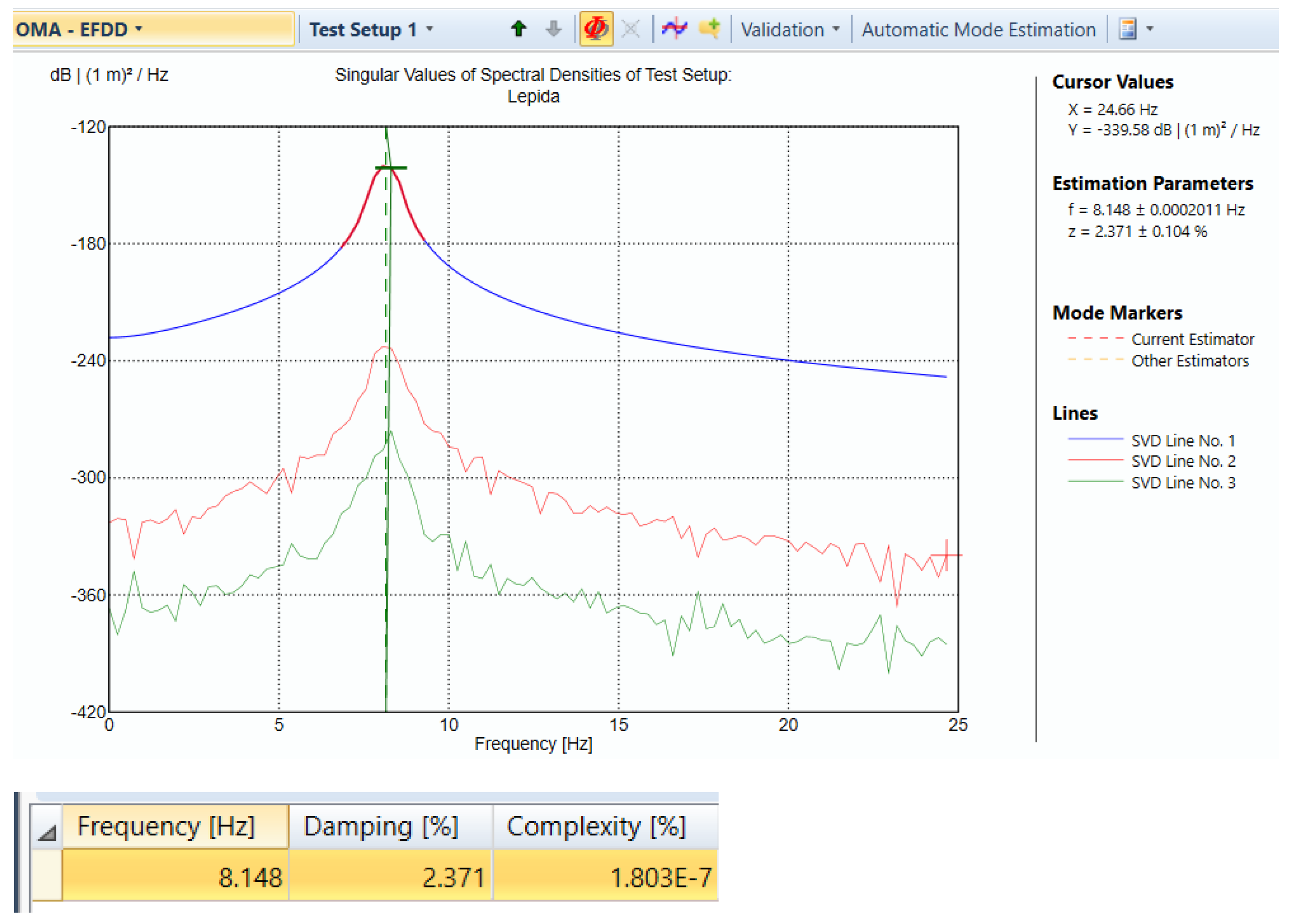
9.1. Natural Frequency
| For steel: the Young’s modulus E = 2 × 10¹¹ N/m2 |  |
| The unit weight ρ = 7850 kg/m3 | |
| b = 0.08 m, h = 0.006 m, L = 1.86 m | |
| The area: A = b × h = 0.00048 m2 | |
| The moment of inertia: I = b h3 = 1.44 × 10⁻⁹ m4 |
9.2. Damping
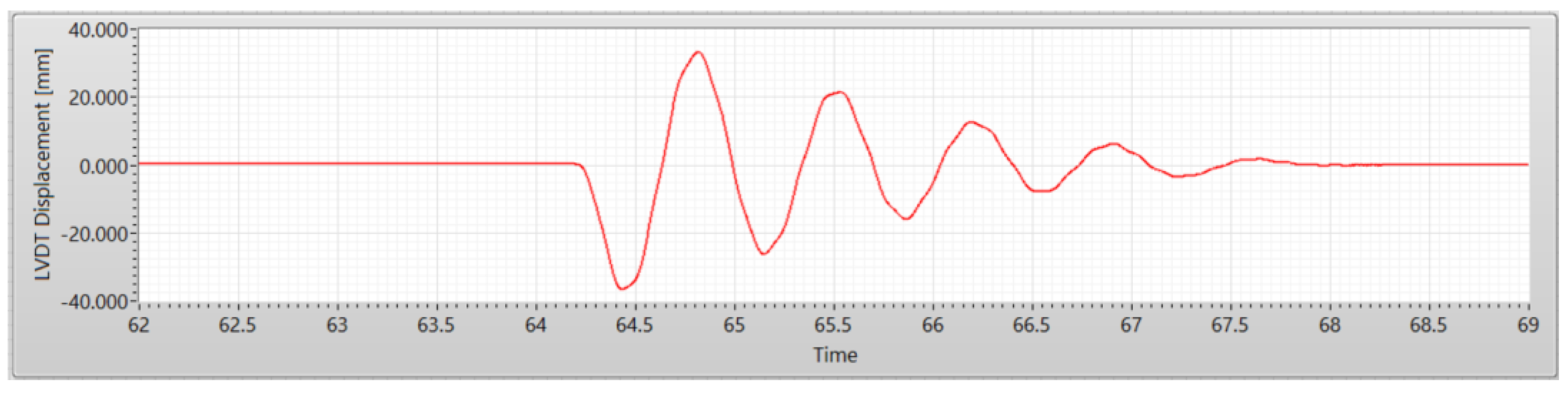
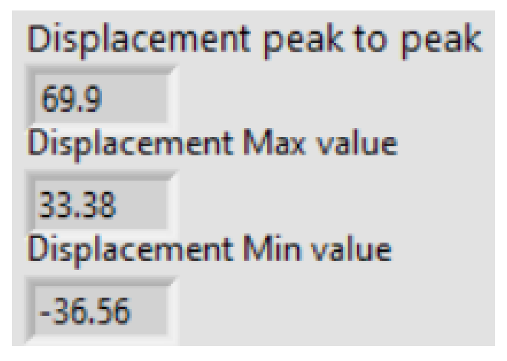
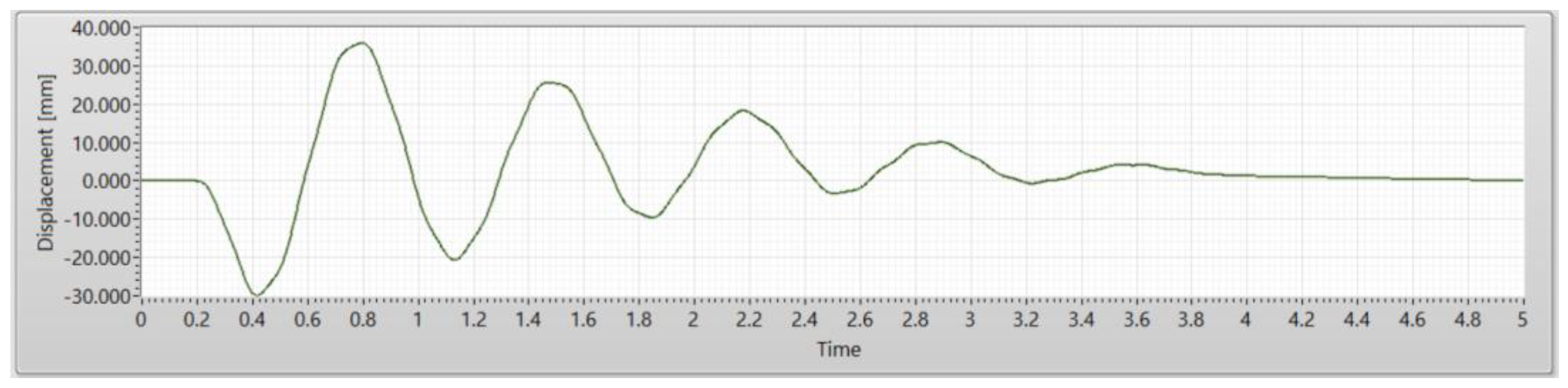
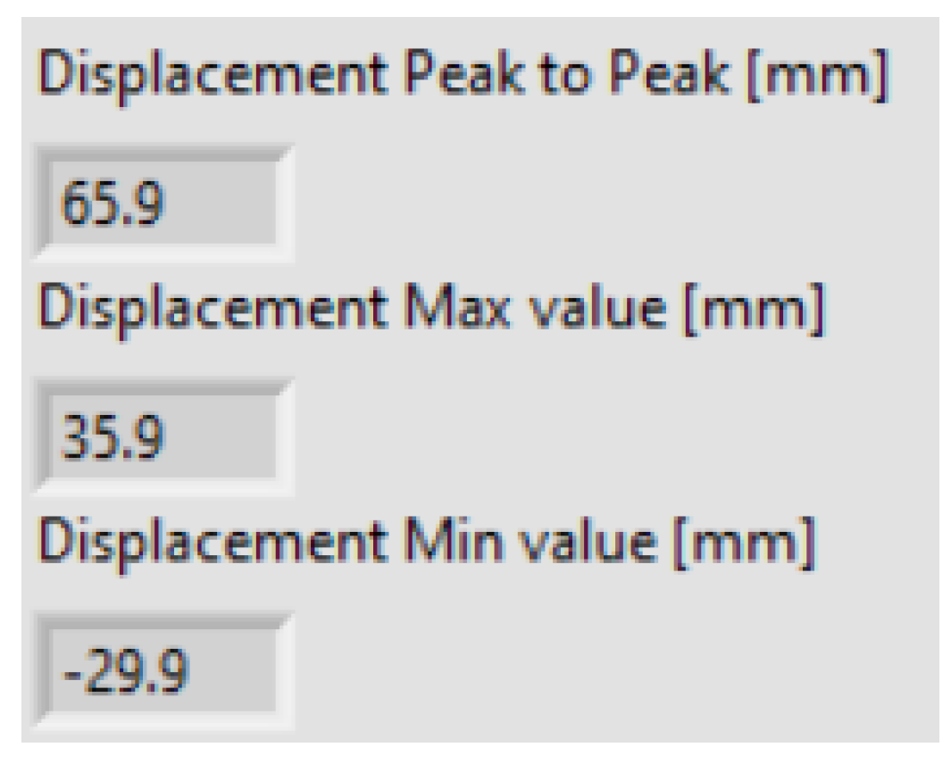
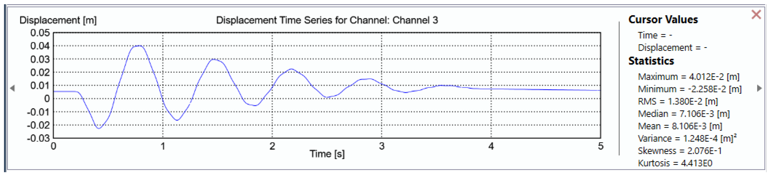
9.3. Displacement
10. Conclusions
Author Contributions
Funding
Data Availability Statement
Conflicts of Interest
References
- Badejo, E. Engineers, others urge multi-disciplinary approach to curb building collapse. Guard. Newsp. 2009, 13, 15–17. [Google Scholar]
- Lynch, J.P.; Law, K.H.; Kiremidjian, A.S.; Kenny, T.W.; Carryer, E.; Partridge, A. The design of a wireless sensing unit for structural health monitoring. In Proceedings of the 3rd International Workshop on Structural Health Monitoring, Stanford University, Stanford, CA, USA, 12 September 2001; pp. 12–14. [Google Scholar]
- Alvandi, A.; Cremona, C. Assessment of vibration-based damage identification techniques. J. Sound Vib. 2006, 292, 179–202. [Google Scholar] [CrossRef]
- Chaudhari, P.K.; Patel, D.; Patel, V. Theoretical and software-based comparison of cantilever beam: Modal analysis. Int. J. Innov. Res. Adv. Eng. 2014, 1, 75–79. [Google Scholar]
- Xia, Y.; Li, H.; Fan, Z.; Xiao, J. Modal parameter identification based on hilbert vibration decomposition in vibration stability of bridge structures. Adv. Civ. Eng. 2021, 2021, 6688686. [Google Scholar] [CrossRef]
- Wang, D.; Haldar, A. Element-level system identification with unknown input. J. Eng. Mech. 1994, 120, 159–176. [Google Scholar] [CrossRef]
- Beck, J.L.; Jennings, P.C. Structural identification using linear models and earthquake records. Earthq. Eng. Struct. Dyn. 1980, 8, 145–160. [Google Scholar] [CrossRef]
- Liu, Y.; Bao, Y. Review of electromagnetic waves-based distance measurement technologies for remote monitoring of civil engineering structures. Measurement 2021, 176, 109–193. [Google Scholar] [CrossRef]
- Lacanna, G.; Ripepe, M.; Coli, M.; Genco, R.; Marchetti, E. Full structural dynamic response from ambient vibration of Giotto’s bell tower in Firenze (Italy), using modal analysis and seismic interferometry. NDT E Int. 2019, 102, 9–15. [Google Scholar] [CrossRef]
- Bayraktar, A.; Türker, T.; Altunişik, A.C. Experimental frequencies and damping ratios for historical masonry arch bridges. Constr. Build. Mater. 2015, 75, 234–241. [Google Scholar] [CrossRef]
- Frangopol, D.M.; Messervey, T.B. Encyclopedia of Structural Health Monitoring; American Cancer Society: Atlanta, GA, USA, 2009. [Google Scholar]
- Avitabile, P. Experimental modal analysis. Sound Vib. 2001, 35, 20–31. [Google Scholar]
- Goldstein, H.; Poole, P.C.; Safko, J. Classical Mechanics, 3rd ed.; Pearson: London, UK, 2011. [Google Scholar]
- Akbar, S.J. Dynamic monitoring of bridges: Accelerometer vs. microwave radar interferometry (IBIS-S). J. Phys. Conf. Ser. 2021, 1882, 012124. [Google Scholar]
- Prashant, S.W.; Chougule, V.N.; Mitra, A.C. Investigation on modal parameters of rectangular cantilever beam using experimental modal analysis. Mater. Today Proc. 2015, 2, 2121–2130. [Google Scholar] [CrossRef]
- Ciornei, M. Experimental investigations of wood damping and elastic modulus. DOCT-US 2009, 1, 56. [Google Scholar]
- Wang, N.; O’Malley, C.; Ellingwood, B.R.; Zureick, A.H. Bridge rating using system reliability assessment. I: Assessment and verification by load testing. J. Bridge Eng. 2011, 16, 854–862. [Google Scholar] [CrossRef]
- Calvi, G.M.; Kingsley, G.R. Displacement-based seismic design of multi-degree-of-freedom bridge structures. Earthq. Eng. Struct. Dyn. 1995, 24, 1247–1266. [Google Scholar] [CrossRef]
- Kowalsky, M.J. A displacement-based approach for the seismic design of continuous concrete bridges. Earthq. Eng. Struct. Dyn. 2002, 31, 719–747. [Google Scholar] [CrossRef]
- Philips Adewuyi, A.; Wu, Z.; Kammrujaman Serker, N.H.M. Assessment of vibration-based damage identification methods using displacement and distributed strain measurements. Struct. Health Monit. 2009, 8, 443–461. [Google Scholar] [CrossRef]
- Kim, J.; Kim, K.; Sohn, H. Data-driven physical parameter estimation for lumped mass structures from a single point actuation test. J. Sound Vib. 2013, 332, 4390–4402. [Google Scholar] [CrossRef]
- Kim, J.; Kim, K.; Sohn, H. In situ measurement of structural mass, stiffness, and damping using a reaction force actuator and a laser Doppler vibrometer. Smart Mater. Struct. 2013, 22, 085004. [Google Scholar] [CrossRef]
- Esposito, S.; Iervolino, I.; d’Onofrio, A.; Santo, A.; Cavalieri, F.; Franchin, P. Simulation-based seismic risk assessment of gas distribution networks. Comput. Aided Civ. Infrastruct. Eng. 2015, 30, 508–523. [Google Scholar] [CrossRef]
- He, W.; Wu, Z.; Kojima, Y.; Asakura, T. Failure mechanism of deformed concrete tunnels subject to diagonally concentrated loads. Comput. Aided Civ. Infrastruct. Eng. 2009, 24, 416–431. [Google Scholar] [CrossRef]
- Jiang, X.; Adeli, H. Dynamic wavelet neural network for nonlinear identification of highrise buildings. Comput. Aided Civ. Infrastruct. Eng. 2005, 20, 316–330. [Google Scholar] [CrossRef]
- Li, J.; Hao, H. Health monitoring of joint conditions in steel truss bridges with relative displacement sensors. Measurement 2016, 88, 360–371. [Google Scholar] [CrossRef]
- Lee, J.J.; Shinozuka, M. A vision-based system for remote sensing of bridge displacement. Ndt E Int. 2006, 39, 425–431. [Google Scholar] [CrossRef]
- Park, J.W.; Sim, S.H.; Jung, H.J.; Spencer, B.F., Jr. Development of a wireless displacement measurement system using acceleration responses. Sensors 2013, 13, 8377–8392. [Google Scholar] [CrossRef]
- Gindy, M.; Vaccaro, R.; Nassif, H.; Velde, J. A state-space approach for deriving bridge displacement from acceleration. Comput. Aided Civ. Infrastruct. Eng. 2008, 23, 281–290. [Google Scholar] [CrossRef]
- Nassif, H.H.; Gindy, M.; Davis, J. Comparison of laser Doppler vibrometer with contact sensors for monitoring bridge deflection and vibration. Ndt E Int. 2005, 38, 213–218. [Google Scholar] [CrossRef]
- Celebi, M.; Sanli, A. GPS in pioneering dynamic monitoring of long-period structures. Earthq. Spectra 2002, 18, 47–61. [Google Scholar] [CrossRef]
- Breuer, P.; Chmielewski, T.; Górski, P.; Konopka, E. Application of GPS technology to measurements of displacements of high-rise structures due to weak winds. J. Wind. Eng. Ind. Aerodyn. 2002, 90, 223–230. [Google Scholar] [CrossRef]
- Jo, H.; Sim, S.H.; Tatkowski, A.; Spencer, B.F., Jr.; Nelson, M.E. Feasibility of displacement monitoring using low-cost GPS receivers. Struct. Control. Health Monit. 2013, 20, 1240–1254. [Google Scholar] [CrossRef]
- Kang, L.H.; Kim, D.K.; Han, J.H. Estimation of dynamic structural displacements using fiber Bragg grating strain sensors. J. Sound Vib. 2007, 305, 534–542. [Google Scholar] [CrossRef]
- Lee, H.S.; Hong, Y.H.; Park, H.W. Design of an FIR filter for the displacement reconstruction using measured acceleration in low-frequency dominant structures. Int. J. Numer. Methods Eng. 2010, 82, 403–434. [Google Scholar] [CrossRef]
- Park, K.T.; Kim, S.H.; Park, H.S.; Lee, K.W. The determination of bridge displacement using measured acceleration. Eng. Struct. 2005, 27, 371–378. [Google Scholar] [CrossRef]
- Kim, H.I.; Kang, L.H.; Han, J.H. Shape estimation with distributed fiber Bragg grating sensors for rotating structures. Smart Mater. Struct. 2011, 20, 035011. [Google Scholar] [CrossRef]
- Rapp, S.; Kang, L.H.; Han, J.H.; Mueller, U.C.; Baier, H. Displacement field estimation for a two-dimensional structure using fiber Bragg grating sensors. Smart Mater. Struct. 2009, 18, 025006. [Google Scholar] [CrossRef]
- Shin, S.; Lee, S.U.; Kim, Y.; Kim, N.S. Estimation of bridge displacement responses using FBG sensors and theoretical mode shapes. Struct. Eng. Mech. 2012, 42, 229–245. [Google Scholar] [CrossRef]
- Sohn, H.; Dutta, D.; Yang, J.Y.; DeSimio, M.; Olson, S.; Swenson, E. Automated detection of delamination and disbond from wavefield images obtained using a scanning laser vibrometer. Smart Mater. Struct. 2011, 20, 045017. [Google Scholar] [CrossRef]
- Jeon, H.; Shin, J.U.; Kim, H.; Myung, H. ViSP: Visually servoed paired structured light system for measuring structural displacement. Sens. Smart Struct. Technol. Civ. Mech. Aerosp. Syst. 2012, 8345, 582–589. [Google Scholar]
- Park, J.W.; Lee, J.J.; Jung, H.J.; Myung, H. Vision-based displacement measurement method for high-rise building structures using partitioning approach. Ndt E Int. 2010, 43, 642–647. [Google Scholar] [CrossRef]
- Cosser, E.; Roberts, G.W.; Meng, X.; Dodson, A.H. Measuring the dynamic deformation of bridges using a total station. In Proceedings of the 11th FIG Symposium on Deformation Measurements, Santorini, Greece, 25 May 2003; Volume 25. [Google Scholar]
- Yoneyama, S.; Kitagawa, A.; Iwata, S.; Tani, K.; Kikuta, H. Bridge deflection measurement using digital image correlation. Exp. Tech. 2007, 31, 34–40. [Google Scholar] [CrossRef]
- Feng, D.; Feng, M.Q.; Ozer, E.; Fukuda, Y. A vision-based sensor for noncontact structural displacement measurement. Sensors 2015, 15, 16557–16575. [Google Scholar] [CrossRef]
- Busca, G.; Cigada, A.; Mazzoleni, P.; Zappa, E. Vibration monitoring of multiple bridge points by means of a unique vision-based measuring system. Exp. Mech. 2014, 54, 255–271. [Google Scholar] [CrossRef]
- Helmi, K.; Taylor, T.; Zarafshan, A.; Ansari, F. Reference free method for real time monitoring of bridge deflections. Eng. Struct. 2015, 103, 116–124. [Google Scholar] [CrossRef]
- Gwashavanhu, B.; Oberholster, A.J.; Heyns, P.S. Rotating blade vibration analysis using photogrammetry and tracking laser Doppler vibrometry. Mech. Syst. Signal Process. 2016, 76, 174–186. [Google Scholar] [CrossRef]
- Xia, H.; De Roeck, G.; Zhang, N.; Maeck, J. Experimental analysis of a high-speed railway bridge under Thalys trains. J. Sound Vib. 2003, 268, 103–113. [Google Scholar] [CrossRef]
- Pieraccini, M.; Parrini, F.; Fratini, M.; Atzeni, C.; Spinelli, P.; Micheloni, M. Static and dynamic testing of bridges through microwave interferometry. Ndt E Int. 2007, 40, 208–214. [Google Scholar] [CrossRef]
- Celebi, M. GPS in dynamic monitoring of long-period structures. Soil Dyn. Earthq. Eng. 2000, 20, 477–483. [Google Scholar] [CrossRef]
- Nakamura, S.I. GPS measurement of wind-induced suspension bridge girder displacements. J. Struct. Eng. 2000, 126, 1413–1419. [Google Scholar] [CrossRef]
- Xu, L.; Guo, J.J.; Jiang, J.J. Time–frequency analysis of a suspension bridge based on GPS. J. Sound Vib. 2002, 254, 105–116. [Google Scholar] [CrossRef]
- Meo, M.; Zumpano, G.; Meng, X.; Cosser, E.; Roberts, G.; Dodson, A. Measurements of dynamic properties of a medium span suspension bridge by using the wavelet transforms. Mech. Syst. Signal Process. 2006, 20, 1112–1133. [Google Scholar] [CrossRef]
- Shen, L.; Stopher, P.R. Review of GPS travel survey and GPS data-processing methods. Transp. Rev. 2014, 34, 316–334. [Google Scholar] [CrossRef]
- Di Maio, C.; Vassallo, R.; Vallario, M.; Calcaterra, S.; Gambino, P. Surface and deep displacements evaluated by GPS and inclinometers in a clayey slope. In Landslide Science and Practice; Springer: Berlin/Heidelberg, Germany, 2013; Volume 2, pp. 265–271. [Google Scholar]
- Olaszek, P. Investigation of the dynamic characteristic of bridge structures using a computer vision method. Measurement 1999, 25, 227–236. [Google Scholar] [CrossRef]
- Wahbeh, A.M.; Caffrey, J.P.; Masri, S.F. A vision-based approach for the direct measurement of displacements in vibrating systems. Smart Mater. Struct. 2003, 12, 785. [Google Scholar] [CrossRef]
- Kim, S.W.; Kim, N.S. Multi-point displacement response measurement of civil infrastructures using digital image processing. Procedia Eng. 2011, 14, 195–203. [Google Scholar] [CrossRef]
- Ye, X.W.; Yi, T.H.; Dong, C.Z.; Liu, T. Vision-based structural displacement measurement: System performance evaluation and influence factor analysis. Measurement 2016, 88, 372–384. [Google Scholar] [CrossRef]
- Xu, Y.; Brownjohn, J.; Hester, D.; Koo, K. Dynamic displacement measurement of a long span bridge using vision-based system. In Proceedings of the 8th European Workshop on Structural Health Monitoring (EWSHM 2016), Bilbao, Spain, 5 July 2016. [Google Scholar]
- Hong, Y.H.; Lee, S.G.; Lee, H.S. Design of the FEM-FIR filter for displacement reconstruction using accelerations and displacements measured at different sampling rates. Mech. Syst. Signal Process. 2013, 38, 460–481. [Google Scholar] [CrossRef]
- Thong, Y.K.; Woolfson, M.S.; Crowe, J.A.; Hayes-Gill, B.R.; Jones, D.A. Numerical double integration of acceleration measurements in noise. Measurement 2004, 36, 73–92. [Google Scholar] [CrossRef]
- Thenozhi, S.; Yu, W.; Garrido, R. A novel numerical integrator for velocity and position estimation. Trans. Inst. Meas. Control. 2013, 35, 824–833. [Google Scholar] [CrossRef]
- Sekiya, H.; Maruyama, O.; Miki, C. Visualization system for bridge deformations under live load based on multipoint simultaneous measurements of displacement and rotational response using MEMS sensors. Eng. Struct. 2017, 146, 43–53. [Google Scholar] [CrossRef]
- Chiu, H.C. Stable baseline correction of digital strong-motion data. Bull. Seismol. Soc. Am. 1997, 87, 932–944. [Google Scholar] [CrossRef]
- Smyth, A.; Wu, M. Multi-rate Kalman filtering for the data fusion of displacement and acceleration response measurements in dynamic system monitoring. Mech. Syst. Signal Process. 2007, 21, 706–723. [Google Scholar] [CrossRef]
- El Dahr, R.; Lignos, X.; Papavieros, S.; Vayas, I. Design and Validation of an Accurate Low-Cost Data Acquisition System for Structural Health Monitoring of a Pedestrian Bridge. J. Civ. Eng. Constr. 2022, 11, 113–126. [Google Scholar] [CrossRef]
- Itterheimová, P.; Foret, F.; Kubáň, P. High-resolution Arduino-based data acquisition devices for microscale separation systems. Anal. Chim. Acta 2021, 1153, 338294. [Google Scholar] [CrossRef] [PubMed]
- Li, H.; Ou, J.; Zhao, X.; Zhou, W.; Li, H.; Zhou, Z.; Yang, Y. Structural health monitoring system for the Shandong Binzhou Yellow River highway bridge. Comput. Aided Civ. Infrastruct. Eng. 2006, 21, 306–317. [Google Scholar] [CrossRef]
- Structural Vibration Solutions. Available online: https://svibs.com/applications/operational-modal-analysis/ (accessed on 17 March 2023).
- Korpel, A. Gabor: Frequency, time, and memory. Appl. Opt. 1982, 21, 3624–3632. [Google Scholar] [CrossRef] [PubMed]
- Sumali, H.; Kellogg, R.A. Calculating Damping from Ring-Down Using Hilbert Transform and Curve Fitting (No. SAND2011-1960C). In Proceedings of the Sandia National Lab. (SNL-NM), Albuquerque, NM, USA, 1 March 2011. [Google Scholar]
- Kijewski, T.; Kareem, A. Wavelet transforms for system identification in civil engineering. Comput. Aided Civ. Infrastruct. Eng. 2003, 18, 339–355. [Google Scholar] [CrossRef]
- Yang, J.N.; Lei, Y.; Pan, S.; Huang, N. System identification of linear structures based on Hilbert–Huang spectral analysis: Part 1: Normal modes. Earthq. Eng. Struct. Dyn. 2003, 32, 1443–1467. [Google Scholar] [CrossRef]
- Huang, N.E.; Shen, Z.; Long, S.R.; Wu, M.C.; Shih, H.H.; Zheng, Q.; Yen, N.C.; Tung, C.C.; Liu, H.H. The empirical mode decomposition and the Hilbert spectrum for nonlinear and non-stationary time series analysis. Proc. R. Soc. Lond. Ser. A Math. Phys. Eng. Sci. 1998, 454, 903–995. [Google Scholar] [CrossRef]
- Hahn, S.L. Hilbert Transforms in Signal Processing; Artech House. Inc.: Boston, MA, USA; London, UK, 1996. [Google Scholar]
- Jacobsen, N.J.; Andersen, P.; Brincker, R. Using EFDD as a robust technique for deterministic excitation in operational modal analysis. In Proceedings of the 2nd international operational modal analysis conference, Aalborg University, Aalborg, Denmark, 30 April 2007; pp. 193–200. [Google Scholar]
- Lin, C.W.; Yang, Y.B. Use of a passing vehicle to scan the fundamental bridge frequencies: An experimental verification. Eng. Struct. 2005, 27, 1865–1878. [Google Scholar] [CrossRef]
- Meng, X.; Dodson, A.H.; Roberts, G.W. Detecting bridge dynamics with GPS and triaxial accelerometers. Eng. Struct. 2007, 29, 3178–3184. [Google Scholar] [CrossRef]
- Gonzalez, I.; Karoumi, R. Analysis of the annual variations in the dynamic behavior of a ballasted railway bridge using Hilbert transform. Eng. Struct. 2014, 60, 126–132. [Google Scholar] [CrossRef]
- Chen, J.; Xu, Y.L.; Zhang, R.C. Modal parameter identification of Tsing Ma suspension bridge under Typhoon Victor: EMD-HT method. J. Wind. Eng. Ind. Aerodyn. 2004, 92, 805–827. [Google Scholar] [CrossRef]
- Nakutis, Ž.; Kaškonas, P. Bridge vibration logarithmic decrement estimation at the presence of amplitude beat. Measurement 2011, 44, 487–492. [Google Scholar] [CrossRef]
- Chen, L.; Di, F.; Xu, Y.; Sun, L.; Xu, Y.; Wang, L. Multimode cable vibration control using a viscous-shear damper: Case studies on the Sutong Bridge. Struct. Control. Health Monit. 2020, 27, e2536. [Google Scholar] [CrossRef]
- Mohd, A.; Naushad, A.; Najeeb, A. Dynamic Analysis of Cantilever Beam using LabVIEW. In Proceedings of the 2nd International Conference on Recent Trends in Mechanical, Instrumentation and Thermal Engineering (MIT 2012), Bangalore, India, 3–4 August 2012; pp. 63–67. [Google Scholar]
- Zhang, L.; Brincker, R. An overview of operational modal analysis: Major development and issues. In Proceedings of the 1st International Operational Modal Analysis Conference, Copenhagen, Denmark, 26–27 April 2005; pp. 179–190. [Google Scholar]


| Parameters | Manual Calculation | LabVIEW | ARTeMIS |
|---|---|---|---|
| Natural frequency | 1.41 Hz and 8.86 Hz | 1.44 Hz and 8.21 Hz | 1.39 Hz and 8.14 Hz |
| Damping | 11% and 2.3% | 11.29% and 2.37% | |
| Displacement | 69.9 mm | 65.9 mm | 62.7 mm |
Disclaimer/Publisher’s Note: The statements, opinions and data contained in all publications are solely those of the individual author(s) and contributor(s) and not of MDPI and/or the editor(s). MDPI and/or the editor(s) disclaim responsibility for any injury to people or property resulting from any ideas, methods, instructions or products referred to in the content. |
© 2023 by the authors. Licensee MDPI, Basel, Switzerland. This article is an open access article distributed under the terms and conditions of the Creative Commons Attribution (CC BY) license (https://creativecommons.org/licenses/by/4.0/).
Share and Cite
El Dahr, R.; Lignos, X.; Papavieros, S.; Vayas, I. Development and Validation of a LabVIEW Automated Software System for Displacement and Dynamic Modal Parameters Analysis Purposes. Modelling 2023, 4, 189-210. https://doi.org/10.3390/modelling4020011
El Dahr R, Lignos X, Papavieros S, Vayas I. Development and Validation of a LabVIEW Automated Software System for Displacement and Dynamic Modal Parameters Analysis Purposes. Modelling. 2023; 4(2):189-210. https://doi.org/10.3390/modelling4020011
Chicago/Turabian StyleEl Dahr, Reina, Xenofon Lignos, Spyridon Papavieros, and Ioannis Vayas. 2023. "Development and Validation of a LabVIEW Automated Software System for Displacement and Dynamic Modal Parameters Analysis Purposes" Modelling 4, no. 2: 189-210. https://doi.org/10.3390/modelling4020011