Effect of Control Parameters on Hybrid Electric Propulsion UAV Performance for Various Flight Conditions: Parametric Study

Abstract

Nowadays, great efforts of ongoing research are devoted to hybrid-electric propulsion technology that offers various benefits, such as reduced noise and pollution emissions and enhanced aircraft performance and fuel efficiency. The ability to estimate the performance of an aircraft in any flight situation in which it may operate is essential for aircraft development. In the current study, a simulation model was developed that allows estimating the flight performance and analyzing the mission of a fixed-wing multi-rotor Unmanned Aerial Vehicle (UAV) with a hybrid electric propulsion system (HEPS), with both conventional and Vertical Takeoff and Landing (VTOL) capabilities. The control is based on the continuous specification of pitch angle, propulsion thrust, and lift thrust to achieve the required conditions of a given flight segment. Six different missions were considered to analyze the effect of control parameters exhibiting the most influence on the UAV mission performance. An appropriate set of control parameters was selected through a multidimensional parametric study. The results show that the control parameters, if not well tuned, affect the mission performance: for example, in the deceleration transition, a longer time to reduce the cruise speed to stand still may be the result because the controller struggles to adjust the pitch angle. In addition, the implemented methodology captures the effects of transient maneuvers, unlike typical quasi-static analysis without the complexity of full simulation models.

1. Introduction

Interest in Unmanned Aerial Vehicles (UAVs) has been growing in recent years because of their mission flexibility owing to the continuous advancement of engineering-related fields, including flight control, automatic systems, and the aerospace industry [1]. This makes UAVs an appealing research object for both civilian and military applications.

Achieving today’s demanding performance, environmental requirements, and economics [2,3], new combustion technologies are being developed by aeroengine manufacturers to improve aircraft fuel efficiency and lower pollutant emissions. On the other hand, much attention is given to reducing the weight and to increasing the energy density of the batteries for the electric propulsion system to increase flight endurance [4,5], which still remains a challenge. Hybrid-electric propulsion system (HEPS) seems to be the most practical option [6] for energy-efficient, cleaner [7], and quieter aeronautical propulsion systems, given its ability to integrate the benefits of both the conventional propulsion system and the electric system [8]. Despite this, many objectives need to be met for the technology to be viable [9] and widely used.

Numerous models and configurations of hybrid propulsion UAVs [10] have been developed and studied to date. Jo and Kwon [11] investigated the development process of a hybrid UAV for VTOL, which could be operated manually from the ground or totally autonomously. They reported satisfactory results for the flight mission time, hovering tolerance, and pitching angle. Maxim et al. [12] have suggested a new sizing methodology for UAV development. They studied a hybrid UAV with five fixed rotors, one rotor for horizontal thrust, and four rotors for a vertical lift. Later, a quad tilt wing VTOL UAV was studied by Muraoka et al. [13]. It consists of tandem tilt wings with propellers span-wise placed in the middle of each wing, showing great potential for hybrid UAVs. These UAVs exhibited better lift characteristics in the front and rear wings. Lucena et al. [14] proposed a double hybrid tail sitter configuration for multi-rotor UAVs using a cutting-edge approach. They showed, via several flight tests executing vertical takeoff and landing, that their model was able to enhance flight endurance. In a simulation conducted by Flores et al. [15], they described the control design and hardware execution of a tilt-rotor aircraft. The UAV was designed to obtain high speed during the cruise with better-hovering capability. De Vries et al. [16] suggested a method to calculate the aero-propulsive interaction effects for leading-edge-mounted distributed propulsion (DP). Their results showed that DP greatly increases wing loading and improves the cruise lift-to-drag ratio by 6%, albeit the growth in the aircraft weight results in a 3% increase in energy consumption.

Controlling UAVs is extremely important to successfully apply UAVs in the real world. Wada et al. [17] investigated the pitch control of a fixed-wing UAV using a reinforcement learning approach by examining the impact of time delays on flight controller performance and estimating the effective delay. Cowling et al. [18] simulated and enhanced the trajectory planner of a UAV quadrotor. They demonstrated that the quadrotor UAV can track the reference trajectory reasonably well despite significant perturbations. By employing an algorithm to control the quadrotor’s sensitivity component and reaction speed, Minh and Ha [19] built a control system in which the flight mission can successfully monitor a certain fixed object in space. Zhang and Cong [20] developed a novel model of the UAV’s motor and propeller. They claimed that their model was able to perform better than the nonlinear model in terms of reaction time and real-time. Xie et al. [21,22] created a basic model of a HEPS UAV. They concluded that using a HEP system on a UAV leads to 7% fuel savings. Cardone et al. [23] developed a simplified model that allows for defining the hybrid system architecture during the early design phases; they also reported that the margin of error between the simulation and the experimental results was less than 5%. Albuquerque et al. [24] have detailed a mission-based aircraft preliminary design optimization technique for the evaluation of adaptive technologies. They showed that the mission profile had a significant impact on the choice of any adaptive technology combination, and the weight of the adaptive mechanisms significantly influenced the overall performance. In turn, Zhou and Zhang [25] introduced a novel control parameter approach using an evolutionary algorithm-based optimization for an aerial manipulator based on a multi-objective optimization where they identified the most suitable control settings to satisfy competing goals, such as decreasing the integrated time error and the control rate.

In conceptual and preliminary aircraft design phases, mission performance drives design options and vehicle sizing [26,27]. At these early stages of the design, either very simple or very complex flight performance methods are often used. The former methods usually use quasi-static conditions to estimate mission performance needs (fuel and battery consumption, flight times, etc.) for the different segments [28,29]. Step changes between consecutive mission segments are common for simplicity. The latter methods are considerably more complex as they use flight simulation resorting to detailed aircraft dynamic models [30,31]. These models imply considerable knowledge of the vehicle’s aerodynamic, propulsion, inertial, and control characteristics, which are not always available at the early design stages. While the simple models lack the capability to account for the transient effects that occur between consecutive segments, the complex models require dynamics and control modeling, which often require extensive resources to obtain and are not always practical to develop at the beginning of the design.

This work presents an intermediate method that uses the two-dimensional (2D) equations of motion integrated over time to take into account transient effects between consecutive mission segments, yet not considering elaborate aerodynamic models which require a large number of aircraft aerodynamic derivatives and inertia parameters. This might be important for predicting fuel and battery consumption and flight times in short-duration missions having vertical and conventional flight modes.

Thus, a simple 2D flight model was developed that allows us to estimate the flight performance and analyze the mission of a fixed-wing and multi-rotor Unmanned Aerial Vehicle (UAV) with a hybrid electric propulsion system (HEPS) with both conventional and VTOL capabilities in order to analyze the effect of control parameters on the UAV’s transient response during a given flight simulated mission. The control is based on the continuous specification of pitch angle, propulsion thrust, and lift thrust to achieve the conditions of a given flight segment. Six different mission profiles were considered to perform a parametric study to help select an appropriate combination of the control parameters and achieve better control performance. This parametric study is applied in a systematic way.

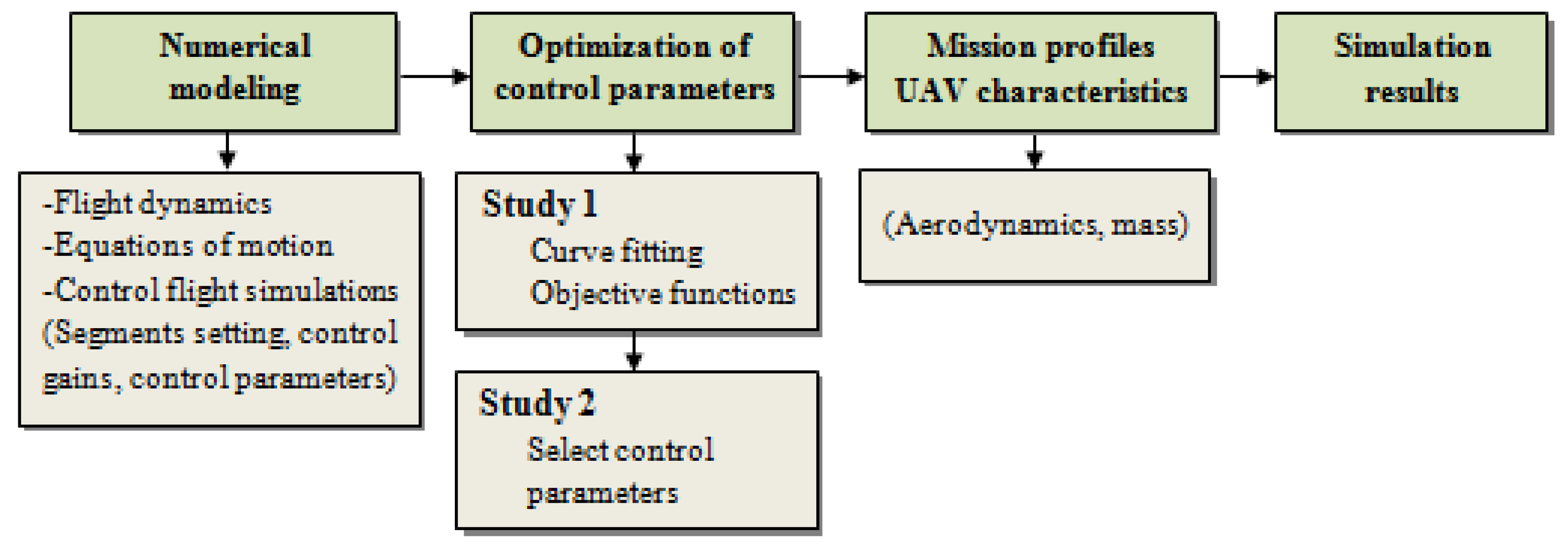
The remainder of this paper is structured as follows (Figure 1): Section 2 describes the numerical formulation encompassing the equations of motion, the control approach for various flight conditions, and the calculation of control gains from given control parameters. Section 3 details the procedure to identify the lower and upper bounds of the control parameters used in the parametric study aimed at selecting the control parameters’ combination for best performance. Section 4 presents the hybrid propulsion VTOL UAV characteristics and the different analyzed mission profiles. The results obtained from the simulations performed in the parametric study are discussed in Section 5. Section 6 contains the conclusions.

2. Numerical Modeling

2.1. Flight Dynamics

The aerodynamic and propulsion models, as well as the longitudinal equations of motion, are herein described since they are the tools for modeling the aircraft response to the environment and the control commands. Only the motion in the vertical xz-plane is represented here.

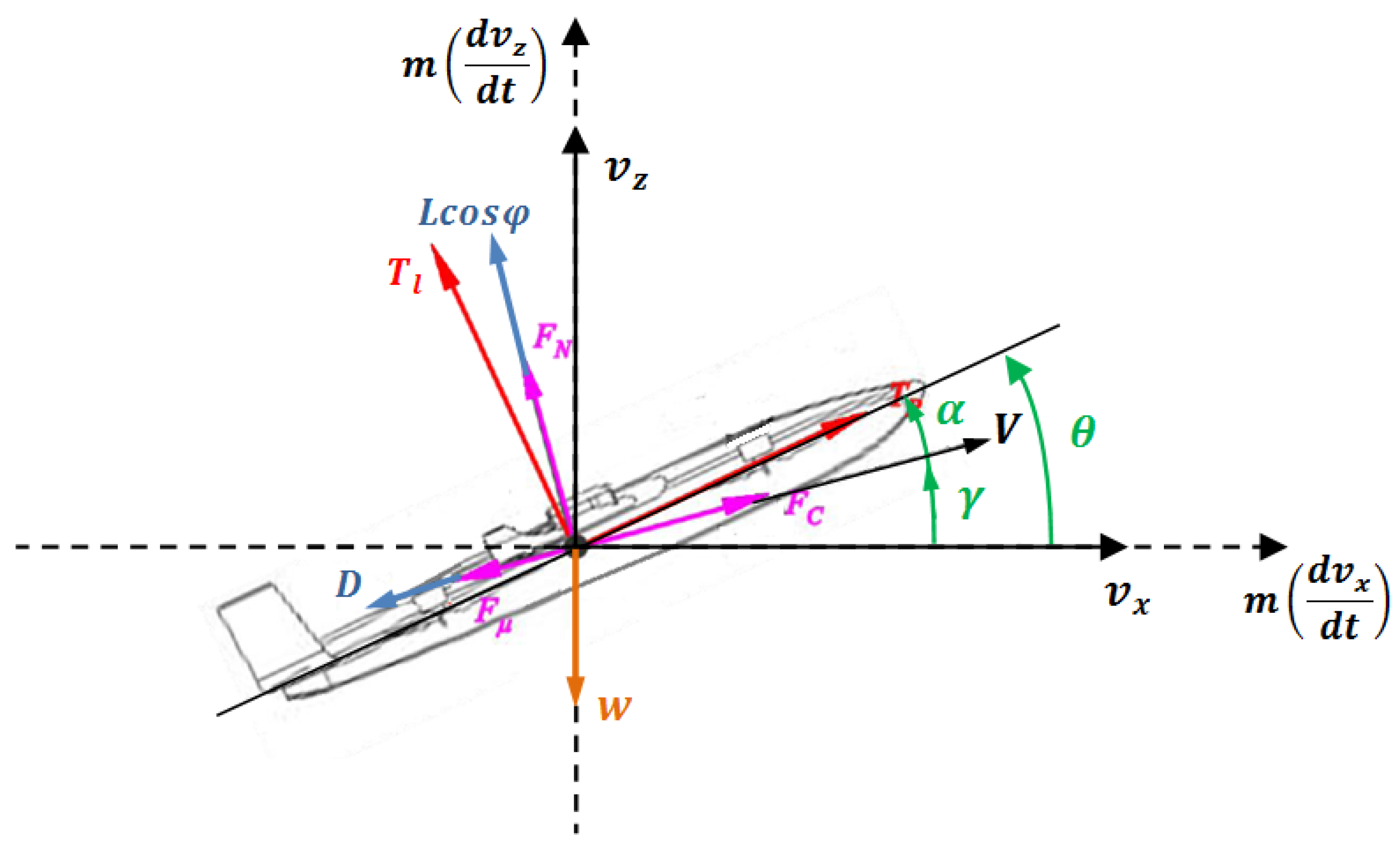
The acting forces on the UAV during a flight are shown in Figure 2, which include propulsive forces (in red), aerodynamic forces (in grey), ground forces (in pink), and weight (in orange), resulting from its motion through the air.

The flight airspeed V is given by:

$$V=\sqrt{v_x^2+v_z^2}$$

(1)

where $v_x$ and $v_z$ are the velocity component in x- and z- directions, horizontal and vertical, respectively.

The aircraft’s attitude angles are defined by the pitch angle $\theta$ and the bank angle $\phi$. The trajectory angle γ and the angle of attack α are related by:

$$\gamma =\mathrm{asin}\left(\frac{v_z}{V}\right)$$

(2)

$$\theta =\alpha +\gamma$$

(3)

In the presence of head wind ($v_w)$ in the x-direction, the flight speed is defined as:

$$V_a=\sqrt{{(v_x+v_w)}^2+v_z^2}$$

(4)

The angle of attack $\alpha$ becomes:

$$\alpha =\theta - \mathrm{asin}\left(\frac{v_z}{V_a}\right)$$

(5)

The resulting aerodynamic forces are defined as:

$$X_a=-Lcos\phi sin\gamma -Dcos\gamma$$

(6)

$$Z_a=Lcos\phi cos\gamma -Dsin\gamma$$

(7)

where $X_a$ and $Z_a$ represent the aerodynamic forces in the x- and z-directions, respectively, L is the aerodynamic lift force, and D the aerodynamic drag force.

The propulsive forces are composed of two components, the propulsion thrust $(T_p)$, and the lift thrust $(T_l)$. The propulsion thrust $(T_p)$ is parallel to the longitudinal axis of the aircraft, and the lift thrust $(T_l)$ is perpendicular to it. The resulting propulsive forces are:

$$X_p=T_{p}cos\theta -T_{l}cos\theta$$

(8)

$$Z_p=T_{p}sin\theta +T_{l}sin\theta$$

(9)

Ground forces consist of three components, which exist only when the aircraft is in contact with the ground. When the aircraft is launched by a catapult, there is the average force of the catapult ($F_c)$ and the ground reaction force ($F_n)$ that is normal to the trajectory, the latter being given by:

$$F_n=F_g\left(Wcos\gamma -L-T_{l}cos\alpha -T_{p}sin\alpha \right)$$

(10)

where $F_g$ is a factor that is 1 when the aircraft is in contact with the ground and 0 when it is airborne. $W$ is the aircraft weight.$F_{\mu }$ is the rolling friction forcewhich is given by:

$$F_{\mu }=\mu F_n$$

(11)

where $\mu$ is the rolling friction coefficient.

The resultant ground forces in the x- and z- directions are defined by:

$$X_g=-F_{n}sin\gamma +\left(F_c-F_{\mu }\right)cos\gamma$$

(12)

$$Z_g=F_{n}cos\gamma +\left(F_c-F_{\mu }\right)sin\gamma$$

(13)

The weight force components are just $X_w=0$ and $Z_w=W$.

2.2. Equations of Motion

Adding together all the components of the force described above and using Newton’s second law, the general equations of motion are:

$$m\frac{d{v}_x}{dt}=X_a+X_p+X_g+X_w$$

(14)

$$m\frac{d{v}_z}{dt}=Z_a+Z_p+Z_g+Z_w$$

(15)

2.3. Control during Flight Simulation

2.3.1. Setting Propulsion Thrust

During the forward flight, it is necessary to control the propulsion thrust to hold speed. By applying Newton’s second law, the force can be specified as a function of the speed error and is obtained as such:

$$X_{\gamma }=m\frac{dv}{dt}=k_{tv}\left(V_{ref}-V\right)$$

(16)

where $X_{\gamma }$ is the resultant of all the external forces acting on the system in the trajectory direction, m is the total mass, $k_{tv}$ is a gain constant to set propulsion thrust to hold speed, and $V_{ref}$ and V are the required and current speeds, respectively. The force in Equation (16) is also equal to:

$$X_{\gamma }=F_d+T_{p}cos\alpha$$

(17)

where $F_d=\left(X_a+X_g+X_w\right)cos\gamma +\left(Z_a+Z_g+Z_w\right)sin\gamma +T_{l}sin\alpha$ is the force in the trajectory direction, excluding the propulsion thrust component. By substituting Equation (17) into Equation (16), the required propulsion thrust is obtained as:

$$T_p=\frac{k_{tv}\left(V_{ref}-V\right)-F_d}{cos\alpha }$$

(18)

2.3.2. Setting Lift Thrust

During the vertical takeoff and vertical landing, it is necessary to achieve a given vertical speed. Thus, the lift thrust necessary to hold the rate of climb can be specified as a function of the rate of climb error in the following form:

$$Z=m\frac{d{v}_z}{dt}=k_{lv}\left(v_{z_{ref}}-v_z\right)$$

(19)

where $k_{lv}$ is a gain constant to control lift thrust to hold speed and $v_{z_{ref}}$ and $v_z$ are the required and current rates of climb, respectively. $Z$ is the resultant vertical force to calculate thrust to hold altitude and is defined by:

$$Z=F_{rc}+T_{l}cos\theta$$

(20)

where $F_{rc}$=$\left(Z_a+Z_g+Z_w\right)+T_{p}sin\theta$ is the sum of all vertical forces except for the lift thrust component.

From Equations (19) and (20), the required lift thrust is obtained as:

$$T_l=\frac{k_{lv}\left(v_{z_{ref}}-v_z\right)-F_{rc}}{cos\theta }$$

(21)

During the transition and hovering flight, it is necessary to maintain a given altitude. Then, the lift thrust necessary to hold the altitude can be given in the form:

$$Z=m\frac{d{v}_z}{dt}=m\frac{d^{2}z}{d{t}^2}=k_{t{h}_1}\left(z_{ref}-z\right)-k_{t{h}_2}\frac{dz}{dt}$$

(22)

where $z_{ref}$ is the required altitude, z is the current altitude and $k_{t{h}_1}$ and $k_{t{h}_2}$ are the proportional gain to set lift thrust to hold the altitude and its derivative, respectively.$Z$ is the resultant vertical force to calculate thrust to hold the altitude defined by Equation (20). From Equations (20) and (22), the required lift thrust to hold the altitude is obtained as:

$$T_l=\frac{k_{t{h}_1}\left(z_{ref}-z\right)-k_{t{h}_2}{v}_z-F_{rc}}{cos\theta }$$

(23)

2.3.3. Setting Pitch Angle

For hovering and vertical flight (vertical takeoff and vertical landing), it is necessary to hold position with a pitching attitude. The horizontal force can be written as:

$$X=m\frac{d{v}_x}{dt}=m\frac{d^{2}x}{d{t}^2}=k_{\gamma x_1}\left(x_{ref}-x\right)-k_{\gamma x_2}\frac{dx}{dt}$$

(24)

where $k_{\gamma x_1}$ denotes the proportional gain to control the pitch attitude to hold position, $k_{\gamma x_2}$ is the derivative gain to set the pitch attitude to hold position, and $x_{ref}$ and $x$ are the required position and the current position, respectively. $X$ represents the resultant horizontal force given by:

$$X=F_x+T_{l}sin\theta$$

(25)

where $F_x=\left(X_a+X_g+X_w\right)+T_{p}sin\theta$ denotesthe horizontal force, excluding the lift thrust component.

From Equations (24) and (25), the required pitch angle to hold position is obtained as:

$$\theta =asin\left[\frac{-k_{\gamma x_1}\left(x_{ref}-x\right)+k_{\gamma x_2}{v}_x+F_x}{T_l}\right]$$

(26)

During the conventional climb and descent phases, it is required to hold speed (V) by specifying a pitch angle (θ). The following equation can be used:

$$X_{\gamma v}=m\frac{dV}{dt}=k_{\gamma v}\left(V_{ref}-V\right)$$

(27)

where $k_{\gamma v}$ is a gain constant to hold speed with the pitch angle and $X_{\gamma v}$ is defined by:

$$X_{\gamma v}=F_t-Wsin\gamma$$

(28)

where $F_t=\left(X_p+X_g+X_a\right)cos\gamma +\left(Z_p+Z_g+Z_a\right)sin\gamma$ is the force in the trajectory direction, excluding the weight component. Substituting Equation (28) in Equation (27) and using Equation (3), the required pitch angle to hold speed is obtained as:

$$\theta =asin\left[\frac{k_{tv}\left(V_{ref}-V\right)-F_t}{W}\right]+\alpha$$

(29)

For the transition and cruise, holding the altitude (z) by specifying the pitch angle ($\theta )$ can be achieved by writing the rate of climb as follows:

$$\frac{dz}{dt}=Vsin\gamma =k_{\gamma z}\left(z_{ref}-z\right)$$

(30)

where $k_{\gamma z}$ is the gain constant to hold the altitude with the pitch angle. Then, using Equation (3), the required pitch angle to hold the altitude is obtained as:

$$\theta =asin\left[\frac{k_{\gamma z}\left(z_{ref}-z\right)}{V}\right]+\alpha$$

(31)

2.3.4. Control Gains and Control Parameters

The gains’ values used to set the required pitch angle, propulsion thrust, or lift thrust are obtained from the solution of the control of differential equations.

Equations (16), (19), (27), and (30) are first-order differential equations of the form

$$\frac{du}{dt}+\frac{k}{c}u=\frac{\mathrm{k}}{c}{u}_{ref}$$

(32)

where u is the controlled variable, $u_{ref}$ is the required value of the controlled variable, k is the control gain, and c is a characteristic of the system. The solution of Equation (32) is given by:

$$u=u_{ref}+C{e}^{\frac{-k}{c}\mathrm{t}}$$

(33)

where C is the amplitude. Considering that one requires half amplitude to be achieved at the time $t=t_u$, the control gain k becomes:

$$k=-\frac{c}{t_u}\ln \left(\frac{1}{2}\right)$$

(34)

In Equation (34), c takes the value of m from Equations (16), (19), and (27) or the unit value from Equation (27). Here $t_u$ is the time constant which is a specified control parameter.

Equations (22) and (24) are second-order differential equations of the form

$$\frac{d^{2}u}{d{t}^2}+\frac{k_2}{c}\frac{du}{dt}+\frac{k_1}{c}u=\frac{k_1}{c}{u}_{ref}$$

(35)

where $k_1$ and $k_2$ are the proportional and the derivative control gains, respectively, and whose solution is given by

$$\left\{\begin{array}{c}{k}_1=c\frac{{\omega }^2}{1-{\eta }^2}, with \omega =\frac{2\pi }{T}\\ k_2=2c\eta \frac{\omega }{\sqrt{1-{\eta }^2}},with 0<\eta <1 \end{array}\right.$$

(36)

where $\omega$ is the frequency, $\eta$ is the damping ratio, and T the period. These two latter parameters are also specified control parameters. In Equation (36), c takes the value of m from Equations (22) and (24).

From the above equations, the gains are obtained given the control parameters. These are as follows: $k_{tv}$ is set as a function of the time constant $t_{tv}$; $k_{lv}$ as a function of the time constant $t_{lv}$; $k_{t{h}_1}$ and $k_{t{h}_2}$ are set as functions of damping ratio ${\eta }_{th}$ and period $T_{th}$; $k_{\gamma x_1}$ and $k_{\gamma x_2}$ are set as functions of damping ratio ${\eta }_{\gamma }$ and period $T_{\gamma }$; $k_{\gamma v}$ is set as a function of the time constant $t_{\gamma v}$, and $k_{\gamma z}$ is set as a function of the time constant $t_{\gamma z}$.

3. Optimization of Control Parameters

Two objectives are considered in the current study. One is to identify the control parameters and corresponding lower and upper bounds such that a given mission is well simulated without control divergence. The other is to analyze their effects on the UAV flight simulation by performing both conventional and VTOL segments in different mission profiles in order to obtain the best combination of control parameters that minimize a given mission performance function.

In the first objective, the mission segments that exhibit transient oscillatory responses are analyzed. As the optimal solution cannot be found from an arbitrary initial choice, one way to accurately determine the period of oscillation and the damping ratio of the motion is to find the best-fit curve through the simulation data points. To this end, the least-squares polynomial-curve fit is used for the pitch attitude and thrust responses. Hence, all peaks and valleys of the oscillatory response are detected automatically and used to obtain the maximum and minimum bound curves of the motion; then, a sinusoidal-fit curve equation is used to fit the data points and to obtain the amplitude, the damping, the frequency, and the phase angle, as follows:

$$\mathsf{\Psi }\left(t\right)=A{e}^{-\eta {\omega }_{n}t}cos\left({\omega }_n\sqrt{1-{\eta }^2}t+\beta \right)$$

(37)

where $A$, $\eta$, ${\omega }_n$, and $\beta$ represent the amplitude, the damping ratio, the natural frequency, and the phase angle, respectively.

This procedure is applied to the cruise segments, which exhibit the transient oscillatory response at the end of the transition to gain speed or at the end of a climb. After extracting the values of $A$, $\eta$, ${\omega }_n$, and $\beta$, we need to define the lower and upper bounds of the control parameters. This is performed by separately analyzing the thrust and the pitch angle (θ) curves of each of the specified mission profiles. The function in this problem, Equation (38), is calculated for every ith case in a set of n control parameter combinations:

$$f_{parm,i}=W_A\frac{A_i}{A_{avr}}+W_{\eta }\frac{{\eta }_i}{{\eta }_{avr}}+W_{\omega }{\left(\frac{{\omega }_{n,i}}{{\omega }_n{}_{avr}}\right)}^{-1}$$

(38)

where $W_A$,$W_{\eta }$, and $W_{\omega }$ are weighting coefficients; $A$ and $A_{avr}$ represent the amplitude and the average amplitude, respectively; $\eta$ and ${\eta }_{avr}$ are the damping ratio and the average damping ratio, respectively; ${\omega }_n$ and ${\omega }_n{}_{avr}$ are the natural frequency and the average natural frequency, respectively. The value of $f_{parm}$ must be maximized to reduce the oscillations and smooth out the control response. From all analyzed mission profiles, the minimum and maximum values of the control parameters that maximize Equation (38) are selected as lower and upper bounds for the next analysis.

The second objective is to optimize the control parameters by selecting the best combination that minimizes the following equation:

$$f_{obj,i}=W_1\frac{t_i}{t_{max}}+W_2\frac{x_i}{x_{max}}-W_3\frac{m_{fuel,i}}{m_{fue{l}_{max}}}-W_4\frac{E_{batt,i}}{E_{bat{t}_{max}}}$$

(39)

where $W_1$,$W_2$,$W_3$, and $W_4$ denote weighting coefficients; $t$ and $t_{max}$ are the time and the maximum time at the end of the mission, respectively; $x$ and $x_{max}$ are the hover x-position difference and the maximum hover x-position difference, respectively; $m_{fuel}$ and $m_{fue{l}_{max}}$ are the remaining fuel mass and the maximum remaining fuel mass at the end of the mission, respectively; $E_{batt}$ and $E_{bat{t}_{max}}$ are the remaining battery energy and the maximum remaining battery energy at the end of the mission, respectively.

Equation (39) is calculated for every ith specified combination of the control parameters. The minimization of $f_{obj}$ aims to achieve better control performance by selecting an appropriate combination of the control parameters weighing the resulting mission time, x distance difference, and fuel mass and battery energy consumption. This approach results in selecting the control parameter combination that leads to a mission that takes less time to complete and uses less energy.

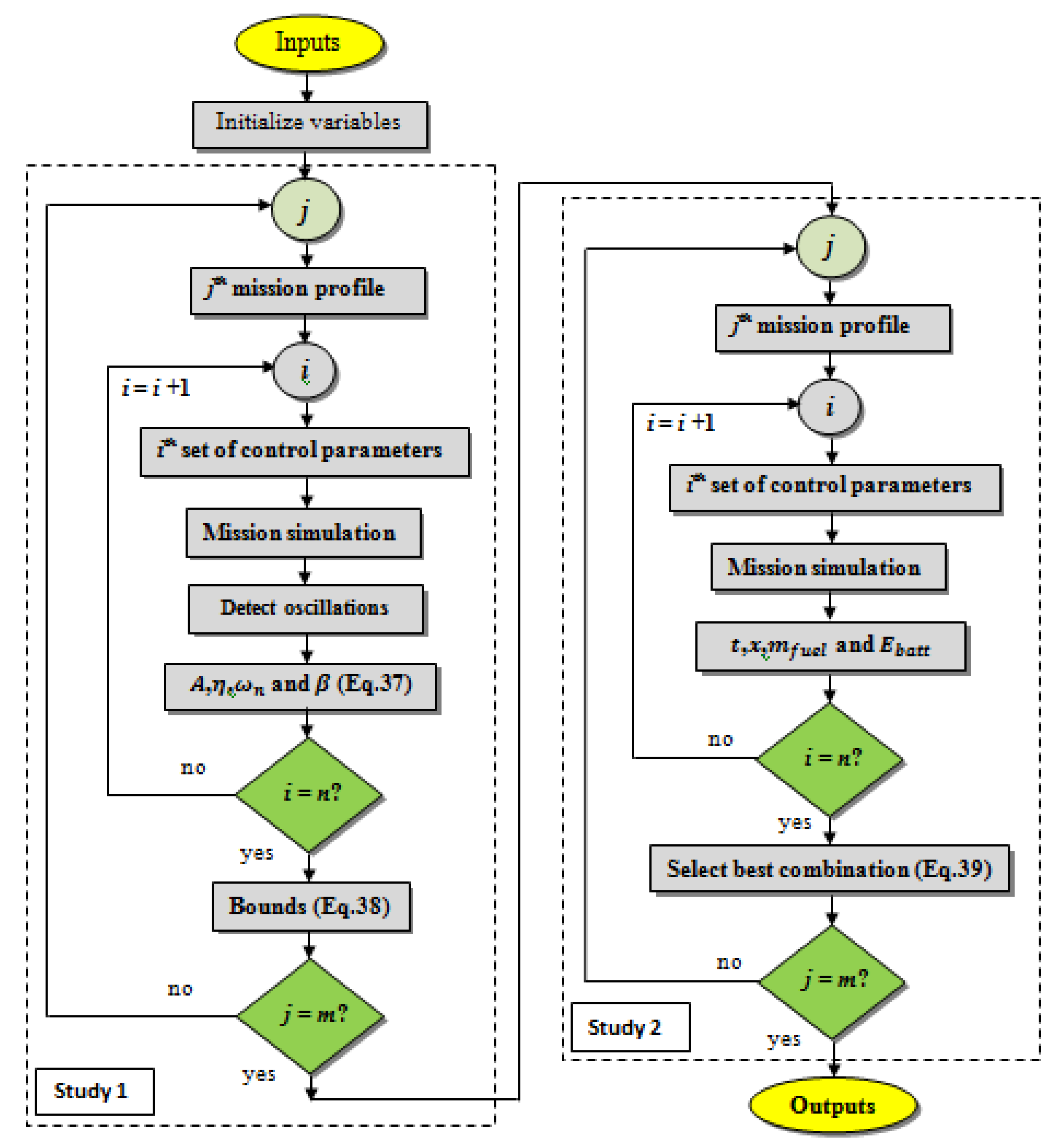
The procedure to estimate the best control parameters is presented in the flow chart shown in Figure 3. In the first study, the curve fitting procedure is applied to define the minimum and maximum bound curves, using Equation (37) to fit the flight simulation data points and to obtain the amplitude, damping, frequency, and phase angle of the transient motion. Then, a set of minimum, maximum, and step-change values for every control parameter is applied in a set of n combinations. After running the possible combinations affecting the cruise, the control parameters’ values that minimize Equation (38) are selected as bounds for the second study. Then, in the second study, the control parameters are optimized by minimizing Equation (39) to achieve better control performance.

4. Mission Profiles and UAV Characteristics

In this study, six different UAV sample mission profiles are analyzed. The selected different profiles capture the different flight capabilities typical of a fixed-wing multi-rotor VTOL aircraft. The first mission profile (Mission 1) consists of nine flight phases, starting with a vertical takeoff at 3 m/s up to 45 m altitude, an acceleration transition up to 20 m/s, a cruise of 200 m at 23 m/s, a deceleration transition to 0 m/s, a hover of 60 s at 45 m altitude, a second acceleration transition, a cruise of 200 m at 23 m/s and another deceleration to 0 m/s, and finally a vertical landing to 0 m altitude at −1.5 m/s.

In the second mission profile (Mission 2), five flight phases are chosen: a vertical takeoff at 3 m/s up to 45 m altitude, an acceleration transition up to 20 m/s, a cruise of 2000 m at 23 m/s, and a deceleration transition to 0 m/s before a vertical landing to 0 m altitude at −1.5 m/s.

Eleven flight phases are used in the third mission profile (Mission 3): a vertical takeoff at 3 m/s up to 45 m altitude, an acceleration transition up to 23 m/s, a climb at 23 m/s till 100 m altitude before a cruise of 200 m at 100 m altitude at the same speed, a deceleration transition, a hover of 60 s at 100 m altitude, a second acceleration transition, a cruise of 200 m distance at 23 m/s and 100 m altitude, a descent at 28 m/s to achieve 45 m altitude and another deceleration to 0 m/s, and at the end a vertical landing to 0 m altitude at −1.5 m/s.

For the fourth mission profile (Mission 4), seven phases are studied: a vertical takeoff at 3 m/s up to 45 m altitude, an acceleration transition up to 23 m/s, a climb of 100 m at 23 m/s till 100 m altitude before a cruise of 2000 m at 100 m altitude at the same speed, a descent at 28 m/s and 45 m altitude, a deceleration transition, and a vertical landing to 0 m altitude at −1.5 m/s.

Mission profile five (Mission 5) consists of a takeoff, a climb of 100 m at 23 m/s, a cruise of 200 m at 23 m/s, a transition, a hover of 60 s at 100 m altitude, a transition and a second cruise of 200 m distance and 100 m altitude at 23 m/s, and a final descent at 28 m/s to the takeoff altitude with the goal of landing.

The last mission profile (Mission 6) has five flight phases: a takeoff at 23 m/s, a climb of 100 m at 23 m/s, and a cruise of 2000 m at 23 m/s, ending by descent at 28 m/s to the takeoff altitude with the goal of landing.

The studied hybrid propulsion VTOL UAV is typical of a light UAV under 25 kg of the maximum takeoff mass. It has one internal combustion engine for horizontal thrust and eight electric motors arranged in pairs in a quadcopter configuration for the vertical lift. The UAV’s main characteristics are presented in

Table 1. UAV characteristics.

Aircraft Mass [kg]	Fuel Mass [kg]	Wing Area [m2]	${\mathit{C}}_{{\mathit{L}}_{\mathit{m}\mathit{a}\mathit{x}}}$
24.87	1.13	0.910	1.32

. The model combines numerous system components: an internal combustion engine (ICE) coupled with a generator and propeller for horizontal propulsion, whereas vertical propulsion comprises a battery, electric motors (EM), an electric speed controller (ESC), and propellers. The aerodynamic and propulsion characteristics of the UAV were estimated using the methodology presented by Albuquerque et al. [24] and are summarized below in Equations (40)–(42).

The lift and drag coefficients, $C_L$ and $C_D$, respectively, can be defined by the following equations:

$$\left\{\begin{array}{c}{C}_L=0.427+0.0918\alpha \\ C_D=0.0295-0.0027C_L+0.0301C_L{}^2\end{array}\right.$$

(40)

Given the UAV characteristics and mission data, the propulsion system curves of the internal combustion engine and propeller used to estimate the forward flight thrust are:

$$\left\{\begin{array}{c}{V}_{max}=12.27+178.49{\delta }_{eng}-262.6{\delta }_{eng}{}^2+246.81{\delta }_{eng}{}^3-90.12{\delta }_{eng}{}^4\\ N_{max}=2046+29768{\delta }_{eng}-43799{\delta }_{eng}{}^2+41168{\delta }_{eng}{}^3-15031{\delta }_{eng}{}^4\\ N=N_{max}\exp (-0.63-0.447f_v+2.518f_v{}^2-1.705f_v{}^3+0.261f_v{}^4)\\ T_p={\delta }_{eng}\left(\frac{\rho }{{\rho }_0}\right)\ln \left(N\right)\left(11.07-10.02f_v-13.49f_v{}^2+33.1f_v{}^3-20.73f_v{}^4\right)n_{eng}\end{array}\right.$$

(41)

where $V_{max}$ is the maximum airspeed of the propeller, ${\delta }_{eng}$ is the internal combustion engine power setting, $N_{max}$ is the maximum engine speed, N is the current engine speed, $f_v=V/V_{max}$, ρ is the air density, ${\rho }_0$ is the ISA sea-level air density, and $n_{eng}$ is the number of engines.

The propulsion system curves of the electric motors and propellers used to estimate the vertical flight thrust are defined as follows:

$$\left\{\begin{array}{c}{V}_{max}=0.31+21.64{\delta }_{mot}+9.79{\delta }_{mot}{}^2-15.27{\delta }_{mot}{}^3+6.86{\delta }_{mot}{}^4\\ I={\delta }_{mot}{}^{1.75}{\left(\frac{\rho }{{\rho }_0}\right)}^{0.5}\left(96.84-20.53f_v+118.73f_v{}^2-362.86f_v{}^3+207.2f_v{}^4\right)\\ T_l={\delta }_{mot}\left(\frac{\rho }{{\rho }_0}\right)I^{0.56}\left(11.42-18.19f_v+28.42f_v{}^2-34.48f_v{}^3+12.96f_v{}^4\right)n_{mot}\end{array}\right.$$

(42)

where ${\delta }_{mot}$ is the electrical motors power setting, I is the motor’s drawn current, and $n_{mot}$ is the number of electric motors.

5. Results and Discussion

A parametric study is carried out to analyze the effects of the control parameters on the UAV flight simulation using conventional and VTOL flight segments in different mission profiles.

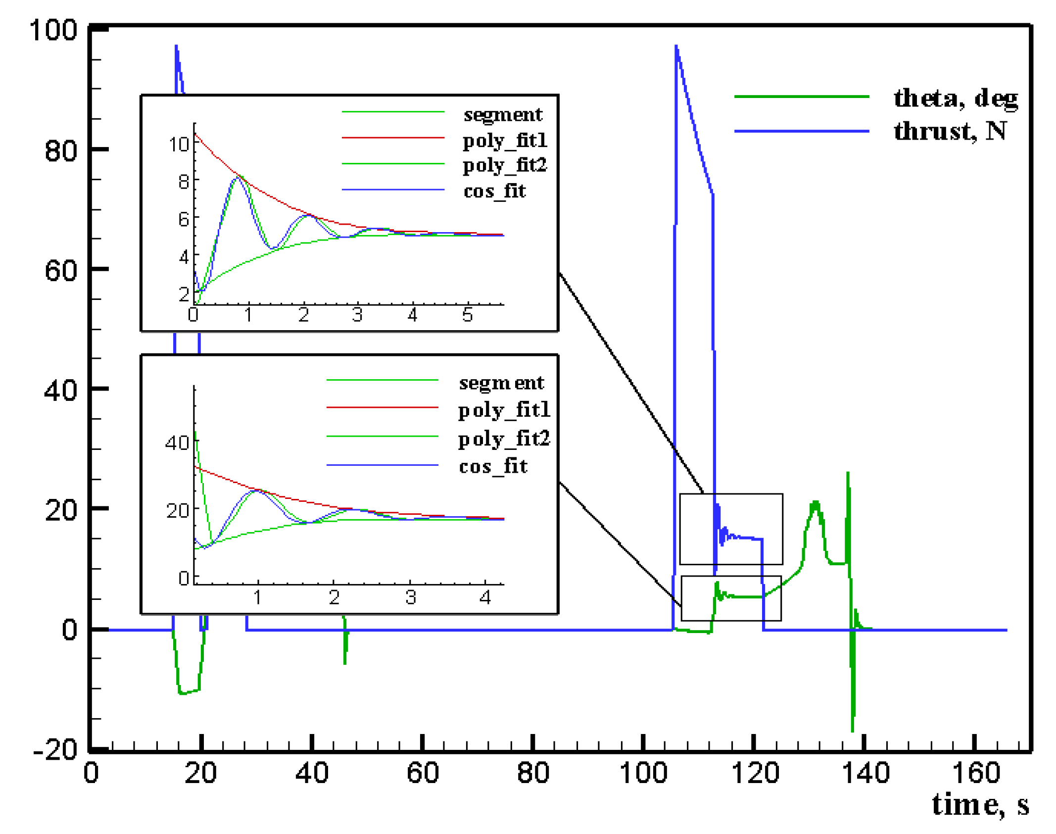
Figure 4 shows the polynomial-curve fit results of the pitch angle (θ) and the propulsion thrust responses for the cruise ofMission1. From these, all the peaks and valleys are detected automatically and used in the curve fitting procedure to define the maximum and minimum bound curves using Equation (37) to fit the flight simulation data points to obtain the amplitude, damping, frequency, and phase angle. A set of minimum, maximum, and step-change values for every control parameter was defined, and after running the possible combinations affecting the cruise, the control parameters’ values that minimize Equation (38) were selected as bounds and are shown in

Table 2. Control parameter bounds obtained from analysis 1.

Control Parameters	Mission 1	Mission 2	Mission 3	Mission 4	Mission 5	Mission 6
$t_{\gamma v}$ [s]	15.00–25.00	15.00–25.00	15.00–25.00	15.00–25.00	15.00–25.00	15.00–25.00
$t_{\gamma h}$ [s]	1.50–2.17	1.50–2.17	1.50–2.17	1.50–2.17	1.50–2.17	1.50–2.17
$t_{tv}$ [s]	11.17–25.00	11.17–25.00	10.00–25.00	10.00–25.00	10.00–25.00	10.00–25.00
$t_{lv}$ [s]	0.15–0.25	0.15–0.25	0.15–0.25	0.15–0.25	0.15–0.25	0.15–0.25
$T_{th}$ [s]	2.00–6.00	2.00–6.00	4.67–6.00	4.67–6.00	4.67–6.00	4.67–6.00
${\eta }_{th}$ [–]	0.52–0.60	0.52–0.60	0.37–0.60	0.37–0.60	0.37–0.48	0.37–0.48
$T_{\gamma }$ [s]	2.50–6.00	2.50–6.00	2.50–6.00	2.50–6.00	2.50–6.00	2.50–6.00
${\eta }_{\gamma }$ [–]	0.20–0.60	0.20–0.60	0.20–0.60	0.20–0.60	0.20–0.60	0.20–0.60

.

Then, a second parametric study is carried out to optimize the control parameters by minimizing Equation (39) to achieve better control performance by selecting an appropriate combination of the control parameters, taking into account the time, x-distance difference, fuel mass, and battery energy consumption. The optimized parameters are shown in

Table 3. Control parameter inputs obtained from analysis 2.

Control Parameters	Mission 1	Mission 2	Mission 3	Mission 4	Mission 5	Mission 6	AVR	STDEV
$t_{\gamma v}$ [s]	15	15	15	18.33	15	15	15.56	1.36
$t_{\gamma h}$ [s]	1.94	1.72	1.5	1.5	1.5	2.17	1.72	0.28
$t_{tv}$ [s]	15.78	20.56	15	10	10	25	16.06	5.91
$t_{lv}$ [s]	0.15	0.18	0.15	0.15	0.15	0.15	0.16	0.01
$T_{th}$ [s]	6.0	6.0	6.0	6.0	6.0	4.67	5.78	0.54
${\eta }_{th}$ [–]	0.53	0.58	0.37	0.37	0.37	0.37	0.43	0.1
$T_{\gamma }$ [s]	6.0	6.0	6.0	6.0	6.0	6.0	6.0	0
${\eta }_{\gamma }$ [–]	0.2	0.2	0.2	0.2	0.2	0.2	0.2	0

for each mission with the average values (AVR) and the standard deviation (STDEV).

The simulation results are shown in Figure 5, Figure 6, Figure 7, Figure 8, Figure 9 and Figure 10, where the traveled distance, altitude, pitch angle, and propulsion thrust are plotted as functions of time.

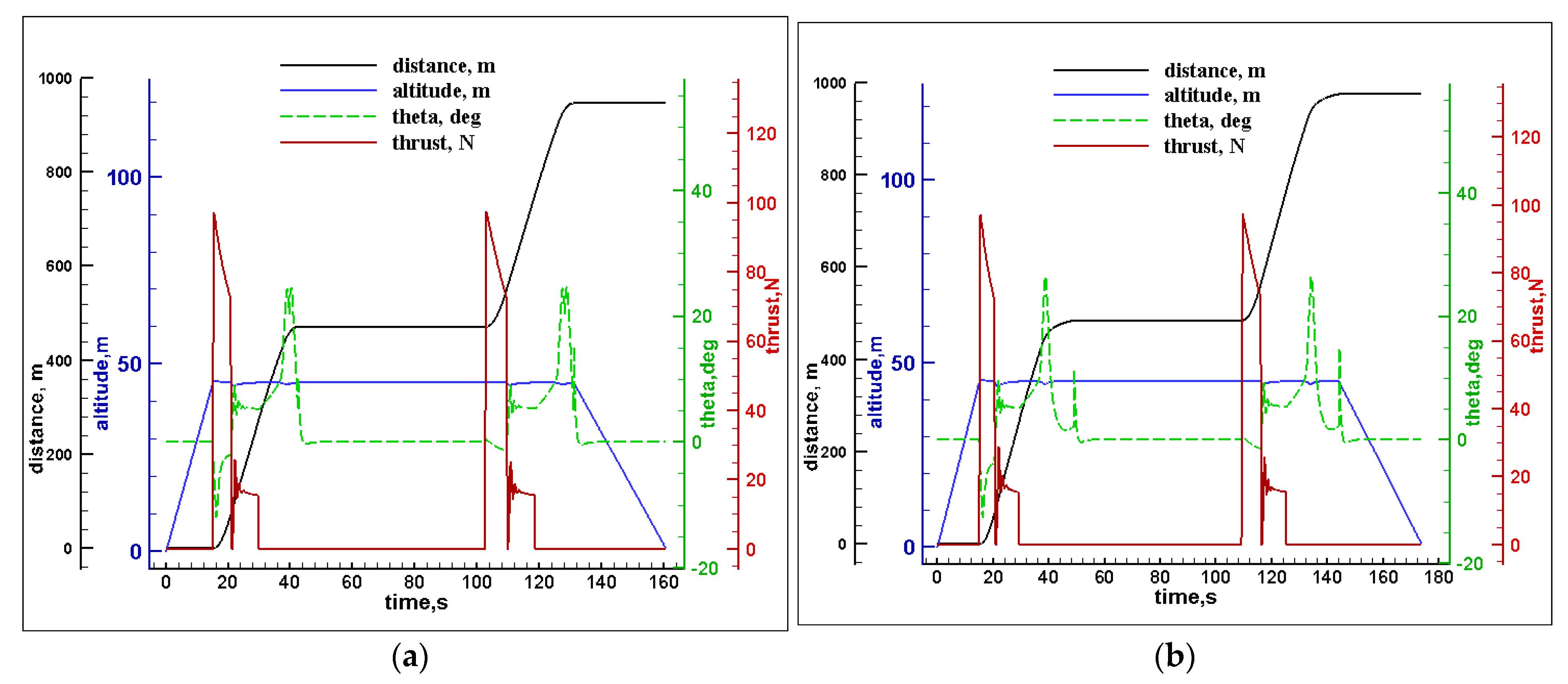
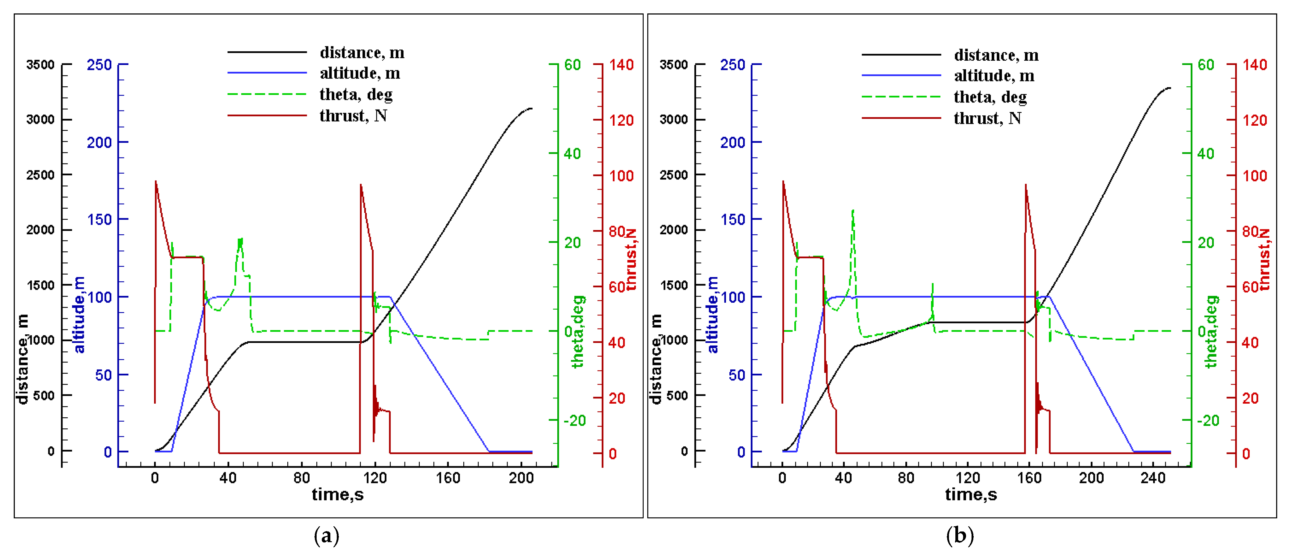
In Figure 5a, during the vertical takeoff from t = 0 s to 15 s, the UAV climbs vertically until 45 m of altitude is reached under the electric rotors thrust where the pitch angle is kept at 0°, then it starts to move forward for the acceleration transition with the engine thrust while being assisted by the electric motors until the speed of 20 m/s is achieved, with a pitch angle of −10°. After t = 20.7 s, the electric motors are turned off, and the UAV starts cruising for 200 m at 23 m/s using the engine thrust, where lift force is obtained from the wings. At t = 29.8 s, the UAV switches to the electric motors and turns off the engine; the pitch angle increases up to 25°, creating an increased drag force for the deceleration transition until the speed reaches 0 m/s. Then, it hovers for 60 s, and the pitch angle becomes 0° again. At t = 102 s, the UAV starts the engine for the acceleration transition while the rotational speed of the motor decreases until the speed reaches 20 m/s, then the electric motors are turned off for the cruise at 23 m/s for 200 m using only the engine thrust, where lift force is obtained entirely from the wings; another deceleration transition starts at t = 118 s, where the engine is turned off, and the electric motors are turned on; the pitch angle rises to increase the drag force until the speed becomes 0 m/s, and the UAV starts the vertical landing at t = 131.1 s using electric motors, and the pitch angle becomes 0° again. From Figure 5b, we can see that between t = 29.2 s and t = 48 s, the UAV took 7 s longer to start the hover than in Figure 5a. This is also noticed during the second transition from t = 125 s to 144 s.

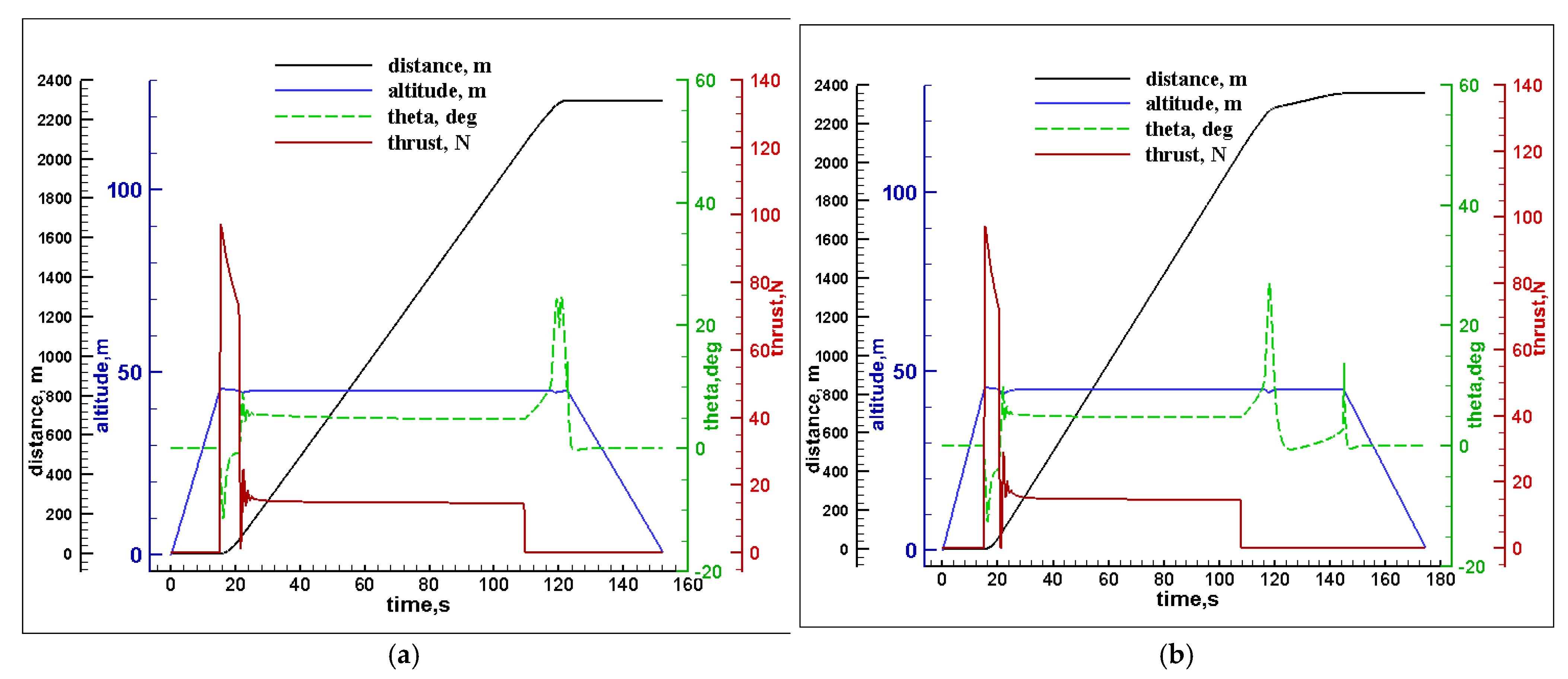
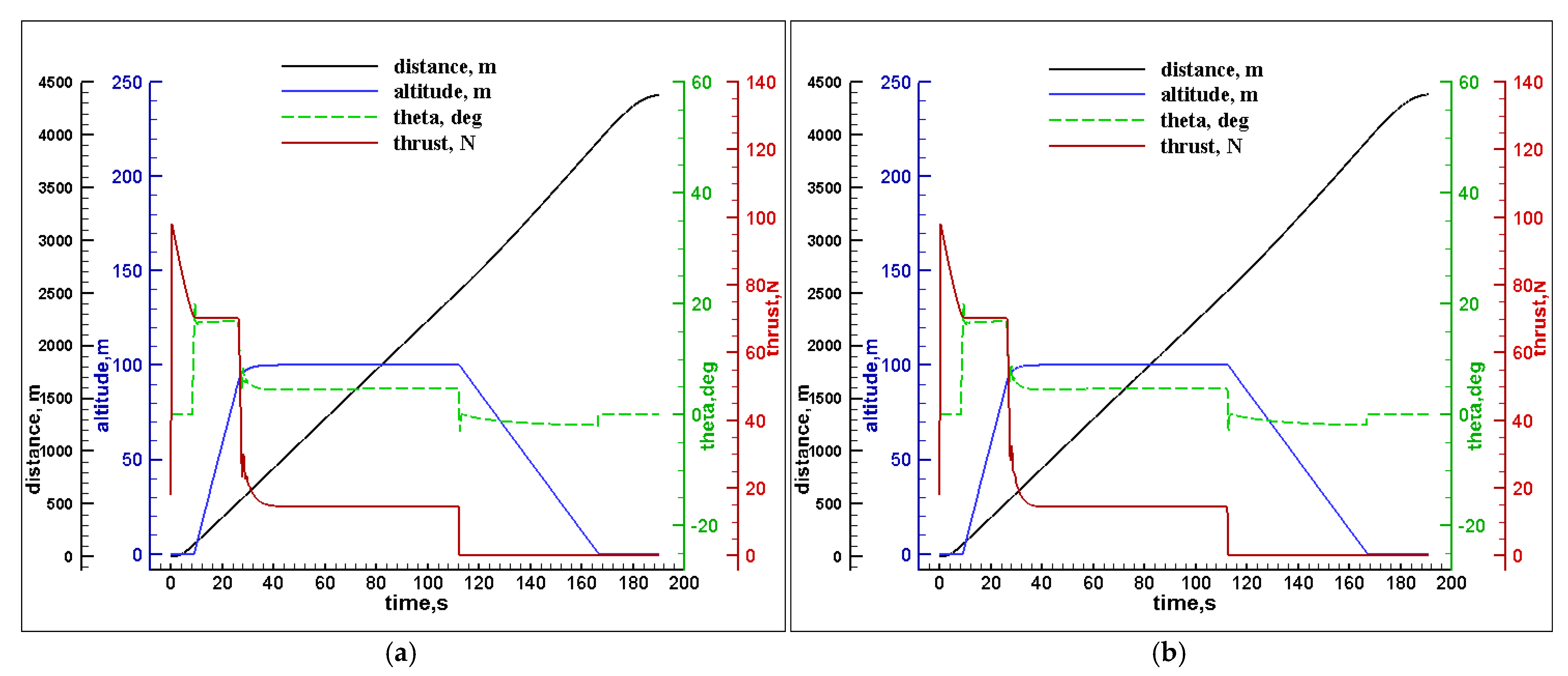
In Figure 6a, the UAV climbs vertically and reaches 45 m of altitude under the electric motors, where the pitch angle is kept at 0° for 15 s; then it starts to move forward for the acceleration transition with the engine thrust while being assisted by the electric motors until the speed of 20 m/s is achieved, in which the pitch angle becomes −10° due to the propulsion engine. After 21.2 s, the electric motors are turned off, and the UAV starts cruising using the engine thrust, and the lift force is obtained from the wings for 2000 m at 23 m/s. At t = 109.3 s, the UAV switches to the electric motors and turns off the engine, and the pitch angle increases to 25°, leading to an increased drag force for the deceleration transition until the speed reaches 0 m/s. At t = 122.6 s, the pitch angle becomes 0° again, and the UAV starts the vertical landing. Figure 6b shows the mission profile with the average parameters in which the UAV spends almost three times longer than when using the optimized parameters to switch from the cruise to the vertical landing between 107.7 s and 144.7 s.

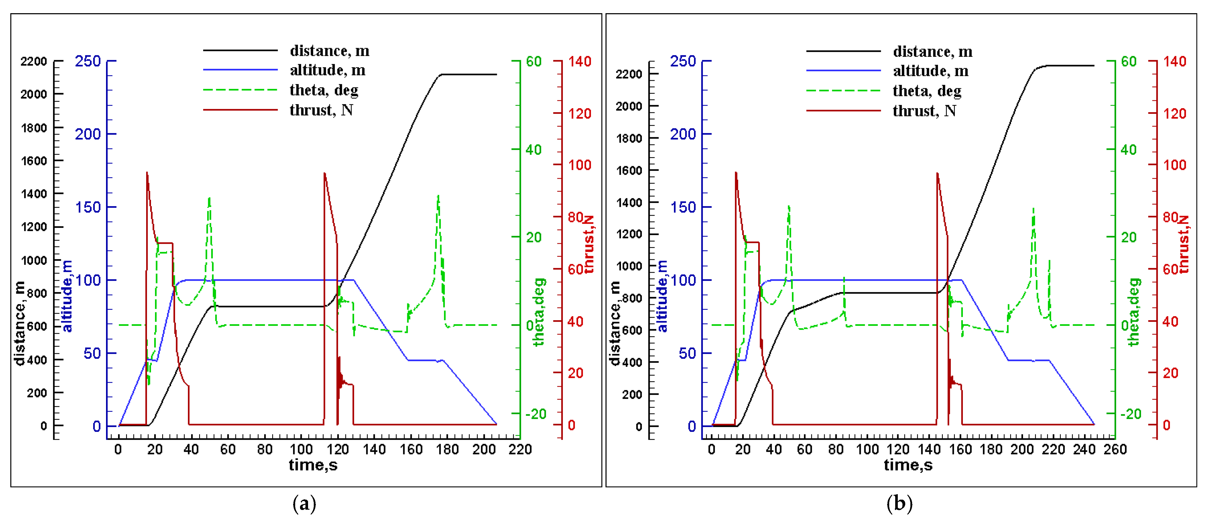
In Figure 7a, from t = 0 s to t = 15 s, the UAV starts the vertical takeoff to reach 45 m of altitude using the electric motors and a pitch angle of 0°; then the engine thrust is turned on to get the horizontal speed while the rotational speed of the electric motor decreases. At t = 19.9 s, the horizontal speed reaches 23 m/s, the UAV starts to climb as a conventional fixed-wing aircraft to reach 100 m altitude, and the electric motors are turned off. At t = 29.7 s, the UAV starts cruising for 200 m using the engine thrust, where the lift force is obtained from the wings. From t = 38.3 s to 52.2 s, the engine is turned off, and the electric motors are turned on for the deceleration transition, making the pitch angle become 25°, causing an increased drag force until the speed achieves 0 m/s to hover for 60 s using the electric motors. At t = 112.4 s, the UAV switches to an acceleration transition, where the engine is turned on while the rotational speed of the electric motor decreases; at t = 119.4 s, the horizontal speed reaches 23 m/s, and the UAV starts cruising for 200 m using only the engine thrust while the electric motors are turned off, where lift force is obtained entirely from the wings. At t = 128.4 s, the UAV starts descending to reach 45 m of altitude until t = 158 s, where the UAV switches to the electric motors and turns off the engine, and the pitch angle is increased, leading to an increase in drag force for the deceleration transition until the speed reaches 0 m/s. Here, the pitch angle becomes 0° again, and the UAV starts the vertical landing using the electric motors. The effect of the average parameters can be seen in Figure 7b, in which delays of 32 s and 8 s are observed relative to the optimized parameters’ case during the deceleration transitions, the first between t = 38.7 s and t = 85 s and the second between t = 19.3 s and 217 s, respectively.

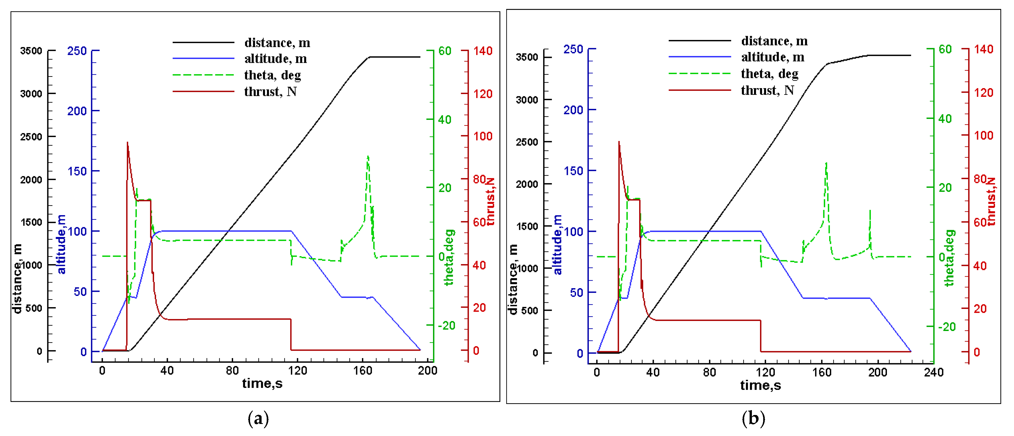
Figure 8a shows the results of Mission 4, where the UAV starts with a vertical takeoff to 45 m of altitude using the electric motors and a pitch angle of 0° until t = 15 s; then the engine thrust is turned on to get the horizontal speed, while the rotational speed of the electric motors decreases for the acceleration transition. At t = 20.8 s, the horizontal speed reaches 23 m/s, and the UAV climbs until an altitude of 100 m is reached as a conventional fixed-wing aircraft with the electric motors turned off. At t = 30.5 s, the UAV starts cruising for 2000 m using the engine thrust, where the lift force is obtained from the wings. At t = 116.9 s, the UAV starts descending to reach an altitude of 45 m until t = 146.5 s, where the UAV switches to the electric motors and turns off the engine. In the process, the pitch angle increases, leading to a greater drag force for the deceleration transition until the speed reaches 0 m/s. At t = 166.8 s, the pitch angle becomes 0° again, and the UAV lands vertically using the electric motors. In Figure 8b, we can also notice that the UAV takes 27 s longer in the deceleration transition from t = 146 s when compared to Figure 8b.

Figure 9a presents the results of Mission 5. The UAV starts with a conventional takeoff using the engine; at t = 8.3 s, the horizontal speed reaches 23 m/s, and the UAV climbs as a conventional fixed-wing aircraft up to an altitude of 100 m. After t = 26 s, the UAV starts cruising for 200 m. From t = 34.9 s to 51.6 s, the engine is turned off, and the electric motors are turned on in the deceleration the transition, where the pitch angle increases, causing an increased drag force until the speed achieves 0 m/s to hover for 60 s using the electric motors. At t = 111.8 s, the UAV switches to the acceleration transition, in which the engine is turned on, while the rotational speed of the electric motors decreases; at t = 118.9 s, the horizontal speed reaches 23 m/s, and the UAV starts cruising for 200 m using only the engine thrust, while the electric motors are turned off until t = 129.7 s when the UAV starts descending to the final landing. Looking at Figure 9b, from t = 34.8 s, the UAV takes 70 s in the deceleration transition before starting hovering, which is 45 s longer than when using the optimized parameters (Figure 9a).

Figure 10a shows the results of Mission 6. The UAV starts with a conventional takeoff using the engine, and at t = 8.3 s, the horizontal speed reaches 23 m/s when the UAV climbs as a conventional fixed-wing aircraft up to an altitude of 100 m. After t = 26 s, the UAV starts cruising for 2000 m. From t = 34.9 s to 51.6 s, the engine is turned off, and the electric motors are turned on in the deceleration transition, where the pitch angle is increased, causing the drag force to increase until the speed achieves 0 m/s to hover for 60 s using the electric motors. From t = 111.8 s, the UAV switches to an acceleration transition, in which the engine is turned on while the rotational speed of the electric motors decreases; at t = 118.8 s, the horizontal speed reaches 23 m/s, and the UAV starts cruising for 2000 m using only the engine thrust, while the electric motors are turned off. When t = 127.9 s, the UAV starts descending until the final landing. Compared with Figure 10b, no differences can be seen in this mission profile since there was no transition segment.

From the comparison of the results between the mission simulations using the optimized and the average control parameters, we can notice that the control parameters affect the mission in each deceleration transition, resulting in a longer time to reduce the cruise speed to stand still. This segment is characterized by a large increase in pitch angle to increase the drag to help reduce the speed in a short time. It is observed that if the control parameters in this segment are not well-tuned, the controller struggles to adjust the pitch angle.

Table 4. Comparison of the results for Mission 1.

	Optimized Parameters				Average Parameters
Flight	Δt [s]	Δx [m]	$\mathbf{\Delta }{\mathit{m}}_{\mathit{f}\mathit{u}\mathit{e}\mathit{l}} \left[\mathbf{k}\mathbf{g}\right]$	$\mathbf{\Delta }{\mathit{E}}_{\mathit{b}\mathit{a}\mathit{t}\mathit{t}} \left[\mathbf{k}\mathbf{J}\right]$	Δt [s]	Δx [m]	$\mathbf{\Delta }{\mathit{m}}_{\mathit{f}\mathit{u}\mathit{e}\mathit{l}} \left[\mathbf{k}\mathbf{g}\right]$	$\mathbf{\Delta }{\mathit{E}}_{\mathit{b}\mathit{a}\mathit{t}\mathit{t}} \left[\mathbf{k}\mathbf{J}\right]$
V-takeoff	14.9	0	0	49.713	14.9	0	0	49.698
Transition	5.8	66.245	0.001	12.332	5.4	60.301	0.001	13.334
Cruise	9	201.294	0.001	0.168	8.9	200.221	0.001	0.239
Transition	12.7	203.044	0.001	9.729	19.7	223.558	0.001	23.069
Hover	60.1	0	0.001	122.972	60.1	0	0.001	122.976
Transition	6.9	74.569	0.001	12.427	6.9	74.493	0.001	12.444
Cruise	9.1	202.174	0.001	0.141	9.1	202.135	0.001	0.143
Transition	12.5	198.42	0.001	9.733	19	213.926	0.001	22.45
V-landing	29.6	0	0	59.211	29.6	0	0	59.23
Total	160.6	945.746	0.007	276.426	173.6	974.634	0.007	303.583

,

Table 5. Comparison of the results for Mission 2.

	Optimized Parameters				Average Parameters
Flight	Δt [s]	Δx [m]	$\mathbf{\Delta }{\mathit{m}}_{\mathit{f}\mathit{u}\mathit{e}\mathit{l}} \left[\mathbf{k}\mathbf{g}\right]$	$\mathbf{\Delta }{\mathit{E}}_{\mathit{b}\mathit{a}\mathit{t}\mathit{t}} \left[\mathbf{k}\mathbf{J}\right]$	Δt [s]	Δx [m]	$\mathbf{\Delta }{\mathit{m}}_{\mathit{f}\mathit{u}\mathit{e}\mathit{l}} \left[\mathbf{k}\mathbf{g}\right]$	$\mathbf{\Delta }{\mathit{E}}_{\mathit{b}\mathit{a}\mathit{t}\mathit{t}} \left[\mathbf{k}\mathbf{J}\right]$
V-takeoff	15	0	0	49.954	14.9	0	0	49.698
Transition	6.1	70.038	0.001	11.289	5.4	60.301	0.001	13.334
Cruise	88.1	2001.435	0.008	0.122	87.4	2000.105	0.008	0.239
Transition	13.3	222.959	0.001	9.186	37	295.17	0.002	56.541
V-landing	29.6	0	0	59.193	29.6	0	0	59.217
Total	152.1	2294.432	0.01	129.744	174.3	2355.576	0.011	179.029

,

Table 6. Comparison of the results for Mission 3.

	Optimized Parameters				Average Parameters
Flight	Δt [s]	Δx [m]	$\mathbf{\Delta }{\mathit{m}}_{\mathit{f}\mathit{u}\mathit{e}\mathit{l}} \left[\mathbf{k}\mathbf{g}\right]$	$\mathbf{\Delta }{\mathit{E}}_{\mathit{b}\mathit{a}\mathit{t}\mathit{t}} \left[\mathbf{k}\mathbf{J}\right]$	Δt [s]	Δx [m]	$\mathbf{\Delta }{\mathit{m}}_{\mathit{f}\mathit{u}\mathit{e}\mathit{l}} \left[\mathbf{k}\mathbf{g}\right]$	$\mathbf{\Delta }{\mathit{E}}_{\mathit{b}\mathit{a}\mathit{t}\mathit{t}} \left[\mathbf{k}\mathbf{J}\right]$
V-takeoff	14.9	0	0	49.713	14.9	0	0	49.698
Transition	4.9	52.681	0.001	14.24	5.4	60.301	0.001	13.334
Climb	9.8	228.867	0.001	0.335	9.8	226.714	0.001	0.239
Cruise	8.6	202.331	0.001	0	8.6	201.059	0.001	0
Transition	14	237.099	0.001	9.306	46	345.663	0.002	74.04
Hover	60.1	0	0.001	123.346	60	0	0.001	123.137
Transition	7	76.284	0.001	12.716	7	76.389	0.001	12.666
Cruise	9	201.547	0.001	0.146	9	201.392	0.001	0.143
Descent	29.5	736.472	0.004	0	29.6	737.525	0.004	0
Transition	19.7	381.766	0.002	9.086	26.6	400.769	0.002	22.442
V-landing	29.5	0	0	58.983	29.6	0	0.001	59.21
Total	207	2117.047	0.013	277.871	246.5	2249.812	0.015	354.909

,

Table 7. Comparison of the results for Mission 4.

	Optimized Parameters				Average Parameters
Flight	Δt [s]	Δx [m]	$\mathbf{\Delta }{\mathit{m}}_{\mathit{f}\mathit{u}\mathit{e}\mathit{l}} \left[\mathbf{k}\mathbf{g}\right]$	$\mathbf{\Delta }{\mathit{E}}_{\mathit{b}\mathit{a}\mathit{t}\mathit{t}} \left[\mathbf{k}\mathbf{J}\right]$	Δt [s]	Δx [m]	$\mathbf{\Delta }{\mathit{m}}_{\mathit{f}\mathit{u}\mathit{e}\mathit{l}} \left[\mathbf{k}\mathbf{g}\right]$	$\mathbf{\Delta }{\mathit{E}}_{\mathit{b}\mathit{a}\mathit{t}\mathit{t}} \left[\mathbf{k}\mathbf{J}\right]$
V-takeoff	15	0	0	49.874	14.9	0	0	49.698
Transition	5.8	66.401	0.001	12.436	5.4	60.301	0.001	13.334
Climb	9.7	222.661	0.001	0.171	9.8	226.714	0.001	0.239
Cruise	86.3	2002.245	0.008	0	86.2	2001.008	0.008	0
Descent	29.6	747.637	0.004	0	29.8	751.358	0.004	0
Transition	20.3	393.091	0.002	9.532	47.9	480.085	0.003	65.165
V-landing	29.6	0	0	59.184	29.6	0	0	59.198
Total	196.3	3432.035	0.016	131.197	223.6	3519.466	0.017	187.634

,

Table 8. Comparison of the results for Mission 5.

	Optimized Parameters				Average Parameters
Flight	Δt [s]	Δx [m]	$\mathbf{\Delta }{\mathit{m}}_{\mathit{f}\mathit{u}\mathit{e}\mathit{l}} \left[\mathbf{k}\mathbf{g}\right]$	$\mathbf{\Delta }{\mathit{E}}_{\mathit{b}\mathit{a}\mathit{t}\mathit{t}} \left[\mathbf{k}\mathbf{J}\right]$	Δt [s]	Δx [m]	$\mathbf{\Delta }{\mathit{m}}_{\mathit{f}\mathit{u}\mathit{e}\mathit{l}} \left[\mathbf{k}\mathbf{g}\right]$	$\mathbf{\Delta }{\mathit{E}}_{\mathit{b}\mathit{a}\mathit{t}\mathit{t}} \left[\mathbf{k}\mathbf{J}\right]$
Takeoff	8.2	97.517	0.001	0	8.2	97.517	0.001	0
Climb	18	416.935	0.003	0	18	417.088	0.003	0
Cruise	8.6	200.388	0.001	0	8.6	200.386	0.001	0
Transition	16.8	265.156	0.002	113.163	61.9	443.969	0.002	105.722
Hover	60.1	0	0.001	123.336	60	0	0.001	123.125
Transition	7.1	78.048	0.001	12.088	7	76.392	0.001	12.664
Cruise	9	200.111	0.001	0	9	201.398	0.001	0.143
Descent	53.9	1395.645	0.007	0	54.2	1404.043	0.007	0
Landing	24.3	444.694	0.002	0	24.4	445.294	0.002	0
Total	206	3098.494	0.019	146.741	251.3	3286.087	0.019	241.656

and

Table 9. Comparison of the results for Mission 6.

	Optimized Parameters				Average Parameters
Flight	Δt [s]	Δx [m]	$\mathbf{\Delta }{\mathit{m}}_{\mathit{f}\mathit{u}\mathit{e}\mathit{l}} \left[\mathbf{k}\mathbf{g}\right]$	$\mathbf{\Delta }{\mathit{E}}_{\mathit{b}\mathit{a}\mathit{t}\mathit{t}} \left[\mathbf{k}\mathbf{J}\right]$	Δt [s]	Δx [m]	$\mathbf{\Delta }{\mathit{m}}_{\mathit{f}\mathit{u}\mathit{e}\mathit{l}} \left[\mathbf{k}\mathbf{g}\right]$	$\mathbf{\Delta }{\mathit{E}}_{\mathit{b}\mathit{a}\mathit{t}\mathit{t}} \left[\mathbf{k}\mathbf{J}\right]$
Takeoff	8.2	97.517	0.001	0	8.2	97.517	0.001	0
Climb	18	416.935	0.003	0	18	417.088	0.003	0
Cruise	85.8	2000.008	0.008	0	86.1	2001.812	0.008	0
Descent	54.1	1415.223	0.007	0	54.3	1417.393	0.007	0
Landing	24.2	442.91	0.002	0	24.3	443.895	0.002	0
Total	190.3	4372.593	0.021	0	190.9	4377.705	0.021	0

present a summary of the comparison of the optimized parameters and the average parameters of each simulated mission, where Δt, Δx, $\mathsf{\Delta }{m}_{fuel}$, and $\mathsf{\Delta }{E}_{batt}$ represent the time, traveled distance, fuel mass and battery energy, respectively, spent in each segment. Battery energy consumption is at its highest during hover and vertical flights, while fuel consumption is highest during the cruise and descent. In each mission, the control parameters show greater influence during deceleration transitions, as compared with the optimized parameters, where the average control parameters lead to longer time intervals and larger energy and fuel consumption.

The analysis of Mission 1 was repeated using a quasi-static analysis, whereby at each time instant during the simulation, the appropriate speeds are set, and from the equilibrium of horizontal and vertical forces, the propulsion thrust, the lift thrust, and the pitch angle are computed. In this case, there is no direct control of the flight, but the state of the aircraft is prescribed at each time instant. This is a more typical approach to estimating mission performance in the early stages of aircraft design due to its simplicity.

Table 10. Comparison of the results for Mission 1 using current approach and quasi-static analysis.

	Optimized Parameters				Quasi-Static Analysis
Flight	Δt [s]	Δx [m]	$\mathbf{\Delta }{\mathit{m}}_{\mathit{f}\mathit{u}\mathit{e}\mathit{l}} \left[\mathbf{k}\mathbf{g}\right]$	$\mathbf{\Delta }{\mathit{E}}_{\mathit{b}\mathit{a}\mathit{t}\mathit{t}} \left[\mathbf{k}\mathbf{J}\right]$	Δt [s]	Δx [m]	$\mathbf{\Delta }{\mathit{m}}_{\mathit{f}\mathit{u}\mathit{e}\mathit{l}} \left[\mathbf{k}\mathbf{g}\right]$	$\mathbf{\Delta }{\mathit{E}}_{\mathit{b}\mathit{a}\mathit{t}\mathit{t}} \left[\mathbf{k}\mathbf{J}\right]$
V-takeoff	14.9	0	0.2 × 10−3	49.713	14.7	0	0.1 × 10−3	47.842
Transition	5.8	66.245	0.7 × 10−3	12.332	7.4	83.082	0.2 × 10−3	9.491
Cruise	9	201.294	0.8 × 10−3	0.168	8.7	200.056	0.2 × 10−3	0
Transition	12.7	203.044	1.2 × 10−3	9.729	15.0	255.881	0.4 × 10−3	8.422
Hover	60.1	0	0.8 × 10−3	122.972	60.0	0	0.2 × 10−3	122.744
Transition	6.9	74.569	0.9 × 10−3	12.427	7.6	84.118	0.2 × 10−3	9.265
Cruise	9.1	202.174	0.8 × 10−3	0.141	8.7	200.055	0.2 × 10−3	0.000
Transition	12.5	198.42	1.2 × 10−3	9.733	15.0	255.889	0.4 × 10−3	8.421
V-landing	29.6	0	0.4 × 10−3	59.211	29.4	0	0.1 × 10−3	59.047
Total	160.6	945.746	7.1 × 10−3	276.426	166.4	1079.081	2.0 × 10−3	265.234

presents a summary of the comparison of the mission profile analyzed with the approach presented above and with the quasi-static approach. It is observed that the quasi-static approach underestimates both fuel and battery energy consumption and overestimates flight time and distance covered. These differences occur because, unlike in the controlled simulation, in the quasi-static analysis, there is a step change in the aircraft state when it transitions from one segment to the next; therefore, the transient response is not captured. It is also observed that greater differences take place in the transition segments where great changes in speed and pitch attitude occur. The transient response at the beginning, at the end, and when propulsion modes change between lift thrust and propulsion thrust or vice-versa is thus important in predicting these segments’ performance.

6. Conclusions

A numerical investigation of the flight performance of a hybrid electric propulsion UAV with both conventional and VTOL capabilities was performed. The control of the mission segments is based on the continuous specification of pitch angle, propulsion thrust, and lift thrust to achieve the conditions of a given flight segment. The effect of the control parameters on the UAV’s pitch angle and propulsion thrust, which exhibit transient oscillatory responses in flight-simulated missions, was analyzed. The main objective was to achieve better control performance by selecting an appropriate set of control parameters from a parametric study.

The main conclusions drawn from the results are as follows:

• The developed mission simulation requires a small number of data regarding the VTOL UAV characteristics and can be used for a more detailed mission performance assessment in the initial stages of the design when assessing mission performance.
• Depending on the mission profile itself and the operating flight conditions, the control parameters show greater influence during the deceleration transitions where the UAV switches to the electric motors (VTOL mode) and turns off the engine thrust. This segment is characterized by a significant increase in pitch angle to increase the drag to help reduce the speed in a short time. It is observed that if the control parameters are not well-tuned in this segment, the controller struggles to adjust the pitch angle, leading to longer segment times to reduce the cruise speed and higher energy and fuel consumption.
• Mission-specific optimized parameters produce better control performance in minimizing mission time, positioning error, and reducing fuel and battery energy consumption when compared to average parameters obtained as a compromise from several different mission profiles.

References

- Garcia-Nieto, S.; Velasco-Carrau, J.; Paredes-Valles, F.; Salcedo, J.V.; Simarro, R. Motion equations and attitude control in the vertical flight of a VTOL bi-rotor UAV. Electronics 2019, 8, 208. [Google Scholar] [CrossRef]
- Benmoussa, A.; Páscoa, J.C. Performance improvement and start-up characteristics of a cyclorotor using multiple plasma actuators. Meccanica 2021, 56, 2707–2730. [Google Scholar] [CrossRef]
- Benmoussa, A.; Páscoa, J.C. Enhancement of a cycloidal self-pitch vertical axis wind turbine performance through DBD plasma actuators at low tip speed ratio. Int. J. Thermofluids 2023, 17, 100258. [Google Scholar] [CrossRef]
- Rendón, M.A.; Sánchez, R.; Carlos, D.; Gallo, M.J. Aircraft hybrid-electric propulsion: Development trends, challenges and opportunities. J. Control. Autom. Electr. Syst. 2021, 32, 1244–1268. [Google Scholar] [CrossRef]
- Ducard, G.J.; Allenspach, M. Review of designs and flight control techniques of hybrid and convertible VTOL UAVs. Aerosp. Sci. Technol. 2021, 118, 107035. [Google Scholar] [CrossRef]
- Bravo, G.M.; Praliyev, N.; Veress, Á. Performance analysis of hybrid electric and distributed propulsion system applied on a light aircraft. Energy 2021, 214, 118823. [Google Scholar] [CrossRef]
- Zong, J.; Zhu, B.; Hou, Z.; Yang, X.; Zhai, J. Sizing and Mission Profile Analysis of the Hybrid-Electric Propulsion System for Retrofitting a Fixed Wing VTOL Aircraft. Int. J. Aerosp. Eng. 2022, 2022, 9384931. [Google Scholar] [CrossRef]
- Sliwinski, J.; Gardi, A.; Marino, M.; Sabatini, R. Hybrid-electric propulsion integration in unmanned aircraft. Energy 2017, 140, 1407–1416. [Google Scholar] [CrossRef]
- Gunarathna, J.K.; Munasinghe, R. Development of a Quad-Rotor Fixed-Wing Hybrid Unmanned Aerial Vehicle. In Proceedings of the MERCon 2018—4th International Multidisciplinary Moratuwa Engineering Research Conference, Moratuwa, Sri Lanka, 30 May–1 June 2018; pp. 72–77. [Google Scholar]
- Wang, Z.; Kan, Z.; Li, H.; Li, D.; Zhao, S.; Tu, Z. Parametric Study on Aerodynamic Performance of a Flapping Wing Rotor MAV Capable of Sustained Flight. Aerospace 2022, 9, 551. [Google Scholar] [CrossRef]
- Jo, D.; Kwon, Y. Development of autonomous VTOL UAV for wide area surveillance. World J. Eng. Technol. 2019, 7, 227–239. [Google Scholar] [CrossRef]
- Maxim, T.; Nguyen, N.; Lee, J.W.; Kim, S. A Hybrid VTOL-Fixed Wing Electric UAV Sizing Methodology Development. In Proceedings of the 2016 KSAS Fall Conference, Jeju, Republic of Korea, 16–18 November 2016; pp. 595–596. [Google Scholar]
- Muraoka, K.; Okada, N.; Kubo, D.; Daisuk, M. Transition flight of quad tilt wing VTOL UAV. In Proceedings of the 28th International Congress of the Aeronautical Sciences, Brisbane, Australia, 23–28 September 2012. [Google Scholar]
- De Lucena, A.N.; Da Silva, B.M.F.; Gonçalves, L.M.G. Double Hybrid Tailsitter Unmanned Aerial Vehicle with Vertical Takeoff and Landing. IEEE Access 2022, 10, 32938–32953. [Google Scholar] [CrossRef]
- Flores, G.R.; Escareño, J.; Lozano, R.; Salazar, S. Four tilting rotor convertible MAV: Modeling and real-time hover flight control. J. Intell. Robot. Syst. 2014, 65, 457–471. [Google Scholar] [CrossRef]
- De Vries, R.; Brown, M.; Vos, R. Preliminary sizing method for hybrid-electric distributed-propulsion aircraft. J. Aircr. 2019, 56, 2172–2188. [Google Scholar] [CrossRef]
- Wada, D.; Araujo-Estrada, S.A.; Windsor, S. Unmanned aerial vehicle pitch control under delay using deep reinforcement learning with continuous action in wind tunnel test. Aerospace 2021, 8, 258. [Google Scholar] [CrossRef]
- Cowling, I.D.; Yakimenko, O.A.; Whidborne, J.F.; Cooke, A.K. A prototype of an autonomous controller for a quadrotor UAV. In Proceedings of the 2007 European Control Conference (ECC), Kos, Greece, 2–5 July 2007; pp. 4001–4008. [Google Scholar]
- Minh, L.D.; Cheolkeun, H. Modeling and control of quadrotor mav using vision-based measurement. In Proceedings of the International Forum on Strategic Technology, Ulsan, Republic of Korea, 13–15 October 2010; pp. 70–75. [Google Scholar]
- Zhongmin, Z.; Mengyuan, C. Controlling quadrotors based on linear quadratic regulator. Appl. Sci. Technol. 2011, 5, 38–42. [Google Scholar]
- Xie, Y.; Savvaris, A.; Tsourdos, A.; Laycock, J.; Farmer, A. Modeling and control of a hybrid electric propulsion system for unmanned aerial vehicles. In Proceedings of the 2018 IEEE Aerospace Conference, Big Sky, MT, USA, 3–10 March 2018; pp. 1–13. [Google Scholar]
- Xie, Y.; Savvaris, A.; Tsourdos, A. Fuzzy logic based equivalent consumption optimization of a hybrid electric propulsion system for unmanned aerial vehicles. Aerosp. Sci. Technol. 2019, 85, 13–23. [Google Scholar] [CrossRef]
- Cardone, M.; Gargiulo, B.; Fornaro, E. Modeling and experimental validation of a hybrid electric propulsion system for light aircraft and unmanned aerial vehicles. Energies 2021, 14, 3969. [Google Scholar] [CrossRef]
- Albuquerque, P.F.; Gamboa, P.V.; Silvestre, M.A. Mission-based multidisciplinary aircraft design optimization methodology tailored for adaptive technologies. J. Aircr. 2018, 55, 755–770. [Google Scholar] [CrossRef]
- Zhou, X.; Zhang, X. Multi-objective-optimization-based control parameters auto-tuning for aerial manipulators. Int. J. Adv. Robot. Syst. 2019, 16, 1–13. [Google Scholar] [CrossRef]
- Sadraey, M.H. Design of Unmanned Aerial Systems; John Wiley & Sons: Hoboken, NJ, USA, 2020. [Google Scholar]
- Jimenez, D.; Valencia, E.; Herrera, A.; Cando, E.; Pozo, M. Evaluation of Series and Parallel Hybrid Propulsion Systems for UAVs Implementing Distributed Propulsion Architectures. Aerospace 2022, 9, 63. [Google Scholar] [CrossRef]
- Boukoberine, M.N.; Zhou, Z.; Benbouzid, M. A critical review on unmanned aerial vehicles power supply and energy management: Solutions, strategies, and prospects. Appl. Energy 2019, 255, 113823. [Google Scholar] [CrossRef]
- Ganesan, R.; Raajini, X.M.; Nayyar, A.; Sanjeevikumar, P.; Hossain, E.; Ertas, A.H. Bold: Bio-inspired optimized leader election for multiple drones. Sensors 2020, 20, 3134. [Google Scholar] [CrossRef] [PubMed]
- Marta, A.; Muis, A. Flight Dynamics Modeling of Dual Thrust System Hybrid UAV. In Proceedings of the International Conference on Artificial Intelligence and Mechatronics Systems (AIMS), Delft, The Netherlands, 12–16 July 2021; IEEE: Piscataway, NJ, USA, 2021; pp. 1–5. [Google Scholar]
- Yayli, U.C.; Kimet, C.; Duru, A.; Cetir, O.; Torun, U.; Aydogan, A.C.; Sanjeevikumar, P.; Ertas, A.H. Design optimization of a fixed wing aircraft. Adv. Aircr. Spacecr. Sci. 2017, 4, 65. [Google Scholar] [CrossRef]
Figure 1.
Diagram of the paper’s structure.
Figure 2.
Schematic representation of the forces acting on a UAV during a flight.
Figure 3.
Parameters’ identification and parametric study flow chart.
Figure 4.
Identification of control parameters bounds for Mission 1.
Figure 5.
Results comparison of Mission 1: (a) optimized parameters; (b): average parameters.
Figure 6.
Results comparison of Mission 2: (a) optimized parameters; (b): average parameters.
Figure 7.
Results comparison of Mission 3: (a) optimized parameters; (b): average parameters.
Figure 8.
Results comparison of Mission 4: (a) optimized parameters; (b): average parameters.
Figure 9.
Results comparison of Mission 5: (a) optimized parameters; (b): average parameters.
Figure 10.
Results comparison of Mission 6: (a) optimized parameters; (b): average parameters.