Symbolic Parametric Representation of the Area and the Second Moments of Area of Periodic B-Spline Cross-Sections

Abstract

The calculation of moments of area is one of the most fundamental aspects of engineering mechanics for calculating the properties of beams or for the determination of invariants in different kind of geometries. While a variety of shapes, such as circles, rectangles, ellipses, or their combinations, can be described symbolically, such symbolic expressions are missing for freeform cross-sections. In particular, periodic B-spline cross-sections are suitable for an alternative beam cross-section, e.g., for the representation of topology optimization results. In this work, therefore, a symbolic description of the moments of area of various parametric representations of such B-splines is computed. The expressions found are then compared with alternative computational methods and checked for validity. The resulting equations show a simple method that can be used for the fast conceptual computation of such moments of area of periodic B-splines.

1. Introduction

In engineering mechanics, there are idealized 1D models, such as rods or beams, as well as 2D models, such as shells and plates. In particular, the beam represents a high abstraction of a 3D body consisting of a curve and a cross-section. These cross-sections usually consist of the composition of different 2D geometric objects such as circles, ellipses, rectangles, or triangles [1], leading, for example, to cross-sections such as U, T, H, I, or tube sections. Structural optimization for such wireframe structures can be applied to the element stiffness matrix of a beam by changing the moments of area [2,3,4] or accounting parameters for specific types of cross-sections [5,6]. While such cross-sections are typically found in frame structures such as cars, buses, or bridges, the results of topology optimization tend to result in root-shaped geometric freeform bodies [2]. Visually, the results provided by topology optimization considering plate or volumetric elements often lead to organic shapes [7], which can be interpreted as beams with circular or elliptical cross-sections [8,9]. Alternatively, freeform surfaces can be selected manually [10,11] or estimated automatically [12,13] for such optimization results.

Freeform curves in particular offer the advantage of high shape variation and are especially well suited for the reconstruction of organic models. Such a freeform cross-section consists of a so-called control polygon [14], with which the spline can be adjusted and controlled. A significant advantage is that such cross-sections can be used to derive a frame structure consisting of several beams to a closed freeform surface model. These control polygons of the individual beams can be linked to form a comprehensive control mesh [15]. In contrast to the unification of cylinders or spheres by means of constructive solid geometry, this results in a continuous surface. Furthermore, such a control polygon can be parametrized and further applied for shape reconstruction and wireframe optimization [15]. Thus, it is highly desirable to investigate the geometric properties of such a basis spline (B-splines) defined by a parametric representation.

1.1. Motivation

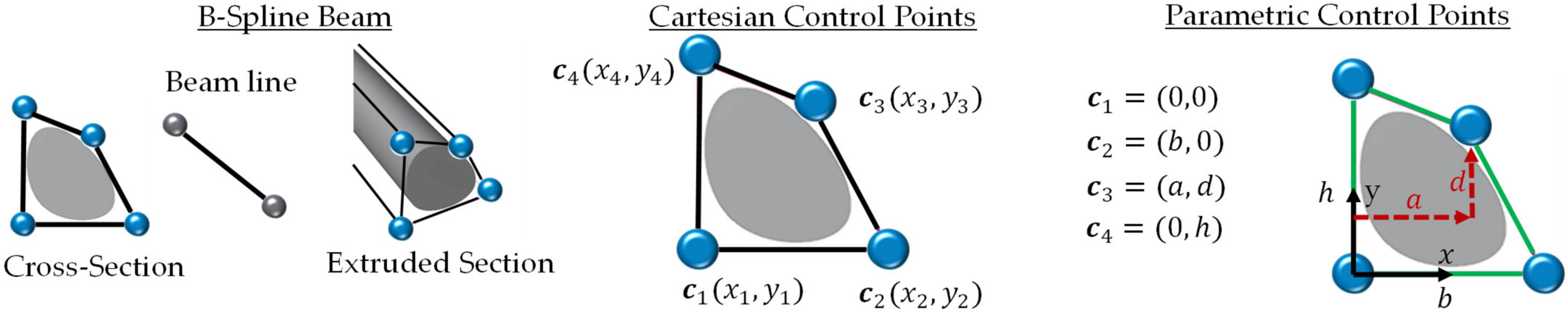
The advantage of constructive solid geometry (CSG) derived from circular and elliptical cross-sections includes the parametric representation of the curve and the moments of area, which are necessary for the evaluation of the bending stiffness as well as for FE simulations. For freeform cross-sections, the calculation of the moments is usually performed in a large number of numerically treated point coordinates, where they are determined via a boundary integral. In a recent publication [15], instead of a numerical calculation approach, a parametric formula was derived analytically, e.g., for the area of a triangle and rectangle control polygon. Figure 1 shows the example of a bar with Cartesian coordinates and with a parametric of the control polygon of a B-spline.

However, since, in [15], only a triangle and a rectangle are considered and a numerical estimation of the coefficients of the second moments of area is carried out, a parametric description of the moments of area is analyzed in the context of this work. On one hand, the zero- and second-order moments of area are determined analytically, and, on the other hand, in addition to the triangle and rectangle, various control polygons, such as the moments of area of a parallelogram, a trapeze, a symmetric pentagon, and a symmetric hexagon control polygon, are derived.

In addition to the determination of the equations for the moments, an extensive validation strategy is presented. First, the formulas are checked against correlations of valid cross-sections, so that, for example, the cross-sectional area must always be greater than 0. Then, the freeform curves are converted into polygons by an appropriate choice of control points and compared with results from the literature using a triangle and a rectangle as examples. Finally, a numerical comparison of the moments of area is performed with alternative calculation methods of the moments of polygons as well as of 2D binary images. This validation can be used to ensure the validity of the automatically calculated formulas.

In the following, the properties and the methods for the determination of the moments of area of periodic splines are described. Then, alternative methods for calculating moments of polygons and images are explained. Finally, the essential parameters of moments are described.

1.2. State of the Art

The parametric representation of various shapes and topologies has been discussed in various articles for simple polygons as common cross-section types [16,17] and also for more complex topologies consisting of multiple polygons such as hexagonal networks [18,19]. The knot positions of these for one or several polygons can be considered as control points for tensor product splines.

There are several different kinds of splines such as the Overhauser spline [20,21], the Catmull–Rom spline [22], B-splines [23], and Bezier splines [24]. These different spline types may differ in properties such as the convex hull criterion or the type of continuity [25]. The convex hull criterion describes the property in which, given a convex control polygon, the resulting spline lies within that control polygon. While B-splines provide $C^2$ continuity and the convex hull criterion, Bezier curves only guarantee $C^1$ continuity and the convex hull criterion [25]. Catmull–Rom splines are only $C^1$ continuous and violate the convex hull criterion [25]. The Catmull–Rom spline and the Bezier spline offer. in contrast to B-splines. the advantage that the control points are located on the curve. Due to the convex criterion and the $C^2$ continuity, this article focuses on B-splines. Such a cross-section can be used to describe 3D surfaces by using operations, such as skinning or sweeping, along a curve [26] to design, for example, a propeller blade [27]. Furthermore, B-splines can be used to model the mechanical behavior of a beam [15,28]. Additionally, they can be used in the structural optimization of lattices [15,29,30,31], so that the beam line or its cross-section changes due to some objective function.

The calculation of the moments of freeform curves has been performed in several publications [32,33,34]. The calculation is carried out via the boundary integral along the spline using Green’s Theorem in order to be able to calculate the moments of area directly [32,33]. This boundary integral can be traced back to a summation of the individual points, including weighting factors. The authors of [32] compared their equations using several B-splines to approximate the ellipse against the exact moments of area. While the authors of [32,33] considered the calculation on 2D shapes, the authors of [35] calculated the moment of inertia for the 3D shapes of freeform surfaces instead. Such moments of area, particularly for splines, are often used for shape matching [36,37] due to the invariant properties.

However, since this summation has a large number of coefficients, a more compact parametric description is often desirable. The authors of [15] were able to find an exact parametric description of triangles and rectangles for the value of the cross-sectional area, the formula of which was subsequently used for the truss optimization as well as the 3D reconstruction. In this work, analogous to [15], such a compact description shall be found for different control polygons and for different types of splines. In contrast to [15], a complete analytical description of the second order of the moments of area, as well as the transfer to control polygons consisting of a parallelogram, a trapeze, a symmetric pentagon, and a symmetric hexagon, is guaranteed.

In addition to the numerical calculation of spline cross-sections, alternative geometric representations such as a polygon or an image can also be used. The moments of binary images were investigated in several articles such as [16,38]. By summing up the single pixels to a rectangle, the area can be calculated by considering Steiner’s theorem and the center of area, and the second moments of area can be calculated with the following equations [16]:

$$A_{Img}={\displaystyle \sum }_{i\in B}1; S_{x_{Img}}={\displaystyle \sum }_{i\in B}{y}_i 1^2; S_{y_{Img}}={\displaystyle \sum }_{i\in B}{x}_i 1^2$$

(1)

$$I_{x_{Img}}={\displaystyle \sum }_{i\in B}\left(\frac{1}{12}+{\left(y_s-y_i\right)}^2\right); I_{y_{Img}}={\displaystyle \sum }_{i\in B}\frac{1}{12}+{\left(x_s-x_i\right)}^2; I_{x{y}_{Img}}=-{\displaystyle \sum }_{i\in B}\left(y_s-y_i\right)\left(x_s-x_i\right)$$

(2)

For polygonal cross-sections, the moments of area with respect to the center of area can be determined with the following equations [39,40]:

$$I_{x_{Poly}}=\frac{1}{12}{\displaystyle \sum }_i^n\left(y_i^2+y_i{y}_{i+1}+y_{i+1}^2\right) a_i$$

(3)

$$I_{y_{Poly}}=\frac{1}{12}{\displaystyle \sum }_i^n\left(x_i^2+x_i{x}_{i+1}+x_{i+1}^2\right)a_i$$

(4)

$$I_{x{y}_{Poly}}=-\frac{1}{24}{\displaystyle \sum }_i^n\left(x_i{y}_{i+1}+2x_i{y}_i+2x_{i+1}{y}_{i+1}+x_{i+1}{y}_i\right)a_i$$

(5)

$$a_i=x_i{y}_{i+1}-x_{i+1}{y}_i$$

(6)

Typically, cross-sections can be converted from algebraic curves to images or polygons directly. Therefore, it is reasonable to cross-validate the new equations to the alternative representations using Equations (1) and (2). While the equations of the polygon cross-section are determined by a boundary integration, the equations for the binary image were determined by an area integration. While these numerical approximations of the moments of area can be computed quite quickly, the main advantage of parametric cross-sections is their interpretability and direct use in algebraic equations. For example, the beam stiffness matrix can be constructed directly using the parametric spline description, which can be further optimized [15].

2. Materials and Methods

In order to determine the formulas for the moments, the description of a periodic B-spline is first explained in more detail. Then, based on the publication [32], the approach to derive the formulas for the analytical moments is presented. Finally, a suitable experimental setup is presented to automatically test the formulas numerically against alternative calculation methods as well as against general correlations of valid cross-sections. A tensor product spline describes a family of curves that can be represented [25,41] with

$$\mathit{P}\left(t\right)=\mathit{T}\mathit{M}\mathit{C}\mathbf{,}$$

(7)

where $\mathit{P}\left(t\right)$ describes the curve, $\mathit{T}$ describes the monomial basis, $\mathit{C}$ describes the control points of the spline, and $\mathit{M}$ describes the geometry matrix [25]. In the case of a cubic B-spline, the relationship for a segment can be described as follows:

$${\mathit{P}}_i\left(t\right)=\left(\begin{array}{c}x\left(t\right)\\ y\left(t\right)\end{array}\right)=\left[t^3 t^2 t 1\right]\frac{1}{6}\left[\begin{array}{cccc}-1& 3& -3& 1\\ 3& -6& 3& 0\\ -3& 0& 3& 0\\ 1& 4& 1& 0\end{array}\right]{\left[{\mathit{c}}_{i-1} {\mathit{c}}_i {\mathit{c}}_{i+1} {\mathit{c}}_{i+2}\right]}^T$$

(8)

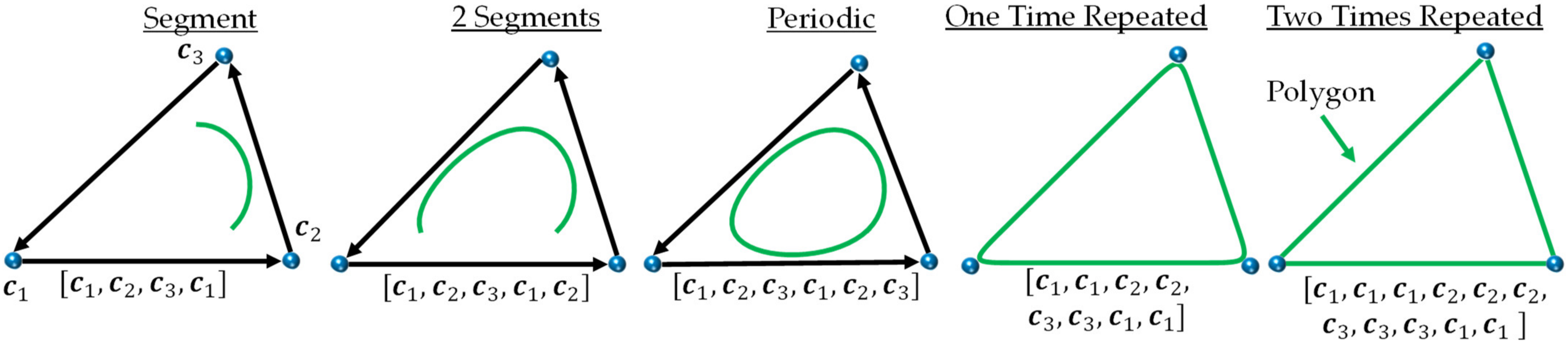
where ${\mathit{c}}_i$ is the individual control points and $t$ is the parametrization along the spline of the monomial basis. Figure 2 shows for a triangular control polygon the computation of the B-spline using different sequences of control points. A periodic B-spline can be obtained by repeating the first two control points. If the individual control points are repeated in the sequence itself, a sharper spline is obtained, and repeating twice gives the control polygon as a contour.

In this work, we restrict ourselves to periodic splines since they only lead to a closed cross-section. For the first validation, the moments of area of the control polygon calculated by repeating the control points must match with the moments of area of a directly computed polygon in Equation (2). Therefore, the moment formulas of a rectangle or triangle must match those from the approach with the B-spline.

2.1. Moments of Area of a Periodic B-Spline

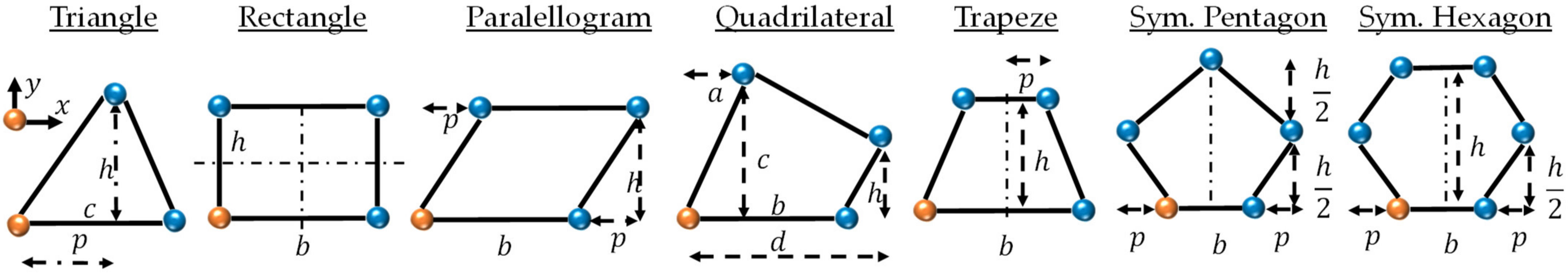
Different control polygons can be parametrized for the calculation of the moments of area. Figure 3 shows a variation of different control polygons with the parameters used in each case.

For the moments of splines, the authors of [32,33] used a boundary integral along the tensor product spline with $N$ control points and the coordinates $X_n, Y_n$ to calculate the area of such a spline with

$$A={\displaystyle \sum }_{i=0}^N{\displaystyle \sum }_l^4{\displaystyle \sum }_m^4{C}_{lm}{X}_{i+l-2}{Y}_{i+m-2}$$

(9)

where the coefficient $C_{lm}$ can be calculated by summing the geometry matrix [32] with:

$$C_{lm}={\displaystyle \sum }_{j=1}^4{\displaystyle \sum }_{k=1}^3\frac{M_{jl}{M}_{km}\left(4-k\right)}{8-j-k}.$$

(10)

Analogously, the first and second order moments were determined in [32] using the following equations:

$$S_x=\frac{-1}{2}{\displaystyle \sum }_{i=0}^N{\displaystyle \sum }_{l=1}^4{\displaystyle \sum }_{m=1}^4{\displaystyle \sum }_{n=1}^4{C}_{lmn}{Y}_{i+l-2}{Y}_{i+m-2}{X}_{i+o-2}$$

(11)

$$S_y=\frac{1}{2}{\displaystyle \sum }_{i=0}^N{\displaystyle \sum }_{l=1}^4{\displaystyle \sum }_{m=1}^4{\displaystyle \sum }_{n=1}^4{C}_{lmn} X_{i+l-2}{X}_{i+m-2}{X}_{i+n-2}{Y}_{i+o-2}$$

(12)

$$I_x=\frac{-1}{3}{\displaystyle \sum }_{i=0}^N{\displaystyle \sum }_{l=1}^4{\displaystyle \sum }_{m=1}^4{\displaystyle \sum }_{n=1}^4{\displaystyle \sum }_{o=1}^4{C}_{lmno}{Y}_{i+l-2}{Y}_{i+m-2}{Y}_{i+n-2}{X}_{i+o-2}$$

(13)

$$I_y=\frac{1}{3}{\displaystyle \sum }_{i=0}^N{\displaystyle \sum }_{l=1}^4{\displaystyle \sum }_{m=1}^4{\displaystyle \sum }_{n=1}^4{\displaystyle \sum }_{o=1}^4{C}_{lmno} X_{i+l-2}{X}_{i+m-2}{X}_{i+n-2}{Y}_{i+o-2}$$

(14)

$$I_{yz}=-\frac{1}{2}{\displaystyle \sum }_{i=0}^N{\displaystyle \sum }_{l=1}^4{\displaystyle \sum }_{m=1}^4{\displaystyle \sum }_{n=1}^4{\displaystyle \sum }_{o=1}^4{C}_{lmno} X_{i+l-2}{X}_{i+m-2}{Y}_{i+n-2}{Y}_{i+o-2}$$

(15)

The coefficients $C_{lmn}$ and $C_{lmno}$ can be calculated as follows [32]:

$$C_{lmn}={\displaystyle \sum }_{j=1}^4{\displaystyle \sum }_{k=1}^4{\displaystyle \sum }_{r=1}^3\frac{M_{jl}{M}_{km}{M}_{rn}\left(4-r\right)}{12-j-k-r}$$

(16)

$$C_{lmno}={\displaystyle \sum }_{j=1}^4{\displaystyle \sum }_{k=1}^4{\displaystyle \sum }_{r=1}^4{\displaystyle \sum }_{s=1}^3\frac{M_{jl}{M}_{km}{M}_{rn}{M}_{so}\left(4-s\right)}{16-j-k-r-s}$$

(17)

With the help of these equations, the parametric descriptions of the control polygons can be generated. In the following, the parametrization is determined schematically for a triangular control polygon.

2.2. Parametric Representation of the B-Spline of a Triangle

Based on the parametric in Figure 3, the area can now be determined. For a B-spline, the area can be calculated as follows:

$$A=\frac{1}{36}\left[-\frac{9}{20} ch-\frac{15}{2}hp-\frac{9}{10}ch-\frac{1}{2}hp+\frac{1}{20}hp-\frac{19}{10}ch+\frac{71}{20}ch-\frac{1}{20}hp+\frac{1}{2}hp+\frac{183}{20}ch+\frac{15}{2}hp\right]$$

(18)

This results in an expression similar to that found in [15]:

$$A=21 c\frac{h}{80}.$$

(19)

Analogously, the first and second order moments of area with respect to the coordinate origin can be calculated with

$$S_x^{\left(0,0\right)}=7 c\frac{h^2}{80}$$

$$S_y^{\left(0,0\right)}=7\frac{c^{2}h}{80}+7 c h\frac{p}{80}$$

$$I_{xx}^{\left(0,0\right)}=15769 c\frac{h^3}{443520}$$

$$I_{yy}^{\left(0,0\right)}=15769\frac{c^{3}h}{443520}+23039 c^{2}h\frac{p}{443520}+15769 c h\frac{p^2}{443520}$$

$$I_{xy}^{\left(0,0\right)}=-23039\frac{c^2{h}^2}{887040}-15769 c\frac{h^{2}p}{443520}.$$

From the first moments of area, the center of area of the spline cross-section can now be calculated with

$$x_s=\frac{S_y}{A}=\frac{c}{3}+\frac{p}{3}$$

(20)

$$y_s=\frac{S_x}{A}=h/3.$$

(21)

Using the center of area, the second order moments can now be referenced to the center of area with

$$I_{xx}=I_{xx}^{\left(0,0\right)}-y_s^{2}A=\frac{2833}{443520}c{h}^3$$

(22)

$$I_{yy}=I_{yy}^{\left(0,0\right)}-x_s^{2}A=\frac{2833}{443520}c h\left(c^2-c p+p^2\right)$$

(23)

$$I_{xy}=I_{xy}^{\left(0,0\right)}+x_s{y}_{s}A=2833 c\frac{h^2\left(c-2 p\right)}{887040}.$$

(24)

It is noticeable that the structure of the moments of the B-spline differs from that of a triangle only in the coefficients (see also

Table 1. List of symbols and abbreviations.

TSP	Tensor Product Spline	CSG	Constructive Solid Geometry
$C^1$	Tangential Continuity	$A$	Zeroth Moment of Area (Cross-Sectional Area)
$C^2$	Curvature Continuity	$S_x, S_y$	First Moment of Area
$\mathit{T}$	Monomial Basis	$I_x, I_y,I_{xy}$	Second Moment of Area
$\mathit{M}$	Geometry Matrix	$A_{Img}, I_{x_{Img}}$  $I_{y_{Img}},I_{x{y}_{Img}}$	Moments of Area of the Binary Image
${\mathit{C}}_i$	Control Point of the Tensor Product Spline	$A_{Poly}, I_{x_{Poly}}$  $I_{y_{Poly}},I_{x{y}_{Poly}}$	Moments of Area of the Polygon
$\mathit{P}\left(t\right)$	Tensor Product Spline	$A_{yy}^{\left(0,0\right)}, I_{yy}^{\left(0,0\right)}$  $I_{xy}^{\left(0,0\right)},I_{xx}^{\left(0,0\right)}$	Moments of Area referred to the Origin of the Coordinate System
$x_s,y_s$	Center Points of the Cross-Section	$A_{TPS}, I_{x_{TPS}}$  $I_{y_{TPS}},I_{x{y}_{TPS}}$	Moments of Area of the Tensor Product Spline
$c,b,h,p,a,d$	Geometric Sizes	$I_1,I_2$	Principal Moments of Area
$B$	Binary Image	${ϵ}_A,{ϵ}_{I_{xy}},{ϵ}_{I_x},{ϵ}_{I_y}$	Relative Errors
$\sigma ²$	Variance	$\overline{{ϵ}_{[\dots ]}}$	Mean Value of $[\dots ]$

). To check the validity of the formulas found for the moments, it is necessary to compare them with alternative calculation methods and to check valid cross-section properties.

2.3. Comparison to Polygon Cross-Sections

By repeating the control points, the B-spline formula can be used to accurately reproduce the shape of a polygon and, therefore, its moments of area. If the parametric formula is derived from this, the moment of area formula of, for example, a rectangle or a triangle is obtained in

Table 2. Derivation of the moments of area using the equations for the B-spline.

	Triangle	Rectangle
$A$	$c\frac{h}{2}$	$bh$
$I_x$	$c\frac{h^3}{36}$	$b\frac{h^3}{12}$
$I_y$	$c h\frac{c^2-c p+p^2}{36}$	$\frac{b^{3}h}{12}$
$I_{xy}$	$c\frac{h^2\left(c-2 p\right)}{72}$	$0$
$x_s,y_s$	$\left(\frac{c}{3}+\frac{p}{3},\frac{h}{3}\right)$	$\left(\frac{b}{2},\frac{h}{2}\right)$

. The following table shows the determination of the moments via the B-spline formula, which can also be derived from Equation (2) or found in the literature [1].

The comparison with the table shows an agreement of the calculation methods with the literature. Thus, it can be seen that if the control points (polygon) are repeated twice, the results from the literature can be determined directly.

2.4. Numerical Comparison Framework

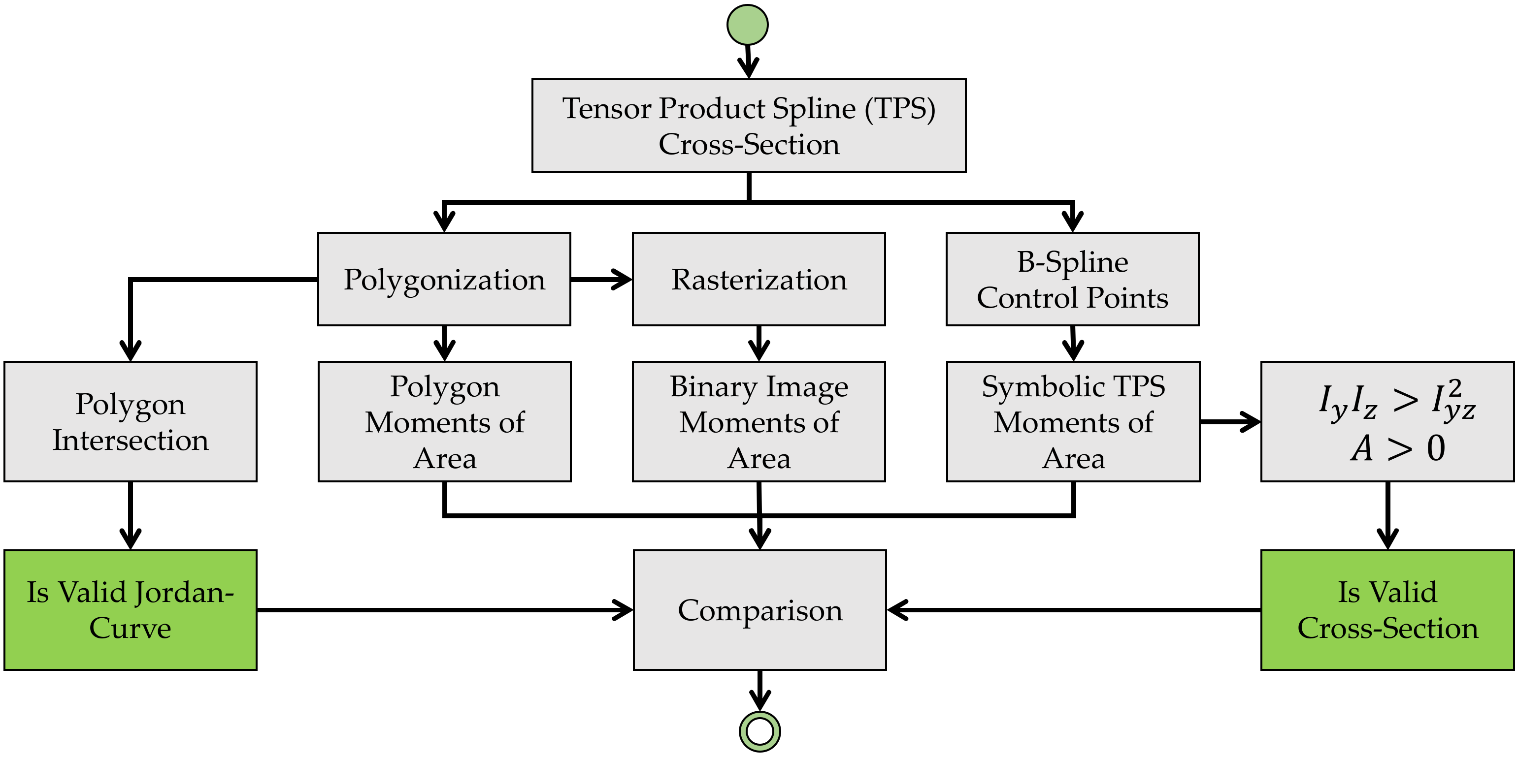
To ensure the validity of the formulas with a high degree of accuracy, they must be validated with alternative calculation methods and by checking the Jordan curve theorem and valid cross-section properties. Figure 4 shows the steps involved in the automatic validation of the equations for the cross-sections. First, a tensor product spline is defined. This curve is then converted into a discrete polygon and the control polygon points. From the control polygon points, the parametric equation is derived and the numerical results of the moments are then compared to the moments of the polygon as well as the moments from a binary image.

In addition, for each formula it is checked whether it is a valid cross-section or a curve, as determined by the Jordan curve theorem.

2.4.1. Spline Cross-Section with Valid Cross-Section Property

A valid cross-section has a positive cross-sectional area and positive principal axis moments (eigenvalues), so that all combinations of parameters must fulfill

$$A>0 \wedge I_1>0 \wedge I_2>0$$

(25)

Principal moments can be computed with

$$I_{1,2}=\frac{I_y+I_z}{2}\pm \sqrt{{\left(\frac{I_y-I_z}{2}\right)}^2+I_{yz}^2}>0.$$

However, since this expression can be very complex, it is first necessary to find a simplified criterion for valid cross-sections. It is sufficient to state that the smaller principal moment of area given by

$$I_2=\frac{I_y+I_z}{2}-\sqrt{{\left(\frac{I_y-I_z}{2}\right)}^2+I_{yz}^2}>0$$

must be greater than zero. This leads to

$$\frac{I_y+I_z}{2}>\sqrt{{\left(\frac{I_y-I_z}{2}\right)}^2+I_{yz}^2}$$

$$I_y^2+2I_y{I}_z+I_z^2>I_y^2-2I_y{I}_z+I_z²+4I_{yz}^2$$

$$I_y{I}_z>I_{yz}^2.$$

Therefore, for all parameter combinations, a valid cross-section has to fulfill

$$A>0 \wedge I_y{I}_z-I_{yz}^2>0$$

(26)

In addition to the relationship between the moments of area for valid cross-sections, it is also necessary to compare the formula found with various alternative calculation methods.

2.4.2. Spline Cross-Section as Valid Jordan Curve

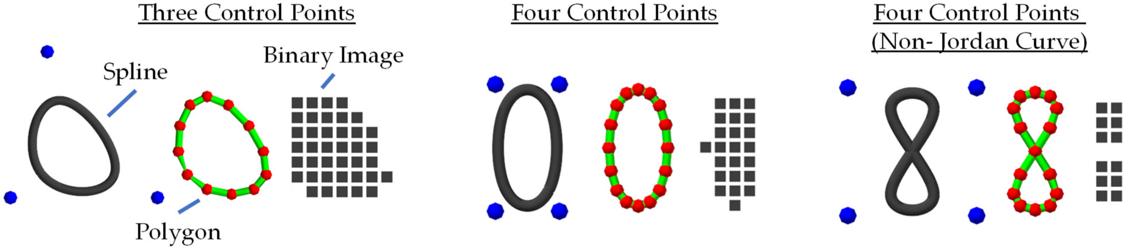
For validation, the spline is converted into a polygon and into a 2D binary image. Then, the moments can be calculated in different ways for the particular spline. Figure 4 shows three different B-splines, their polygons (red and green), and a binary image of their cross-sections.

A comparison of Equations (1) and (2) is used to check the accuracy and validity. As the number of segments along the polygon line is increased, the accuracy of the moments of area estimate also increases. The comparison with the formula of the binary image serves to ensure the validity of the calculated curve, so that no Jordan curves are detected. Figure 5 shows a non-Jordan curve by swapping the order of the nodes. While such a cross-section can be estimated with some accuracy using the binary image, the boundary integration approach using the polygon approach, as well as the chosen formula derived for the B-spline, leads to incorrect results (e.g., area = 0, in this case).

To achieve a high degree of coverage, it is necessary to compare the approach with a large number of possible polygon and binary image cross-sections. For each parametrization, a Latin hypercube sampling is chosen by generating a large number of cross-sections. Then, the mean error and the variance of the error are chosen as evaluation criteria in comparison to the alternative computational methods. For this purpose, the relative errors are determined as follows.

2.4.3. Spline Cross-Section Numerically Compared to Polygon and Image Cross-Section

To validate each formula, the moments from the derived polygon cross-section and the image $A_{Img, Poly}$, $I_x{}_{Img, Poly}$, $I_y{}_{Img, Poly}$, $I_{xy}{}_{Img, Poly}$ are compared with the moments of the B-spline formula $A_{TPS},$ $I_x{}_{TPS},$ $I_y{}_{TPS}$, $I_{xy}{}_{TPS}$. Thereby, the relative errors of a large number of combinations of the control polygons, including

$${ϵ}_A=\left|\frac{A_{Img, Poly}-A_{TPS}}{A_{TPS}}\right|$$

(27)

$${ϵ}_{I_x}=\left|\frac{I_x{}_{Img, Poly}-I_x{}_{TPS}}{A_{TPS}}\right|$$

(28)

$${ϵ}_{I_y}=\left|\frac{I_y{}_{Img, Poly}-I_y{}_{TPS}}{I_y{}_{TPS}}\right|$$

(29)

$${ϵ}_{I_{xy}}=\left|\frac{I_{xy}{}_{Img, Poly}-I_{xy}{}_{TPS}}{I_{xy}{}_{TPS}}\right|$$

(30)

can be compared. Possible geometric values can be selected in the range of the geometric space, such as, for example, for a triangle between

$$c\in \left[0,\infty \left[, h\in \right[0,\infty \left[, p\in \right[0,\infty \right[.$$

Thus, each individual geometric variable and its influence can be checked directly. However, since an evaluation up to ∞ is not possible, a limiting parameter of the geometric variable of 100.0 is chosen. For each case, 100 samples are generated using Latin Hypercube Sampling.

3. Results

Based on the described strategy for the parametrization as well as for the evaluation of the found formulas, it is necessary in the following to design different parametric control points for the tensor product splines. From these parametric control point coordinates, the respective moments are then calculated automatically and analytically. In this work, the moments of a general triangle, a rectangle, a trapeze, a parallelogram, an isosceles pentagon, and an isosceles hexagonal honeycomb are considered, since, for these parametric quantities, there is a suitable simple expression, which can still be presented on a few lines.

For the evaluation of these moments of area, the approach from Section 2.4 is chosen. By using the Jordan curve theorem, the parametric is restricted so that only valid Jordan curves are used as cross-section results.

Table 3. Example of three cases of different control polygons as B-splines and alternative representations as six-line segment polygons along the curve and as 8 × 8 binary images.

Control Polygon	Case 1 $\mathbf{b}=1, \mathbf{p}=0.75, \mathbf{h}=1.5$	Case 2 $\mathbf{b}=1, \mathbf{p}=2.0, \mathbf{h}=2.5$	Case 3 $\mathbf{b}=1, \mathbf{p}=0.1, \mathbf{h}=0.5$
Triangle
Rectangle
Parallelogram
Trapeze
Pentagon
Hexagon

shows for different control polygon types several cases with different parameters (see also Figure 3). For comparison, the resulting curve was rasterized into an 8 × 8 pixel image and segmented into a polygon consisting of six segments.

3.1. Moments of Area Parametrization of a Triangle Control Polygon

Since the triangle itself is always a convex polygon, the curve also lies within the selected polygon. The value of the area must, therefore, be smaller than that of the triangle itself.

Table 4. Equations for the parametric control polygon for the triangle and its numerical error.

	Equation	Error [%]	${\mathit{P}}_{100}$	${\mathit{P}}_{10}$	${\mathit{I}}_{128}$	${\mathit{I}}_{16}$
$A$	$21 c\frac{h}{80}$	$\overline{{ϵ}_A}$	0.007	0.879	1.922	11.951
$I_x$	$2833 c\frac{h^3}{443520}$	$\sigma ²\left({ϵ}_A\right)$	0.000	0.000	0.168	4.990
$I_y$	$2833 c h\frac{c^2-c p+p^2}{443520}$	$\overline{{ϵ}_{I_x}}$	0.015	1.776	4.299	19.075
$I_{xy}$	$2833 c\frac{h^2\left(c-2 p\right)}{887040}$	$\sigma ²\left({ϵ}_{I_x}\right)$	0.000	0.000	0.810	5.377
$x_s,y_s$	$\left(\frac{c}{3}+\frac{p}{3},\frac{h}{3}\right)$	$\overline{{ϵ}_{I_y}}$	0.015	1.776	3.247	18.471
$I_x{I}_y-I_{xy}^2$	$8025889\frac{c^4{h}^4}{262279987200}$	$\sigma ²\left({ϵ}_{I_y}\right)$	0.000	0.000	0.291	5.914
		$\overline{{ϵ}_{I_{xy}}}$	0.015	1.776	5.046	25.759
		$\sigma ²\left({ϵ}_{I_{xy}}\right)$	0.000	0.000	1.575	6.264

shows the formulas for calculating the moments of area and the relative errors compared to a polygon with 100 segments, a polygon with 10 segments per spline segment, an image $I_{128}$ with a grid size of 128 × 128 pixels, and an image $I_{16}$ with a grid size of 16 × 16 pixels.

Equation (26) always shows values greater than zero for the geometric parameters of $c, h$; thus, the essential properties for a valid cross-section are guaranteed for positive geometric parameters. The relative error from the calculation shows an average relative error of 0.015% for $P_{100}$. This error increases when fewer segments per spline $P_{10}$ are used. The errors for binary images are significantly higher compared to the polygon approach. Furthermore, if a 16 × 16 pixel grid is chosen, an error of 25.7% can occur for the second order moment of area.

The relative errors show good agreement between the different calculation methods, so that the formulas from Table 1 can be assumed to be correct. In particular, the small error for a high resolution of the spline as polygon $P_{100}$ shows good agreement.

3.2. Moments of Area Parametrization of a Quadrilateral Control polygon Area

For a quadrangular control polygon, the cross-sectional area of the B-spline can be generally expressed as

$$A=-61 a\frac{h}{180}+61 b\frac{h}{180}+61 c\frac{d}{180}$$

(31)

according to the parametrization covered in Figure 3. However, the parametrization of the general quadrilateral can lead to the violation of the Jordan curve theorem, so that the curve can intersect itself. This can lead to a negative cross-sectional area, so that more appropriate boundary conditions for the dependencies of the parameters of the control polygon have to be considered for a robust application. In the following, the quadrilateral is constructed as a rectangle, a trapeze, and a parallelogram.

3.2.1. Moments of Area Parametrization of a Rectangle Control Polygon

Due to the chosen parametrization of a rectangle, only positive and valid cross-sections can be realized compared to the general quadrilateral.

Table 5. Equations for the parametric control polygon for the rectangle and its relative error.

	Equation	Error [%]	${\mathit{P}}_{100}$	${\mathit{P}}_{10}$	${\mathit{I}}_{128}$	${\mathit{I}}_{16}$
$A$	$61 b\frac{h}{90}$	$\overline{{ϵ}_A}$	0.004	0.505	2.674	13.488
$I_x$	$27371 b\frac{h^3}{748440}$	$\sigma ²\left({ϵ}_A\right)$	0.000	0.000	1.110	5.877
$I_y$	$27371\frac{b^{3}h}{748440}$	$\overline{{ϵ}_{I_x}}$	0.008	1.009	3.858	16.736
$I_{xy}$	$0$	$\sigma ²\left({ϵ}_{I_x}\right)$	0.000	0.000	1.473	6.440
$x_s,y_s$	$\left(\frac{b}{2},\frac{h}{2}\right)$	$\overline{{ϵ}_{I_y}}$	0.008	1.009	3.687	17.262
$I_x{I}_y-I_{xy}^2$	$749171641\frac{b^4{h}^4}{560162433600}$	$\sigma ²\left({ϵ}_{I_y}\right)$	0.000	0.000	1.248	5.963

shows the equations for the moments of area of the rectangular control polygon as well as the numerical errors. Analogous to the triangle, a high accuracy of the relative errors is again shown in comparison to the polygonal approach. Similarly, it can be seen that Equation (26) leads exclusively to positive values. The moment of area of $I_{xy}$ leads to a value of 0 due to the symmetric shape of the control polygon.

3.2.2. Moments of Area Parametrization of a Parallelogram Control Polygon

Table 6. Equations for the parametric control polygon for the triangle and its numerical error.

	Equation				Error [%]	${\mathit{P}}_{100}$	${\mathit{P}}_{10}$	${\mathit{I}}_{128}$	${\mathit{I}}_{16}$
$A$	$61 a\frac{h}{90}$				$\overline{{ϵ}_A}$	0.004	0.505	2.218	12.118
$I_x$	$27371 b\frac{h^3}{748440}$				$\sigma ²\left({ϵ}_A\right)$	0.000	0.000	1.075	4.609
$I_y$	$27371 b h\frac{b^2+p^2}{748440}$				$\overline{{ϵ}_{I_x}}$	0.008	1.009	3.831	19.453
$I_{xy}$	$-27371 b\frac{h^{2}p}{748440}$				$\sigma ²\left({ϵ}_{I_x}\right)$	0.000	0.000	1.489	5.294
$x_s,y_s$	$\left(\frac{b}{2}+\frac{p}{2},\frac{h}{2}\right)$				$\overline{{ϵ}_{I_y}}$	0.008	1.009	3.463	20.586
$I_x{I}_y-I_{xy}^2$	$749171641\frac{b^4{h}^4}{560162433600}$				$\sigma ²\left({ϵ}_{I_y}\right)$	0.000	0.000	1.298	5.750
					$\overline{{ϵ}_{I_{xy}}}$	0.008	1.009	4.474	30.458
					$\sigma ²\left({ϵ}_{I_{xy}}\right)$	0.000	0.000	1.920	9.431

shows the results for the moments of area of the control polygon as a parallelogram as well as the numerical errors. Analogous to the triangle, a high accuracy of the relative errors is also shown here in comparison to the polygonal approach. Similarly, it can be seen that Equation (26) leads exclusively to positive values. The moment of area $I_{xy}$ is 0 for the parallelogram with $p=0,$ which represents a rectangle. Otherwise, this leads to values unequal to 0 due to the asymmetry of the cross-section.

3.2.3. Moments of Area Parametrization of a Trapeze Control Polygon

For the validity of the trapezoids, according to Equation (26), the following relation is positive and, therefore, valid for each possible parameter combination:

$$\begin{gathered} I_x{I}_y-I_{xy}^2=\frac{{\mathrm{h}}^4\left(75371706005{ \mathrm{b}}^4+564591208444{ \mathrm{b}}^3\mathrm{p} \right)}{820077802790400}+ \\ \frac{{\mathrm{h}}^4\left(1525810647880{ \mathrm{b}}^2{\mathrm{p}}^2+2258364833776{ \mathrm{b} \mathrm{p}}^3+1205947296080{ \mathrm{p}}^4\right)}{820077802790400} \end{gathered}$$

(32)

Table 7. Equations for the parametric control polygon for the rectangle and its relative error.

	Equation	Error [%]	${\mathit{P}}_{100}$	${\mathit{P}}_{10}$	${\mathit{I}}_{128}$	${\mathit{I}}_{16}$
$A$	$61 h\frac{b+2 p}{180}$	$\overline{{ϵ}_A}$	0.004	0.505	0.915	9.991
$I_x$	$\frac{h^3\left(4412605 b^2+22420724 b p+17650420 p^2\right)}{273929040 \left(b+2 p\right)}$	$\sigma ²\left({ϵ}_A\right)$	0.000	0.000	0.013	3.937
$I_y$	$h\frac{17081 b^3+75322 b^{2}p+150644 b p^2+136648 p^3}{2993760}$	$\overline{{ϵ}_{I_x}}$	0.008	0.961	2.180	15.232
$I_{xy}$	$0$	$\sigma ²\left({ϵ}_{I_x}\right)$	0.000	0.000	0.132	4.967
$x_s,y_s$	$\left(\frac{b}{2}; h\frac{461 b+1274 p}{1098 \left(b+2 p\right)}\right)$	$\overline{{ϵ}_{I_y}}$	0.009	1.097	1.385	13.110
$I_x{I}_y-I_{xy}^2$	$\left(32\right)$	$\sigma ²\left({ϵ}_{I_y}\right)$	0.000	0.000	0.002	4.336

shows the results for the moments of area of the control polygon as a trapeze as well as the numerical errors. Analogous to the triangle, a high accuracy of the relative errors is also shown in comparison to the polygonal approach. The moment $I_{xy}$ is consistently zero due to the symmetry. For the parameter $p=\frac{b}{2}$, the relation of the rectangle is obtained.

In an analogous way, further quadrilaterals can now be parametrized and their formulas for the moments of area can be derived. In the following, the calculation of the moments of area of a parametric pentagon, as well as of a hexagon, is performed.

3.3. Moments of Area Parametrization of a Symmetric Pentagon Control Polygon

For the validity of the pentagon, according to Equation (19), the following relation leads to only positive values:

$$\begin{gathered} I_x{I}_y-I_{xy}^2=\frac{{\mathrm{h}}^4\left(82305438169{ \mathrm{b}}^2+212310520756 \mathrm{b} \mathrm{p} +120438027736{ \mathrm{p}}^2\right)}{ \left(169 \mathrm{b} +218 \mathrm{p}\right)}· \\ \frac{\left(1527254{ \mathrm{b}}^3+5667223{ \mathrm{b}}^2\mathrm{p} +7684452{ \mathrm{b} \mathrm{p}}^2+3712596{ \mathrm{p}}^3\right)}{963658637770752000} \end{gathered}$$

(33)

Table 8. Equations for the parametric control polygon for the rectangle and its relative error.

	Equation	Error [%]	${\mathit{P}}_{100}$	${\mathit{P}}_{10}$	${\mathit{I}}_{128}$	${\mathit{I}}_{16}$
$A$	$h\frac{169 b+218 p}{288}$	$\overline{{ϵ}_A}$	0.003	0.332	2.438	14.852
$I_x$	$\frac{h^3\left(82305438169 b^2+212310520756 b p+120438027736 p^2\right)}{20118067200 \left(169 b+218 p\right)}$	$\sigma ²\left({ϵ}_A\right)$	0.000	0.000	1.298	6.766
$I_y$	$h\frac{1527254 b^3+5667223 b^{2}p+7684452 b p^2+3712596 p^3}{47900160}$	$\overline{{ϵ}_{I_x}}$	0.005	0.643	4.220	19.337
$I_{xy}$	$0$	$\sigma ²\left({ϵ}_{I_x}\right)$	0.000	0.000	1.454	7.039
$x_s,y_s$	$\left(\frac{b}{2}; h\frac{167189 b+254368 p}{2520 \left(169 b+218 p\right)}\right)$	$\overline{{ϵ}_{I_y}}$	0.006	0.690	2.291	17.653
$I_x{I}_y-I_{xy}^2$	$\left(33\right)$	$\sigma ²\left({ϵ}_{I_y}\right)$	0.000	0.000	1.276	7.541

shows the results for the moments of area of the control polygon as a symmetric pentagon as well as the numerical errors. Analogous to the triangle, the relative errors also show a high accuracy compared to the polygonal approach. The moment $I_{xy}$ is consistently zero due to the symmetry.

Finally, the parametrization for a hexagon can now be specified analogously.

3.4. Moments of Area Parametrization of a Symmetric Hexagonal Control Polygon

A valid hexagonal has to fulfill the following equation:

$$\begin{gathered} I_x{I}_y-I_{xy}^2=\frac{{\mathrm{h}}^4\left(1267299 \mathrm{b} +927031 \mathrm{p}\right)}{143401583001600}· \\ \left(354311{ \mathrm{b}}^3+1131397{ \mathrm{b}}^2\mathrm{p} +1267299{ \mathrm{b} \mathrm{p}}^2+490213{ \mathrm{p}}^3\right) \end{gathered}$$

(34)

Table 9. Equations for the parametric control polygon for the rectangle and its relative error.

	Equation	Error [%]	${\mathit{P}}_{100}$	${\mathit{P}}_{10}$	${\mathit{I}}_{128}$	${\mathit{I}}_{16}$
$A$	$301 h\frac{b+p}{360}$	$\overline{{ϵ}_A}$	0.002	0.225	1.128	15.193
$I_x$	$\frac{h^3\left(1267299 b+927031 p\right)}{23950080}$	$\sigma ²\left({ϵ}_A\right)$	0.000	0.000	0.081	7.610
$I_y$	$h\frac{354311 b^3+1131397 b^{2}p+1267299 b p^2+490213 p^3}{5987520}$	$\overline{{ϵ}_{I_x}}$	0.003	0.398	2.405	20.943
$I_{xy}$	$0$	$\sigma ²\left({ϵ}_{I_x}\right)$	0.000	0.000	0.419	8.302
$x_s,y_s$	$\left(\frac{b}{2},\frac{h}{2}\right)$	$\overline{{ϵ}_{I_y}}$	0.004	0.511	1.037	15.814
$I_x{I}_y-I_{xy}^2$	$\left(34\right)$	$\sigma ²\left({ϵ}_{I_y}\right)$	0.000	0.000	0.037	7.627

shows the results for the moments of area of the control polygon as a symmetric hexagon as well as the numerical errors. Analogous to the triangle, the relative errors also show a high accuracy compared to the polygonal approach. The moment $I_{xy}$ is consistently zero due to the symmetry.

4. Discussion

The final formulas show a very good suitability for the design and determination of beams with freeform cross-sections. In particular, the comparison of the formulas with alternative calculation methods suggests a high validity.

One point of criticism could be the chosen parametrization of the control polygons. While the triangle was still covered for arbitrary shapes, there are already restrictions for the moment of area for a quadrilateral due to the complexity of the perpetual expressions. The same is true for pentagons and hexagons. Only a restriction of the parametric allows simpler expressions, e.g., for a parallelogram as well as a trapeze. However, this simplification can be improved to achieve high shape coverage with a suitable set of variables. For example, the parametric of the positive lengths of the symmetric hexagon yields exclusively convex polygons, so this unfavorable choice implicitly excludes many alternative symmetric hexagons.

While the numerical formula for determining the moments of area is easy to implement and universally applicable, the symbolic expressions lead to the restriction of the cross-sectional geometry. However, due to the numerical accuracy of such formulas, erroneous moments of area cannot be absolutely guaranteed, unlike in the analytical formula. The symbolic expressions can be used completely up to the limit ranges, so that a consideration of the convergence behavior towards infinity is also possible. Especially in the case of optimization, cross-section values close to zero can occur, at which point a numerical approximation can lead do misleading results.

The validation framework exhibits high robustness and reliability, so that symbolic formulas can be tested directly. However, for future work, the estimation of a polygon consisting of many segments is usually sufficient. Unlike the polygon and the B-spline, the binary image and the evaluation step is based on an area integral rather than a boundary integral and is, therefore, not directly comparable.

In summary, however, a large number of expressions are shown, which can be used to determine moments of area of such freeform curves in the simplest way. These can now not only be used for aspects of structural optimization, but also for reconstructions analogous to [15]. In contrast to [15], however, a fully analytical function of the beam stiffness matrix can be realized, so that geometric values close to zero can be accurately captured.

5. Conclusions

This work has dealt with the derivation of analytical formulas for the moments of area of periodic B-splines. The position of the control points was mapped parametrically and then embedded in the boundary integral for the calculation of the moments of area of splines. In contrast to common methods for the numerical determination of moments of area, a symbolic calculation with an integer numerator and denominator was considered. This integer calculation leads to an exact determination of the cross-sectional area and the second moments of area of such periodic B-spline cross-sections.

While, in [15], only the cross-sectional area was determined analytically, in this work, a symbolic description for the second moments of area could be obtained. Especially in structural optimization, cross-section parameters close to zero can be determined, for which an exact calculation of the moments is necessary.

The obtained expressions can now be used for various applications in the field of reconstruction design, as well as in verification calculations. Similarly, further control polygons can be parametrized using the approach described above.

References

- Gross, D.; Hauger, W.; Schröder, J.; Wall, W.A. (Eds.) Balkenbiegung. In Technische Mechanik 2: Elastostatik; Springer: Berlin/Heidelberg, Germany, 2017; pp. 81–165. [Google Scholar] [CrossRef]
- Bendsoe, M.P.; Sigmund, O. Topology Optimization: Theory, Methods, and Applications, 2nd ed.; Springer: Berlin/Heidelberg, Germany, 2004. [Google Scholar] [CrossRef]
- Changizi, N.; Warn, G.P. Topology optimization of structural systems based on a nonlinear beam finite element model. Struct. Multidiscip. Optim. 2020, 62, 2669–2689. [Google Scholar] [CrossRef]
- Denk, M.; Rother, K.; Gadzo, E.; Paetzold, K. Multi-Objective Topology Optimization of Frame Structures Using the Weighted Sum Method. In Proceedings of the Munich Symposium on Lightweight Design 2021; Springer: Berlin/Heidelberg, Germany, 2022; pp. 83–92. [Google Scholar] [CrossRef]
- Fredricson, H.; Johansen, T.; Klarbring, A.; Petersson, J. Topology optimization of frame structures with flexible joints. Struct. Multidiscip. Optim. 2003, 25, 199–214. [Google Scholar] [CrossRef]
- Lim, J.; You, C.; Dayyani, I. Multi-objective topology optimization and structural analysis of periodic spaceframe structures. Mater. Des. 2020, 190, 108552. [Google Scholar] [CrossRef]
- Denk, M.; Rother, K.; Paetzold, K. Multi-Objective Topology Optimization of Heat Conduction and Linear Elastostatic using Weighted Global Criteria Method. In DS 106: Proceedings of the 31st Symposium Design for X (DFX2020); The Design Society: Bamberg, Germany, 2020; pp. 91–100. [Google Scholar] [CrossRef]
- Stangl, T.; Wartzack, S. Feature based interpretation and reconstruction of structural topology optimization results. In DS 80-6 Proceedings of the 20th International Conference on Engineering Design (ICED 15) Vol 6: Design Methods and Tools—Part 2 Milan, Italy, 27–30.07.15; Weber, C., Husung, S., CantaMESsa, M., Cascini, G., Marjanovic, D., Graziosi, S., Eds.; Design Society: Glasgow, UK, 2015; Volume 6, pp. 235–245. [Google Scholar]
- Nana, A.; Cuillière, J.-C.; Francois, V. Automatic reconstruction of beam structures from 3D topology optimization results. Comput. Struct. 2017, 189, 62–82. [Google Scholar] [CrossRef]
- Tang, P.-S.; Chang, K.-H. Integration of topology and shape optimization for design of structural components. Struct. Multidiscip. Optim. 2001, 22, 65–82. [Google Scholar] [CrossRef]
- Denk, M.; Klemens, R.; Paetzold, K. Beam-colored Sketch and Image-based 3D Continuous Wireframe Reconstruction with different Materials and Cross-Sections. In Entwerfen Entwickeln Erleben in Produktentwicklung und Design 2021; Stelzer, R., Krzywinski, J., Eds.; TUDpress: Dresden, Germany, 2021; pp. 345–354. [Google Scholar] [CrossRef]
- Denk, M.; Rother, K.; Paetzold, K. Fully Automated Subdivision Surface Parametrization for Topology Optimized Structures and Frame Structures Using Euclidean Distance Transformation and Homotopic Thinning. In Proceedings of the Munich Symposium on Lightweight Design 2020; Pfingstl, S., Horoschenkoff, A., Höfer, P., Zimmermann, M., Eds.; Springer: Berlin/Heidelberg, Germany, 2021; pp. 18–27. [Google Scholar] [CrossRef]
- Amroune, A.; Cuillière, J.-C.; François, V. Automated Lofting-Based Reconstruction of CAD Models from 3D Topology Optimization Results. Comput. Aided Des. 2022, 145, 103183. [Google Scholar] [CrossRef]
- Piegl, L.; Tiller, W. The NURBS Book. In Monographs in Visual Communications; Springer: Berlin/Heidelberg, Germany, 1995. [Google Scholar] [CrossRef]
- Denk, M. Curve Skeleton and Moments of Area Supported Beam Parametrization in Multi-Objective Compliance Structural Optimization. Ph.D. Dissertation, Technische Universität Dresden, Saxony, Germany, 2022. Available online: https://nbn-resolving.org/urn:nbn:de:bsz:14-qucosa2-822020 (accessed on 12 February 2023).
- Denk, M.; Rother, K.; Höfer, T.; Mehlstäubl, J.; Paetzold, K. Euclidian Distance Transformation, Main Axis Rotation and Noisy Dilitation Supported Cross-Section Classification with Convolutional Neural Networks. In Proceedings of the Design Society; Cambridge University Press: Cambridge, UK, 2021; Volume 1, pp. 1401–1410. [Google Scholar] [CrossRef]
- Denk, M.; Rother, K.; Neuhäusler, J.; Petroll, C.; Paetzold, K. Parametrization of Cross-Sections by CNN Classification and Moments of Area Regression for Frame Structures. In Proceedings of the Munich Symposium on Lightweight Design 2021, Online, 6 August 2022; Springer: Berlin/Heidelberg, Germany, 2022; pp. 93–103. [Google Scholar] [CrossRef]
- Azeem, M.; Jamil, M.K.; Shang, Y. Notes on the Localization of Generalized Hexagonal Cellular Networks. Mathematics 2023, 11, 844. [Google Scholar] [CrossRef]
- Nadeem, M.F.; Azeem, M. The fault-tolerant beacon set of hexagonal Möbius ladder network. Math. Methods Appl. Sci. 2023. [Google Scholar] [CrossRef]
- Overhauser, A.W. Analytic Definition of Curves and Surfaces by Parabolic Blending. arXiv 2005, arXiv:cs/0503054. [Google Scholar]
- El-Abbasi, N.; Meguid, S.A.; Czekanski, A. On the modelling of smooth contact surfaces using cubic splines. Int. J. Numer. Methods Eng. 2001, 50, 953–967. [Google Scholar] [CrossRef]
- Catmull, E.; Rom, R. A CLASS OF LOCAL INTERPOLATING SPLINES. In Computer Aided Geometric Design; Barnhill, R.E., Riesenfeld, R.F., Eds.; Academic Press: Cambridge, MA, USA, 1974; pp. 317–326. [Google Scholar] [CrossRef]
- Curry, H.B.; Schoenberg, I.J. On Pólya frequency functions IV: The fundamental spline functions and their limits. J. Anal. Math. 1966, 17, 71–107. [Google Scholar] [CrossRef]
- Borisenko, V.V. Construction of Optimal Bézier Splines. J. Math. Sci. 2019, 237, 375–386. [Google Scholar] [CrossRef]
- Clark, J.H. Parametric Curves, Surfaces and Volumes in Computer Graphics and Computer-Aided Geometric Design; Technical Report; Stanford University: Stanford, CA, USA, 1981. [Google Scholar] [CrossRef]
- Woodward, C.D. Cross-sectional design of B-spline surfaces. Comput. Graph. 1987, 11, 193–201. [Google Scholar] [CrossRef]
- Pérez-Arribas, F.; Pérez-Fernández, R. A B-spline design model for propeller blades. Adv. Eng. Softw. 2018, 118, 35–44. [Google Scholar] [CrossRef]
- Capobianco, G.; Eugster, S.R.; Winandy, T. Modeling planar pantographic sheets using a nonlinear Euler–Bernoulli beam element based on B-spline functions. PAMM 2018, 18, e201800220. [Google Scholar] [CrossRef]
- Goel, A.; Anand, S. Design of Functionally Graded Lattice Structures using B-splines for Additive Manufacturing. Procedia Manuf. 2019, 34, 655–665. [Google Scholar] [CrossRef]
- Weeger, O. Isogeometric sizing and shape optimization of 3D beams and lattice structures at large deformations. Struct. Multidiscip. Optim. 2022, 65, 43. [Google Scholar] [CrossRef]
- Zhang, L.; Feih, S.; Daynes, S.; Wang, Y.; Wang, M.Y.; Wei, J.; Lu, W.F. Buckling optimization of Kagome lattice cores with free-form trusses. Mater. Des. 2018, 145, 144–155. [Google Scholar] [CrossRef]
- Rozenthal, P.; Gattass, M. Geometrical properties in the B-spline representation of arbitrary domains. Commun. Appl. Numer. Methods 1987, 3, 345–349. [Google Scholar] [CrossRef]
- Sheynin, S.; Tuzikov, A. Moment computation for objects with spline curve boundary. IEEE Trans. Pattern Anal. Mach. Intell. 2003, 25, 1317–1322. [Google Scholar] [CrossRef]
- Sheynin, S.; Tuzikov, A. Area and Moment Computation for Objects with a Closed Spline Boundary. In Computer Analysis of Images and Patterns; Petkov, N., Westenberg, M.A., Eds.; Springer: Berlin/Heidelberg, Germany, 2003; pp. 33–40. [Google Scholar] [CrossRef]
- Soldea, O.; Elber, G.; Rivlin, E. Exact and efficient computation of moments of free-form surface and trivariate based geometry. Comput. Des. 2002, 34, 529–539. [Google Scholar] [CrossRef]
- Huang, Z.; Cohen, F. Affine-invariant B-spline moments for curve matching. IEEE Trans. Image Process. 1996, 5, 1473–1480. [Google Scholar] [CrossRef] [PubMed]
- Jacob, M.; Blu, T.; Unser, M. An exact method for computing the area moments of wavelet and spline curves. IEEE Trans. Pattern Anal. Mach. Intell. 2001, 23, 633–642. [Google Scholar] [CrossRef]
- Flusser, J.; Suk, T. On the Calculation of Image Moments; Institute of Information Theory and Automation, Academy of Sciences of the Czech Republic: Prague, Czechia, 1999. [Google Scholar]
- Soerjadi, R. On the Computation of the Moments of a Polygon, with Some Applications; Delft University of Technology: Delft, The Netherlands, 1968. [Google Scholar]
- Hally, D. Calculation of the Moments of Polygons; Technical Report ADA183444; Defense Technical Information Center: Fort Belvoir, VA, USA, 1987. [Google Scholar]
- Botsch, M.; Kobbelt, L.; Pauly, M.; Alliez, P.; Lévy, B. Polygon Mesh Processing; CRC Press: Boca Raton, FL, USA, 2010. [Google Scholar]
Figure 1.
B-spline beam: Cross-section and centerline beam; Cartesian coordinates of control points; parametric coordinates of contour points.
Figure 2.
Variation of the number of control points: B-spline segment; two segments; periodic B-spline; sharped one time repeated B-spline; polygon.
Figure 3.
Parametrization of the control polygon: triangle; rectangle; parallelogram; quadrilateral; trapeze; symmetric pentagon; symmetric hexagon.
Figure 4.
Framework for the validation of the symbolic equations of the moments of area.
Figure 5.
Tensor product spline cross-sections (B-splines) and their polygons and binary images.