Variation of Elastic Stiffness Parameters of Granitic Rock during Loading in Uniaxial Compressive Test


1
Dept. Engng, Geol. & Geotechn., Faculty of Civil Engng, Budapest University of Technology and Economics, 1111 Budapest, Hungary
2
RockStudy Ltd., 7633 Pécs, Hungary
*
Author to whom correspondence should be addressed.
Appl. Mech. 2023, 4(2), 445-459; https://doi.org/10.3390/applmech4020025
Submission received: 7 March 2023
/
Revised: 7 April 2023
/
Accepted: 12 April 2023
/
Published: 13 April 2023
Abstract
:Any rock mechanics’ design inherently involves determining the deformation characteristics of the rock material. The purpose of this study is to offer equations for calculating the values of bulk modulus (K), elasticity modulus (E), and rigidity modulus (G) throughout the loading of the sample until failure. Also, the Poisson’s ratio, which is characterized from the stress–strain curve, has a significant effect on the rigidity and bulk moduli. The results of a uniaxial compressive (UCS) test on granitic rocks from the Morágy (Hungary) radioactive waste reservoir site were gathered and examined for this purpose. The fluctuation of E, G, and K has been the subject of new linear and nonlinear connections. The proposed equations are parabolic in all of the scenarios for the Young’s modulus and shear modulus, the study indicates. Furthermore, the suggested equations for the bulk modulus in the secant, average, and tangent instances are also nonlinear. Moreover, we achieved correlations with a high determination factor for E, G, and K in three different scenarios: secant, tangent, and average. It is particularly intriguing to observe that the elastic stiffness parameters exhibit strong correlation in the results.
1. Introduction
For virtually any type of design and analysis in geomechanical projects, a precise assessment of the geomechanical properties of rocks is essential. [1,2,3,4,5,6,7] are only a few of the researchers who have researched the strength and deformation behavior of rocks. Among these characteristics, the bulk modulus (K), modulus of rigidity (G), and modulus of elasticity (E) are the fundamental variables employed in rock engineering. The moduli can be calculated using either destructive or nondestructive techniques. In the destructive one, the moduli are derived from the rock material’s stress–strain curves. This is a feature of the elasticity modulus.
In general, it is possible to determine the parameters of rock mass deformability, including the Young’s modulus, through field tests essentially as in situ moduli (signified by Erm) directly and through research lab tests as intact modulus (signified by E) indirectly. It is important to evaluate the characteristics of rock deformation using both field and lab conditions because accurate deformation analysis of rock must be undertaken due to location-specific factors. [8].
The Poisson’s ratio (ν) is an elastic constant with a largely underappreciated significance in comparison to the other fundamental mechanical characteristics of rocks. There are many different areas in rock mechanics that need prior information or an estimate of the Poisson’s ratio (ν); these areas are spread out and are quite numerous. Rock engineering can benefit from the knowledge of various Poisson’s ratio features. In accordance with [9], the Poisson’s ratio of rocks remains constant during linear elastic deformation but starts to rise as a result of the emergence of new microcracks or the growth of pre-existing ones.
In rock mechanics and rock engineering, the bulk modulus (K) of a rock is an important physical property that can provide insights into the rock’s behavior under different conditions. For example, it can be used to predict how much a rock will compress under the weight of overlying rock layers or to calculate the density of the Earth’s crust. It is also used in the design of structures that are built into or on top of rocks, such as dams or tunnels, to ensure that they are resistant to compression and other forms of stress.
The shear modulus (G), also known as the modulus of rigidity, is a measure of a material’s resistance to deformation under shear stress. In the case of rocks, the shear modulus is a measure of how much the rock will deform when subjected to a certain amount of shear stress. Rocks with higher shear moduli are generally more resistant to deformation and less likely to undergo significant shear strain.
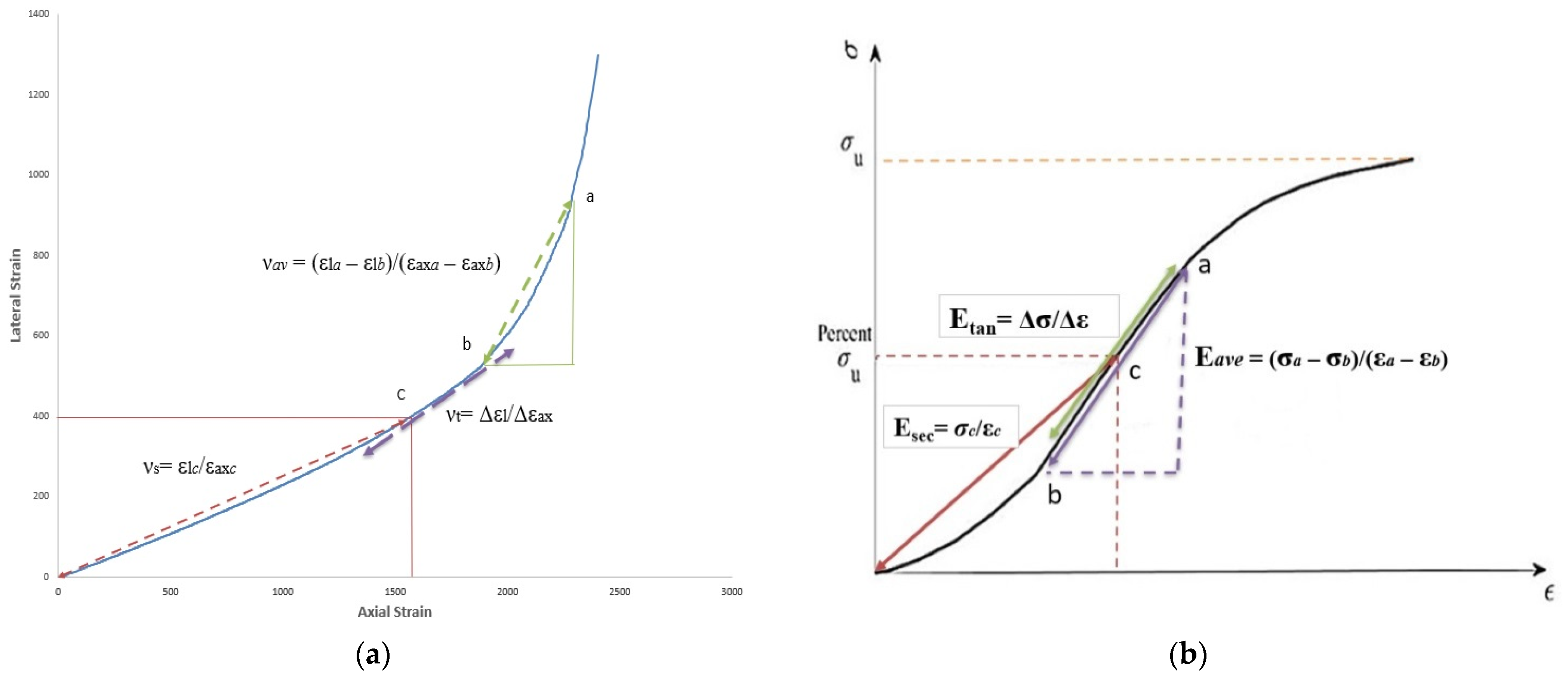
The most effective method for evaluating rock elasticity is calculating the Poisson’s ratio and the elastic modulus from the stress–strain curve. The stress–strain curve depicts the breakdown of a rock sample. By analyzing the shape of the curve, we may calculate the values of both mechanical and energy characteristics. It describes uniaxial testing carried out in various load systems and tests carried out in a complicated stress state. The International Society for Rock Mechanics suggested the following techniques to determine the Young’s modulus (E) and Poisson’s ratio (ν) of intact rock (see Figure 1) [10,11]:
The origin of the secant Poisson’s ratio was maintained at the zero-stress position, but the reference point was considered a moving point that changes with stress in order to analyze the behavior of the secant Poisson’s ratio. The secant Young’s modulus (Es) is defined as the slope of the line from the origin to some fixed percentage of ultimate strength. The average Poisson’s ratio reflects the relative change in axial and radial strain at the upper and lower limits of some stress interval. The average Young’s modulus (Eav) of the straight-line part of a curve is defined as the slope of the straight-line part of the stress–strain curve for the given test. The axial strain-lateral strain curve’s tangential slope is represented by the tangent Poisson’s ratio. The tangent Poisson’s ratio calculation is more susceptible to changes in the testing procedure and sample frequency than the secant Poisson’s ratio calculation. The tangent Young’s modulus (Et) is defined as the slope of a line tangent to the stress–strain curve at a fixed percentage of ultimate strength.
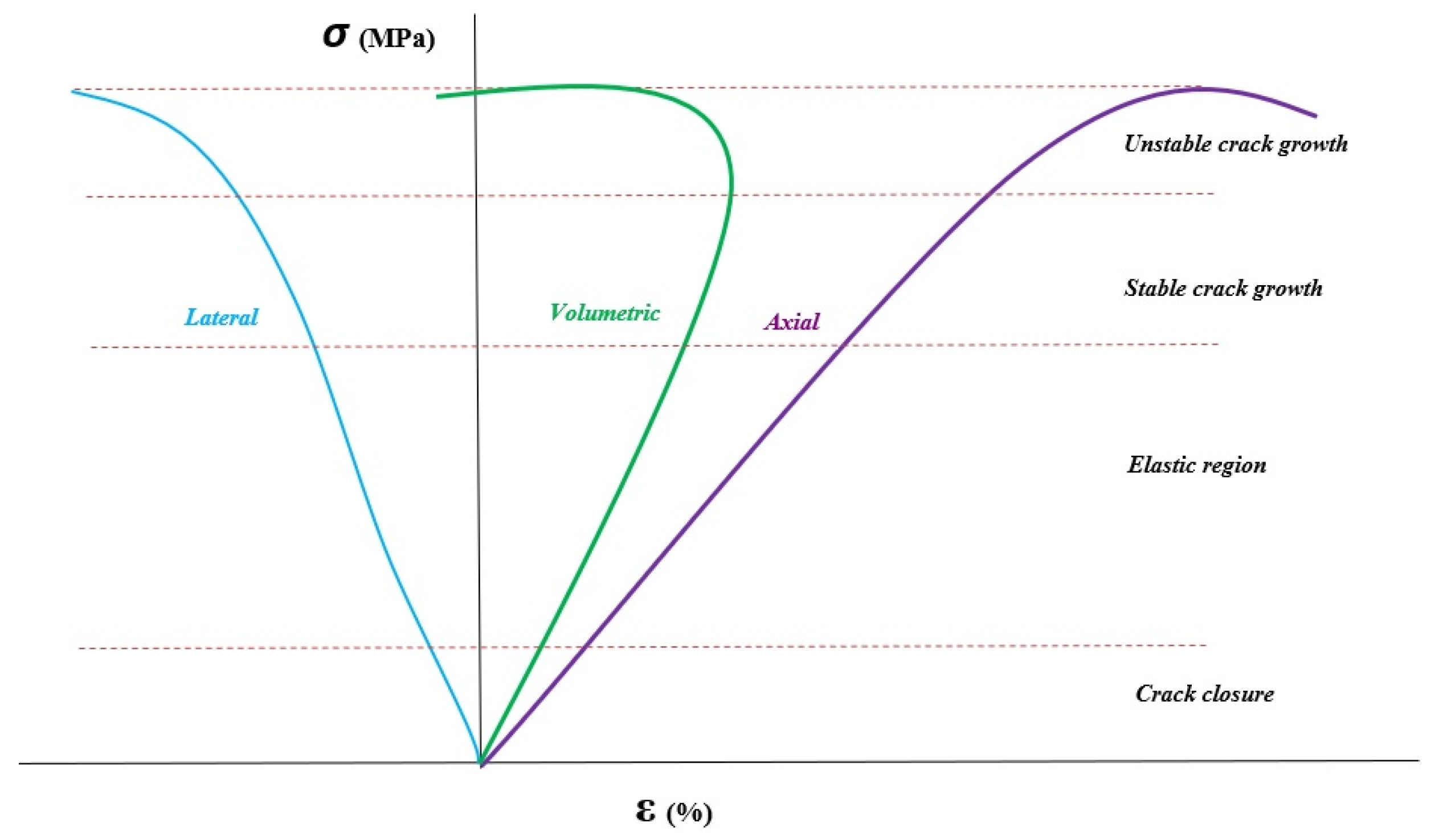
The assumption that applies to solids when discussing their mechanical behavior is that they are homogenous, continuous, and isotropic [12,13]. Nevertheless, rocks are significantly more complex, and their mechanical properties vary depending on scale, mineral composition, or matrix type. Engineers, however, typically need certain values of rock characteristics for different rock types. These can only be obtained by intensive laboratory and field research. Uniaxial compressive strength (UCS) is a geomechanical rock parameter that describes the maximum axial load that the sample can withstand without lateral loading. This is why it is also called uniaxial compressive strength. With regard to the uniaxial compressive strength, the rock can be classified as very weak to strong. Every rock exhibits elastic behavior up until a point where propagating cracks cause the deformation to become quasi-plastic. At this point, a rock has reached its peak strength and begins to degrade, changing the qualities of its strength. Pre-failure rock deformation typically goes through four stages [14] (see Figure 2).
- Crack closure phase: At increasing strain, the main joints and cracks as well as the inter-grain pores close. Because of the density and form of the main micro fractures, the stress–strain curve might be either linear or non-linear.
- Elastic region: Although non-linear behavior is possible, elastic deformations predominate in this phase. Linearity exists in the stress–strain curve.
- Stable crack growth: The micro-dilation limit, where the separation of cracks and their propagation in directions perpendicular to the main compressive stress direction marks the beginning of this phase, is when the cracks first start to spread. Transversal and volumetric deformations result in nonlinear stress–strain curves.
- Unstable crack growth: Surpassing the macro dilatancy limit causes the crack opening mode to start followed by the starting of the crack sliding mode and the spread of its unstable state. The shear surface is formed as a result of the cracks growing and connecting, which is observed in the quick increase in rock volume. There is a nonlinearity in all of the stress–strain curves. After the stress reaches its maximum intensity, the phase is finished.
Nearly all commercial numerical modeling systems for stress and deformation assessments now employ the Young’s modulus of intact rock, which has been used for the last decade. As an illustration, knowledge of stress concentrations and deformation is essential for the design of underground nuclear waste repositories in the granitic rocks of Mórágy (Hungary) [15]. The deformation behavior and its link to various stress levels, such as crack initiation stress, crack damage stress, and failure stress, are the main topics of their research. Unexpectedly, fresh, helpful correlations were found. Another influencing factor that can affect the elastic characteristics of the rock for trustworthy design is rock fracture [16]. When a specimen is slowly loaded, elastic characteristics can be assessed statically or dynamically, where the elasticity can be computed using the elastic-wave velocity [17].
There is no generally accepted theoretical equations or approaches to estimate the E, G, and K of intact rock during loading. The goal of this study is to ascertain how the elastic stiffness parameters, such as the Young’s modulus, shear modulus, and bulk modulus, change for intact granitic rocks as they progress through the UCS test from crack closure to failure stage. In the UCS test, we examine the values and fluctuations of the E, G, and K under three different conditions: secant, average, and tangent.
2. Methods and Results
One of the most crucial mechanical characteristics of rocks is their uniaxial compressive strength (UCS), which is frequently utilized in engineering-related projects to assess the stability of structures under loads. Due to the occurrence of weak, fractured, and foliated rocks, good quality core samples are required for the determination of the UCS but are not always available. The UCS tests were carried out according to the suggestion of the International Society for Rock Mechanics (ISRMRE) [11].
The tests were conducted using a computer-controlled, servo-hydraulic machine that was set to operate in continuous load control mode. During the tests, the samples were loaded with a high level of precision with an accuracy of 0.01 kN and at a constant rate of 0.6 kN/s. To measure the deformations experienced by the samples, both axial and lateral strain gauges were utilized. It is worth noting that the cylindrical rock samples adhered to the L/D ratio of 2/1, where L represented the length and D represented the diameter of each sample. In total, seventeen uniaxial compressive tests were performed in the rock mechanics laboratory.
The Poisson’s ratio is defined as the ratio of the radial strain and the corresponding axial strain caused by uniformly distributed axial stress [18]:
where ν is the Poisson’s ratio, εtrans is the transverse strain, and εaxial is the axial strain (positive strain indicates contraction, and negative strain indicates extension). The Poisson’s ratio is affected by a rock’s mineralogy and texture and can provide insights into a rock’s compressibility and deformation behavior. Theoretically, the Poisson’s ratio of isotropic and linear elastic material is a constant between −1 and +0.5. For rock materials, it is always positive and between 0.05 and 0.40.
The mechanical characteristic that gauges a material’s stiffness is known by several names, including the Young’s modulus, rigidity modulus, and bulk modulus. The Young’s modulus is the ratio of the material’s applied stress to the strain that results from that stress. According to [19], the Young’s modulus can be determined using Hook’s Law as follows:
For each type of rock, the Young’s modulus varies; its value is influenced by factors, such as the rock’s porosity, lithology, temperature, pore pressure, fluid saturation, and rock consolidation [20]. Furthermore, Davarpanah et al. [21] reviewed in great detail the impact of freezing on fundamental mechanical properties, such as the Young’s modulus, by determining density, ultrasound speed propagation, and strength parameters, and they discovered that the Young’s modulus rises as temperature falls.
A material’s resistance to hydrostatic compression is indicated by its bulk modulus (K). Its formula states that it is the ratio of a rise in pressure that is infinitesimally small to the volume that results from that pressure decrease. The bulk modulus K < 0 is officially defined in Equation (3) as follows:
P is for pressure, and V stands for volume, while dP/dV represents the pressure change in relation to volume. The formula below can be used to get the bulk modulus (K) with knowledge of the Young’s modulus (E) and Poisson’s ratio (ν):
The response of the material to shear stress is described by the shear modulus (G) or modulus of rigidity. It can be calculated using the formula below:
Several methods can be used to determine the elastic moduli of engineering materials. The initial tangent modulus, the tangent modulus of the straight-line portion of the stress–strain curve, the tangent modulus at a fixed percentage of maximum strength, the initial secant modulus (to maximum strength), the secant modulus at a fixed percentage of maximum strength, the average modulus, the loading modulus, and the unloading modulus are some of the techniques. There is a significant amount of research on the use of the Young’s modulus in rock, but none of it examines how the Young’s modulus changes when stress increases to the point of failure [22]. So, the other aim of this work is to find the best equations for each method of measuring elastic, shear, and bulk moduli in granitic rocks to compute changes in the elastic stiffness parameters. The tangent, secant, and average Young’s moduli were contrasted in a recent work by Malkowski et al. [23]. According to their research, the tangent Young’s modulus should be used as the guiding parameter at a fixed range of 30–70% of the ultimate load. It is appropriate to refer to the secant Young’s modulus—which ranges from 0 to 50% of the ultimate stress—as the modulus of deformability because it accounts for both elastic strain and pore compaction. In order to provide a reasonable estimate of the Young’s modulus of grain-supported carbonate rocks, Brievac et al. [24] used machine learning technology and took into account petrographic characteristics; however, they did not look into the variation of E. In addition, Davarpanah et al. [16] examined the linear correlations between several elastic parameters and the strength of the intact rock, including the Young’s modulus, shear modulus, and bulk modulus, for intact stratified rocks.
Many instances demonstrate how arbitrary the method used to calculate the Young’s modulus is. The research focuses on the effects of fissures or voids [17], porosity, mineral assemblage, water content, and permeability [10,25,26,27,28], as well as the correlations between the Young’s modulus and other physical parameters [25,26,27,28,29]. However, they pay little attention to determining the Young’s modulus or any other stiffness characteristics throughout the loading process from the beginning to the failure phase.
We conducted uniaxial compression tests on the Morágy granitic rock formation in Hungary in order to investigate the variation of the E, G, and K with a new method and formulation from the crack closure stage through failure stage.
2.1. Young’s Modulus and Shear Modulus
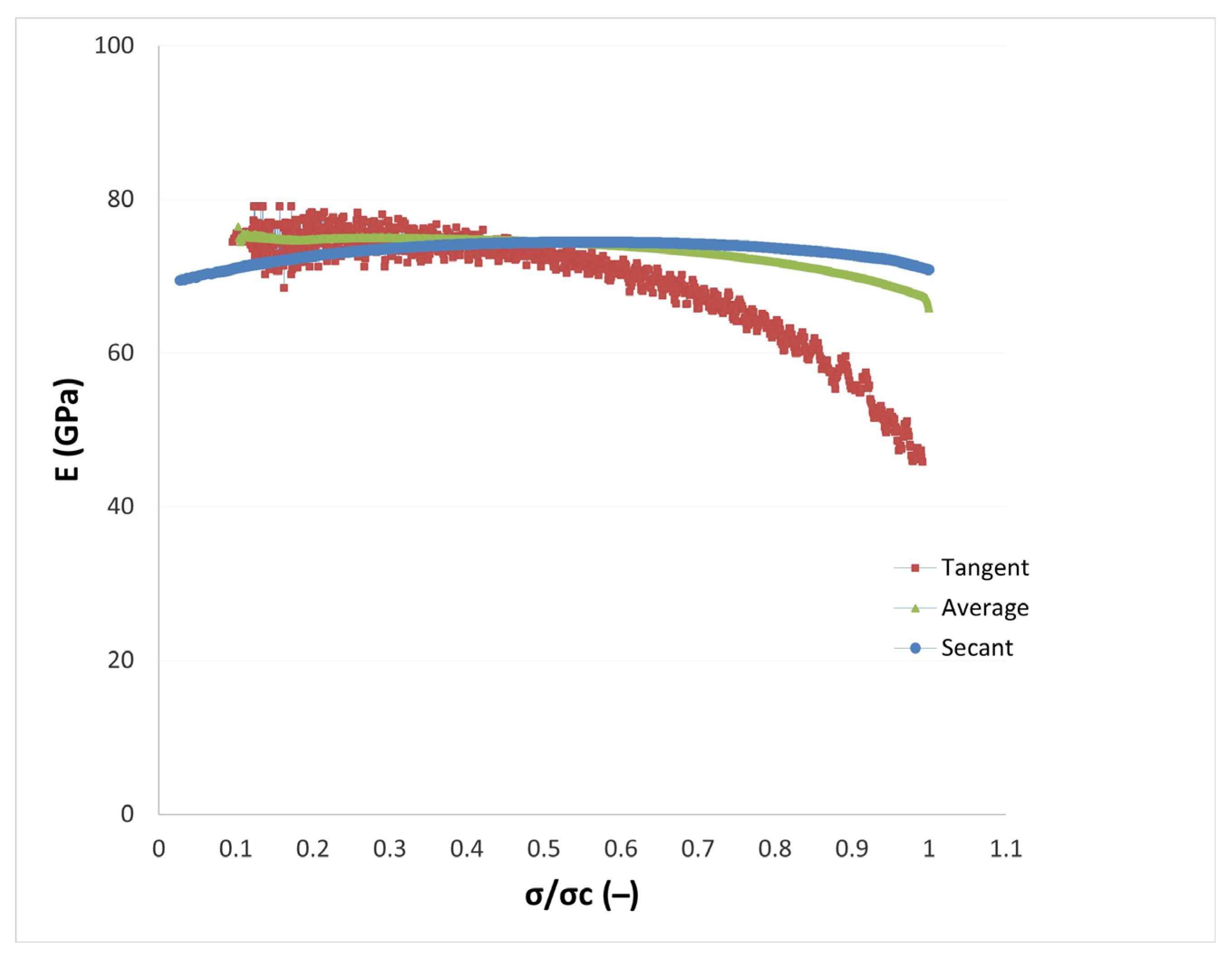
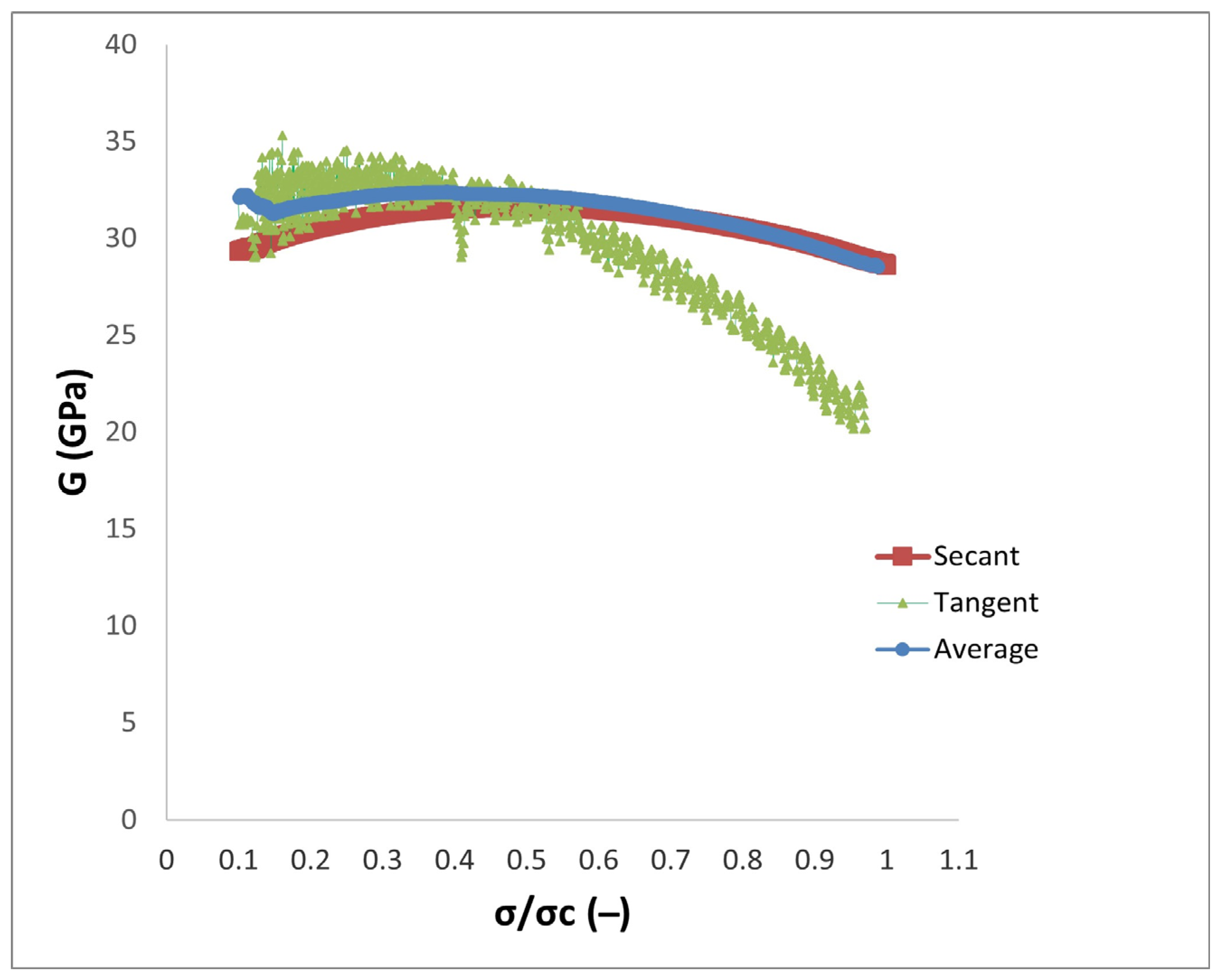
The analysis of the rock’s progressive deformation process is invariably negatively impacted by the method’s uncertainty and the resultant calculation uncertainty. After analyzing seventeen granitic specimens, the typical elastic modulus-σ/σc and shear modulus-σ/σc curves for granitic specimens in the uniaxial compressive strength test are shown in Figure 3 and Figure 4.
After our investigation, new quadratic equations were given to illustrate the link between σ/σc and the Young’s modulus and between σ/σc and the shear modulus in various scenarios since all of the generated curves adhere to the parabolic form. In each of these equations, there are three independent constants: a, b, and c. Table 1 and Table 2 report the obtained range for these constants for the Young’s modulus and shear modulus, respectively.
To be more specific, based on Figure 3, the behavior of the secant and average Young’s modulus from crack closure to the failure phase is approximately similar to each other. However, the tangent Young’s modulus shows different behavior. In other words, starting from crack closure through 60% of σ/σc, it demonstrates a similar trend to the secant and average Young’s modulus; after that and until the failure stage, it shows a significant divergence and decreases as the σ/σc increases.
In terms of the rigidity modulus of intact rock, the role of the Poisson’s ratio can be more significant. As indicated in Figure 4, the data is more widely scattering from crack closure through 50% of σ/σc. Similar to the Young’s modulus curves, the behavior of the secant and average shear modulus follow the same trend. Nevertheless, in the case of the tangent shear modulus, a big difference can be observed, and a substantial decrease of the tangent shear modulus occurs from 50% of σ/σc until the failure stage. This phenomenon is more probably associated with the variation of the tangent Poisson’s ratio.
2.2. Bulk Modulus
A new technique is presented to show how the bulk modulus values vary from crack closure to failure stage in the uniaxial compressive test. This approach results in a scale of stress over peak stress (σ/σc) that ranges between −80 and +80, where σ/σc = 0 and 1 accordingly. To do this, a new proposed model was fitted to the experimental graph based on Equation (6) with the origin of the coordinate system for all seventeen granitic specimens changed to σ/σc = 0.5 to provide a symmetrical condition.
K = K0.5 + (3K0.5) tan(degree)/B
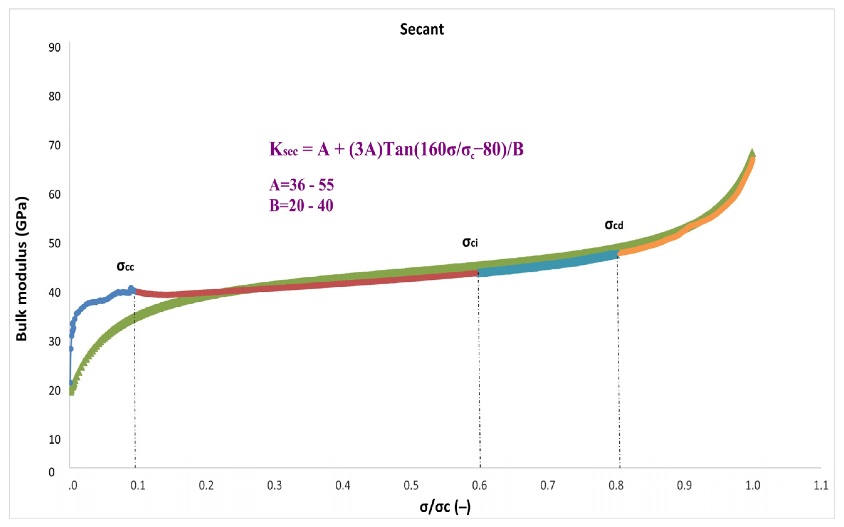
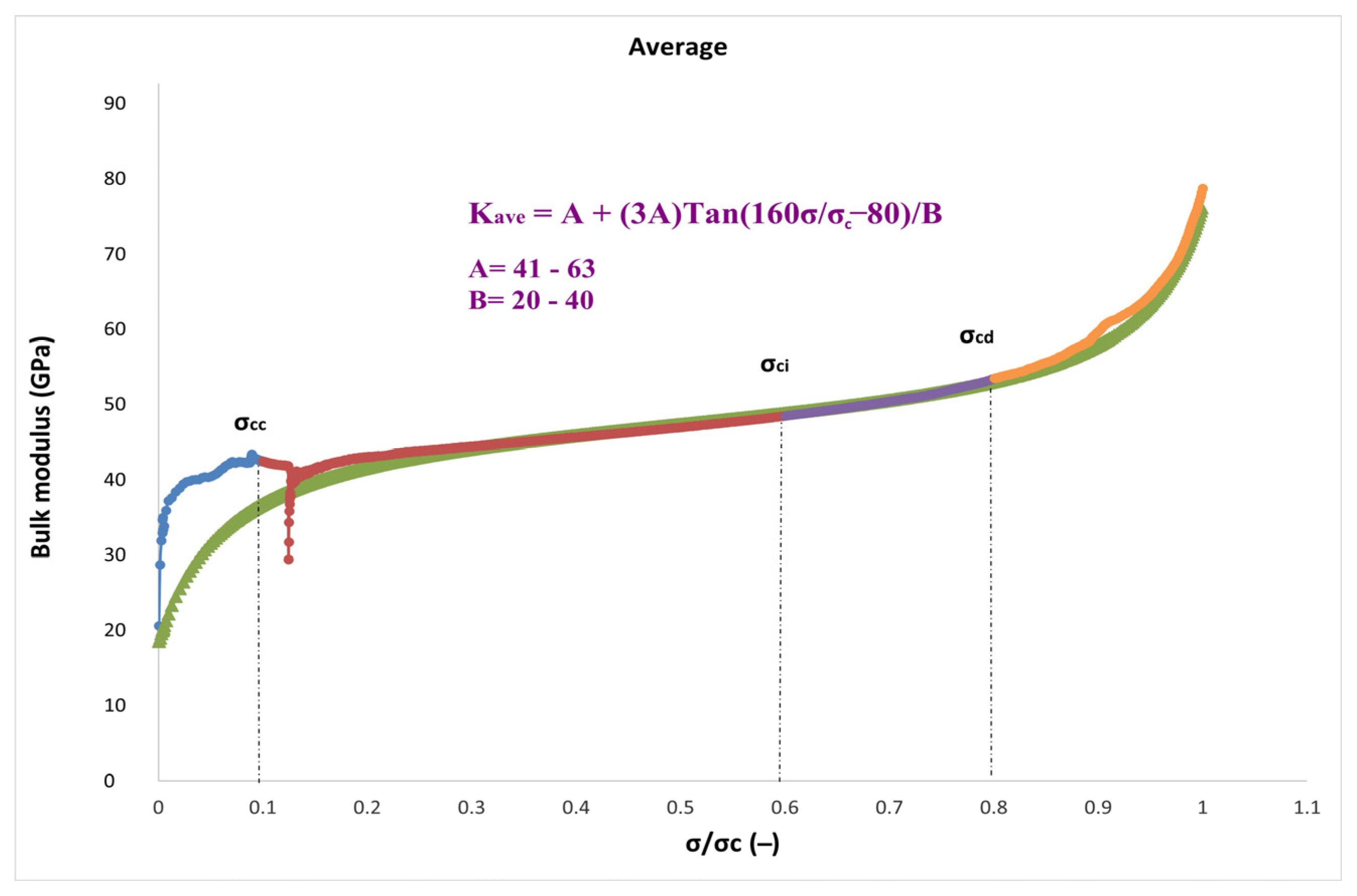
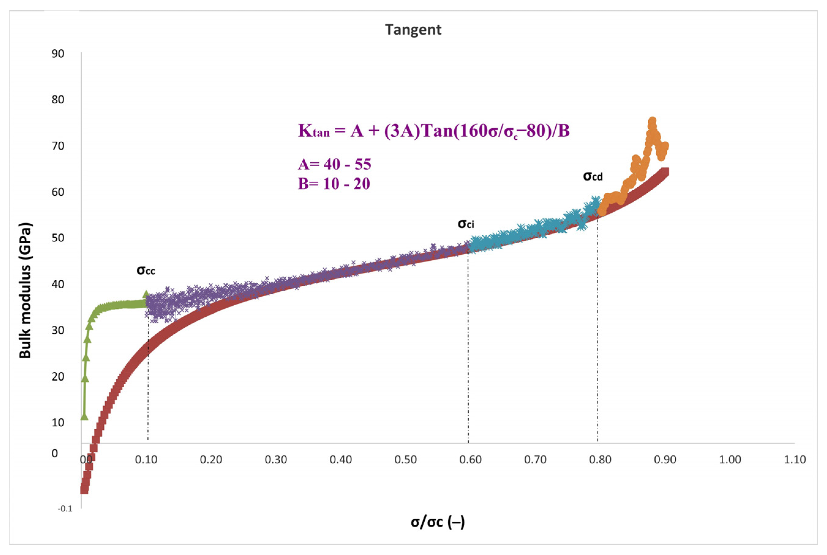
The bulk modulus at σ/σc = 0.5, which is denoted by constant A, is referred to as K0.5 in the equation. Degree is defined as 160σ/σc−80 in terms of tan(degree), where tan90 is infinite. B is constant and depends on the type of rock. Hence, the following equation will represent the final bulk modulus calculation:
K = A + 3A tan(160σ/σc−80)/B
In three separate scenarios—secant, average, and tangent—the novel suggested model was used to calculate the bulk modulus with constants A and B obtained for each case. Table 3 provides a summary of the findings.
The variations of the bulk modulus for the secant, average, and tangent cases are shown in Figure 5, Figure 6 and Figure 7. In contrast to the secant and average functions, the slope of the bulk modulus variations in the tangent functions is more intense, as illustrated in the figures. The range of crack closure via crack damage stress stages is where the suggested model’s best fit to experimental data is found, in accordance with the data. In addition, between the crack closure and crack damage stages of the loading process, the secant and average bulk modulus develop roughly linearly with stress variations.
Compared to the Young’s and shear moduli, the general behavior of the bulk modulus is quite different. In other words, while the Young’s and shear moduli illustrate nonlinear parabolic function, which starts to decrease after 50% of σ/σc, the bulk modulus follows increasing nonlinear function from the beginning of loading through the failure state. The reason is more likely connected with the effect of the Poisson’s ratio. In other words, the bulk modulus is more influenced by the Poisson’s ratio.
2.3. Regression Analysis between E, G, and K in Three Diferent Scenarios
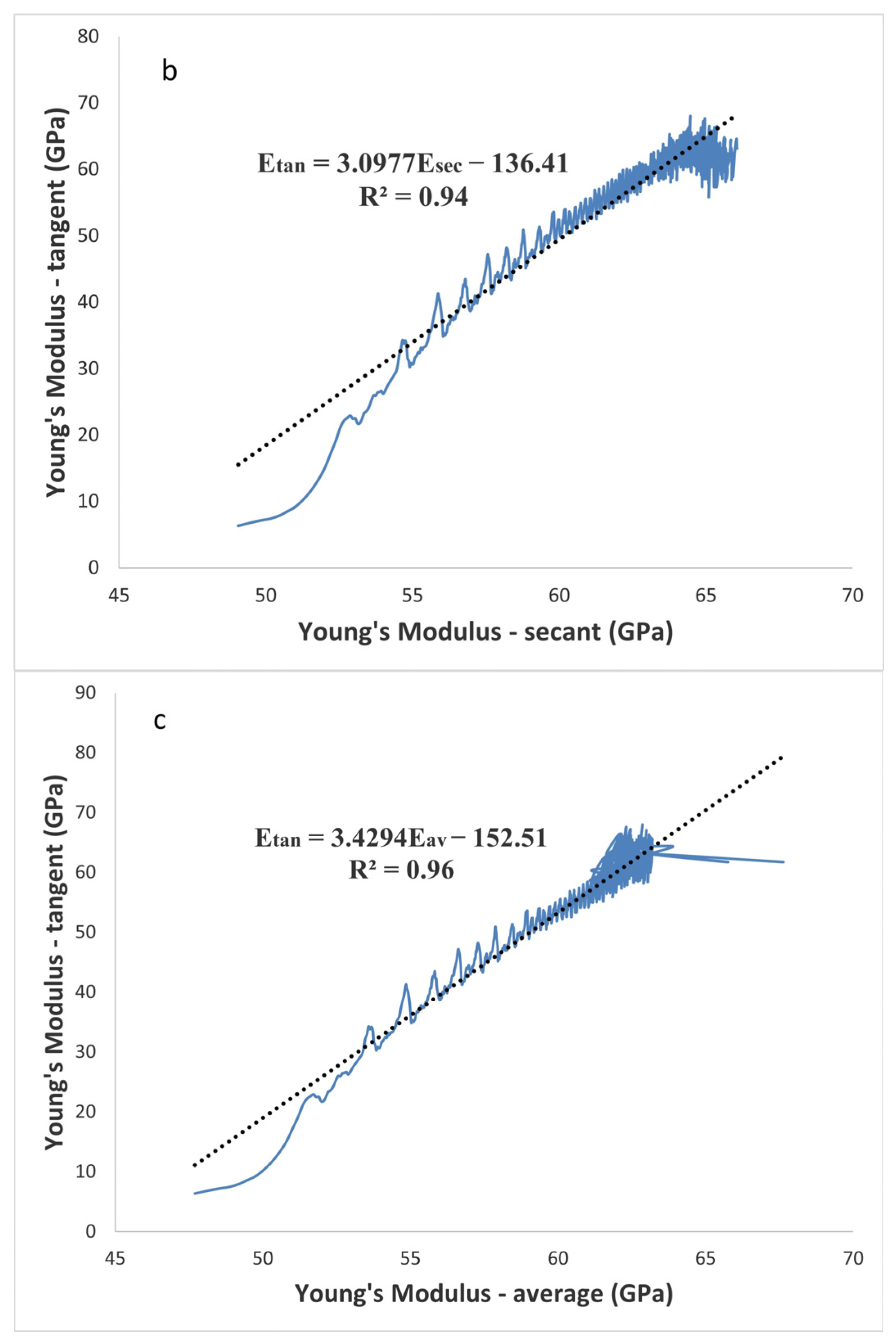
Our research (Figure 8) shows that there have recently been published studies of linear connections between the Young’s modulus constants. Figure 8 illustrates the average Young’s modulus and tangent values, which have an R2 value of 0.96 and are significantly connected linearly. Although both the tangent and average Young’s modulus and the tangent and secant Young’s modulus have R2 values of 0.94, trends can also be traced linearly between these two Young’s moduli. Moreover, according to Figure 8b, the data scattering is denser from 60% of σ/σc through the failure, and it can be related to growing the network of cracks under loading in the uniaxial compressive strength (UCS) test. However, data scattering is less dense from the beginning to 60% of σ/σc, as the crack network is still not widely distributed.
In other words, as a result of the shear modulus-focused analysis shown in Figure 9, the achieved correlations for all situations are also linear with the highest regression coefficient associated with the secant and the average shear modulus with an R2 value of 0.99. Similar to this, there was a strong association between the secant and average shear modulus (R2 = 0.9) and the tangent and average shear modulus (R2 = 0.94) (Figure 9b,c). In addition, Figure 9b,c shows that the data dispersion is more dense from 60% of σ/σc through the failure, which is possibly connected to the expansion of the network of fractures during the uniaxial compressive strength (UCS) test. Due to the fracture network’s lack of widespread distribution, data scattering is less dense from the beginning to 60% of σ/σc.
In Figure 10a, the linear relationship between the secant and average bulk modulus is shown. At R2 = 0.99, it exhibits a strong correlation. The correlation is, nevertheless, significantly reduced in Figure 10b,c when we compute the secant and tangent bulk modulus and the average and tangent bulk modulus, respectively. Figure 10b,c shows that there is not a particularly strong correlation between the secant and tangent bulk modulus (R2 = 0.6) or the tangent and average bulk modulus (R2 = 0.57), and that both of these have nonlinear and exponential patterns.
The proposed equations have a strong prediction capacity and can be used to estimate the Young’s modulus (E), shear modulus (G), and bulk modulus (K) of intact granitic rocks for practical purpose.
3. Discussion
The basic idea behind the current research is the statement of a new method to estimate the elastic stiffness properties (E, G, and K) of intact granitic rocks. For this objective, samples were supplied from the Bataapáti radioactive waste repository of Hungary.
The Young’s modulus is equal to the ratio of stress to strain, as stated in Equation (2). Yet, treating the Young’s modulus as an elastic constant is a dubious practice because the Young’s modulus of a rock varies continuously, even during the linear elastic stage. Because the crack propagation threshold can vary, the amount of the Young’s modulus can have a big impact on how progressive failure processes are broken down into stages.
Unaffected by the approach, variations in E, G, and K for granitic rocks for the UCS test are investigated. This is one of the important findings from the evaluation presented in this paper. The common theory that the amounts of E, G, and K in rocks are constant is refuted by these discoveries. Our findings show that, even though the established equation for estimating the bulk modulus follows nonlinear and tangential function, the representative equations for calculating the change of the Young’s modulus and shear modulus are nonlinear and follow parabolic function.
The Young’s modulus, shear modulus, and bulk modulus all react very differently when granitic rocks are subjected to uniaxial compression, as we discovered by studying the deformation mechanisms of these rocks. The shear modulus and Young’s modulus have behavior that is remarkably comparable and follow parabolic curves. The proposed equations for E and G have variable constants based on the granitic rock under investigation. On the other hand, since the secant, average, and tangent bulk moduli rise monotonically with increasing stress, there is no plateau in the bulk modulus diagrams. This tendency might be connected to the propagation of microcracks and the irreversibility of compaction in the direction of compression.
Also, we were able to achieve correlations for the three variables E, G, and K with strong determination factors in secant, tangent, and average scenarios. One limitation of this experiment was the lack of variety in the kinds of rock. These prediction equations can be used in additional studies to predict E, G, and K using a variety of rock types more precisely. The aforementioned predictive equations can, therefore, be utilized to forecast the stiffness properties of rock depending on the circumstance.
Our findings are unlikely to be generalizable due to the vast variety of rocks in the world, each of which has unique features, as well as the small number of specimens used in this study. The behavior of elastic stiffness parameters in rocks needs to be understood thoroughly and in-depth, which will require many more empirical studies.
The deformation behavior of intact rock is mainly controlled by the development of crack networks. Considering this fact, the propagation of cracks in each step of the UCS test can be applied with corresponding stiffness behavior.
The future work can be directed to study the effect of confining pressure of the intact rock in the variation of elastic stiffness parameters in the triaxial test. Moreover, the Poisson’s ratio has a significant impact on the mechanical behavior of intact rock. So, it is necessary to investigate the variation of the Poisson’s ratio in the UCS test.
4. Conclusions
This research work proposes a new idea to calculate the elastic stiffness parameter, including the Young’s modulus, shear modulus, and bulk modulus of granitic intact rock from the crack closure through the failure stage. According to our findings, all the moduli parameters do not follow linear function. In other words, the Young’s modulus and shear modulus follow nonlinear parabolic equations with a different material constant for the three different scenarios: secant, tangent, and average. Moreover, the bulk modulus of the investigated samples indicates different behavior than the Young’s and shear moduli, as it is more dependent on the Poisson’s ratio behavior of the rock. So, our study leads to the new equations, which provide a good estimation of the bulk modulus during the loading in the UCS test in three different cases: secant, tangent, and average.
Strong and consistent correlations were observed for the Young’s modulus and shear modulus between secant-tangent, secant-average, and average-tangent. However, the correlation achieved for the bulk modulus was not considerable between secant-tangent (R2 = 0.6) and average-tangent (R2 = 0.57), similar to the previous research. Furthermore, considering the relationship between secant and average for all the elastic stiffness moduli is linear with a high coefficient of determination. Otherwise, as is the case of tangent correlation with secant and average, a nonlinear trend is observed, and data scattering is wider.
Finally, we stress that the approach presented herein is by no means complete. We now need more laboratory data and a more effective way to account for elastic stiffness moduli.
Author Contributions
S.N.: structure and writing, S.M.D.: calculation, L.K.: processing and calculation, B.V.: methodology. All authors have read and agreed to the published version of the manuscript.
Funding
This research received no external funding.
Institutional Review Board Statement
Not applicable.
Informed Consent Statement
Not applicable.
Data Availability Statement
Not applicable.
Conflicts of Interest
The authors declare no conflict of interest.
References
- Xiong, L.X.; Xu, Z.Y.; Li, T.B.; Zhang, Y. Bonded-particle discrete element modeling of mechanical behaviors of interlayered rock mass under loading and unloading conditions. Geomech. Geophys. Geo-Energy Geo-Resour. 2019, 5, 1–16. [Google Scholar] [CrossRef]
- Yang, J.; Hatcherian, J.; Hackley, P.C.; Pomerantz, A.E. Nanoscale geochemical and geomechanical characterization of organic matter in shale. Nat. Commun. 2017, 8, 2179. [Google Scholar] [CrossRef] [Green Version]
- Zhao, Y.S.; Wan, Z.J.; Feng, Z.J.; Xu, Z.H.; Liang, W.G. Evolution of mechanical properties of granite at high temperature and high pressure. Geomech. Geophys. Geo-Energy Geo-Resour. 2017, 3, 199–210. [Google Scholar] [CrossRef]
- Ranjith, P.G.; Fourar, M.; Pong, S.F.; Chian, W.; Haque, A. Characterisation of fractured rocks under uniaxial loading states. Int. J. Rock Mech. Min. Sci. 2004, 41, 361–366. [Google Scholar] [CrossRef]
- Rahimi, R.; Nygaard, R. Effect of rock strength variation on the estimated borehole breakout using shear failure criteria. Geomech. Geophys. Geo-Energy Geo-Resour. 2018, 4, 369–382. [Google Scholar] [CrossRef]
- Davarpanah, M.; Somodi, G.; Kovács, L.; Vásárhelyi, B. Complex analysis of uniaxial compressive tests of the Mórágy granitic rock formation (Hungary). Stud. Geotech. Mech. 2019, 41, 21–32. [Google Scholar] [CrossRef] [Green Version]
- Davarpanah, S.M.; Bar, N.; Török, Á.; Tarifard, A.; Vásárhelyi, B. Technical Note: Determination of Young’s Modulus and Poisson’s Ratio for Intact Stratified Rocks and Their Relationship with Uniaxial Compressive Strength. Aust. Geomech. J. 2020, 55, 101–118. [Google Scholar]
- Tsang, L.; He, B.; Rashid, A.S.; Jalil, A.T.; Sabri, M.M. Predicting the Young’s Modulus of Rock Material Based on Petrographic and Rock Index Tests Using Boosting and Bagging Intelligence Techniques. Appl. Sci. J. 2022, 12, 10258. [Google Scholar] [CrossRef]
- Bieniawski, Z.T. Stability concept of brittle fracture propagation in rock. Eng. Geol. 1967, 2, 149–162. [Google Scholar] [CrossRef]
- Brady, B.H.G.; Brown, E.T. Rock Mechanics for Underground Mining, 3rd ed.; Springer: London, UK, 2006. [Google Scholar]
- ISRMRE. Suggested methods for determining the uniaxial compressive strength and deformability of rock materials. Int. J. Rock Mech. Min. Sci. Geomech. Abstr. 1978, 16, 135–140. [Google Scholar] [CrossRef]
- Ulusay, R.; Hudson, J.A. The Blue Book: “The Complete ISRMRE Suggested Methods for Rock Characterization, Testing and Monitoring: 1974-2006”; ISRMRE Turkish National Group: Ankara, Turkey, 2007. [Google Scholar]
- Malik, M.H.; Rashid, S. Correlation of Some Engineering Geological Properties of the Murree Formation at Lower Topa (Murree District), Pakistan. Geol. Bull. Univ. Peshawar 1997, 30, 69–81. [Google Scholar]
- Martin, C.D.; Chandler, N.A. The progressive fracture of Lac du Bonnet granite. Int. J. Rock Mech. Min. Sci. Geomech. Abstr. 1994, 6, 643–659. [Google Scholar] [CrossRef]
- Ulusay, R. Rock Properties and Their Role in Rock Characterization, Modelling and Design; ISRMRE: Ankara, Turkey, 2018. [Google Scholar]
- Davarpanah, M.; Somodi, G.; Kovács, L.; Vásárhelyi, B. Experimental determination of the mechanical properties and deformation constants of Mórágy granitic rock formation (Hungary). Geotech. Geol. Eng. 2020, 38, 3215–3229. [Google Scholar] [CrossRef] [Green Version]
- Blake, O.O.; Faulkner, D.R.; Tatham, D.J. The role of fractures, effective pressure and loading on the difference between the static and dynamic Poisson’s ratio and Young’s modulus of Westerly granite. Int. J. Rock Mech. Mining Sci. 2019, 116, 87–98. [Google Scholar] [CrossRef]
- Martínez-Martínez, J.; Benavente, D.; García-del-Cura, M.A. Comparison of the static and dynamic elastic modulus in carbonate rocks. Bull. Eng. Geol. Environ. 2012, 71, 263–268. [Google Scholar] [CrossRef]
- Nguyen, V.; Abousleiman, Y.; Hoang, S. Analyses of wellbore instability in drilling through chemically active fractured-rock formations. SPE. J. 2009, 14, 283–301. [Google Scholar] [CrossRef]
- William, L.F. The Variation of Young’s Modulus with Rock Type and Temperature. Master’s Thesis, University of Wisconsin, Madison, WI, USA, 1969. Available online: https://www.yumpu.com/en/document/view/5492718/rock-properties-and-their-role-in-rock-characterization-isrm (accessed on 6 March 2023).
- Davarpanah, M.; Török, A.; Vásárhelyi, B. Review on the mechanical properties of frozen rocks. Rud. Geološko-Naft. Zb. 2022, 37, 83–96. [Google Scholar] [CrossRef]
- Santi, P.M.; Holschen, J.E.; Stephenson, R.W. Improving Elastic Modulus Measurements for Rock Based on Geology. Environ. Eng. Geosci. 2000, 4, 333–346. [Google Scholar] [CrossRef]
- Malkowski, P.; Ostrowski, L.; Brodny, J. Analysis of Young’s modulus for Carboniferous sedimentary rocks and its relationship with uniaxial compressive strength using different methods of modulus determination. J. Sustain. Min. 2018, 17, 145–157. [Google Scholar] [CrossRef]
- Briševac, Z.; Pollak, D.; Maričić, A.; Vlahek, A. Modulus of Elasticity for Grain-Supported Carbonates—Determination and Estimation for Preliminary Engineering Purposes. Appl. Sci. 2021, 11, 6148. [Google Scholar] [CrossRef]
- Madhubabu, N.; Singh, P.K.; Kainthola, A.; Mahanta, B.; Tripathy, A.; Singh, T.N. Prediction of compressive strength and elastic modulus of carbonate rocks. Measurement 2016, 88, 202–213. [Google Scholar] [CrossRef]
- Palchik, V.; Hatzor, Y.H. Crack damage stress as a composite function of porosity and elastic matrix stiffness in dolomites and limestones. Eng. Geol. 2002, 63, 233–245. [Google Scholar] [CrossRef]
- Pells, P.J.N. Unixial Strength Testing. In Comprehensive Rock Engineering: Principles, Practice and Projects; Hudson, J.A., Ed.; Pergamon Press: Oxford, UK, 1993; Volume 3, pp. 67–85. [Google Scholar]
- Rybacki, E.; Reinicke, A.; Meier, T.; Makasi, M.; Dresen, G. What controls the mechanical properties of shale rocks?—Part I: Strength and Young’s modulus. J. Pet. Sci. Eng. 2015, 135, 702–722. [Google Scholar] [CrossRef]
- Sabatakakis, N.; Koukis, G.; Tsiambaos, G.; Papanakli, S. Index properties and strength variation controlled by microstructure for sedimentary rocks. Eng. Geol. 2008, 97, 80–90. [Google Scholar] [CrossRef]
Figure 1.
Schematic calculation of (a) secant Poisson’s ratio (νs), tangent Poisson’s ratio (νt), and average Poisson’s ratio (νav); (b) secant Young’s Modulus (Es), tangent Young’s Modulus (Et), and average Young’s Modulus (Eav).
Figure 1.
Schematic calculation of (a) secant Poisson’s ratio (νs), tangent Poisson’s ratio (νt), and average Poisson’s ratio (νav); (b) secant Young’s Modulus (Es), tangent Young’s Modulus (Et), and average Young’s Modulus (Eav).

Figure 2.
A common stress–strain diagram for rock showing axial, transverse, and volumetric deformation [13].
Figure 2.
A common stress–strain diagram for rock showing axial, transverse, and volumetric deformation [13].

Figure 3.
A typical secant, tangent, and average Young’s modulus-σ/σc curve for granitic specimens.

Figure 4.
A typical secant, tangent, and average shear modulus-σ/σc curve for granitic specimens.

Figure 5.
A typical secant bulk modulus-σ/σc curve for granitic specimens. The colored lines are for separating the stages of the loading. Blue is for crack closure part. Red is for crack initiation part. Dark blue is for crack damage part. And orange is for the final failure part.
Figure 5.
A typical secant bulk modulus-σ/σc curve for granitic specimens. The colored lines are for separating the stages of the loading. Blue is for crack closure part. Red is for crack initiation part. Dark blue is for crack damage part. And orange is for the final failure part.

Figure 6.
A typical average bulk modulus-σ/σc curve for granitic specimens. The colored lines are for separating the stages of the loading. Blue is for crack closure part. Red is for crack initiation part. Dark blue is for crack damage part. And orange is for the final failure part.
Figure 6.
A typical average bulk modulus-σ/σc curve for granitic specimens. The colored lines are for separating the stages of the loading. Blue is for crack closure part. Red is for crack initiation part. Dark blue is for crack damage part. And orange is for the final failure part.

Figure 7.
A typical tangent bulk modulus-σ/σc curve for granitic specimens. The colored lines are for separating the stages of the loading. Blue is for crack closure part. Red is for crack initiation part. Dark blue is for crack damage part. And orange is for the final failure part.
Figure 7.
A typical tangent bulk modulus-σ/σc curve for granitic specimens. The colored lines are for separating the stages of the loading. Blue is for crack closure part. Red is for crack initiation part. Dark blue is for crack damage part. And orange is for the final failure part.

Figure 8.
Relationship between (a) Eave-Esec, (b) Etan-Esec, and (c) Etan-Eave.


Figure 9.
Relationship between (a) Gave-Gsec, (b) Gtan-Gsec, and (c) Gtan-Gave.

Figure 10.
Relationship between (a) Kave-Ksec, (b) Ktan-Ksec, and (c) Ktan-Kave.


Table 1.
Equations and related constants for the Young’s modulus in different cases.
| Young’s Modulus | Equation | Constant a | Constant b | Constant c |
|---|---|---|---|---|
| Secant | Esec = ax2 + bx + c | −10 to −19 | 9 to 19 | 65 to 75 |
| Average | Eave = ax2 + bx + c | −14 to −24 | 9 to 18 | 61 to 76 |
| Tangent | Etan = ax2 + bx + c | −22 to −67 | 18 to 36 | 59 to 77 |
Table 2.
Equations and related constants for the shear modulus in different cases.
| Shear Modulus | Equation | Constant a | Constant b | Constant c |
|---|---|---|---|---|
| Secant | Gsec = ax2 + bx + c | −5 to −15 | 3 to 14 | 21 to 30 |
| Average | Gav = ax2 + bx + c | −4 to −14 | 2 to 13 | 25 to 32 |
| Tangent | Gtan = ax2 + bx + c | −20 to −45 | 8 to 30 | 22 to 31 |
Table 3.
Equations and related constants for the bulk modulus in different cases.
| Bulk Modulus | Equation | Constant A | Constant B |
|---|---|---|---|
| Secant | Ksec = A + (3A) tan(160σ/σc−80)/B | 36 to 55 | 20 to 40 |
| Average | Kav = A + (3A) tan(160σ/σc−80)/B | 41 to 62 | 20 to 40 |
| Tangent | Ktan = A + (3A) tan(160σ/σc−80)/B | 40 to 55 | 10 to 20 |
Disclaimer/Publisher’s Note: The statements, opinions and data contained in all publications are solely those of the individual author(s) and contributor(s) and not of MDPI and/or the editor(s). MDPI and/or the editor(s) disclaim responsibility for any injury to people or property resulting from any ideas, methods, instructions or products referred to in the content. |
© 2023 by the authors. Licensee MDPI, Basel, Switzerland. This article is an open access article distributed under the terms and conditions of the Creative Commons Attribution (CC BY) license (https://creativecommons.org/licenses/by/4.0/).
Share and Cite
MDPI and ACS Style
Narimani, S.; Davarpanah, S.M.; Kovács, L.; Vásárhelyi, B. Variation of Elastic Stiffness Parameters of Granitic Rock during Loading in Uniaxial Compressive Test. Appl. Mech. 2023, 4, 445-459. https://doi.org/10.3390/applmech4020025
AMA Style
Narimani S, Davarpanah SM, Kovács L, Vásárhelyi B. Variation of Elastic Stiffness Parameters of Granitic Rock during Loading in Uniaxial Compressive Test. Applied Mechanics. 2023; 4(2):445-459. https://doi.org/10.3390/applmech4020025
Chicago/Turabian StyleNarimani, Samad, Seyed Morteza Davarpanah, László Kovács, and Balázs Vásárhelyi. 2023. "Variation of Elastic Stiffness Parameters of Granitic Rock during Loading in Uniaxial Compressive Test" Applied Mechanics 4, no. 2: 445-459. https://doi.org/10.3390/applmech4020025