Article

Data-Driven, Physics-Based, or Both: Fatigue Prediction of Structural Adhesive Joints by Artificial Intelligence

by
Pedro Henrique Evangelista Fernandes
1,2,
Giovanni Corsetti Silva
3,
Diogo Berta Pitz
4,
Matteo Schnelle
1,
Katharina Koschek
1,
Christof Nagel
1 and
Vinicius Carrillo Beber
1,*
1
Fraunhofer Institute for Manufacturing Technology and Advanced Materials IFAM, 28359 Bremen, Germany
2
Faculty 4—Production Engineering, University of Bremen, 28359 Bremen, Germany
3
Department of Mechanical Engineering, Federal University of Paraná, Curitiba 81531-980, PR, Brazil
4
Postgraduate Program of Mechanical Engineering—PGMEC, Federal University of Paraná, Curitiba 81531-980, PR, Brazil
*
Author to whom correspondence should be addressed.
Appl. Mech. 2023, 4(1), 334-355; https://doi.org/10.3390/applmech4010019
Submission received: 5 February 2023 / Revised: 24 February 2023 / Accepted: 6 March 2023 / Published: 8 March 2023
(This article belongs to the Special Issue Feature Papers in Applied Mechanics)

Abstract

:
Here, a comparative investigation of data-driven, physics-based, and hybrid models for the fatigue lifetime prediction of structural adhesive joints in terms of complexity of implementation, sensitivity to data size, and prediction accuracy is presented. Four data-driven models (DDM) are constructed using extremely randomized trees (ERT), eXtreme gradient boosting (XGB), LightGBM (LGBM) and histogram-based gradient boosting (HGB). The physics-based model (PBM) relies on the Findley’s critical plane approach. Two hybrid models (HM) were developed by combining data-driven and physics-based approaches obtained from invariant stresses (HM-I) and Findley’s stress (HM-F). A fatigue dataset of 979 data points of four structural adhesives is employed. To assess the sensitivity to data size, the dataset is split into three train/test ratios, namely 70%/30%, 50%/50%, and 30%/70%. Results revealed that DDMs are more accurate, but more sensitive to dataset size compared to the PBM. Among different regressors, the LGBM presented the best performance in terms of accuracy and generalization power. HMs increased the accuracy of predictions, whilst reducing the sensitivity to data size. The HM-I demonstrated that datasets from different sources can be utilized to improve predictions (especially with small datasets). Finally, the HM-I showed the highest accuracy with an improved sensitivity to data size.

1. Introduction

Structural adhesives, as polymeric materials, tend to overheat at extreme frequencies, which makes fatigue testing highly time- and cost-consuming. For instance, a fatigue test with 10 million cycles at a frequency of 10 Hz would last approximately 11.6 days. Considering that several data points are required for the construction of a fatigue design curve (SN curve), the development of approaches to take advantage of existing datasets can be very beneficial.
Structural adhesive joining is widely regarded as a key technology for the development of reliable lightweight components by using multi-material design and efficient load distribution. These capabilities can enable the reduction of production costs, as well as improve energy efficiency [1,2]. Concerning durability and long-term behavior, the fatigue has a great impact on the design of adhesively bonded joints, as cyclic loads are commonly present during their lifetime [3]. An additional challenge is that adhesive joints have a particularity: they are not made of a single material, but from at least an adhesive (a polymer), and two substrates (metal, polymer, or composite).
A suitable design against fatigue should include all factors that might influence on the fatigue lifetime in order to depict the expected in-service conditions of structural adhesive joints [4]. However, many factors have an effect on the fatigue strength of structural adhesives, such as mean stress [5,6,7], stress concentrations [8,9], stress multiaxiality [7,10], temperature [11,12,13,14], non-proportional loading [6,15], and others. Therefore, in order to cover all of these aspects, an extensive experimental campaign is expected.
An interesting approach to deal with such complex phenomena (e.g., fatigue) is to take advantage of the existing available data. In this context, artificial intelligence (AI) is known for its capacity to solve large-scale problems by learning from previous knowledge, enabling the generation of quantitative expressions that successfully represent complex relationships between parameters [16].
However, a shortcoming of data-driven AI approaches in the framework of materials science is associated with the limited availability of data and the difficulty to generate large data sizes. Although initiatives (e.g., DOME4.0 [17] and NFDI MatWerk [18]) have been developed in recent years to create repositories and marketplaces for materials science and engineering data, the access to data is still restricted. In this regard, modeling the fatigue lifetime of structural adhesive joints can be challenging due to the constraints posed by small datasets. One solution to this issue is to integrate heterogeneous data sources. As such, AI-based data-driven models can incorporate fatigue data from various sources, such as peer-reviewed articles, reports, and material databases, by exploiting the similarities in behavior among materials within the same category [19].
In tasks involving small datasets, domain knowledge is crucial in choosing the most relevant features and avoiding overfitting in modeling. Overfitting occurs when a model is too closely tailored to the training data and struggles to properly generalize when exposed to new data [20]. The feature engineering process may uncover complex relationships between inputs, leading to a simpler model with reduced parameters. This domain knowledge can be introduced by informing AI-models of existing correlations between parameters, which are backed by physics-based relationships. Approaches such as the physics-informed neural networks (PINNs)—with the motto “big data, small physics—small data, big physics”—can significantly improve the prediction capability of AI-models [21,22,23].
A consequence of the use of smaller datasets is that shallow learning algorithms, such as decision trees and shallow neural networks, tend to perform better than deep learning algorithms [24]. This is because deep learning algorithms bring in more complexity and require a substantial amount of data to fine-tune a model. Therefore, it is important to consider both the task at hand and the size of the dataset when selecting an ML algorithm [25]. Addressing the modeling of adhesive joints for small datasets, Zhu et al. [26] used back-propagation (BP) neural network to model the accelerated degradation of epoxy resin. Mansouri et al. [27] were able to predict the compressive strength of environmentally friendly concrete using hybrid ML based on 147 datasets. For fatigue applications, Zhou et al. [28] employed 27 specimens to identify genetic features and to predict the fatigue lifetime of stainless steel. Heng et al. [29] employed FEA to generate data for the training of a surrogate model for probabilistic fatigue evaluation of rib-to-deck joints.
Therefore, considering the task of lifetime predictoin of structural adhesive joints, prediction models should ideally be accurate, interpretable, computationally efficient, generalizable, and able to perform with reduced datasets [30]. In this regard, three approaches can be taken into consideration: physics-based models (PBM), data-driven models (DDM), and a third is the development of hybrid models (HM), which combine both data-driven and physics-based characteristics.
Physics-based models relying on the stress-life criteria can be considered the state-of-the-art for fatigue lifetime prediction of adhesively bonded joints [3]. Among them, invariant stress criteria have been widely used [10,12,31,32] with suitable accuracy. Recently, especially in cases under non-proportional loading (i.e., with phase-shift), critical plane stress criteria are gaining more attraction in fatigue applications (e.g., Beber et al. [33], Fernandes et al. [15], and Beugre et al. [34]). However, a common limitation of physics-based approaches is that parameters are adhesive-dependent, i.e., for each new adhesive the parameters for lifetime prediction have to be calibrated.
Regarding data-driven-models, there is a rising trend on the usage of DDM for lifetime predictions [35]. Several authors have investigated the implementation of AI-based methods [21,23,35,36] for lifetime predictions in materials science. More specifically, for the fatigue of adhesive joints, Sekercioglu and Kovan [37] used ANN to predict the fatigue lifetime of adhesively bonded cylindrical joints. Silva et al. [38] proposed an integrated approach combining ML (an ERT-model) and finite element analysis to predict the fatigue lifetime of adhesively bonded joints. Other authors have employed ML approaches for the static strength of structural adhesive joints, e.g., Schubert and Kläusler [39], Pruksawan et al. [40], and Gajewski et al. [41].
For hybrid models, Chen and Liu employed a physics-guided machine learning approach for fatigue data analysis of metals and composite materials. He et al. [42] developed a physics-informed neural network based on the critical plane approach to predict the multiaxial fatigue lifetime of three different materials. Shutin et al. [43] combined DDM and PBM to predict the useful life of metallic load bearings. Nonetheless, the field of hybrid approaches combining data-driven and physics-based methods for fatigue modeling of structural adhesive joints is, to our knowledge, still very scarce.
In this scenario, the current work presents a comparative investigation of data-driven, physics-based, and hybrid models for the fatigue lifetime prediction of structural adhesive joints. The different modeling approaches are compared in terms of complexity of implementation, sensitivity to data size, and prediction accuracy. Four data-driven models are constructed using different regressors, namely extremely randomized trees, eXtreme gradient boosting, LightGBM, and histogram-based gradient boosting. The physics-based model employs the critical plane approach. Then, two hybrid models are developed by combining data-driven approaches with physics-based parameters obtained from the (i) invariant stresses and (ii) the critical plane stress.
The fatigue dataset consists of 979 fatigue data points from four structural adhesives with four joint configurations taken from heterogeneous data sources. To assess the sensitivity to data size, the fatigue dataset is split with three different ratios of the train/test dataset, namely 70%/30%, 50%/50%, and 30%/70%. Prediction accuracy is evaluated by the R2, as well as the error factor (ER) for lifetime predictions of the train and test datasets.

2. Fatigue Dataset

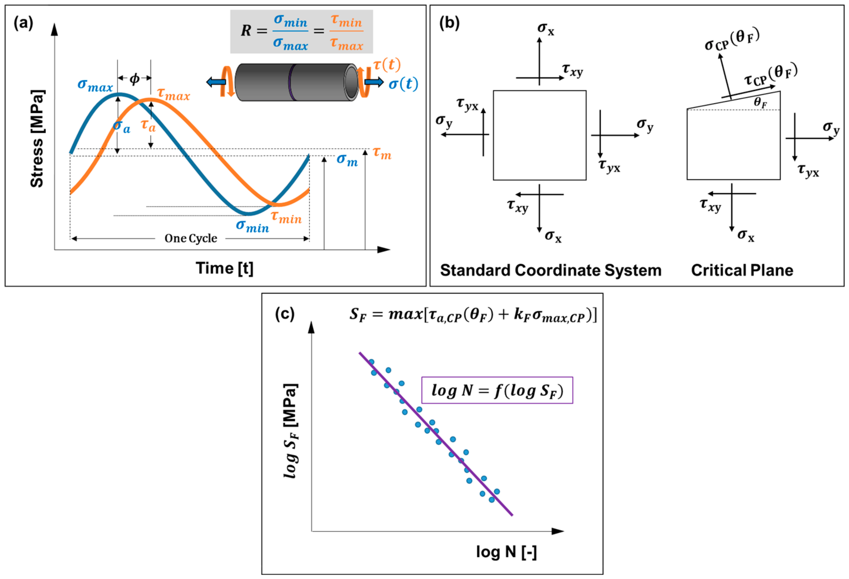
2.1. Fatigue Loading Parameters

For a constant amplitude fatigue loading under sinusoidal shape, the value of the shear stress τ t and tensile stress σ t , at any time, can be obtained as a function of the mean shear stress τ m and the shear stress amplitude τ a , as well as the mean tensile stress σ m and the tensile stress amplitude σ a :
τ t = τ m + τ a sin 2 π f t + ϕ τ π 180
σ t = σ m + σ a sin 2 π f t + ϕ σ π 180
where t is the time in [s], f is the frequency in [Hz], ϕ τ ,   and ϕ σ are the phase-shift for shear and tensile stresses, respectively, in [°]. The relative phase-shift ϕ between the shear and tensile stresses is defined in [°] as:
ϕ = ϕ τ ϕ σ
The stress amplitude can be written as a function of the maximum ( σ m a x   or   τ m a x ) and minimum stress ( σ m i n   or   τ m i n ) of the cyclical load:
σ a = σ m a x σ m i n 2   or   τ a = τ m a x τ m i n 2  
The stress ratio R is defined as follows:
R = σ m i n σ m a x = τ m i n τ m a x
Based on the stress amplitude, R can be a measure of the intensity of the mean stress:
σ m = 1 + R 1 R σ a   or   τ m = 1 + R 1 R τ a
The fatigue loading parameters are graphically represented in Figure 1a considering a phase-shifted multiaxial stress state with shear and tensile stresses.

2.2. Dataset Description

The fatigue dataset employed in the current investigation was mined from publicly accessible scientific literature [5,6,7,14,15,33,44,45]. The dataset consists of 979 fatigue data points measured at room temperature from four different structural adhesives. As this information was not clearly stated in every publication, we have assumed a cohesive failure of the adhesive layer (i.e., ideal adhesion between substrates and the adhesive).
As shown in Table 1, seven publications were collected to construct the fatigue dataset. Additionally, parameters related to both the adhesive and the substrates are listed: ultimate tensile strength of the adhesive ( U T S a d ), Young’s modulus of the adhesive ( E a d ), Poisson’s ratio of the adhesive ( ν a d ), Young’s modulus of the substrate ( E s u b ), and Poisson’s ratio of the substrate ( ν s u b ).
Due to availability, the amount of data per adhesive is not totally balanced, e.g., the adhesive Ad1 makes 58.5% of the total amount. The consideration of multiple structural adhesives in the dataset helps to evaluate the fatigue prediction capability of the model to integrate heterogeneous data sources.
A statistical analysis of the fatigue dataset is presented in Table 2, where the central tendency, dispersion, and shape can be seen. The parameters listed here (see Figure 1a) will be used for the implementation of the models (see Section 3).

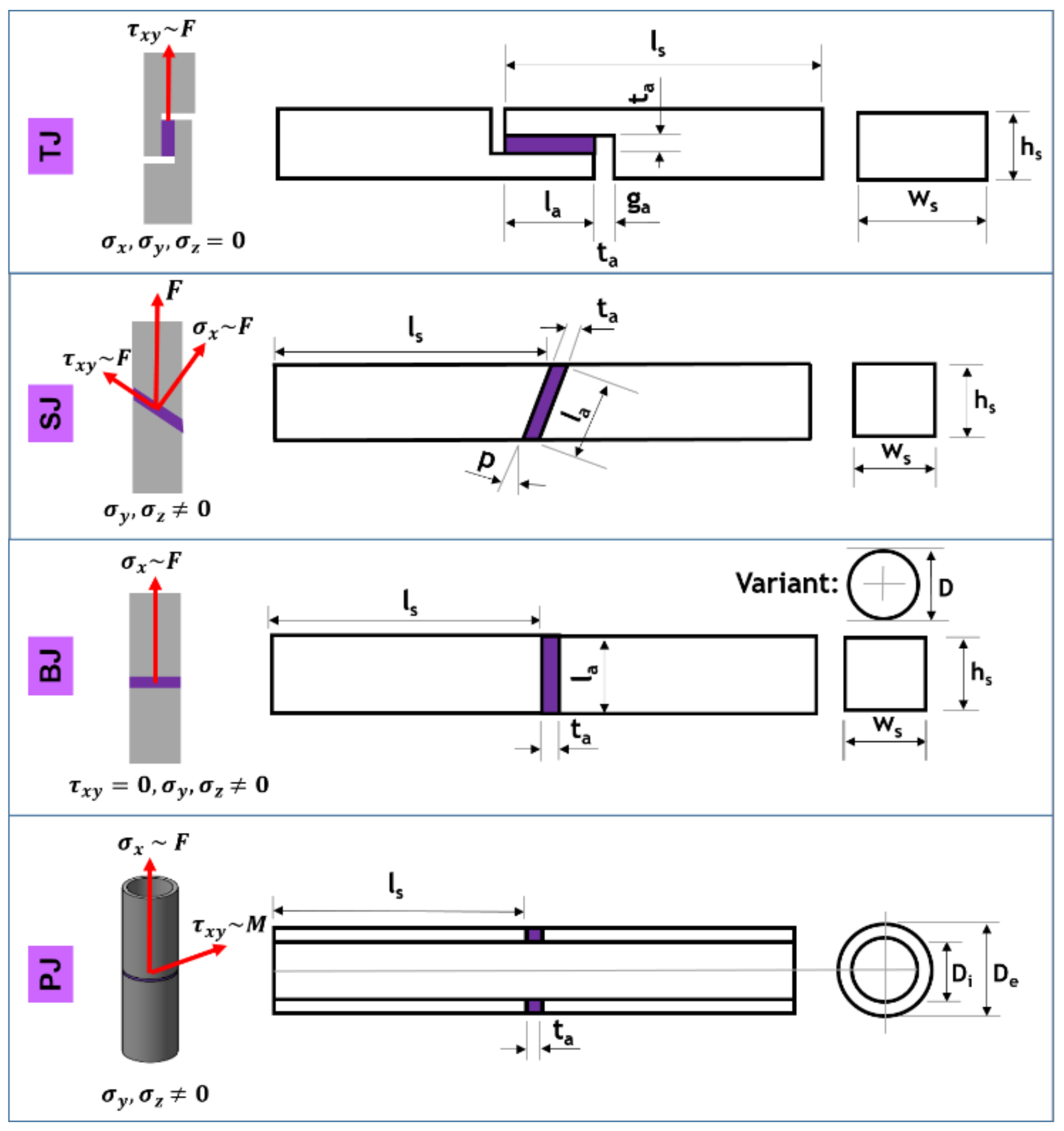
2.3. Adhesives and Joints

Adhesives have a particularity of usually being employed in a joint, i.e., to join two different substrates. Therefore, to properly investigate the lifetime prediction of structural adhesively bonded joints, it is important to not only have a variety of adhesives, but also a variety of joint types [46]. The data were modeled so as to describe the loading of the adhesive joint by comprising it of shear stress ( τ ) and tensile stress ( σ ) components:
  • Thick-Adherend-Shear-Test-Joint (TJ) → σ T J = 0 ,   τ T J 0
  • Scarf-Joint (SJ) → σ S J 0 ,   τ S J 0
  • Butt-Joint (BJ) → σ B J 0 ,   τ B J = 0
  • Pipe-Joint (PJ):
    -
    Pure Axial Load → σ P J , A x , 0 ,   τ T J , A x = 0 ;
    -
    Pure Torsional Load →   σ P J ,   T o = 0 ,   τ P J , T o 0 ;
    -
    Multiaxial Load → σ P J , M 0 ,   τ P J , M 0 .
As shown in Figure 2, the TJ is loaded under axial load F , generating a shear stress on the adhesive layer. The axial loading   F of the SJ generates a multiaxial state of stress comprising shear and tensile components. For the BJ, when loaded axially with F , a pure tensile stress state is obtained. Finally, the PJ has a larger variation, as it can be either loaded with axial load F (pure tensile stress), torsional load M (pure shear stress), or with both (multiaxial stress state). An additional influence for the PJ can be a phase-shift ϕ between the axial and torsional loads, which leads to a non-proportional loading.
Considering that the tensile stress is given in the x-direction (normal to the adhesive layer), as shown in Section 3.3, the restraint of the lateral contraction due the stiff substrates leads to the formation of two extra tensile stresses ( σ y and σ z ).
The geometric parameters (such as adhesive layer thickness t a ) were not taken into consideration for the prediction models described in Section 3. This could present a limitation of the prediction models. However, as these geometric parameters were, in some cases, only listed as target values (and not the actual values), it was not possible to include them on the modeling.
In Table 3, the distribution/quantity of each joint according to adhesives is given.

3. Prediction Models

To address the objective of the current investigation, which is to determine the best approach for the fatigue lifetime prediction of structural adhesive joints, four types of prediction models were implemented:
  • Data-driven models (DDMs);
  • A physics-based model (PBM);
  • Hybrid models (HM):
    -
    Hybrid models based on Findley’s critical plane (HM-F);
    -
    Hybrid models based on invariant stresses (HM-I).
The prediction models will be compared in terms of complexity of implementation, accuracy, and sensitivity to dataset size. The fatigue dataset will be split into train set and test set. An optimal balance should be found between train and test sets [47]. If the train set is too large, the generalization of the model cannot be tested, as the test dataset would be too limited. On the other hand, if the test set is too large, fewer samples would be available for the train set, which affects the overall performance of the model, as more train data tends to yield better models [48].
The accuracy will be quantified based on the two indicators: the coefficient of determination (R2) and the error factor (ER) for both the train and test datasets [32]:
E R = 1 n i = 1 n 10 l o g N p r e d , i l o g N e x p , i  
ER indicates the average error between the predicted lifetime ( N p r e d ) obtained from the prediction models and expected lifetime ( N e x p ) . As a reference value, in case of expected lifetime (correct value) of 1000 cycles, if the predicted lifetime is either 500 or 2000 cycles, both would lead to an ER of 2. For a perfect agreement ( N p r e d = N e x p ), an ER = 1 would be obtained.
To assess the sensitivity of each model to dataset size, three different splits of the fatigue dataset were investigated:
  • Split 70tr/30te: 70% of dataset for training and 30% for testing;
  • Split 50tr/50te: 50% of dataset for training and 50% for testing;
  • Split 30tr/70te: 30% of dataset for training and 70% for testing.
The proportions of each split were kept among each adhesive to ensure an equally distributed (balanced) dataset. A random shuffle of the dataset for each adhesive was carried out. Then, the split was done per each adhesive, which was followed by the combination into a single dataset (train and test set). The different splits, and respective sizes of the train (tr) and test (te) datasets are listed in Table 4.
Some procedures regarding the data treatment and feature selection were common to all models, including:
  • The fatigue lifetime (number of cycles to failure, N) was modeled using a logarithm scaling based on domain knowledge (e.g., the Basquin’s law [49]);
  • By assuming an ideal cohesive failure, and by the fact that the substrates were thick (little deformation), the predictions were carried out ignoring the substrate properties;
  • The geometric parameters of the joints were not taken into consideration;
  • The frequency ( f ) was not taken into consideration.

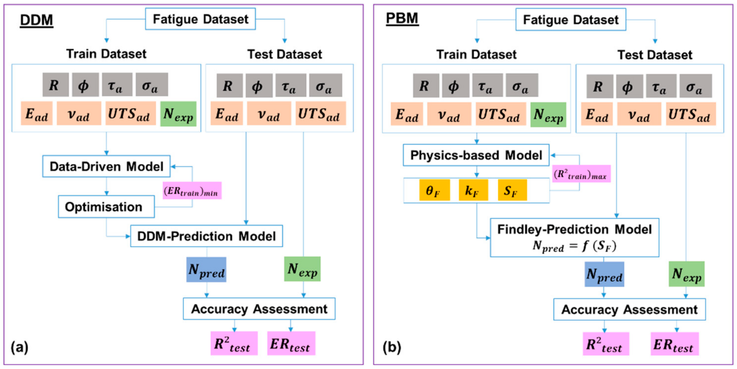
3.1. Data-Driven Model (DDM)

The workflow for the implementation of the DDM is presented in Figure 3a. The DDM was implemented as follows:
  • A particular data split (70Tr/30Te, 50Tr/50Te, or 30Tr/70Te) was selected;
  • Parameters of the train dataset (R, ϕ , τ a , σ a , E a d , U T S a d , N e x p ) were used to train the model;
  • The hyperparameters for the DDM are optimized so as to minimize ER_train (convergence criterion);
  • The trained DDM was determined;
  • Parameters of the test dataset (R, ϕ , τ a , σ a , E a d , U T S a d ) were used to test the DDM. However, the expected number of cycles to failure ( N e x p ) was not used as an input;
  • The output of the DDM was the predicted number of cycles to failure ( N c a l c );
  • The accuracy indicators of the DDM (R2_test and ER_test) were calculated based on N c a l c and N e x p .
Figure 3. Workflow of the (a) data-driven model (DDM) and (b) physics-based model (PBM).
Applmech 04 00019 g003
The model optimization was carried out by a five-fold cross-validation (see Appendix A) with grid search, i.e., four folds were employed as the train dataset and one fold as a validation dataset. With a grid search, all potential combinations in the hyperparameter sub-space are generated. After optimization of the model, the hyperparameter combination, which outperforms the others, was selected. The five-fold cross-validation also contributes to avoiding issues with overfitting [30]. The hyperparameter space for the optimization for the DDM (and HMs) is given in Table 5.
Since several regressors are available for data-driven prediction models, another relevant aspect of the current investigation was to determine which regressor would be the most suitable for the lifetime prediction considering the existing dataset (and their respective parameters). Four different regressors were evaluated for the development of the DDM, with each of them following the same procedure described in the workflow. All four regressors rely on the construction of non-linear relationships to achieve the best prediction. The regressors were:
  • Extra trees regressor (ERT, Python-library: sklearn) [50]: the ERT builds multiple decision trees on random subsets of the data and features. For each split in the tree, a random subset of features is chosen, and the best split is selected based on some criterion, such as reducing the variance or the mean squared error. The final prediction is made by averaging the predictions of all the trees.
  • ExtremeXGBoost regressor (XGB, Python-library: xgboost) [51]: the XGB uses gradient boosting to build a sequence of trees, where each tree tries to correct the errors made by the previous tree. The gradient boosting process starts with a weak base learner, such as a decision tree, and trains the next tree to correct the residuals from the previous tree. The final prediction is made by summing up the predictions of all the trees.
  • LightGBM regressor (LGBM, Python-library: lightgbm) [52]: the LGBM uses gradient boosting to build a sequence of trees, where each tree tries to correct the errors made by the previous tree. The algorithm uses a novel approach to build trees, called the histogram-based method, which reduces the computational cost compared to traditional gradient boosting algorithms. The histogram-based method splits the data based on histograms of feature values instead of finding the best split by brute force. The final prediction is made by summing up the predictions of all the trees.
  • Histogram-based gradient boosting regressor (HGB, Python-library: sklearn) [53]: the HGB is similar to XGB in that it also uses gradient boosting to build a sequence of trees. Moreover, the HGB is inspired (with slight modifications) by the LGBM.
The regressors were compared in terms of accuracy and sensitivity to data size. As the datasets were relatively small (n < 1000), the comparison of computational performance was not necessary.

3.2. Physics-Based Model (PBM)

For the physics-based model (PBM), the aim was to find a fatigue failure criterion so as to correlate the value of the criterion with the number of cycles to failure [1]. Considering the type of parameters available for the lifetime prediction with: different values of stress ratio ( R ), multiaxial stresses ( τ a and σ a ), as well as non-proportional loading ( ϕ 0 ° ) , the usage of a critical-plane stress-based criterion is a suitable approach [54]. In the concept of critical-plane, the multiaxial stress state is reduced to an equivalent uniaxial state in a specific plane. The idea is then to combine the normal and shear stresses in this fixed (critical) plane [54]. With this method, it is possible to calculate the fatigue life as well the position of the fatigue fracture plane.
The Findley’s critical plane stress [55] value is defined as follows:
S F = max τ a , C P θ F + k F σ m a x , C P ]
Here, S F is the value of the Findley’s stress, θ F is the angle of the critical plane,   k F is a material parameter related to the sensitivity to normal stress, τ a , C P is the shear stress amplitude at the critical plane, and σ m a x , C P is the upper normal stress at the critical plane.
Considering the train dataset, the process of determination of the critical plane and the Findley’s stress involved three loops through: (i) the normal stress sensitivity ( k F ), which varied from 0.0 to 2.0; (ii) one stress cycle (with shear and tensile stresses), which was divided into 100 time increments; and (iii) the angle θ F   of the plane, which varied from 0° to 180°. For a given number of cycles to failure ( N ), the calculations started by defining a given k F (e.g., k F = 0.1). Then, for each time increment, the plane was rotated from 0° to 180° with steps of 3° (see Figure 1b). The Findley’s stress { S F = max τ a , C P θ F + k F σ m a x , C P ] } was calculated for each plane. The maximum value S F was then recorded for every time increment. At the end, the plane with the largest value of S F was assumed as the critical plane. Therefore, for the given data point, a relationship was established between S F and N .
Finally, by taking the entire train dataset, the value of k F was determined so as to maximize R2_train for a regression of log N = f log S F , see Figure 1c. For the test dataset, the Findley’s stress ( S F ) was used as input to obtain the number of cycles to failure based on the previous relationship ( log N = f log S F ).
The workflow for the implementation of the PBM is presented in Figure 3b. The PBM was implemented as follows:
  • A particular data split (70Tr/30Te, 50Tr/50Te, or 30Tr/70Te) was selected;
  • Since the value of k F is adhesive-dependent, each adhesive was evaluated separately;
  • Parameters of the train set (R, ϕ , τ a , σ a , E a d , U T S a d , N e x p ) were used to train the model of each adhesive;
  • Train set: the value of k F was varied between 0 and 2.0;
  • Train set: for each data point the value of θ F was varied to maximize S F ;
  • Train set: the value of k F leading to the maximum correlation of R2_train between S F and N e x p (converge criterion) was determined;
  • The optimized PBM determined the relationship: log N p r e d = f log S F ;
  • Based on the parameters of the test dataset (R, ϕ , τ a , σ a , E a d , U T S a d ) the value of S F was used to test the PBM of each adhesive. However, the expected number of cycles to failure ( N e x p ) was not used as an input;
  • The output of the PBM was the predicted number of cycles to failure ( N c a l c );
  • The N c a l c and N e x p for each adhesive were combined;
  • The accuracy indicators of the PBM (R2_test and ER_test) were calculated based on N c a l c and N e x p .

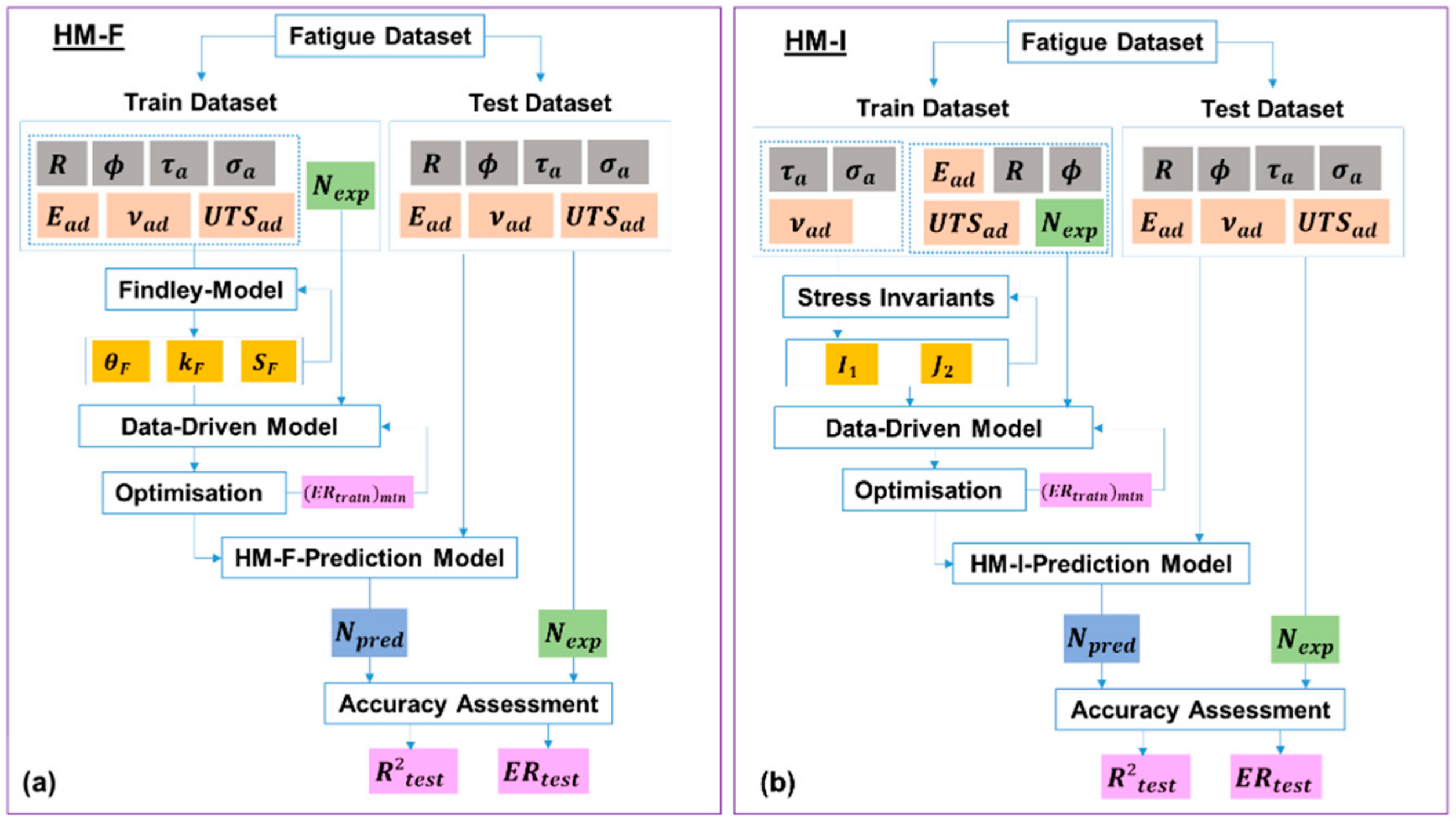
3.3. Hybrid Models (HM)

The hybrid models (HM) were developed to combine advantages of both of the DDM and the PPM. Two hybrid models were investigated:
  • A hybrid model using physics-based parameters from the Findley’s critical plane into a data-driven model (HM-F);
  • A hybrid model using physics-based stress invariant parameters into a data-driven model (HM-I).

3.3.1. Hybrid Model Using the Findley’s Critical Plane Approach (HM-F)

The HM-F relies on the usage of Findley’s approach to calculate k F ,   θ F , and S F . To use them, subsequently, as inputs for a DDM. The workflow of the HM-F is presented in Figure 4a:
  • A particular data split (70Tr/30Te, 50Tr/50Te, or 30Tr/70Te) was selected;
  • Since the value of k F is adhesive-dependent, each adhesive was evaluated separately;
  • Parameters of the train dataset (R, ϕ , τ a , σ a , E a d , U T S a d , N e x p ) were used to train a PBM of each adhesive;
  • Train set: the value of k F leading to the maximum correlation R2_train between S F and N e x p was determined;
  • The physics-based parameters of the train dataset ( k F , S F , θ F , E a d , U T S a d , N e x p ) were used to train a DDM regressor;
  • The hyperparameters of the DDM regressor were optimized so as to minimize the ER_train (convergence criterion);
  • The trained HM-F was determined;
  • Parameters of the test dataset (R, ϕ , τ a , σ a , E a d , U T S a d ) were used to test the HM-F. However, the expected number of cycles to failure ( N e x p ) was not used as an input;
  • The output of the HM-F was the predicted number of cycles to failure ( N c a l c );
  • The N c a l c and N e x p for each adhesive were combined;
  • The accuracy indicators of the HM-F (R2_test and ER_test) were calculated based on N c a l c and N e x p .
Figure 4. Workflow of the hybrid model: (a) based on Findley’s critical plane (HM-F) and the hybrid model (b) based on the invariant stresses (HM-I).
Applmech 04 00019 g004

3.3.2. Hybrid Model Using Invariant Stresses (HM-I)

The HM-I relies on the usage of invariant stresses to employ them afterwards as inputs for a DDM. Stress invariants have been widely employed in fatigue predictions approaches [31,32,33,56] as they provide relevant information on the stress state within the adhesive layer, such as the deviatoric stress (related to the shape change) and the hydrostatic stress (related to the volume change).
The stress invariants were defined as follows: taking x as the direction normal to the adhesive layer, and y and z as the transverse directions, a generic 3D stress tensor can be constructed for the adhesive layer in order to describe its stress state:
σ = σ x τ x y 0 τ x y σ y 0 0 0 σ z
With the assumption of homogenous stress distribution and a complete transverse strain restraint of the adhesive layer due to the higher stiffness of the substrates (substrate ca. 10 times stiffer than the adhesive). It can be inferred from the linear elasticity that:
σ y = σ z = v a d 1 v a d σ x  
where   v a d is the Poisson’s ratio of the adhesive.
The stress invariants, i.e., stress values that are independent of the coordinate system, I 1 and J 2 can be defined as follows:
I 1 = σ x + σ y + σ z  
J 2 =   1 3 [ σ x 2 + σ y 2 + σ z 2 σ x σ y σ x σ z σ y σ z ] + τ x y 2
The stress invariants ( I 1 , J 2 ) are relevant parameters for the determination of the behavior of adhesive joints. They can be correlated with the hydrostatic stress ( σ H ) and deviatoric stress (i.e., von Mises stress, σ V M ), which are strongly related to the fatigue behavior of adhesives as shown in [31,57,58].
σ H = I 1 3
σ V M = 3 J 2
The workflow of the HM-I is presented in Figure 4b:
  • A particular data split (70Tr/30Te, 50Tr/50Te, or 30Tr/70Te) was selected;
  • Train dataset: based on parameters ( τ a , σ a ,   ν a d ) the invariant stresses ( I 1 and J 2 ) were calculated;
  • The physics-based parameters of the test dataset ( I 1 , J 2 , ϕ , E a d , U T S a d ,   N e x p ) were used to train a DDM regressor;
  • The hyperparameters of the DDM regressor were optimized so as to minimize the ER_train;
  • The trained HM-I was determined;
  • Parameters of the test dataset (R, ϕ , τ a , σ a , E a d , U T S a d ) were used to test the HM-I. However, the expected number of cycles to failure ( N e x p ) was not used as an input;
  • The output of the HM-I was the predicted number of cycles to failure ( N c a l c );
  • The N c a l c and N e x p for each adhesive were combined;
  • The accuracy indicators of the HM-I (R2_test and ER_test) were calculated based on N c a l c and N e x p .

4. Prediction Results

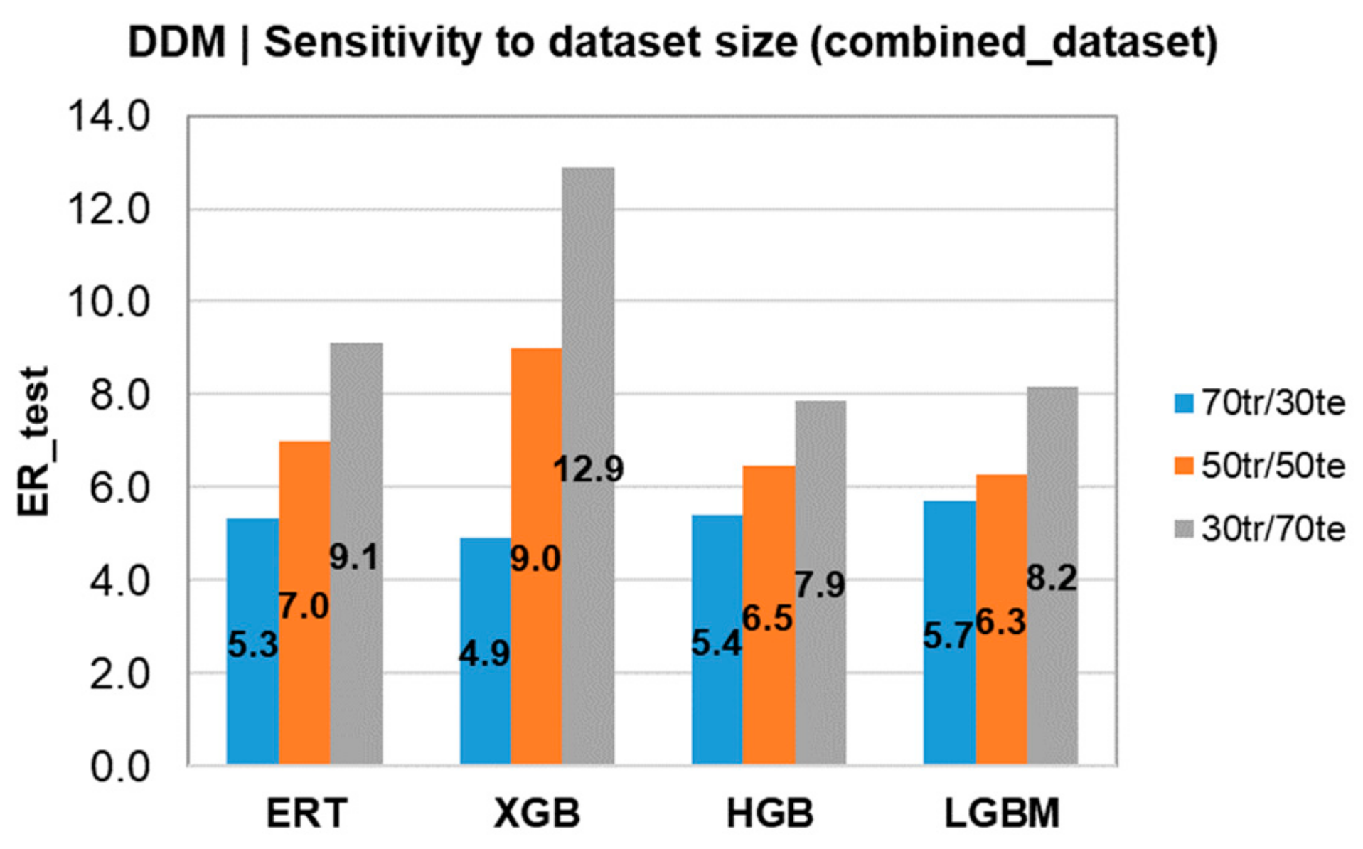
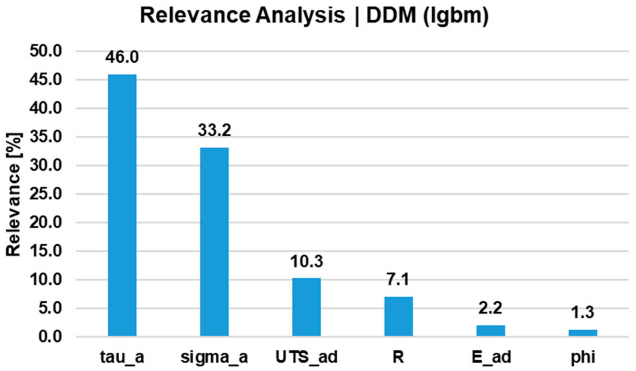
4.1. Predictions by Data-Driven Models

The predictions related to the data-driven models (DDMs) were carried out following the workflow shown in Figure 3a. For that approach, four ML methodologies were applied: extra trees regressor (ERT), XGBoost regressor (XGB), histogram-based gradient boosting (HGB), and LightGBM (LGBM).
The first assessment performed is related to the accuracy of each methodology to predict the test data according to the size of the train dataset. In Table 6, one can find a summary of the results obtained in the prediction of the train and test data regarding the (R2_train/R2_test) and (ER_train and ER_test) scores. On the one hand, ERT and XGB predictions presented very high R2_train (low ER_train) values for the train dataset, but were not able to repeat their good performance using the test data (R2_test or ER_test), which is an indication of less generalization power. On the other hand, HGB and LGBM prediction performances showed less variation when comparing R2_train values to R2_test values.
The ER_test values for predictions with the DDM according to split size and the regressor method are given in Figure 5. Based on the evaluation of each ML-methodology applied, the following assessments can be drawn: (i) the accuracy in predicting the test data was strongly influenced by the train dataset size. The best prediction accuracy was achieved when the size of the train dataset increased (70tr/30te); (ii) HGB and LGBM predictions showed less sensitivity to the size of the train dataset compared to the other methods; (iii) in terms of ER when comparing the results of the 70tr/30te and 30tr/70te split datasets, the accuracy of the models changed. The LGBM lost 1.46x its performance (ER from 5.7 to 8.2), and the XGB had the largest reduction of performance with 2.63x (ER from 4.9 to 12.9); and, (iv) the XGB showed the highest accuracy for the 70tr/30te split with ER = 4.9.
In Figure 6, the relevance analysis of each parameter for the DDM (lgbm) is given. This technique assigns a score to each parameter to determine how useful each input is in predicting a desired variable, in this case, the number of cycles to failure (N). Important information can be obtained from the relevance output of this technique: (i) “tau_a” and “sigma_a” show the higher values of relevance for the model predictions; (ii) “UTS_ad” plays a greater role for the DDM predictions than “R” and “E_ad”; and (iii) most of the data used for training and testing of DDMs have “phi” values of 0°; hence, the relevance of this input is smaller.

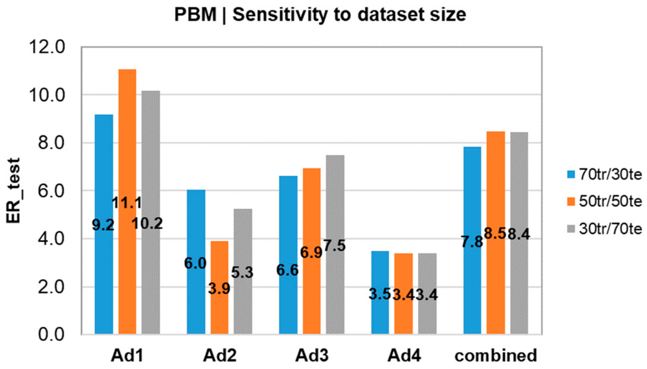
4.2. Predictions Using the Physics-Based Model

In terms of the physics-based model (PBM), predictions were carried out following the workflow shown in Figure 3b. For that approach, the Findley’s failure criterion (Equation (7)) is applied. The first findings are related to the sensitivity of the PBM to dataset size. In Table 7, the R2_train/R2_test indicators are given as a function of the data split. Contrarily to the DDM, in the PBM, the R2_train and R2_test values were more comparable. However, the value of k F varied according to the size of dataset. Nonetheless, with enough train data, the value of k F tends to be very close for every adhesive.
In Figure 7, the values of ER_test are given per each adhesive, as well as the combined dataset. The change in the size of the trained/tested dataset seems to be less relevant for the accuracy of the model predictions, i.e., increasing the dataset size will not likely be beneficial for future predictions. This could be observed, for instance, in the prediction of the Ad1, which, despite having the largest dataset, presents the highest ER_test. Considering the split 70tr/30te, the prediction of the combined_testset was more accurate in the DDM-xgb (ER_test = 4.9) as compared to the PBM (ER_test = 7.8).

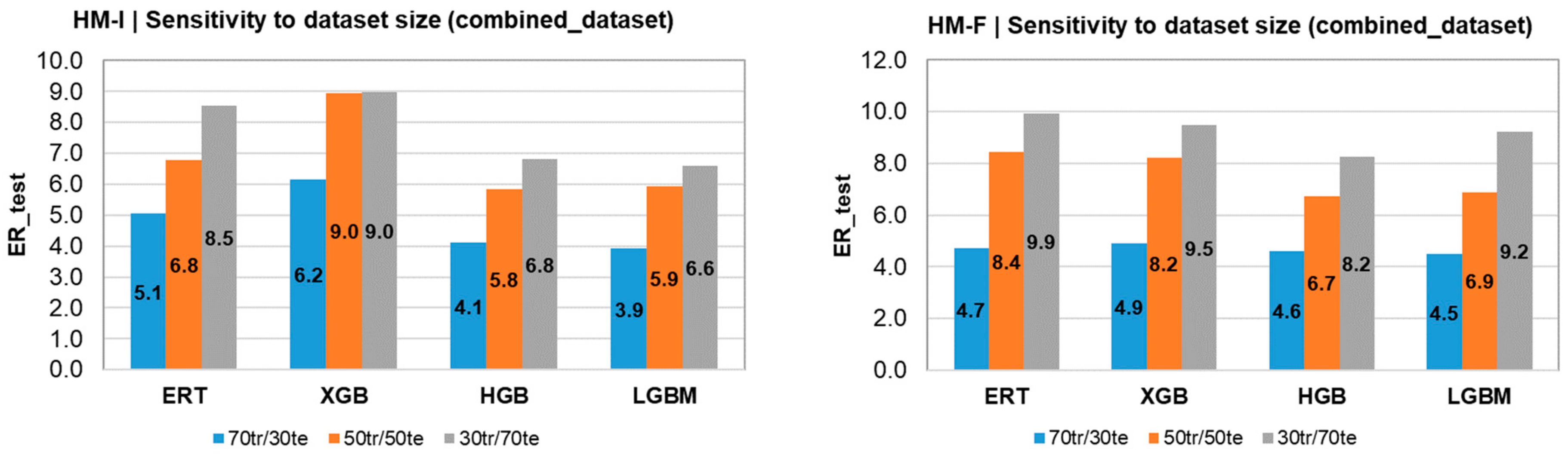
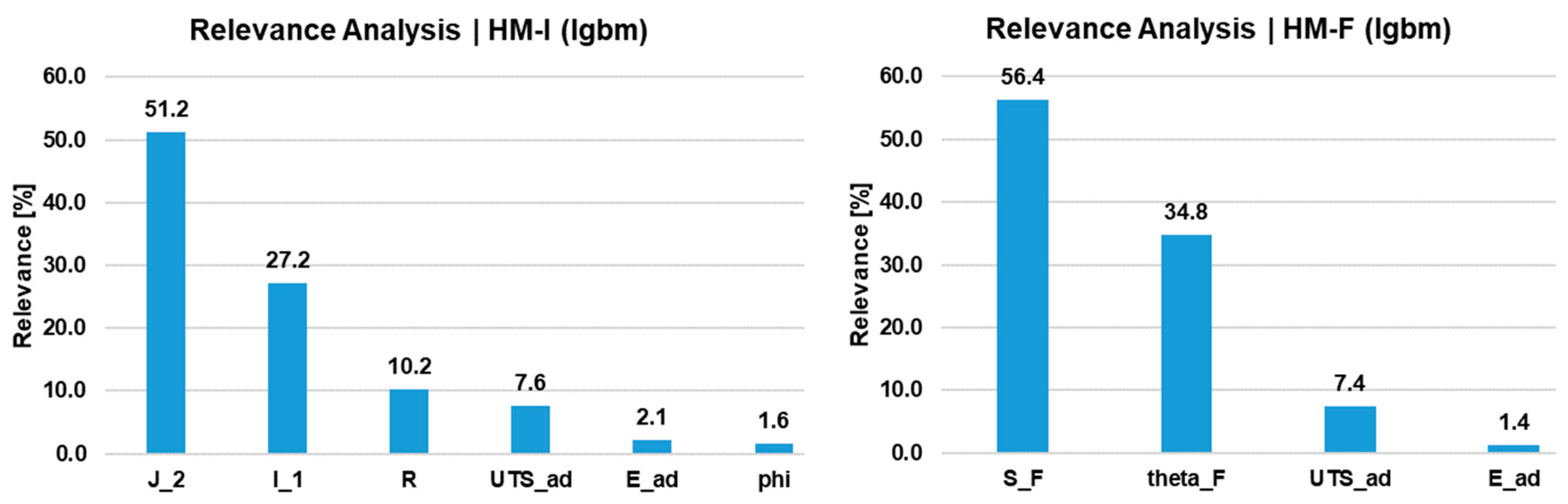
4.3. Predictions Using Hybrid Models

As defined in Section 3.3, the proposal for hybrid models is to use the same ML-methods applied in the DDM, but with the introduction of stress-based parameters obtained from physics-based approaches as input parameters. The models have been divided according to the applied inputs. While the HM-I introduces the stress invariants ( I 1 , J 2 ) as inputs parameters, the HM-F introduces the angle ( θ F ) and Findley’s stress criterion ( S F ) obtained from the PBM. In the workflow presented in Figure 4a,b, one can find how predictions were carried out. As performed for DDM and PBM, the first assessment is related to the accuracy of the model to predict the test data based on the train dataset size (sensitivity to dataset size).
In Table 8 and Table 9, the R2_train and R2_test according to dataset split and regressor are given. Similarly to the DDM, for both the HM-I and HM-F, ERT and XGB regressors yielded high R2_train (low ER_train) values, but were not able to repeat their good performance using the test data, i.e., R2_test values (less generalization power). On the other hand, HGB and LGBM prediction performances presented less variation when comparing R2_train (ER_train) values to R2_test (ER_test) values.
In Figure 8, the ER_test for the HM-I and HM-F models is given according to the data split and ML regressor method. Based on prediction results, it is possible to note the following: (i) on average HM-I shows higher accuracy for the test data, when compared to the HM-F (1.15x more accurate using LGBM for the 70tr/30te split); (ii) the accuracy in predicting the test data was strongly influenced by the trained dataset size for both approaches; and (iii) LGBM produces the best prediction results for both HM-I and HM-F.
The parameter relevance analysis for the hybrid models is provided in Figure 9. Considering the HM-I, J_2 and I_1 were the most relevant parameters (even more relevant than “tau_a” and “sigma_a” for the DDM). Moreover, “R” plays a greater role for the HM-I predictions than “UTS_ad” and “E_ad”. For the HM-F, “S_F” and “theta_F” have the highest relevance for predictions. Since most of the data used for the training and testing of the hybrid models have “phi” values of 0°, the relevance of this input is minimal for both HM-I and HM-F.

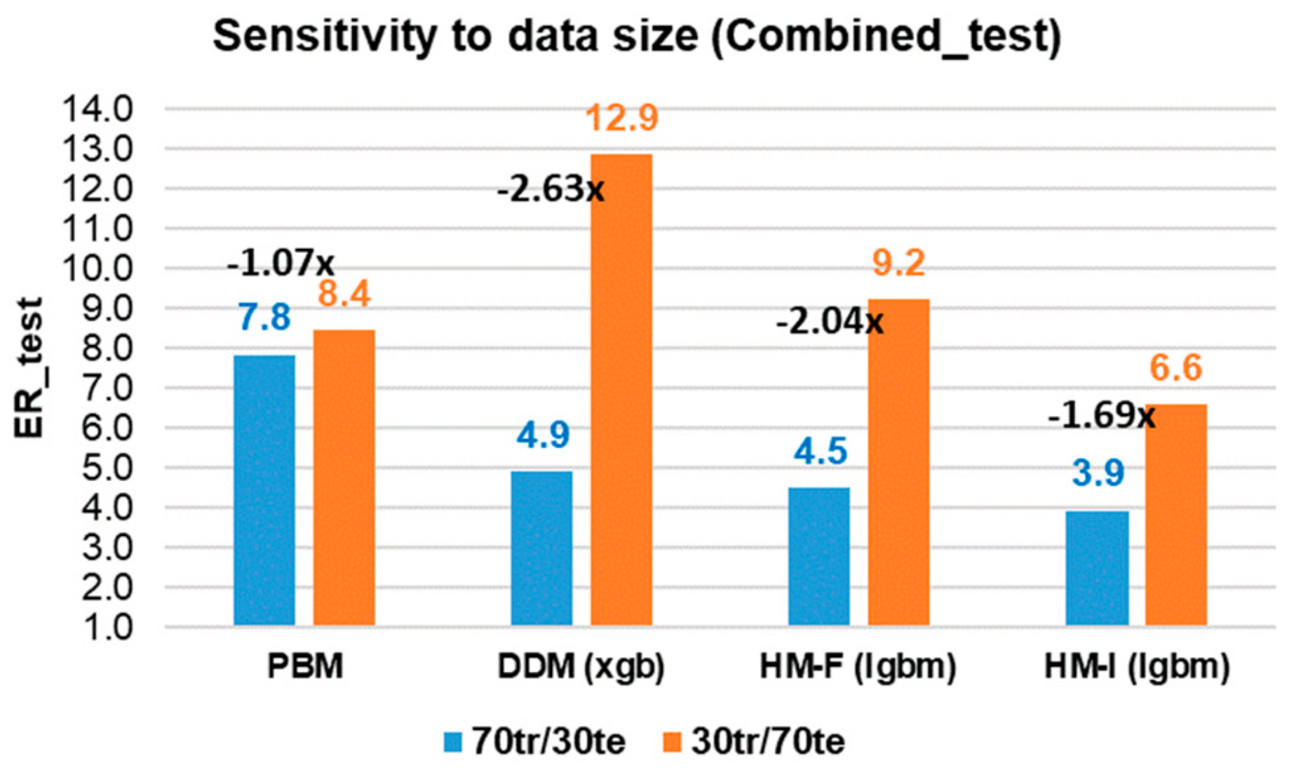
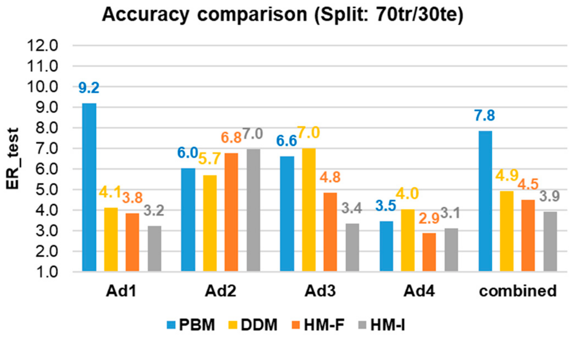
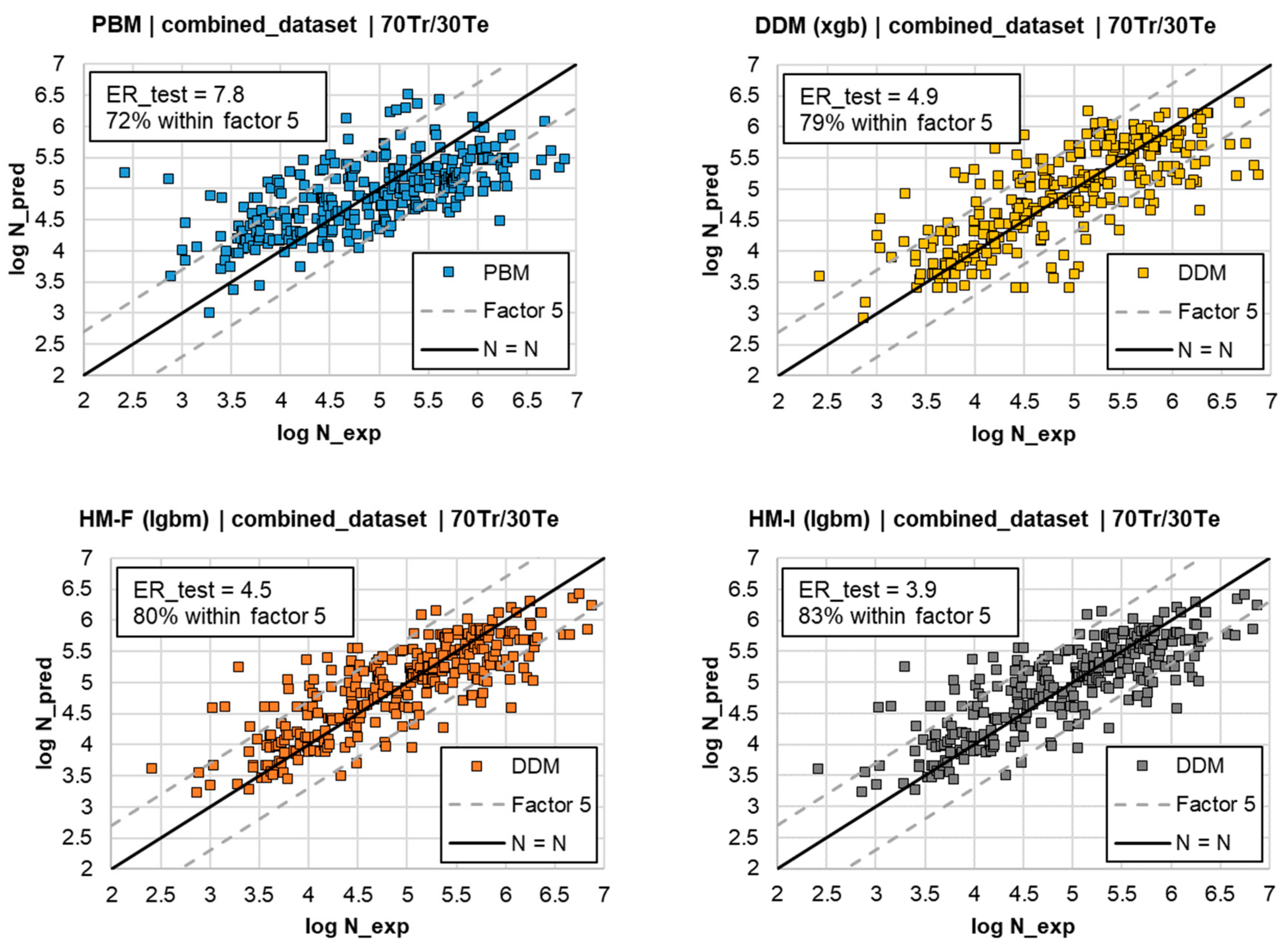
4.4. Performance Comparison between Models and Outlook

As a summarizing step, the performance of the four models (DDM, PBM, HM-I, and HM-F) was compared in terms of sensitivity to data size, accuracy, and complexity of implementation. In Figure 10, the ER_test for the prediction models as a function of the data split (70tr/30te and 30tr/70te) is shown. The PBM has the smallest reduction of accuracy with −1.07x. Hybrid models (HM-F and HM-I) are less sensitive to the data size than the DDM. The accuracy of the DDM decreased 2.63 times, compared to −2.04x of the HM-F and −1.69x to the HM-I. Therefore, one could infer that the HMs combine the accuracy improvement of the DDM, with the robustness to data size of the PBM.
Figure 11 presents the accuracy of models (ER_test) for each adhesive and for the combined dataset taking the 70tr/30te split. The hybrid models have the highest accuracy, especially the HM-I with an accuracy for the combined dataset within a factor of four lifetimes (ER_test = 3.9). This accuracy improvement is reflected in three out four adhesives (except Ad2). The HM-I was able to improve the accuracy of the DDM in 20% whereas, for the HM-F, this improvement was of 8%. Comparatively, the PBM has the lowest accuracy for the combined dataset.
Considering the 70tr/30te split, 296 data points were predicted in the test dataset. The N_pred/N_exp plot for the prediction using the four models (DDM, PBM, HM-I, and HM-F) is given in Figure 12. The black diagonal lines establish a perfect prediction, whereas the gray dashed lines define a region within a factor of five lifetimes. As an additional accuracy metric, not only the ER_test is provided, but also the percentage of the data points, which are within a factor of five lifetimes (ER_test < 5). For the HM-I, 83% of predictions are within a factor of five, followed by the HM-F with 80%, the DDM with 79%, and the PBM with 72%.
Another investigation regarding the hybrid models was carried out in order to assess whether the accuracy of the combined dataset is higher than that of a single adhesive, i.e., (i) train the model with adhesive A, and test with adhesive A or (ii) train the model with a combined adhesive dataset (including A), and test with a combined adhesive dataset (including A). The discussion here would be: “is it more relevant to have a homogeneous dataset (A predicting A) or to have more data available (combined predicting combined)?”. Table 10 shows the prediction accuracy (ER_test) using the HM-I for a 70Tr/30Te split considering two different datasets: (i) homogeneous prediction (A predicting A) and (ii) heterogeneous prediction (combined predicting combined).
For all adhesives, the predictions with the heterogeneous dataset outperformed the homogeneous dataset. Moreover, for the adhesive with the smallest dataset (Ad4), there was not enough data to reach a minimum convergence criterion. Nonetheless, for the same adhesive, with the use of the heterogeneous dataset (with the combination of information from other adhesives), it was possible to obtain a very good accuracy for the Ad4.
Another relevant aspect is that complexity of the implementation for the four models was comparable. The most demanding task was related to the preparation of the dataset, including data mining, data cleaning, data curation, and feature selection. In terms of computational time, all models were within the same range. The models were executed using the Jupyter © Notebook in a PC (Intel© i5-10400H (2.6 GHz) with 16GB of RAM). For this reason, the implementation of the hybrid models can be a method for improvement of lifetime prediction (accuracy and minimum required data). Hybrid modelling also allows a reduction in the number of experiments by taking advantage of the accuracy of data-driven models, and robustness of data size of physics-based models. Finally, the use of hybrid models, which rely on physics-based approaches, might enhance the acceptance of AI-based solutions in engineering fields, as more explainable (or more visible) correlations between parameters and predictions can be assessed.

5. Conclusions

In the current work, a comparative investigation of data-driven, physics-based, and hybrid models for the fatigue lifetime prediction of structural adhesive joints was presented. Four data-driven models (DDM) were constructed using extremely randomized trees (ERT), eXtreme gradient boosting (XGB), LightGBM (LGBM), and histogram-based gradient boosting (HGB). The physics-based model (PBM) relies on the critical plane approach. Two hybrid models were developed by combining data-driven approaches with physics-based parameters obtained from the invariant stresses (HM-I) and the Findley’s critical plane approach (HM-F).
A fatigue dataset was constructed with 979 fatigue data points from four structural adhesives with four joint configurations. To assess the sensitivity to data size, the fatigue dataset was split with three different ratios of train/test dataset, namely 70%/30%, 50%/50%, and 30%/70%. Prediction accuracy is evaluated from the R2 and the error factor (ER) for the test datasets from lifetime predictions.
Results revealed that DDMs are more accurate, but more sensitive to the dataset size when compared to the PBM. At the same time, DDMs have the potential of accuracy improvement with the extension of the database. Among different regressors, the LGBM presented the best performance when dealing with smaller and larger train datasets. HMs increased the accuracy of predictions, whilst enhancing the robustness of models (reduction of sensitivity to data size). Finally, the HM-I showed the highest accuracy with an improved sensitivity to data size compared to the DDMs. Considering the HM-I, for all adhesives, predictions with the heterogeneous dataset outperformed the homogeneous dataset.

Author Contributions

Conceptualization, P.H.E.F. and V.C.B.; code development, P.H.E.F. and G.C.S.; validation and formal analysis, P.H.E.F. and V.C.B.; data curation, M.S.; discussion, P.H.E.F., G.C.S., D.B.P. and V.C.B.; writing—review and editing, P.H.E.F. and V.C.B.; supervision, C.N. and K.K. All authors have read and agreed to the published version of the manuscript.

Funding

This research has received funding in the framework of the DOME4.0 project from the European Union’s Horizon 2020 Research and Innovation Programme under Grant Agreement No. 953163. V. C. Beber acknowledges the funding from CAPES (Coordenaçao de Aperfeiçoamento de Pessoal de Nível Superior) through the Science without Borders program (grant BEX 13458/13-2).

Data Availability Statement

Research data are not shared.

Acknowledgments

The authors would like to thank the Editorial Board of Applied Mechanics for the waiving of the APC.

Conflicts of Interest

The authors declare no conflict of interest.

Abbreviations

The following abbreviations/symbols were employed in this investigation:
Abbreviation/SymbolMeaning
AIArtificial intelligence
adAdhesive
BJButt Joint
DDMData-driven model
EYoung’s modulus in [MPa]
ERError factor
ERTExtremely randomized trees
HGBMHistogram-based gradient boosting model
HM-FHybrid model based on Findley’s critical plane model
HM-IHybrid model based on invariant stress
LGBMLight gradient-boosting method
LLNLaw of large numbers
MLMachine learning
NNumber of cycles to failure
nNumber of observations
PBMPhysics-based model
PJPipe Joint
RStress ratio
RFRandom forest
SJScarf Joint
subSubstrate
teTest
trTrain
TJThick-Adherend-Shear-Test Joint
UTSUltimate tensile strength in [MPa]
XGBGradient boosting method
ϕ Phase-shift in [°]
τ Shear stress in [MPa]
σ Tensile stress in [MPa]
θ F   ( or   theta _ F ) Angle of Findley’s critical plane
ν Poisson’s ratio
S F   ( or   S _ F ) Findley’s critical stress
k F   ( or   k _ F ) Findley’s normal stress sensitivity
I 1   ( or   I _ 1 ) First invariant of the principal stress tensor in [MPa]
J 2   ( or   J _ 2 ) Second invariant of the deviatoric stress tensor in [MPa]

Appendix A

Python Libraries employed for this investigation:
  • Data manipulation
    • import os
    • import pandas as pd
    • import xlwings as wx
    • import numpy as np
    • import math-Shuffle
    • from sklearn.utils import shuffle
  • Models applied
    • from sklearn.ensemble import ExtraTreesRegressor,HistGradientBoostingRegressor
    • import xgboost as xgb
    • import lightgbm as ltb
    • from sklearn.linear_model import LinearRegression
  • Model optimization
    • from sklearn.model_selection import GridSearchCV,cross_val_score,KFold,RepeatedKFold,RandomizedSearchCV
  • Cross-validation
  • cv = KFold(5, shuffle = True, random_state = None)
  • gsc = GridSearchCV(
  • estimator = ltbreg,
  • param_grid = {‘max_depth’: range(5,20,1),
  • ‘n_estimators’: (500)
  • ‘max_features’: [1,2,3,4],
  • ‘min_samples_split’: range(2,5,1)},
  • scoring = make_scorer(ER_loss,greater_is_better = False),
  • cv = cv,
  • verbose = 2, n_jobs = −1)
  • Figure manipulation
  • import matplotlib.pyplot as plt

References

  1. Da Silva, L.F.M.; Öchsner, A.; Adams, R.D. Handbook of Adhesion Technology; Springer: Berlin, Germany, 2011; ISBN 978-3-642-01168-9. [Google Scholar]
  2. Fraunhofer-Institut für Fertigungstechnik und Angewandte Materialforschung IFAM. In Circular Economy and Adhesive Bonding Technology; Fraunhofer Verlag: Stuttgart, Germany, 2020.
  3. Da Silva, L.F.M.; Öchsner, A. Modeling of Adhesively Bonded Joints; Springer: Berlin, Germany, 2008; ISBN 978-3-540-79055-6. [Google Scholar]
  4. Abdel Wahab, M.M. Fatigue in Adhesively Bonded Joints: A Review. ISRN Mater. Sci. 2012, 2012, 746308. [Google Scholar] [CrossRef]
  5. Matzenmiller, A.; Kumatowski, B.; Hanselka, H.; Bruder, T.; Schmidt, H.; Mayer, B.; Schneider, B.; Kehlenbeck, H.; Nagel, C.; Brede, M. Schwingfestigkeitsauslegung von Geklebten Stahlbauteilen des Fahrzeugbaus unter Belastung mit Variablen Amplituden: Forschung für Die Praxis P796, IGF-Nr. 307 ZN; Forschungsvereinigung Stahlanwendung e. V: Düsseldorf, Germany, 2012. [Google Scholar]
  6. Meschut, G.; Teutenberg, D.; Cavdar, S.; Melz, T.; Rybar, G.; Mayer, B.; Fiedler, A.; Nagel, C.; Matzenmiller, A.; Kroll, U. Analyse der Schwingfestigkeit Geklebter Stahlverbindungen unter Mehrkanaliger Belastung: Forschung für Die Praxis P1028, IGF-Nr. 18107 N; Forschungsvereinigung Stahlanwendung e. V: Düsseldorf, Germany, 2017. [Google Scholar]
  7. Beber, V.C.; Baumert, M.; Klapp, O.; Nagel, C. Multiaxial elastic, yield and failure behaviour of bonded joints using a hot-curing epoxy film adhesive: Analytical and experimental investigation. J. Adhes. 2020, 98, 526–552. [Google Scholar] [CrossRef]
  8. Beber, V.C.; Schneider, B. Fatigue of structural adhesives under stress concentrations: Notch effect on fatigue strength, crack initiation and damage evolution. Int. J. Fatigue 2020, 140, 105824. [Google Scholar] [CrossRef]
  9. Beber, V.C.; Schneider, B.; Brede, M. On the fatigue behavior of notched structural adhesives with considerations of mechanical properties and stress concentration effects. Procedia Eng. 2018, 213, 459–469. [Google Scholar] [CrossRef]
  10. Beber, V.C.; Fernandes, P.H.E.; Schneider, B.; Brede, M.; Mayer, B. Fatigue lifetime prediction of adhesively bonded joints: An investigation of the influence of material model and multiaxiality. Int. J. Adhes. Adhes. 2017, 78, 240–247. [Google Scholar] [CrossRef]
  11. Beber, V.C.; Schneider, B.; Brede, M. Influence of Temperature on the Fatigue Behaviour of a Toughened Epoxy Adhesive. J. Adhes. 2015, 92, 778–794. [Google Scholar] [CrossRef]
  12. Schneider, B.; Beber, V.C.; Brede, M. Estimation of the lifetime of bonded joints under cyclic loads at different temperatures. J. Adhes. 2015, 92, 795–817. [Google Scholar] [CrossRef]
  13. Schneider, B.; Beber, V.C.; Schweer, J.; Brede, M.; Mayer, B. An experimental investigation of the fatigue damage behaviour of adhesively bonded joints under the combined effect of variable amplitude stress and temperature variation. Int. J. Adhes. Adhes. 2018, 83, 41–49. [Google Scholar] [CrossRef]
  14. Baumgartner, J.; Schmidt, H.; Rybar, G.; Melz, T.; Ernstberger, L.J.; Teutenberg, D.; Hahn, O.; Meschut, G.; Nagel, C.; Schneider, B. Auslegung von Geklebten Stahlblechstrukturen im Automobilbau für Schwingende Last bei Wechselnden Temperaturen nter Berücksichtigung des Versaensverhaltens; No. 290; FAT: Frankfurt, Germany, 2016. [Google Scholar]
  15. Fernandes, P.H.E.; Poggenburg-Harrach, L.; Nagel, C.; Beber, V.C. Lifetime calculation of adhesively bonded joints under proportional and non-proportional multiaxial fatigue loading: A combined critical plane and critical distance approach. J. Adhes. 2022, 98, 780–809. [Google Scholar] [CrossRef]
  16. Bhadeshia, H.K.D.H. Neural Networks and Information in Materials Science. Stat. Anal. Data Min. 2009, 1, 296–305. [Google Scholar] [CrossRef]
  17. DOME4.0. Digital Open Marketplace Ecosystem 4.0. Available online: https://dome40.eu/ (accessed on 2 February 2023).
  18. NFDI-MatWerk. Nationale Forschungsdateninfrastruktur für Materialwissenschat & Werkstofftechnik. Available online: https://nfdi-matwerk.de/ (accessed on 2 February 2023).
  19. Zhao, S.; Qian, Q. Ontology based heterogeneous materials database integration and semantic query. AIP Adv. 2017, 7, 105325. [Google Scholar] [CrossRef] [Green Version]
  20. Zhang, Y.; Ling, C. A strategy to apply machine learning to small datasets in materials science. NPJ Comput. Mater. 2018, 4, 25. [Google Scholar] [CrossRef] [Green Version]
  21. Hao, W.Q.; Tan, L.; Yang, X.G.; Shi, D.Q.; Wang, M.L.; Miao, G.L.; Fan, Y.S. A physics-informed machine learning approach for notch fatigue evaluation of alloys used in aerospace. Int. J. Fatigue 2023, 170, 107536. [Google Scholar] [CrossRef]
  22. Karniadakis, G.E.; Kevrekidis, I.G.; Lu, L.; Perdikaris, P.; Wang, S.; Yang, L. Physics-informed machine learning. Nat. Rev. Phys. 2021, 3, 422–440. [Google Scholar] [CrossRef]
  23. Zhang, X.-C.; Gong, J.-G.; Xuan, F.-Z. A physics-informed neural network for creep-fatigue life prediction of components at elevated temperatures. Eng. Fract. Mech. 2021, 258, 108130. [Google Scholar] [CrossRef]
  24. Tang, A.; Tam, R.; Cadrin-Chênevert, A.; Guest, W.; Chong, J.; Barfett, J.; Chepelev, L.; Cairns, R.; Mitchell, J.R.; Cicero, M.D.; et al. Canadian Association of Radiologists White Paper on Artificial Intelligence in Radiology. Can. Assoc. Radiol. J. 2018, 69, 120–135. [Google Scholar] [CrossRef] [Green Version]
  25. Wei, J.; Chu, X.; Sun, X.-Y.; Xu, K.; Deng, H.-X.; Chen, J.; Wei, Z.; Lei, M. Machine learning in materials science. InfoMat 2019, 1, 338–358. [Google Scholar] [CrossRef] [Green Version]
  26. Zhu, Y.; Zhao, T.; Jiao, J.; Chen, Z. The lifetime prediction of epoxy resin adhesive based on small-sample data. Eng. Fail. Anal. 2019, 102, 111–122. [Google Scholar] [CrossRef]
  27. Mansouri, E.; Manfredi, M.; Hu, J.-W. Environmentally Friendly Concrete Compressive Strength Prediction Using Hybrid Machine Learning. Sustainability 2022, 14, 12990. [Google Scholar] [CrossRef]
  28. Zhou, K.; Sun, X.; Shi, S.; Song, K.; Chen, X. Machine learning-based genetic feature identification and fatigue life prediction. Fatigue Fract. Eng. Mater. Struct. 2021, 44, 2524–2537. [Google Scholar] [CrossRef]
  29. Heng, J.; Zheng, K.; Feng, X.; Veljkovic, M.; Zhou, Z. Machine Learning-Assisted probabilistic fatigue evaluation of Rib-to-Deck joints in orthotropic steel decks. Eng. Struct. 2022, 265, 114496. [Google Scholar] [CrossRef]
  30. Blakseth, S.S.; Rasheed, A.; Kvamsdal, T.; San, O. Combining Physics-Based and Data-Driven Techniques for Reliable Hybrid Analysis and Modeling Using the Corrective Source Term Approach. Appl. Soft Comput. 2022, 128, 1–20. [Google Scholar] [CrossRef]
  31. Çavdar, S.; Teutenberg, D.; Meschut, G.; Wulf, A.; Hesebeck, O.; Brede, M.; Mayer, B. Stress-based fatigue life prediction of adhesively bonded hybrid hyperelastic joints under multiaxial stress conditions. Int. J. Adhes. Adhes. 2020, 97, 102483. [Google Scholar] [CrossRef]
  32. Beber, V.C.; Schneider, B.; Brede, M. Efficient critical distance approach to predict the fatigue lifetime of structural adhesive joints. Eng. Fract. Mech. 2019, 214, 365–377. [Google Scholar] [CrossRef]
  33. Beber, V.C.; Baumert, M.; Klapp, O.; Nagel, C. Fatigue failure criteria for structural film adhesive bonded joints with considerations of multiaxiality, mean stress and temperature. Fatigue Fract. Eng. Mater. Struct. 2021, 44, 636–650. [Google Scholar] [CrossRef]
  34. Beugre, O.M.R.; Akhavan-Safar, A.; da Silva, L.F.M. Multiaxial Fatigue Life Assessment of Adhesive Joints Based on the Concepts of Critical Planes: Stress-Based Approaches. In Proceedings of the 6th International Conference on Adhesive Bonding 2021, Porto, Portugal, 8–9 July 2021; Da Silva, L.F.M., Adams, R.D., Eds.; Springer International Publishing: Cham, Switzerland, 2021; pp. 153–169, ISBN 978-3-030-87667-8. [Google Scholar]
  35. Chen, J.; Liu, Y. Fatigue modeling using neural networks: A comprehensive review. Fatigue Fract. Eng. Mater. Struct. 2022, 45, 945–979. [Google Scholar] [CrossRef]
  36. Leininger, D.S.; Reissner, F.-C.; Baumgartner, J. New approaches for a reliable fatigue life prediction of powder metallurgy components using machine learning. Fatigue Fract. Eng. Mater. Struct. 2022, 46, 1190–1210. [Google Scholar] [CrossRef]
  37. Sekercioglu, T.; Kovan, V. Prediction of static shear force and fatigue life of adhesive joints by artificial neural network. Met. Mater. 2008, 46, 51–57. [Google Scholar]
  38. Silva, G.C.; Beber, V.C.; Pitz, D.B. Machine learning and finite element analysis: An integrated approach for fatigue lifetime prediction of adhesively bonded joints. Fatigue Fract. Eng. Mater. Struct. 2021, 44, 3334–3348. [Google Scholar] [CrossRef]
  39. Schubert, M.; Kläusler, O. Applying machine learning to predict the tensile shear strength of bonded beech wood as a function of the composition of polyurethane prepolymers and various pretreatments. Wood Sci. Technol. 2020, 54, 19–29. [Google Scholar] [CrossRef]
  40. Pruksawan, S.; Lambard, G.; Samitsu, S.; Sodeyama, K.; Naito, M. Prediction and optimization of epoxy adhesive strength from a small dataset through active learning. Sci. Technol. Adv. Mater. 2019, 20, 1010–1021. [Google Scholar] [CrossRef] [PubMed] [Green Version]
  41. Gajewski, J.; Golewski, P.; Sadowski, T. The Use of Neural Networks in the Analysis of Dual Adhesive Single Lap Joints Subjected to Uniaxial Tensile Test. Materials 2021, 14, 419. [Google Scholar] [CrossRef] [PubMed]
  42. He, G.; Zhao, Y.; Yan, C. MFLP-PINN: A physics-informed neural network for multiaxial fatigue life prediction. Eur. J. Mech. A/Solids 2023, 98, 104889. [Google Scholar] [CrossRef]
  43. Shutin, D.; Bondarenko, M.; Polyakov, R.; Stebakov, I.; Savin, L. Method for On-Line Remaining Useful Life and Wear Prediction for Adjustable Journal Bearings Utilizing a Combination of Physics-Based and Data-Driven Models: A Numerical Investigation. Lubricants 2023, 11, 33. [Google Scholar] [CrossRef]
  44. Hennemann, O.-D.; Brede, M.; Nagel, C.; Hahn, O.; Jendrny, J.; Teutenberg, D.; Mihm, K.M.; Schlimmer, M. Methodenentwicklung zur Berechnung und Auslegung Geklebter Stahlbauteile im Fahrzeugbau bei Schwingender Beanspruchung: Forschung für Die Praxis P653, IGF-Nr. 141 ZN; Forschungsvereinigung Stahlanwendung e. V: Düsseldorf, Germany, 2005. [Google Scholar]
  45. Beber, V.C.; Brede, M. Multiaxial static and fatigue behaviour of elastic and structural adhesives for railway applications. Procedia Struct. Integr. 2020, 28, 1950–1962. [Google Scholar] [CrossRef]
  46. Da Silva, L.F.; Dillard, D.A.; Blackman, B.; Adams, R.D. (Eds.) Testing Adhesive Joints: Best Practices; Wiley-VCH: Weinheim, Germany, 2012; ISBN 978-3-527-32904-5. [Google Scholar]
  47. Ajiboye, A.R.; Abdullah-Arshah, R.; Qin, H.; Isah-Kebbe, H. Evaluating the effect of dataset size on predictive model using supervised learning technique. IJSECS 2015, 1, 75–84. [Google Scholar] [CrossRef]
  48. Ghahramani, Z. Probabilistic machine learning and artificial intelligence. Nature 2015, 521, 452–459. [Google Scholar] [CrossRef]
  49. Basquin, O.H. The exponential law of endurance tests. Proc. Am. Soc. Test. Mater. 1910, 10, 625–630. [Google Scholar]
  50. Geurts, P.; Ernst, D.; Wehenkel, L. Extremely randomized trees. Mach. Learn. 2006, 63, 3–42. [Google Scholar] [CrossRef] [Green Version]
  51. Kumar, L.; Sureka, A. Neural network with multiple training methods for web service quality of service parameter prediction. In Proceedings of the 2017 Tenth International Conference on Contemporary Computing (IC3), Noida, India, 10–12 August 2017; pp. 1–7, ISBN 978-1-5386-3077-8. [Google Scholar]
  52. Ke, G.; Meng, Q.; Finley, T.; Wang, T.; Chen, W.; Ma, W.; Ye, Q.; Liu, T.-Y. Lightgbm: A highly efficient gradient boosting decision tree. Adv. Neural Inf. Process. Syst. 2017, 30, 1–9. [Google Scholar]
  53. Macedo, L.; Miguel Matos, L.; Cortez, P.; Domingues, A.; Moreira, G.; Pilastri, A. A Machine Learning Approach for Spare Parts Lifetime Estimation. In Proceedings of the 14th International Conference on Agents and Artificial Intelligence, Online, 3–5 February 2022; SCITEPRESS—Science and Technology Publications: Setúbal, Portugal, 2022; pp. 765–772, ISBN 978-989-758-547-0. [Google Scholar]
  54. Karolczuk, A.; Macha, E. A Review of Critical Plane Orientations in Multiaxial Fatigue Failure Criteria of Metallic Materials. Int. J. Fract. 2005, 134, 267–304. [Google Scholar] [CrossRef]
  55. Findley, W.N. Fatigue of Metals Under Combinations of Stresses. Trans. ASME 1957, 79, 1337–1348. [Google Scholar] [CrossRef]
  56. Beber, V.C.; Fernandes, P.H.E.; Fragato, J.E.; Schneider, B.; Brede, M. Influence of plasticity on the fatigue lifetime prediction of adhesively bonded joints using the stress-life approach. Appl. Adhes. Sci. 2016, 4, 5. [Google Scholar] [CrossRef] [Green Version]
  57. Ward, I.M.; Sweeney, J. Mechanical Properties of Solid Polymers, 3rd ed.; John Wiley & Sons: Hoboken, NJ, USA, 2012; ISBN 978-1-4443-1950-7. [Google Scholar]
  58. Petrov, A.I.; Betekhtin, V.I.; Zakrevskii, V.A. Influence of hydrostatic pressure on the lifetimes of polymers. Polym. Mech. 1977, 12, 178–183. [Google Scholar] [CrossRef]
Figure 1. Fatigue parameters: (a) stress (or load) parameters; (b) critical plane determination; and (c) function for the determination of the number of cycles to failure as a function of the Findley’s critical plane stress.
Applmech 04 00019 g001
Figure 2. Geometry parameters of adhesively bonded joints and respective load cases: Thick-Adherend-Shear-Test Joint (TJ), Scarf joint (SJ), Butt joint (BJ), and Pipe Joint (PJ).
Applmech 04 00019 g002
Figure 5. Sensitivity to dataset size based on ER_test for the combined dataset considering different DDMs.
Applmech 04 00019 g005
Figure 6. Relevance analysis of model parameters for the DDM.
Applmech 04 00019 g006
Figure 7. Sensitivity to dataset size based on ER_test for the PBM.
Applmech 04 00019 g007
Figure 8. Sensitivity to dataset size: HM-I and HM-F.
Applmech 04 00019 g008
Figure 9. Relevance analysis of the HM-I and HM-F considering the LGBM regressor.
Applmech 04 00019 g009
Figure 10. Summary of ER_test values for each model applied according to dataset size.
Applmech 04 00019 g010
Figure 11. Accuracy of models for each adhesive and combined dataset.
Applmech 04 00019 g011
Figure 12. Lifetime prediction (N-N-plot) for the 70Tr/30Te split of the combined_set considering all four models.
Applmech 04 00019 g012
Table 1. Adhesive and substrate properties, as well as dataset size and sources.
Adhesiven U T S a d E a d ν a d Substrate E s u b ν s u b Sources
Ad1573 (58.5%)34.0 MPa1571 MPa0.40Steel210,000 MPa0.33[5,6,14,44]
Ad2174 (17.8%)43.6 MPa3002 MPa0.39Steel210,000 MPa0.33[6,15]
Ad3180 (18.4%)41.3 MPa1944 MPa0.38Aluminum70,000 MPa0.33[45]
Ad452 (5.3%)34.5 MPa2205 MPa0.36Steel210,00 MPa0.33[7,33]
Table 2. Fatigue dataset: central tendency, dispersion, and shape.
R
[-]
  ϕ
[ ° ]
σ a  
[ MPa ]
τ a
[ MPa ]
U T S a d
[ MPa ]
E a d
[ MPa ]
N
[-]
count979979979979979979979
mean0.088.927.726.0937.081927.59356,114.85
std0.4531.907.185.354.10532.93708,550.39
min-1000341571178
25%0.100034157115,694.5
50%0.108.325.4734157191,170
75%0.4012.089.67541.31944409,116.5
max0.818037.8128.9443.6430027,577,945
Table 3. Fatigue dataset: distribution of joint types per adhesive.
Joint n /Ad1 n /Ad2 n /Ad3 n /Ad4 n /Combined
BJ40175820135 (13.8%)
PJ30112400425 (43.4%)
SJ89155423181 (18.5%)
TJ14318689238 (24.3%)
Total57317418052979 (100%)
Table 4. Different splits of the fatigue dataset into training and test datasets.
Dataset n /70tr n /30te n /50tr n /50te n /30tr n /70te
Ad1401172286287171402
Ad212153878752122
Ad312555909054126
Ad4361626261537
Combined683296489490292687
Table 5. Hyperparameter searching space for the DDM and HMs employed in the present work.
MinimumMaximumStep
Maximum depth5201
Maximum features141
Minimum number of samples to split251
Table 6. DDM: model performance for the combined dataset according to dataset split.
DDM70tr:
R2_train/(ER_train)
30te: R2_test/(ER_test)50tr: R2_train/(ER_train)50tr:
R2_test/(ER_test)
30tr: R2_train/(ER_train)70tr: R2_test/(ER_test)
ERT0.96 (1.46)0.58/(5.33)0.96/(1.36)0.58/(7.00)0.97/(1.28)0.46/(9.12)
XGB0.95 (1.56)0.58/(4.92)0.95/(1.43)0.54/(9.00)0.97/(1.32)0.43/(12.88)
HGB0.79 (3.30)0.56/(5.41)0.75/(3.01)0.49/(6.46)0.69/(3.89)0.34/(7.86)
LGBM0.79 (3.26)0.56/(5.70)0.72/(3.27)0.49/(6.27)0.66/(4.18)0.32/(8.18)
Table 7. PBM: model performance for single adhesive and combined dataset according to dataset split.
PBM k F
( 70 tr / 30 te )
70tr: R2_train/
(ER_train)
30te: R2_test/
(ER_test)
k F
( 50 tr / 50 te )
50tr: R2_train/
(ER_train)
50te: R2_test/
(ER_test)
k F
( 30 tr / 70 te )
30tr: R2_train/
(ER_train)
70te: R2_test/
(ER_test)
Ad10.80.24/
(11.48)
0.38/
(9.19)
0.90.25/
11.06)
0.3/
(10.10)
1.00.29/
(10.92)
0.27/
(10.17)
Ad20.80.49/
(4.17)
0.34/
(6.03)
0.80.58/
(3.91)
0.31/
(5.84)
1.00.47/
(4.45)
0.4/
(5.26)
Ad30.70.43/
(6.31)
0.5/
(6.60)
0.70.43/
(6.38)
0.46/
(6.93)
0.90.51/
(5.85)
0.4/
(7.48)
Ad40.70.62/
(4.60)
0.5/
(3.48)
0.70.61/
(3.38)
0.59/
(4.72)
0.60.49/
(4.40)
0.65/
(3.38)
Combined-0.34/
(8.88)
0.43/
(7.84)
-0.38/
(8.51)
0.36/
(8.48)
-0.38/
(8.50)
0.34/
(8.44)
Table 8. HM-I: model performance for combined dataset according to dataset split.
HM-I70tr: R2_train/(ER_train)30te:
R2_test/(ER_test)
50tr:
R2_train/(ER_train)
50tr:
R2_test/(ER_test)
30tr:
R2_train/(ER_train)
70tr:
R2_test/(ER_test)
ERT0.95/(1.46)0.61/(5.06)0.95/(1.36)0.59/(6.78)0.97/(1.28)0.52/(8.55)
XGB0.94/(1.54)0.59/(6.15)0.95/(1.41)0.55/(8.96)0.97/(1.3)0.46/(8.96)
HGB0.8/(2.67)0.64/(4.12)0.8/(2.61)0.53/(5.83)0.75/(3.26)0.43/(6.8)
LGBM0.8/(2.67)0.65/(3.92)0.78/(2.74)0.52/(5.92)0.73/(3.35)0.43/(6.6)
Table 9. HM-F: model performance for combined dataset according to dataset split.
HM-F70tr:
R2_train/(ER_train)
30te: R2_test/(ER_test)50tr: R2_train/(ER_train)50tr:
R2_test/(ER_test)
30tr: R2_train/(ER_train)70tr: R2_test/(ER_test)
ERT0.95/(1.46)0.6/(4.72)0.96/(1.36)0.51/(8.43)0.97/(1.28)0.45/(9.95)
XGB0.94/(1.56)0.59/(4.91)0.95/(1.41)0.52/(8.22)0.97/(1.31)0.47/(9.48)
HGB0.78/(2.86)0.59/(4.6)0.8/(2.62)0.51/(6.74)0.77/(2.85)0.42/(8.24)
LGBM0.79/(2.81)0.59/(4.49)0.8/(2.66)0.52/(6.9)0.76/(3.04)0.41/(9.23)
Table 10. HM-I: prediction accuracy (ER_test) for a 70Tr/30Te split considering homogeneous and heterogeneous datasets.
AdhesivenHomogeneous Dataset:
R2_train/(ER_test)
Heterogeneous Dataset:
R2_test/(ER_test)
Ad15730.66/(3.40)0.69/(3.24)
Ad21740.37/(8.84)0.44/(6.96)
Ad31800.74/(4.18)0.78/(3.35)
Ad452Not converged0.62/(3.12)
Disclaimer/Publisher’s Note: The statements, opinions and data contained in all publications are solely those of the individual author(s) and contributor(s) and not of MDPI and/or the editor(s). MDPI and/or the editor(s) disclaim responsibility for any injury to people or property resulting from any ideas, methods, instructions or products referred to in the content.

