Prediction of Effective Elastic and Thermal Properties of Heterogeneous Materials Using Convolutional Neural Networks


Univ. Lille, ULR7512—Unité de Mécanique de Lille—Joseph Boussinesq (UML), F-59000 Lille, France
*
Author to whom correspondence should be addressed.
Appl. Mech. 2023, 4(1), 287-303; https://doi.org/10.3390/applmech4010016
Submission received: 3 February 2023
/
Revised: 21 February 2023
/
Accepted: 23 February 2023
/
Published: 27 February 2023
(This article belongs to the Topic Fatigue and Fracture Assessment of Structural Components and Materials)
Abstract
:The aim of this study is to develop a new method to predict the effective elastic and thermal behavior of heterogeneous materials using Convolutional Neural Networks CNN. This work consists first of all in building a large database containing microstructures of two phases of heterogeneous material with different shapes (circular, elliptical, square, rectangular), volume fractions of the inclusion (20%, 25%, 30%), and different contrasts between the two phases in term of Young modulus and also thermal conductivity. The contrast expresses the degree of heterogeneity in the heterogeneous material, when the value of C is quite important (C >> 1) or quite low (C << 1), it means that the material is extremely heterogeneous, while C= 1, the material becomes totally homogeneous. In the case of elastic properties, the contrast is expressed as the ratio between Young’s modulus of the inclusion and that of the matrix (C = ), while for thermal properties, this ratio is expressed as a function of the thermal conductivity of both phases (C = ). In our work, the model will be tested on two values of contrast (10 and 100). These microstructures will be used to estimate the elastic and thermal behavior by calculating the effective bulk, shear, and thermal conductivity values using a finite element method. The collected databases will be trained and tested on a deep learning model composed of a first convolutional network capable of extracting features and a second fully connected network that allows, through these parameters, the adjustment of the error between the found output and the expected one. The model was verified using a Mean Absolute Percentage Error (MAPE) loss function. The prediction results were excellent, with a prediction score between 92% and 98%, which justifies the good choice of the model parameters.
1. Introduction
Heterogeneous and composite materials [1,2,3] are becoming increasingly popular in many industrial sectors, including the aeronautic and automotive. However, their potential cannot be fully exploited nowadays because of their variability and the complexity of their microstructural morphology.
In order to predict the performance (e.g., thermal, mechanical, …) of these composites and heterogeneous media for arrangements and morphologies of heterogeneities as varied as in reality, it would be too costly in time and means to rely directly on experimental and numerical homogenization approaches [4,5,6] based on the use of real [7] or virtual [8] microstructures. However, it is possible to use the experimental data to generate many random but statistically equivalent virtual microstructures. The goal is the systematic prediction of macroscopic behavior patterns of these materials. The large range of materials to be treated represents a very complete database for the use of artificial intelligence and neural networks to build homogenized and especially well-optimized behavioral models [9] on the level of determining parameters such as shape, volume fraction, contrast…
In recent years, a number of experimental studies have been done in order to predict the mechanical and thermal behavior of heterogeneous materials. Mentges and Dashtbozorg [10] developed an Artificial Neural Network (ANN) model able to predict the elastic proprieties of short fiber composite. The data set is created using finite element calculation and orientation averaging, where the input represents the microstructural parameters (Young modulus of fiber, Young modulus of the matrix, volume fraction, the orientation of fiber, etc.), and the output is the Young modulus resulting from experimental homogenization approach. Li and Zhuang [11] also intend to model the multi-scale constitution using a Feed-forward Neural Network (FNN) and a Recurrent Neural Network (RNN), which represent a specific approach for Deep Learning technology. The data base is obtained via the implementation of offline multiscale computation based on finite element calculations. Another model was developed by Emily and Kailasnath [12] in order to forecast the mechanical properties of a family of two phases of materials using their microstructure image as input and the elastic modulus as output. The purpose of this work is to train and test the data set through various machine learning algorithms like Random Forest (RF), Extra Trees Forest (ETF), Gradient Boosted Trees (GBT), etc. Liang and Gan [13] provide an alternative for predicting the creep modulus of cement paste using a Deep Convolutional Neural Network (DCNN) that can learn from a database containing 18,920 microstructures and their corresponding creep modulus using an experimentally validated microscale lattice model for short-term creep. Zhenya and Zhenkun [14] proposed an engineering approach that deals with the development of an analytical and computationally efficient tool using an artificial neural network for predicting the bulking and ultimate loads of composite hat-stiffened panels under in-plane shear. The data set has been collected by combining the FE method and the experimental verification. The characteristic parameters were extracted and compressed using an Auto-Encoder (AE). Thereafter, the back-propagation neural network was trained to predict the bulking and ultimate loads. Allan and Priyank [15] demonstrated the applicability of neural networks for modeling the mechanical properties of composites from the stacking pattern of the laminates. The purpose of this work is to predict the eigenvalues of the laminate stiffness matrix as a function of the number of layers and angles of orientation. The closest work to that which we will do in this article is the study of Do-Won and Jae [16] that consist of predicting the transverse mechanical behavior of unidirectional composites using a convolutional neural network. The model learns from a database containing 900 representative volume elements by constructing 300 for each volume fraction of the inclusion (40%, 50%, 60%) in order to obtain the stress–strain curve as a result.
The objective of this work is to develop a machine learning model based on convolutional neural networks capable of predicting the elastic and thermal behavior of a two-phase heterogeneous material containing a single inclusion that takes different shapes (circular, elliptical, square, rectangular) randomly embedded in the material. The model will be trained and tested through six different scenarios by modifying the volume fraction of the inclusions (20%, 25%, 30%) and the contrast value, which represents the ratio between the properties of the inclusion and the matrix (10, 100). Each database contains 5000 images of the microstructure converted to binary, and their corresponding bulk, shear, and thermal conductivity modulus using a finite element calculation. It is clear that the studied case (mono-inclusion) is quite simple, but the developed model based on microstructures containing randomly positioned inclusions with different shapes allows finding the effective properties of microstructures with more complicated shapes by using the collected data without requiring the finite element calculation.
The paper is structured as follows. In Section 2, we’ll describe the process of microstructure generation using matplotlib [17] and openCV [18], then the process of output collection using finite element calculation. Section 3 is the purpose of our article. It consists of training and testing our CNN model using Keras [19] and Tensorflow [20] libraries in order to have prediction and validation results using the collected data sets. And in the last section, we give concluding remarks.
In order to show the global architecture of the model, we have added a graphical abstract that gives a complete overview of the whole process, starting from the data collection phase until the prediction phase.
2. Dataset Collection
The human brain is a source of inspiration for the development of artificial neural networks since it is able to learn by observing and analyzing a huge amount of data and also by trial and error. The larger the training database, the closer the predicted value is to the real value. For this fact, we have built a rich database that deals with different cases of microstructures using finite element calculations. Table 1 shows the different scenarios that we will deal with.
The volume fraction values have been chosen in such a way that the data collection process does not take much time, but the developed model is still applicable for any volume fraction between 20% and 30%.
2.1. Generation of Virtual Microstructure
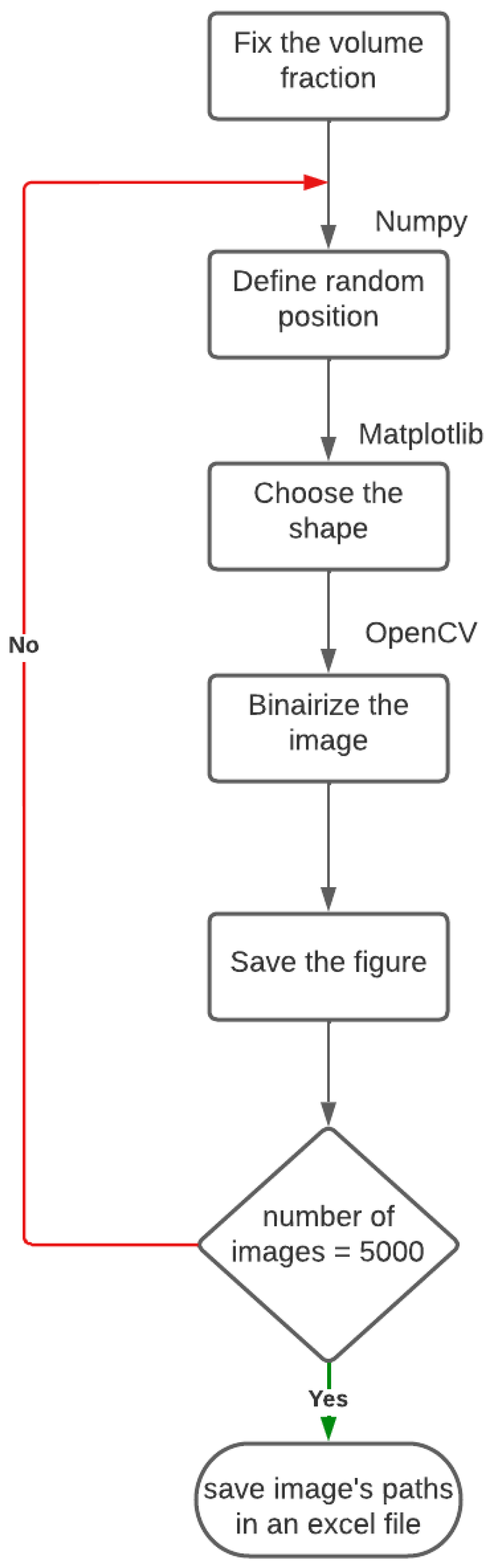
This step consists of collecting the input data, also called Features, which represent in our model the microstructures. In previous studies, the generation of microstructures is always done using Digimat Software, which is software used to generate a Representative Volume Element (RVE) of the great variety of material microstructures. One of the disadvantages of this platform is that it is able to generate only one microstructure per test. In our case, this software would be useless because we needed to run the finite element calculation on a database that contains thousands of 2D images. In order to automate this step, we have developed a python script based on the use of the library Matplotlib and Open CV, capable of generating a huge number of microstructures with different shapes and volume fractions. The algorithm is organized as shown in Figure 1
- -
- Fix the volume fraction by fixing the dimensions of the matrix and the inclusion.
- -
- Define the random position of the inclusion by using the random function of the Numpy library.
- -
- Define the shape of the inclusion by changing the plotting function (Circle, Ellipse, Rectangle…)
- -
- Binarize the image using the THRESH_BINARY function.
- -
- Save the drawn figure.
This algorithm will be put thereafter in a loop whose limits will be fixed according to the number of the microstructure we want to obtain. In our study, we are going to work on databases containing 5000 images each. Each database is divided into 4 sub-bases (1250 images for each shape: circular, elliptical, square, rectangular).
2.2. Finite Element Calculations
The second step consists in collecting the output data, also called Labels, which represent, in our model, the calculated values (bulk, shear, and thermal conductivity).
Specific boundary value problems are used in this study for the determination of isotropic effective elastic properties. More details are given in [21]. To compute effective properties, we choose an elementary volume with imposed macroscopic strain tensors as
An apparent bulk modulus and an apparent shear modulus can be defined as
where is the local stress tensor, is the local shear tensor and < > represents the average on the hole microstructure.
For the thermal problem, the temperature, its gradient, and the heat flux vector are denoted by , and q, respectively. The heat flux vector and the temperature gradient are related using Fourier’s law, which reads
in the isotropic case. The scalar is the thermal conductivity coefficient of the considered phase. A volume V of heterogeneous material is considered again. To compute effective thermal conductivity, the following test temperature gradient, and flux will be prescribed on the elementary volume as
They are used respectively to define the following apparent conductivities:
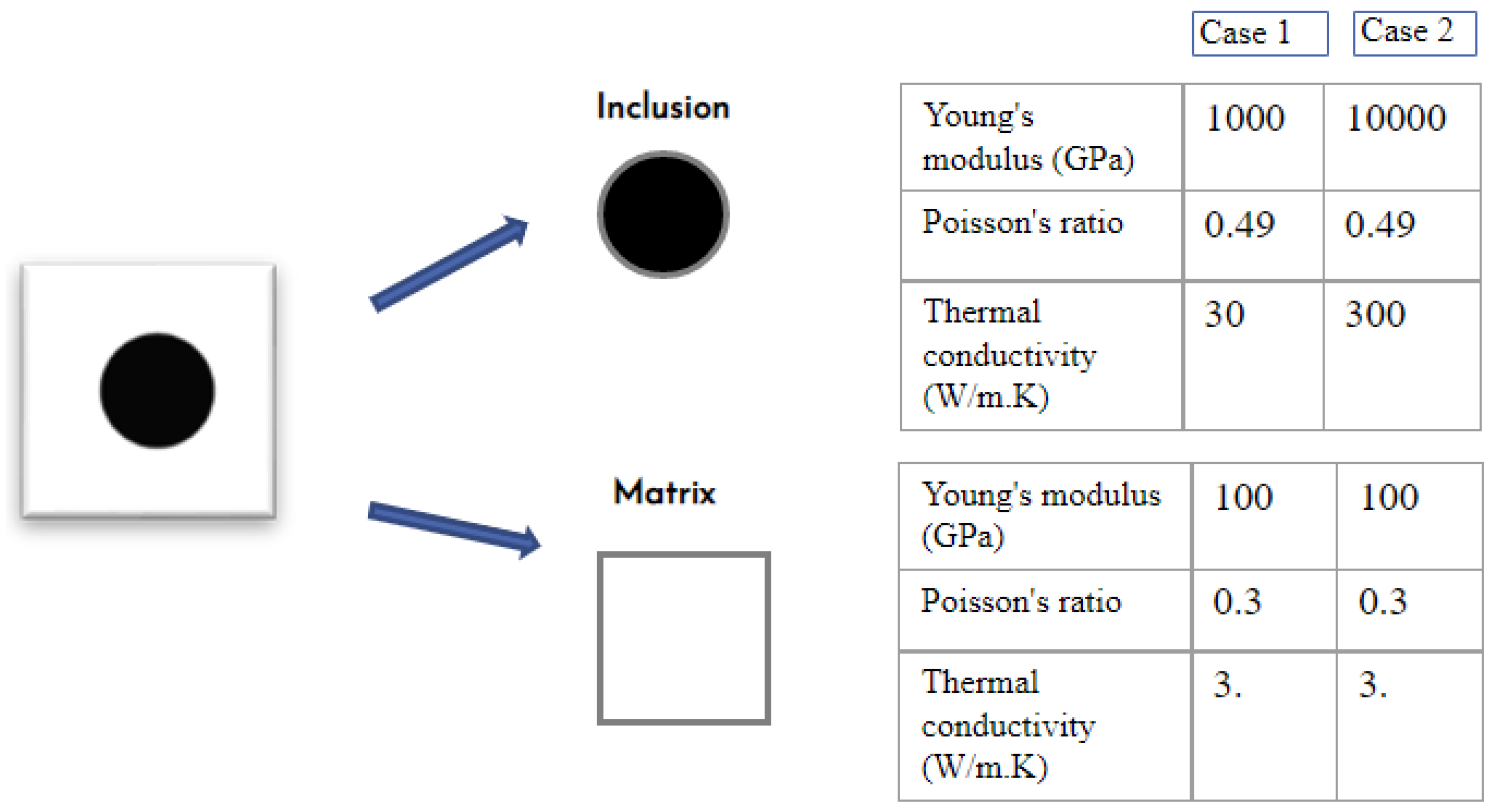
As discussed before, the heterogeneous material used is composed of a matrix and a single inclusion as shown in Figure 2. The value of the volume fraction is modified during the first phase (generation of microstructure), while the value of contrast must be edited in the calculation files before starting the simulations by modifying the value of Young’s modulus as well as the thermal conductivity.
The finite element calculation using the software requires the presence of the following files: a matrix file containing the behaviors of the first phase, an inclusion file containing the behaviors of the second phase, a mesh file, and the input files, in our case we used three files (bulk, shear, and thermal conductivity). Figure 3 shows the elastic and thermal behavior of the different phases.
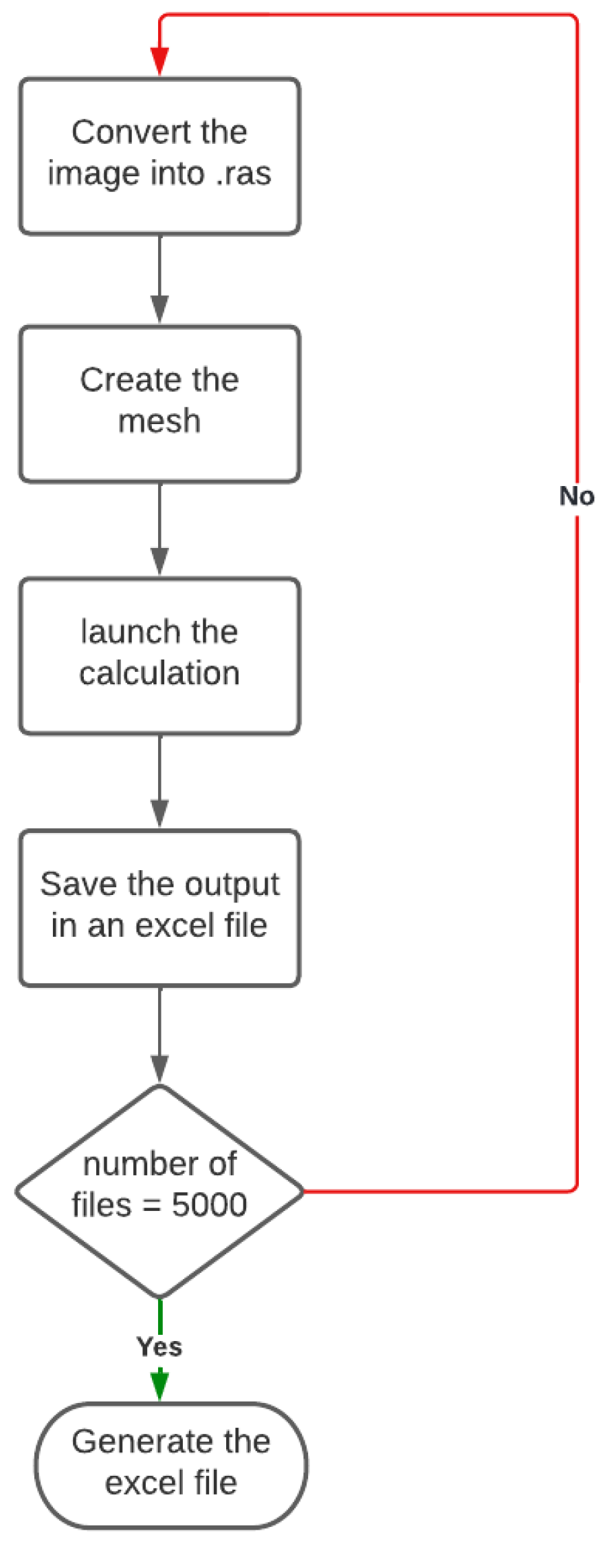
This step is divided into two parts: In the first part, we have developed a shell script able to launch the download and the calculation of different modules on finite element software, the algorithm is organized as shown in Figure 4:
- -
- convert the binary images generated by the first code into “.ras”.
- -
- create the multi-phase mesh.
- -
- launch the calculation to obtain the “.post” file
In the second part, we developed a python script using Data Analysis Library “Pandas” able to generate an excel file of calculated values from calculation files.
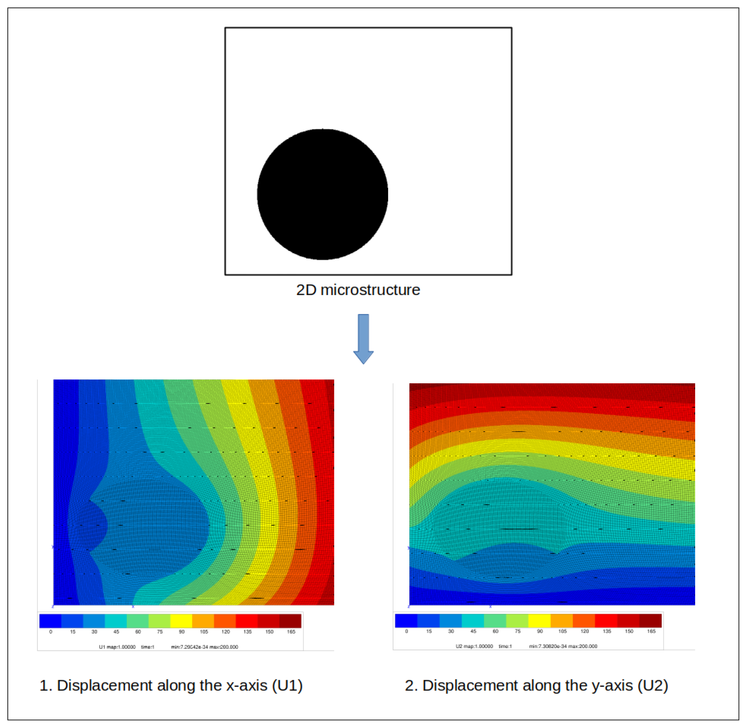
Figure 5 shows an example of a finite element calculation of the bulk modulus based on a 2D morphological image of a composite. It also shows the displacement map in both directions (x and y) using an adequate finite element mesh.
3. Convolutional Neural Network
Convolutional neural networks are a particular form of multi-layer network neurons whose connection architecture is inspired by that of the visual cortex of mammals. They are able to categorize the simplest to the most complex information. They consist of a multi-layer stack of neurons and mathematical functions that pre-process the information before moving on to the hidden computational layers.
3.1. Loading and Pre-Processing Data
In order to predict the behavior of heterogeneous materials, we developed a convolutional neural networks model using Keras and Tensorflow capable of learning from the data set provided without extracting the features. This model takes as input the microstructures converted in binary (matrix in white and inclusion in black). In this first work, we put different shapes of inclusions (circular, elliptical, rectangular, square) by fixing the number of inclusion to 1 and by changing the volume fraction (20%, 25%, 30%) and the contrast between the properties of the inclusion and the matrix (10, 100) in order to have six different databases to work with. The first step is to normalize the input by dividing the pixels of each image by 255. The data will then be divided in a random way into two parts: 80% for the training and 20% for the test.
3.2. CNN Model
The input layer takes 5000 images in total (3200 for model training, 800 for validation, and 1000 for testing). The training data will be filtered through convolution layers using filters, subsequently rectified with the ReLU activation function and reshaped using the max polling operation. The output of the convolutional network will then be the input of the Fully connected where we used three hidden layers before generating the output vector with the flattening operation. Since we work in the case of a regression, the output will be rectified using a linear activation function in order to keep the same output value.
3.2.1. Convolutional Layer
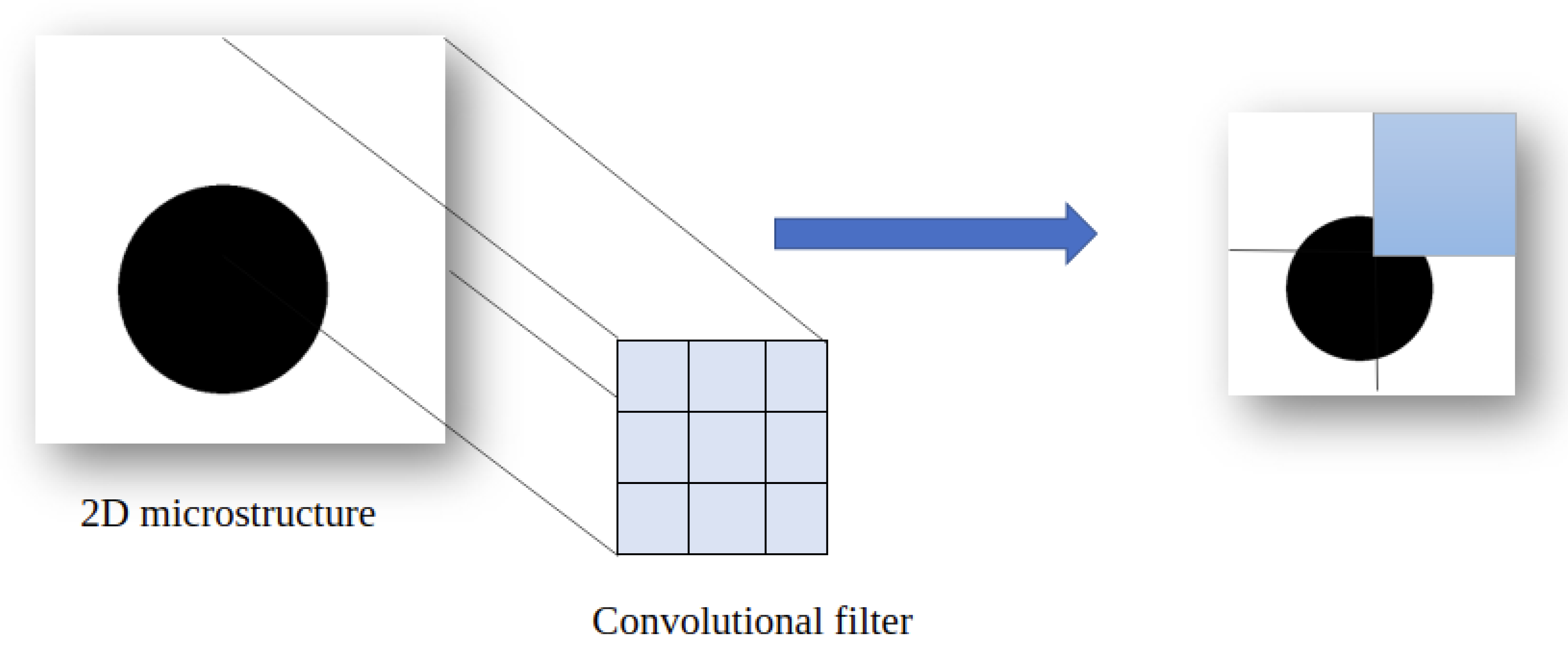
The convolutional layer is the core element of the convolutional neural network. The goal is to detect the most important features by observing the image in its entirety. The convolution layer will focus on each part of the data by analyzing the image by area as shown in Figure 6. In our case, the pattern represents the inclusion; using convolution the model will be able to know the shape and position of the reinforcement in a precise way. The model keeps in memory these characteristics and understands that they represent the selected label. Mathematically speaking, the principle is to drag a window representing the filter on the image and to calculate the convolution product between the filter and each portion of the scanned image. This layer takes as input an image as a 3D tensor and returns what is called a feature-map (also a 3D tensor).
This method is much more efficient than the traditional approach for two main reasons:
- Less error in learning because the model does not learn from images but from features.
- More accuracy in detection, because the model must recognize features and patterns.
When using a convolution layer, we will focus on certain aspects, such as the number of neurons and the size of the pattern. In our model, we have used five convolution layers by doubling the number of neurons (filters) each time, starting with a layer of 16 filters and arriving at the last one containing 256 filters. The size of the extracted pattern is set to pixels for all layers. A first convolution layer (16 filters) will learn small patterns, then the one with 32 filters will learn bigger patterns made of the characteristics of the first layer until we reach the last layer.
3.2.2. Maxpolling Layer
The main idea of Machine Learning is to reduce information to make the data interpretable by the human brain. However, with the layer of convolution used, the amount of information has increased, so it is necessary to reduce the obtained result using Maxpolling operation.
This operation consists in reducing the size of the images while preserving their important features. We obtain the same number of features in output as in input, but they are much smaller. This operation is often placed between two convolution layers, it allows the reduction in the number of parameters and network computation.
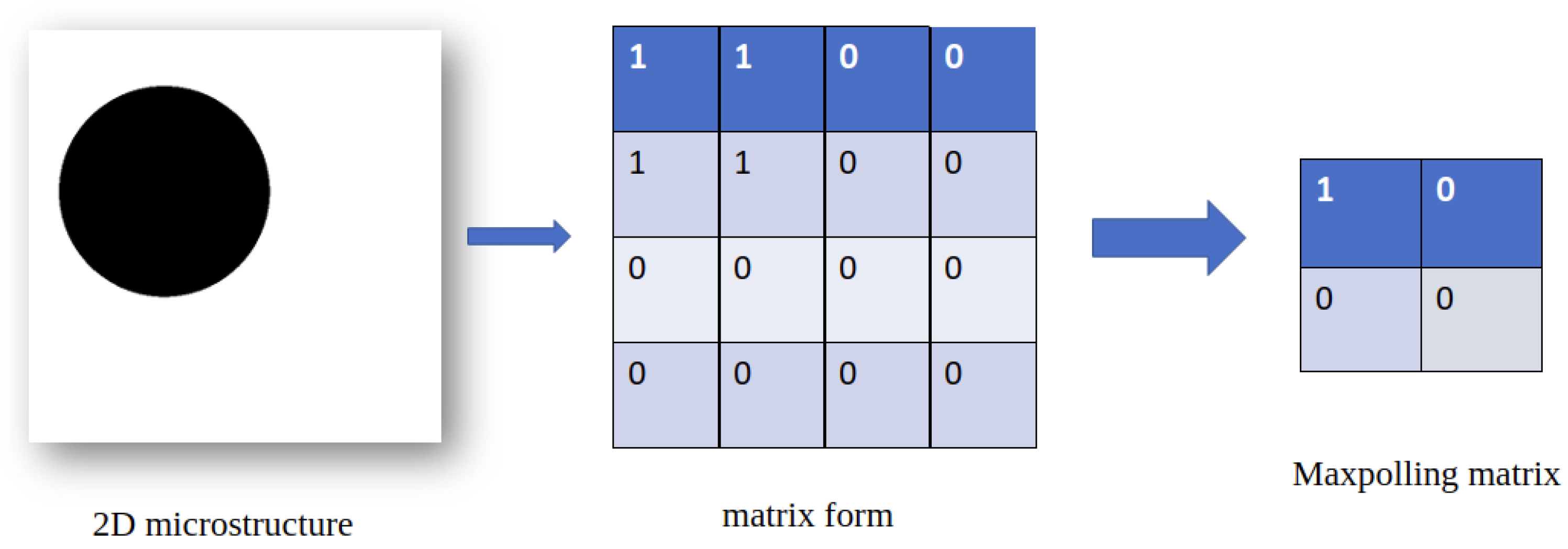
In fact, Maxpooling takes input from feature maps to extract the max value as shown in Figure 7. It keeps only the important information. This allows the Deep Learning model to:
- -
- gain in accuracy by keeping only relevant data.
- -
- gain in speed: the learning of the model is done much faster because the data is getting progressively smaller.
This layer takes as a parameter the kernel size. In our work, the size is fixed to 2 × 2, the dimensions of the image will be divided by 2 after each pooling operation.
3.2.3. Flatten Layer
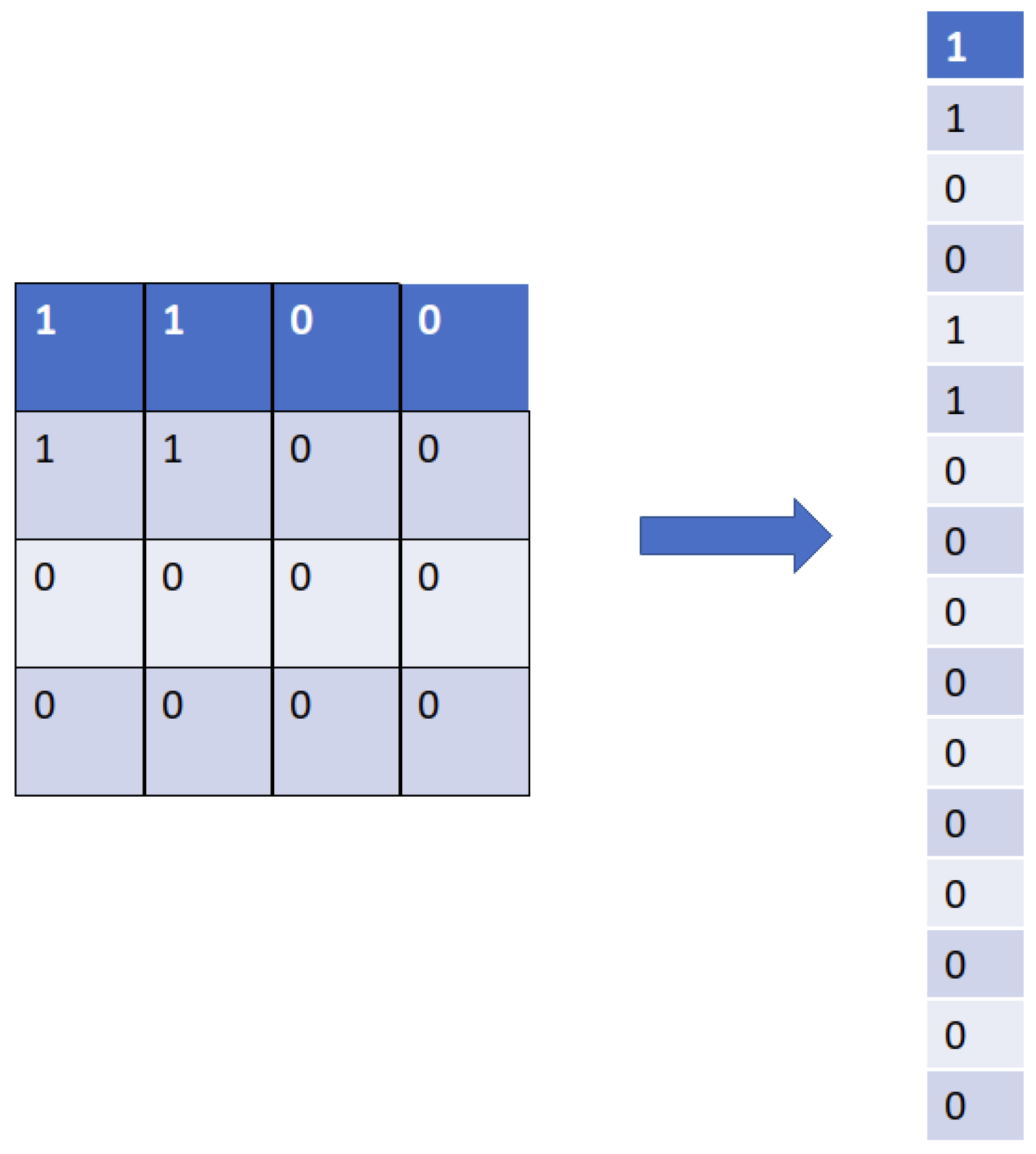
The goal of image processing using neural network technology is to obtain an output label from an input image. For example, in our study, we will give a microstructure as input to obtain the elastic and thermal properties as output, except that the output from the convolution operation, as well as the maxpolling, is a 3 dimensional tensor (height, width, color), which cannot be a final layer. Therefore, we use a layer called Flatten layer which allows the compressing of the tensor to reduce its dimension. It takes as input a 3D tensor and returns a vector. The pixels are recovered line by line and added to the final vector. The example is shown in Figure 8.
3.2.4. Activation Layer
The activation function is an essential element in the creation of a neural network, which is used to modify the data in a non-linear way. This non-linearity allows changing the data representation, which is not possible with a linear transformation. Several types of activation functions exist, such as the sigmoid function used in binary classification [22] or the softmax function for multi-class problems. In order to choose the right activation function, it is necessary to know the direct transformation applied to the data but also its derivative, which will be used in the retro-propagation in order to adjust the values of the weights.
In our model, two activation functions are used:
- The ReLU Function
Its equation is defined by:
The derivative is defined as:
As the convolution performs addition and multiplication operations, the generated values are linear with respect to the input ones, but in an image, the linearity is not very important. So the ReLU function will rectify the values by breaking part of the linearity and therefore allows the acceleration of the calculation. This function will be used after each convolutional layer.
- The Linear Function
The linear function has an equation similar to that of a linear line:
Our research consists in predicting numerical values, so it is a linear regression problem since the output units will be identical to their input level. Hence a linear activation function will be applied at the last hidden layer.
3.3. Compiling and Training
The compilation of the model represents the last step for the model creation that is used to predict the best optimization decisions, by setting these three parameters.
The optimizer controls the learning rate, i.e., the speed at which the optimal weights are computed. The lower the rate, the more accurate the weights, but the longer the learning time. In our case, we will use “Adam,” which is generally the best optimizer to use in order to adjust the learning rate throughout the training.
Adam optimizer involves a combination of two gradient descent methodologies
Momentum is used to speed up the gradient descent algorithm by taking into account the “exponentially weighted average” of the gradients. The use of averages makes the algorithm converge to the minimal value at a faster rate as
where
- mt: aggregate of gradients at time t [current] (initially, mt = 0)
- mt − 1: aggregate of gradients at time t − 1 [previous]
- wt: weights at time t
- wt + 1: weights at time + 1
- t: learning rate at time t
- δL: derivative of Loss Function
- δwt: derivative of weights at time t
- : Moving average parameter (const, 0.9).
Root Mean Square Propagation (RMSP) is an adaptive learning algorithm that seeks to upgrade AdaGrad. Instead of considering the cumulative sum of the squared gradients like in AdaGrad, it considers the “exponential moving average” like:
where
- : weights at time t
- : weights at time
- : learning rate at time t
- δL: derivative of Loss Function
- δ: derivative of weights at time t
- : sum of square of past gradients. [i.e., sum (δL/δ)] (initially, v = 0)
- : Moving average parameter (const, 0.9)
- : A small positive constant ().
The results of the Adam optimizer are generally better than every other optimization algorithm, have a faster computation time, and require fewer parameters for tuning. Because of all that, Adam is recommended as the default optimizer for most of the applications.
The Loss Function is used to find the error or the difference between the predicted value and the true value in the learning process. To develop our model, we chose Mean Absolute Percentage Error (MAPE), which presents the most common choice for regression. The more its value is minimal, the better the model works, its equation is defined as
where
- n is the number of fitted points.
- is the actual value.
- is the predicted value.
Metrics: It is a parameter used to evaluate the performance of the model, similar to the loss function, but not used during the training process. In our model, we have chosen the Mean Absolute Error (MAE). It is a metric used to measure the accuracy of the model as
where
- n is the number of fitted points.
- is the actual value.
- is the predicted value.
The model will be trained by using the function fit(). The main objective of this function is the evaluation of the model during the training. It takes as parameters
- -
- The training data (train_X), the target data (train_y).
- -
- The validation data.
- -
- Epochs: the number of times the model will run the data. The more epochs we run, the more the model will improve up to a certain point. After this point, the model will stop improving at each epoch.
In our model, the training data present, the generated microstructure, and the targets are bulk, shear, and thermal conductivity modulus. The number of epochs is fixed at 30. It means that we will divide the entire data set into 30 small batches.
3.4. Evaluation and Prediction
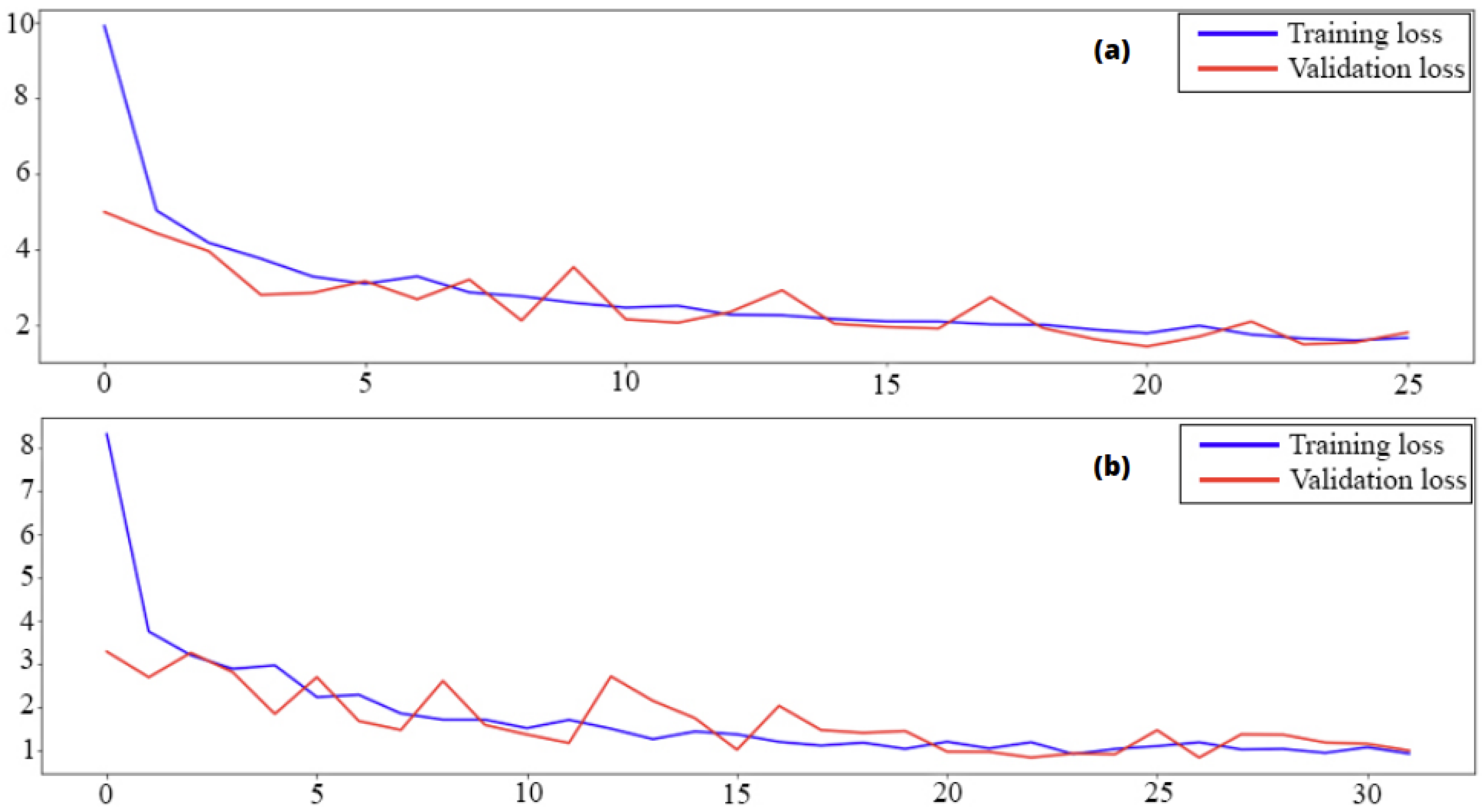
The model evaluation consists of following the evolution of the loss function and the metrics according to the number of epochs. As mentioned at the beginning of this paper, the developed deep learning model will be trained and evaluated using six different databases, and, therefore, we obtain eighteen curves for each parameter. That’s why we will present only two curves, the best one (scenario 4) and the worst one (scenario 6). The fact that the model gives a better score for scenario 4 does not mean that it only performs well in the case of low fractions. For example, the prediction score for scenario 3 (30%) is 95% while that of scenario 1 is 93.3% (20%).
Figure 9 below represents the loss function, i.e., the average absolute percentage of error. The blue curve shows the training data starting from a high value due to the random choice of weights and decreasing during the training until reaching its minimum value.
The other one in red shows the prediction error on the data used for model validation, which starts from a low value and tends towards the same minimum value as the first curve.
The error function converges towards a value included between 0.88% and 0.96%, which explains the efficiency of our model.
This fast convergence is due to the presence of convolutional layers, which consists in analyzing and processing the images in order to facilitate the calculations which will be done by hidden layers. Thanks to feature extraction, the model was able to find the right weight values in 30 epochs.
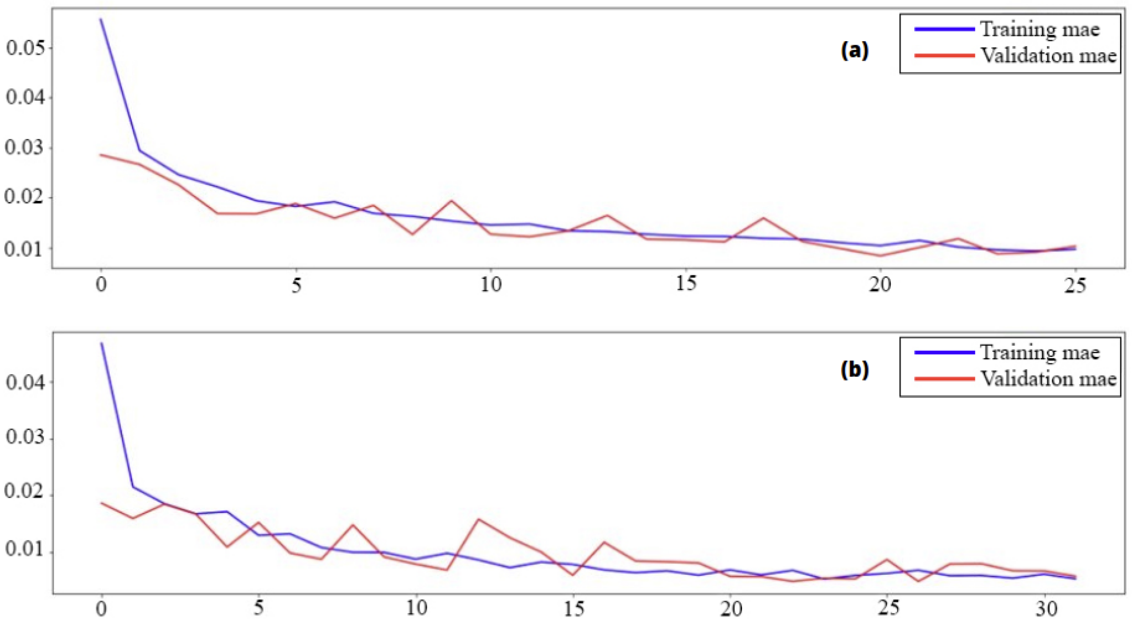
The second one represents the metrics, that is to say, the Mean Absolute Error, as shown in Figure 10.
This metric allows us to measure the average amplitude of the errors in a set of predictions. We can notice from the figure that the training curve, as well as the validation curve, tends to a minimum value close to zero, which shows the small difference between the true values and those predicted.
The MAE presents another method of evaluation. It has the same curve shape as the MAPE but not the same convergence values.
This is the final step and the expected result of the model generation. It consists in applying the prediction model on the test data set and then comparing the output and the true value of shear and bulk and thermal modulus in order to calculate the coefficient of determination as
where:
- is the actual value.
- is the predicted value.
Pearson’s linear coefficient of determination, noted , is a measure of the quality of the prediction of a linear regression.
By testing our model on the 1000 test images generated at the beginning for each database, we obtained a score between 0.92 and 0.97, inclusive, which justifies the good choice of model parameters.
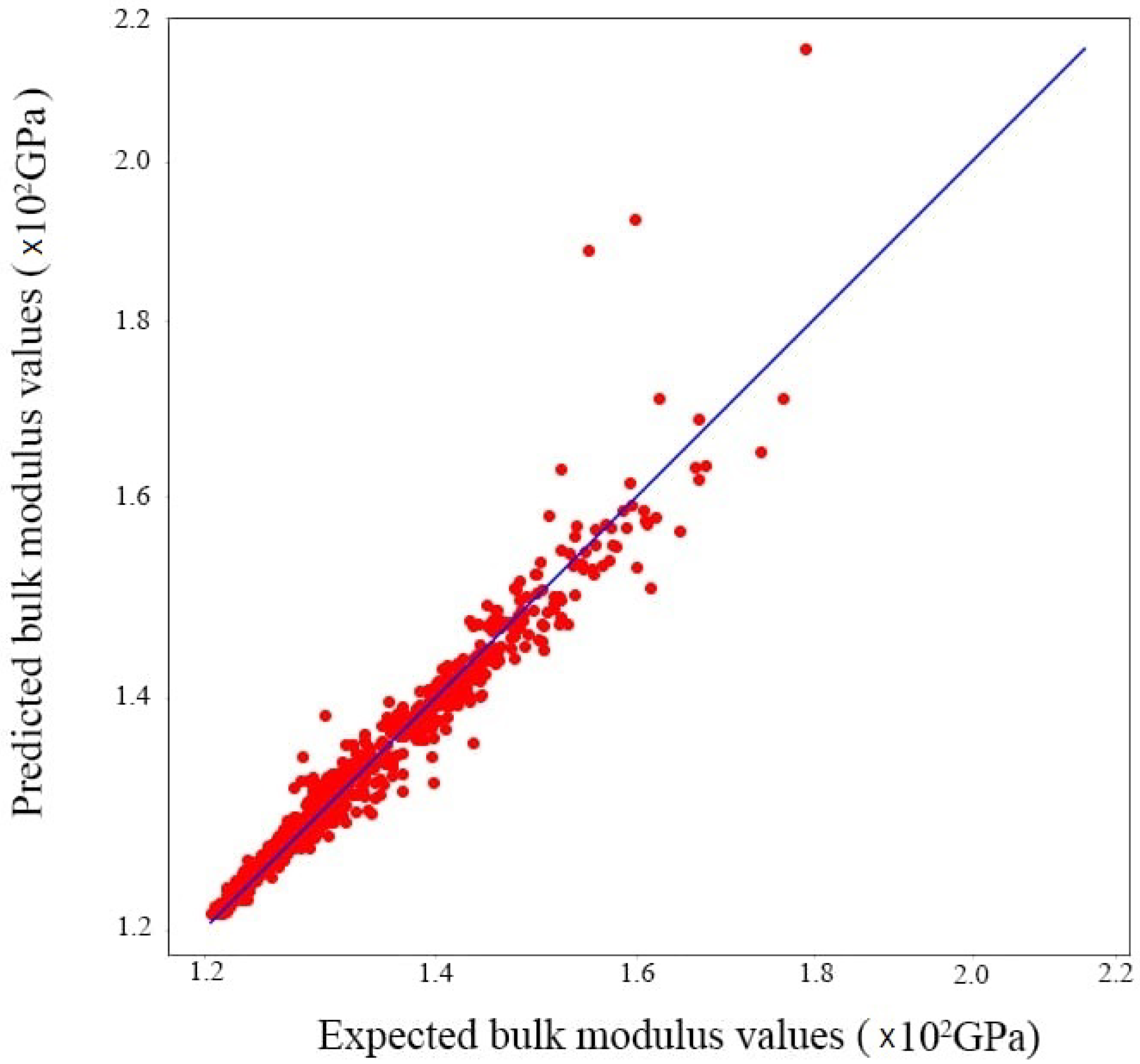
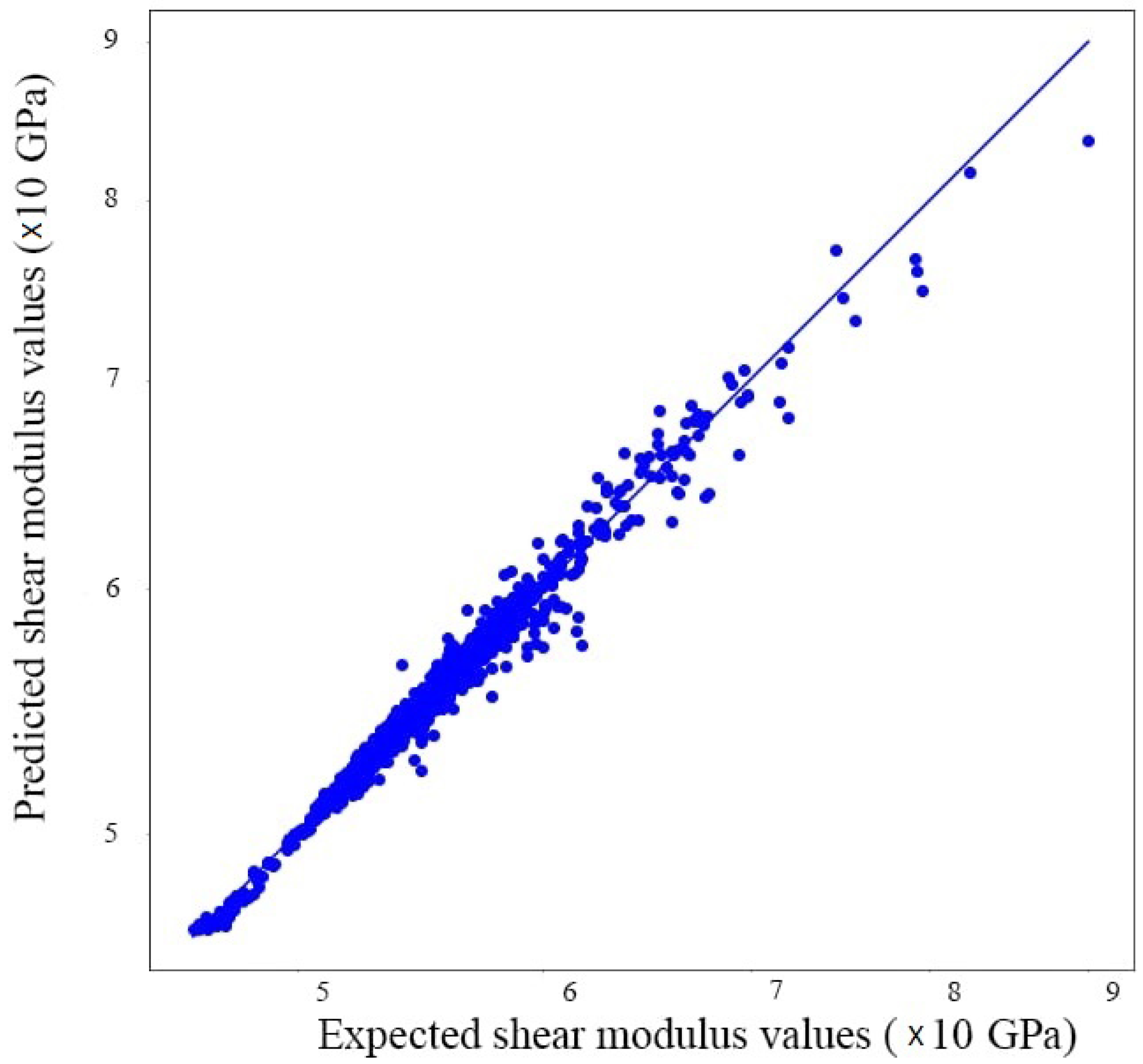
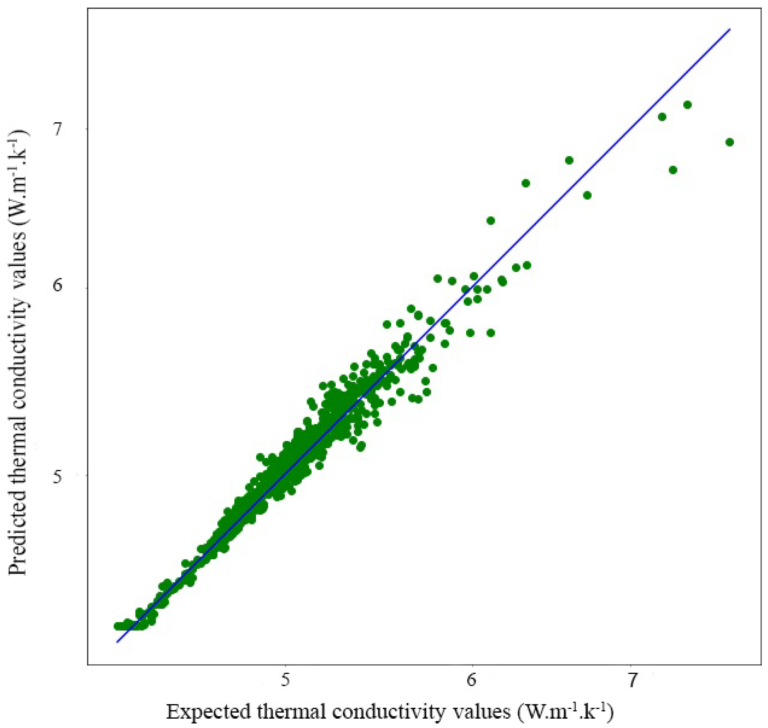
In order to visualize the prediction results, regression curves have been drawn to better explain the phenomenon. Linear regression consists in determining a line or a surface that reduces the differences between the predicted and actual output values. The y-axis shows the model’s predicted values. While the x-axis shows the data set’s actual values. The estimated regression line is the diagonal line in the center of the plot.
Figure 11, Figure 12 and Figure 13 show the results of predictions of different values of modulus (bulk, shear, thermal conductivity) for the case of scenario 4. We can observe that the linear regression line passes through the maximum of the points. We may conclude that the regression model fits the data reasonably well.
Having a 100% accurate prediction, i.e., an error value equal to zero, is technically impossible. This is exactly the case for the points that are far from the regression line, these points cannot be outliers*, because we have already processed the data from the calculation using feature engineering methods such as IQR* and Z score*. Therefore, these points can only be prediction faults, i.e., situations that are a bit difficult for the model, but this does not prevent us from mentioning that the prediction results are excellent, which is well shown by the R score.
- -
- Outliers*: a data which does not ”fit in” with the rest of the data that we are analysing.
- -
- IQR*: the interquartile range, it’s the measure of statistical dispersion equal to the difference between 25% and 75% percentile.
- -
- Z-score*: a tool capable of re-scaling data, its value is between and 3 in the most cases.
In our case, the CNN is the most efficient type of network. The prediction results we found are almost impossible to obtain using other machine learning algorithms like decision trees or random forests or even using an ANN. The advantage of this type of network is that it includes an image processing step before proceeding to prediction. The image goes through convolution, maxpolling, and flattening layers before going to the computation layer. This method is used to reduce the memory footprint and allows for translation invariance processing and therefore improve model performance and increase prediction score.
The aim of the proposed work is not to compare the prediction results of different volume fractions; the main task is to build a machine learning model able to handle all possible cases (different shapes and volume fractions) without using experimental tests or numerical calculations. Through this model, we are able to know the elastic and thermal behavior of a heterogeneous material in a few seconds through its microstructure by referring to the collected database without being obliged to launch calculations on software that can take hours and sometimes days to be done.
4. Conclusions
Through this article, we tested a new method of homogenization based on convolutional neural networks that will allow us to save time and resources compared to other approaches (numerical, analytical). The process of model construction consists first of all in collecting the microstructures by changing the shape and position of the inclusions, the contrast, as well as the volume fraction, and then calculating the different modulus (bulk, shear, thermal conductivity) using finite element homogenization. At the end, the collected database will be trained and tested on our model, which is divided into two parts: a convolutional network that processes the images to facilitate the calculations and a hidden layer network that will, in the end, provide us with the predicted values.
The results obtained demonstrate the appropriate choice of model parameters as well as the efficiency of the operations used in the image processing step.
In this work, we tested the convolutional neural network technology on 2D virtual microstructures with a single inclusion and different shapes in the elastic linear case and the thermal conductivity case. In the next work, we will test 2D and 3D microstructures with more complicated RVE; additionally, we will move away from Hooke’s law by working in the plastic domain.
Author Contributions
Methodology, T.K. and T.M.; writing—original draft preparation, H.B.; writing—review and editing, H.B., T.K. and T.M.; supervision, T.K. and T.M.; simulations, H.B. All authors have read and agreed to the published version of the manuscript.
Funding
This research received no external funding.
Data Availability Statement
Not applicable.
Conflicts of Interest
The authors declare no conflict of interest.
References
- Moumen, A.E. Prévision du Comportement des Matériaux Hétérogènes Basée sur l’Homogénéisation Numérique: Modélisation, Visualisation et Étude Morphologique. Ph.D. Thesis, IBN Zohr University, Agadir, Marocco, 2014. [Google Scholar]
- Kováčik, J.; Simančík, F. Aluminium foam—Modulus of elasticity and electrical conductivity according to percolation theory. Scr. Mater. 1998, 39, 239–246. [Google Scholar] [CrossRef]
- Ding, Y. Analyse Morphologique de la Microstructure 3D de Réfractaires Électrofondus à Très Haute Teneur en Zircone: Relations Avec les Propriétés Mécaniques, Chimiques et le Comportement Pendant la Transformation Quadratique-Monoclinique. Ph.D. Thesis, Ecole Nationale Supérieure des Mines de Paris, Paris, France, 2012. [Google Scholar]
- Zhou, Q.; Zhang, H.W.; Zheng, Y.G. A homogenization technique for heat transfer in periodic granular materials. Adv. Powder Technol. 2012, 23, 104–114. [Google Scholar] [CrossRef]
- Chaboche, J. Le Concept de Contrainte Effective Appliqué à l’Élasticité et à la Viscoplasticité en Présence d’un Endommagement Anisotrope. In Mechanical Behavior of Aniotropic Solids; Springer: Dordrecht, The Netherlands, 1982. [Google Scholar] [CrossRef]
- Wu, T.; Temizer, I.; Wriggers, P. Computational thermal homogenization of concrete. Cem. Concr. Compos. 2013, 35, 59–70. [Google Scholar] [CrossRef]
- Kanit, T.; N’guyen, F.; Forest, S.; Jeulin, D.; Reed, M.; Singleton, S. Apparent and effective physical properties of heterogeneous materials: Representativity of samples of two materials from food industry. Comput. Methods Appl. Mech. Eng. 2006, 195, 3960–3982. [Google Scholar] [CrossRef]
- González, C.; Segurado, J.; Llorca, J. Numerical simulation of elasto-plastic deformation of composites: Evolution of stress microfields and implications for homogenization models. J. Mech. Phys. Solids 2004, 52, 1573–1593. [Google Scholar] [CrossRef]
- Liu, X.; Tian, S.; Tao, F.; Yu, W. A review of artificial neural networks in the constitutive modeling of composite materials. Compos. Part B Eng. 2021, 224, 109152. [Google Scholar] [CrossRef]
- Mentges, N.; Dashtbozorg, B.; Mirkhalaf, S.M. A micromechanics-based artificial neural networks model for elastic properties of short fiber composites. Compos. Part B Eng. 2021, 213, 108736. [Google Scholar] [CrossRef]
- Li, B.; Zhuang, X. Multiscale computation on feedforward neural network and recurrent neural network. Front. Struct. Civ. Eng. 2020, 14, 1285–1298. [Google Scholar] [CrossRef]
- Ford, E.; Maneparambil, K.; Rajan, S.; Neithalath, N. Machine learning-based accelerated property prediction of two-phase materials using microstructural descriptors and finite element analysis. Comput. Mater. Sci. 2021, 191, 110328. [Google Scholar] [CrossRef]
- Minfei, L.; Yidong, G.; Ze, C.; Zhi, W.; Erik, S.; Branko, Š. Microstructure-informed deep convolutional neural network for predicting short-term creep modulus of cement paste. Cem. Concr. Res. 2022, 152, 106681. [Google Scholar] [CrossRef]
- Sun, Z.; Lei, Z.; Zou, J.; Bai, R.; Jiang, H.; Yan, C. Prediction of failure behavior of composite hat-stiffened panels under in-plane shear using artificial neural network. Compos. Struct. 2021, 272, 114238. [Google Scholar] [CrossRef]
- Barbosa, A.; Upadhyaya, P.; Iype, E. Neural network for mechanical property estimation of multilayered laminate composite. Mater. Today Proc. 2020, 28, 982–985. [Google Scholar] [CrossRef]
- Kim, D.W.; Lim, J.H.; Lee, S. Prediction and validation of the transverse mechanical behavior of unidirectional composites considering interfacial debonding through convolutional neural networks. Compos. Part B Eng. 2021, 225, 109314. [Google Scholar] [CrossRef]
- Venkatesan, N. An Introduction to Making Scientific Publication Plots with Python. Available online: https://towardsdatascience.com/an-introduction-to-making-scientific-publication-plots-with-python-ea19dfa7f51e (accessed on 2 February 2023).
- Gregori, E. Introduction To Computer Vision Using OpenCV. Presented at the 2012 Embedded Systems Conference, San Jose, CA, USA, 26–29 March 2011. [Google Scholar]
- Tanner, G. Introduction to Deep Learning with Keras. 2019. Available online: https://gilberttanner.com/blog/introduction-to-deep-learning-withkeras/ (accessed on 2 February 2023).
- Abadi, M.; Barham, P.; Chen, J.; Chen, Z.; Davis, A.; Dean, J.; Devin, M.; Ghemawat, S.; Irving, G.; Isard, M.; et al. TensorFlow: A System for Large-Scale Machine Learning. In Proceedings of the 12th USENIX Symposium on Operating Systems Design and Implementation (OSDI ‘16), Savannah, GA, USA, 2–4 November 2016. Section: GBlog. [Google Scholar]
- Kanit, T.; Forest, S.; Galliet, I.; Mounoury, V.; Jeulin, D. Determination of the size of the representative volume element for random composites: Statistical and numerical approach. Int. J. Solids Struct. 2003, 40, 3647–3679. [Google Scholar] [CrossRef]
- Rogala, T.; Przystałka, P.; Katunin, A. Damage classification in composite structures based on X-ray computed tomography scans using features evaluation and deep neural networks. Procedia Struct. Integr. 2022, 37, 187–194. [Google Scholar] [CrossRef]
Figure 1.
Descriptive flowchart of the data collection process through a python script based on the use of Matplotlib and OpenCV.
Figure 1.
Descriptive flowchart of the data collection process through a python script based on the use of Matplotlib and OpenCV.

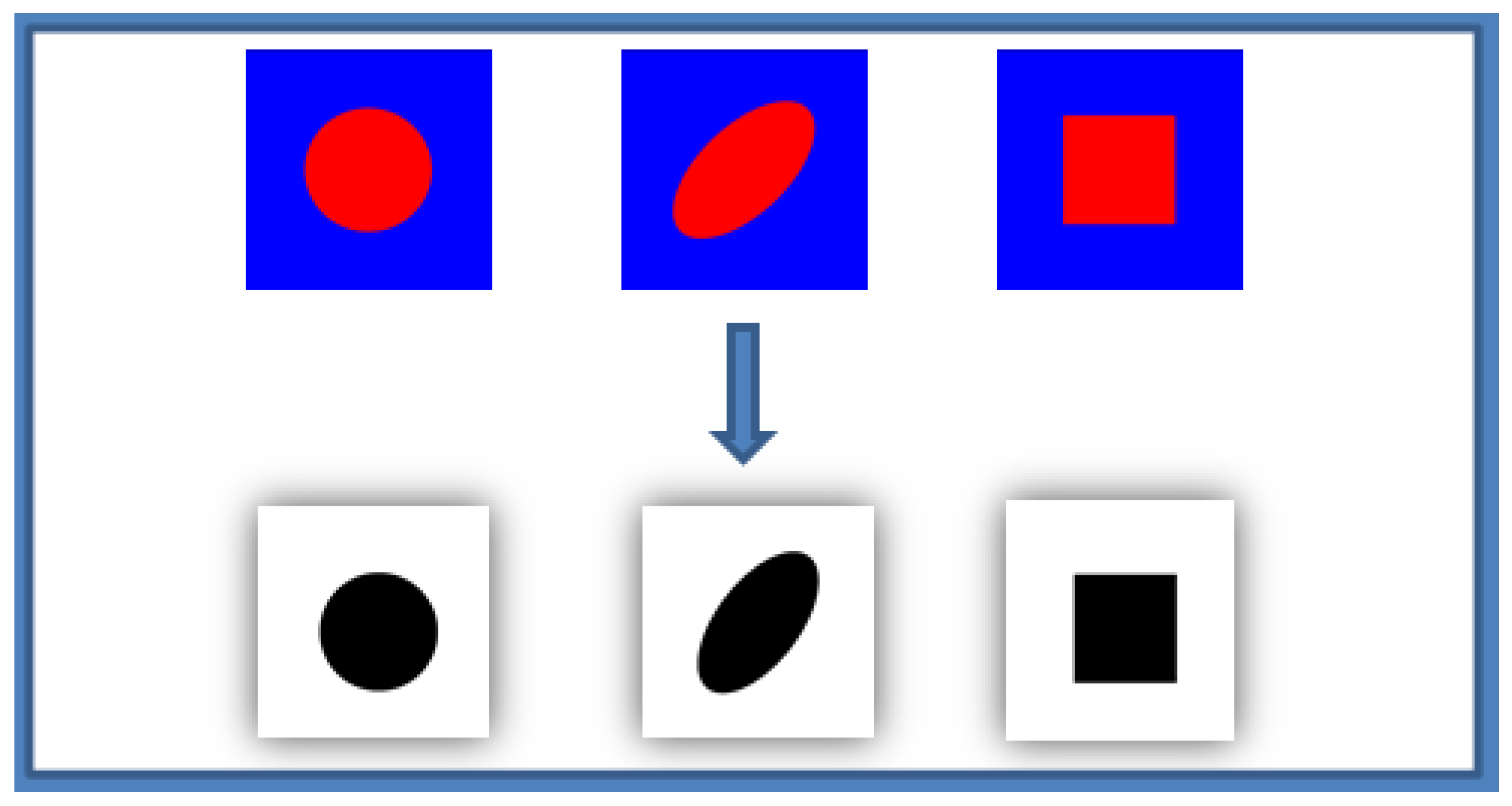
Figure 2.
Binarization of the different microstructure images with a different shape and a fixed volume fraction (30%) using THRESH_BINARY function of OpenCV library.
Figure 2.
Binarization of the different microstructure images with a different shape and a fixed volume fraction (30%) using THRESH_BINARY function of OpenCV library.

Figure 3.
The elastic (Young modulus) and thermal (Thermal conductivity) properties of two different material phases (the values in the table are not realistic, just used for the calculation).
Figure 3.
The elastic (Young modulus) and thermal (Thermal conductivity) properties of two different material phases (the values in the table are not realistic, just used for the calculation).

Figure 4.
Descriptive flowchart of the output collection process based on the use of finite element software.
Figure 4.
Descriptive flowchart of the output collection process based on the use of finite element software.

Figure 5.
Example of a finite element calculation of the bulk modulus based on a 2D morphological image of a composite.
Figure 5.
Example of a finite element calculation of the bulk modulus based on a 2D morphological image of a composite.

Figure 6.
Detection of the important features of the 2D microstructure using the different filters of convolutional layer.
Figure 6.
Detection of the important features of the 2D microstructure using the different filters of convolutional layer.

Figure 7.
Reduction of the image shape using polling operation consists at extracting the maximum value from each sub-matrix.
Figure 7.
Reduction of the image shape using polling operation consists at extracting the maximum value from each sub-matrix.

Figure 8.
Transformation of the output matrix into a vector using flattening by recovering the pixels line by line and adding them to the final vector.
Figure 8.
Transformation of the output matrix into a vector using flattening by recovering the pixels line by line and adding them to the final vector.

Figure 9.
Mean Absolute Percentage Error curves using training and validation data consists in following the evolution of the training according to the number of epochs, (a) presents scenario 4 while (b) presents scenario 6.
Figure 9.
Mean Absolute Percentage Error curves using training and validation data consists in following the evolution of the training according to the number of epochs, (a) presents scenario 4 while (b) presents scenario 6.

Figure 10.
Mean Absolute Error curves using training and validation data consists in following the evolution of the training according to the number of epochs, (a) presents scenario 4 while (b) presents scenario 6.
Figure 10.
Mean Absolute Error curves using training and validation data consists in following the evolution of the training according to the number of epochs, (a) presents scenario 4 while (b) presents scenario 6.

Figure 11.
Convolutional predictions for the bulk modulus.

Figure 12.
Convolutional predictions for the shear modulus.

Figure 13.
Convolutional predictions for the thermal conductivity.


Table 1.
The 6 different calculation scenarios to be tested, collected by modifying the contrast and the volume fraction.
Table 1.
The 6 different calculation scenarios to be tested, collected by modifying the contrast and the volume fraction.
| Scenarios | Contrast | Volume Fraction |
|---|---|---|
| Scenario 1 | 20% | |
| Scenario 2 | 10 | 25% |
| Scenario 3 | 30% | |
| Scenario 4 | 20% | |
| Scenario 5 | 100 | 25% |
| Scenario 6 | 30% |
Disclaimer/Publisher’s Note: The statements, opinions and data contained in all publications are solely those of the individual author(s) and contributor(s) and not of MDPI and/or the editor(s). MDPI and/or the editor(s) disclaim responsibility for any injury to people or property resulting from any ideas, methods, instructions or products referred to in the content. |
© 2023 by the authors. Licensee MDPI, Basel, Switzerland. This article is an open access article distributed under the terms and conditions of the Creative Commons Attribution (CC BY) license (https://creativecommons.org/licenses/by/4.0/).
Share and Cite
MDPI and ACS Style
Béji, H.; Kanit, T.; Messager, T. Prediction of Effective Elastic and Thermal Properties of Heterogeneous Materials Using Convolutional Neural Networks. Appl. Mech. 2023, 4, 287-303. https://doi.org/10.3390/applmech4010016
AMA Style
Béji H, Kanit T, Messager T. Prediction of Effective Elastic and Thermal Properties of Heterogeneous Materials Using Convolutional Neural Networks. Applied Mechanics. 2023; 4(1):287-303. https://doi.org/10.3390/applmech4010016
Chicago/Turabian StyleBéji, Hamdi, Toufik Kanit, and Tanguy Messager. 2023. "Prediction of Effective Elastic and Thermal Properties of Heterogeneous Materials Using Convolutional Neural Networks" Applied Mechanics 4, no. 1: 287-303. https://doi.org/10.3390/applmech4010016