Euler–Euler Multi-Scale Simulations of Internal Boiling Flow with Conjugated Heat Transfer


PROMES Laboratory, CNRS—University of Perpignan (UPVD), 66100 Perpignan, France
*
Author to whom correspondence should be addressed.
Appl. Mech. 2023, 4(1), 191-209; https://doi.org/10.3390/applmech4010011
Submission received: 30 November 2022
/
Revised: 6 January 2023
/
Accepted: 31 January 2023
/
Published: 6 February 2023
(This article belongs to the Special Issue Applied Thermodynamics: Modern Developments (2nd Volume))
Abstract
:A numerical approach was implemented, to study a boiling flow in a horizontal serpentine tube. A NEPTUNE_CFD two-fluid model was used, to study the behavior of the refrigerant R141b in diabatic cases. The model was based on the Euler–Euler formalism of the Navier–Stokes equations, in which governing equations are solved for both phases of the fluid at each time step. The conjugate heat transfer—between the tube wall and the fluid—was considered via a coupling with the SYRTHES 4.3 software, which solves solid conduction in three dimensions. A mesh convergence study was carried out, which found that a resolution of 40 meshes per diameter was necessary for our case. The approach was validated by comparison with an experimental study of the literature, based on the faithful reproduction of the positions of two-phase flow regime transitions in the domain. Original post-processing was used, to unravel the flow characteristics. The mean and RMS fields of void fraction, temperatures and stream wise velocities in several sections were analyzed, when statistical convergence was reached. A thermal equilibrium was reached in the saturated liquid, but not in the vapor phase, due to the flow dynamic and possibly the presence of droplets. Finally, a thermal analysis of the configuration was proposed. It demonstrated the strong coupling between the temperature distribution in the solid, and the two-phase flow regimes at stake in the fluid domain.
1. Introduction
Two-phase flows are ubiquitous in nature and engineering applications: to name but a few, they are present in many chemicals and energy processes; in particular, they are used in concentrated solar energy conversion processes, also known as solar thermodynamic processes. In the context of this study, we focused on a specific technology: the direct steam generation receiver, as implemented in the Llo solar power plant, in France. The process principle is described in the following.
Sun rays were concentrated to a receiver by use of Fresnel mirrors (heliostats), which imposed an anisotropic wall heat flux on the external surface of stainless steel tubes. Water, which was used as heat transfer fluid, was injected, sub-cooled, at the inlet of a 500 m length tubes. The heat from the wall was transferred to the water by a wall convective exchange. Vapor was then created by nucleate ebullition. The outlet void fraction, which corresponded to the volume fraction of vapor, was managed, so as not to exceed 80%. However, the behavior of the flow inside the tube was still not well characterized: further understanding of these flows could enable improvement of parietal heat transfers, so as to be able to predict the steam production of a solar power plant. Finally, an assessment of thermomechanical stresses in the tubes was also required, to optimize the lifespan of solar receivers. In this context, and as a first step towards solar receiver modeling, the present work focused on the numerical modeling of non-isothermal liquid-vapor two-phase flow in horizontal configurations. The present approach was validated against experimental data available in the literature [1].
Simulating such flows remains a major challenge, although massive efforts have been devoted during the last two decades to develop modeling strategies aimed at computing multiphase flows [2]: these strategies differ according to the level of accuracy they target and the computational resources they require.
The simplest approach to dealing with such a flow pattern is based on the homogeneous model, which considers the flow as a single fluid, the properties of which are a phase average of the properties of the two-phase (thus weighted by the void fraction); however, with this approach, the void fraction is not transported, and the properties of the homogeneous fluid do not depend on the local phase distribution of the two-phase flow in the calculation domain [3]: for this reason, this method was not suitable for studying the regime transition and the evolution of the phase distribution of a two-phase flow.
A natural extension, which has been used extensively for the last two decades, is to solve a transport equation for the volume fraction together with the Navier–Stokes (NS) equations. With such an approach, a precise localization of the interfaces is possible in the computational domain, and enables the imposition an appropriate jump condition across the interface. Three main types of interface tracking techniques are now available in the literature, namely the Volume Of Fluid [4], Level Set [5] and Front Tracking [6] methods (see also [7,8,9] for reviews). These approaches are now mature, and provide insight into a wide range of physical configurations [10,11]: their main limitation lies in their computational cost, which limits their application to academic cases; indeed, in this framework, each inclusion of the two-phase flow must be at least 10 times larger than the characteristic size of the mesh.
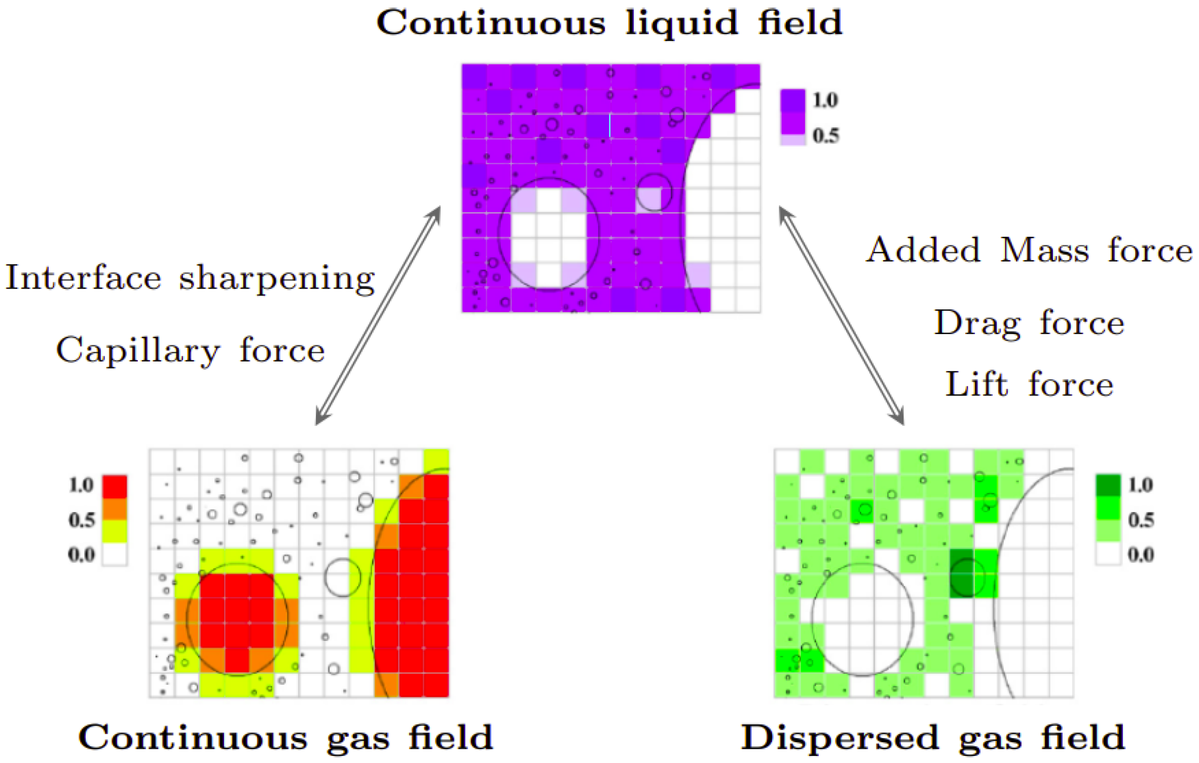
An alternative way to relax the computational cost constraint, for complex geometries that may involve a wide range of two-phase structures, is provided by the Euler–Euler approach, based on the so-called two-fluid model [12,13]: in this approach, the governing equations are obtained by phase-averaging the NS equations, pushing the unknown terms to the interfaces. Closing terms are therefore needed, to model these interfacial coupling terms. The accuracy of the simulations therefore relies on the correctness of the closures. In this framework, NS equations are solved for the liquid phase and for the vapor phase. The validity of the model is based on the ability of interfacial closure laws to properly model interfacial transfers. This method was initially developed to represent dispersed flows [14]. Over the past decade, multi-scale extension has developed, to expand the flow regimes that can be modeled within the Euler–Euler framework [15,16,17,18,19]: in the present study, this last approach was employed, through the NEPTUNE_CFD 6.1 software. The simulations performed in this study relied on a two-field approach, with one field for the vapor phase, and another field for the liquid. The distinction between the continuous vapor field and the dispersed vapor field was made via different closure terms in a GLIM fashion (see Figure 1). Details of the closure terms for the different scales of the gas content are presented in Section 2.2.
The objective of this work was to validate the use of NEPTUNE_CFD software to compute two-phase flows in solar receivers: experimental data from anisothermal flows were thus required to validate the model; however, the literature does not provide experimental data on water-steam flows with phase change in horizontal pipes. Most of the literature concerns vertical two-phase flows [20,21,22]; few experimental studies in horizontal configuration have been carried out [23,24,25] for liquid-vapor or air-water flows. No visualization of the flow had been provided, which was inconvenient for locating regime transitions; however, Yang undertook, in 2008, an experimental study on freon ebullition, providing visualizations of liquid-vapor interface inside the tube [1]: latterly, this work has been used to confront numerical simulations of liquid-vapor two-phase flows on Fluent 14.5 software [26,27]. Due to the lack of experimental data in the literature, this experiment was chosen as a comparative tool to validate the numerical model developed in this work. If the application differed from the one in the solar receivers, the physics inside the tube remained the same, as explained in Section 2.1. As in Dinsenmeyer [26,27], we therefore assessed the suitability of our approach by verifying that it was able to reproduce the regime transitions observed by Yang [1]; however, we proposed an original approach—this case being the first time, to our knowledge—in which we evaluated the mesh convergence of the method, and proposed original post-processing, to unravel the characteristics of the flow and the heat transfers in this setup.
In order to address the aforementioned problem, the rest of the paper is organized as follows: the Yang case is presented in Section 2.1; the modeling approach is detailed in Section 2.2; a brief description of our numerical setup and methods is given in Section 2.3; the main results of this study are presented in Section 3; we first evaluate the convergence of the mesh in Section 3.1; a detailed validation of our approach against Yang’s benchmark case is performed in Section 3.2; the flow patterns are further analyzed, thanks to original data post-processing, in Section 3.3; the robustness of the approach is discussed in Section 3.4 by performing simulations for all the cases presented by Yang; a qualitative thermal analysis of the flow is given in Section 3.5; finally, Section 4 summarizes the main results of the study, and outlines some perspectives.
2. Materials and Method
2.1. Yang’s Reference Case
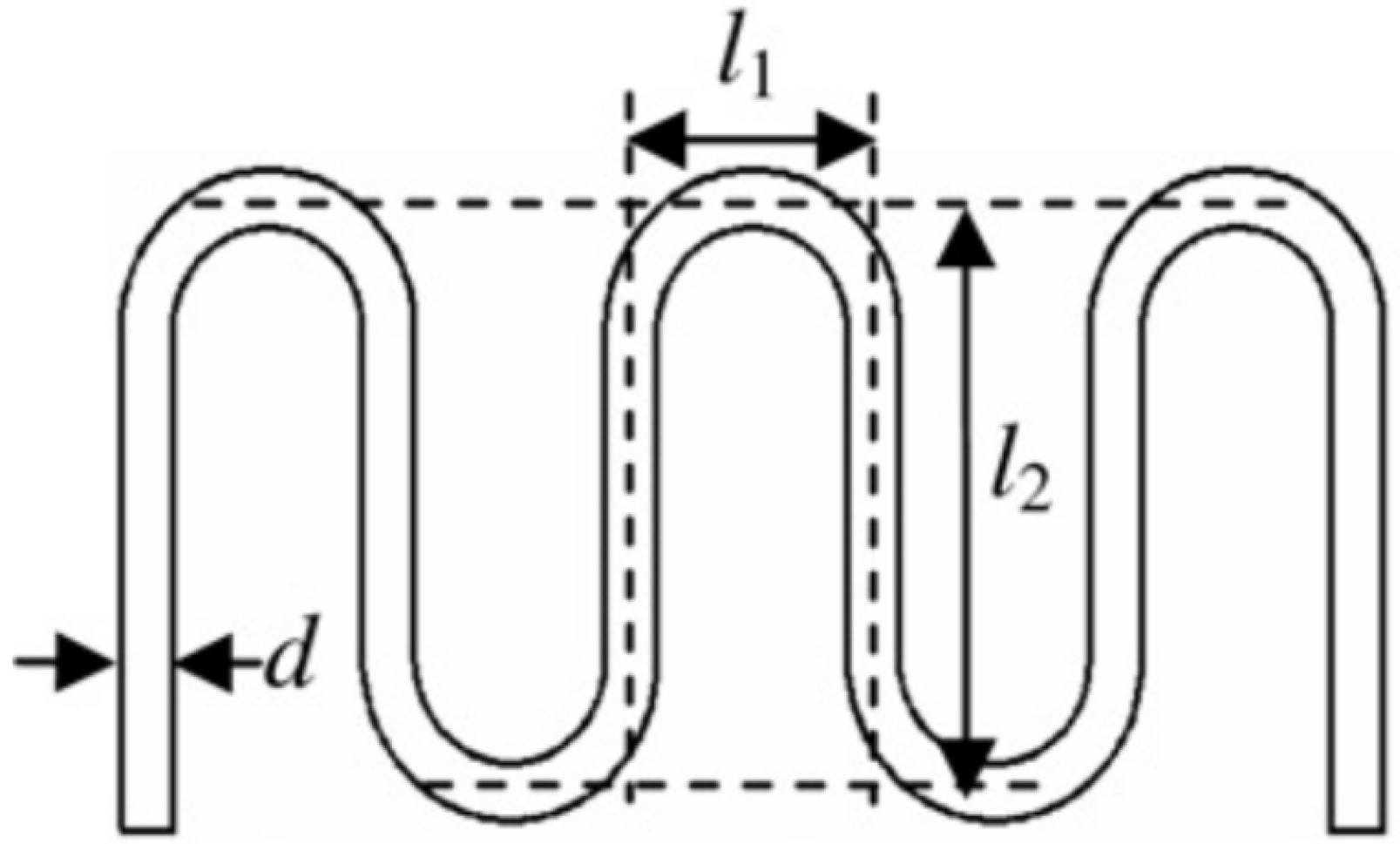
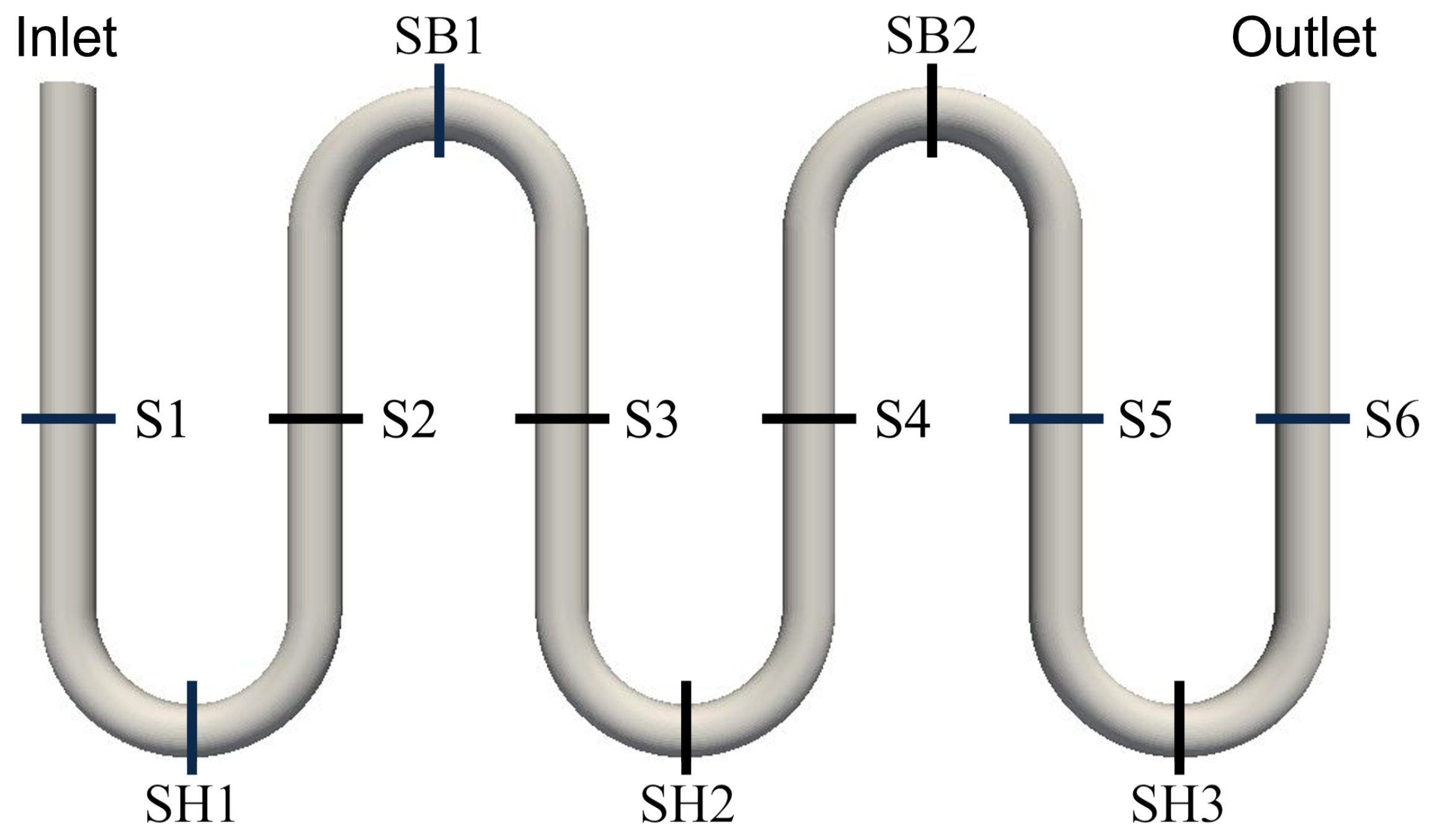
The study was based on a horizontal flow in a serpentine pipe, as presented in Figure 2. The inner diameter of the tube was equal to 6 mm, with a thickness of 1 mm. The lengths identified as and in Figure 2 were equal to 28 mm and 70 mm, respectively, which led to a total unwound length of 504 mm. The tube was made of quartz glass, and coated with a thin layer of an electric conducting metal oxide. The material properties are summarized in Table 1. A voltage difference was applied between two electrodes, which were placed at the inlet and the outlet of the tube. Thereafter, an isotropic heat flux was applied to the external wall, thanks to the Joule effect. The refrigerant R141b was used as heat transfer fluid: its physical properties, which varied with temperature, were extracted from the CoolProp library.
In the experiment, a subcooled liquid phase flow was imposed on the inlet of the tube at a constant mass flow. Due to the heat flux imposed on the wall, a two-phase boiling flow developed along the tube, and various two-phase flow regimes were observed. The different cases presented in the paper, for the various control parameters, show a broad spectrum of two-phase flow regimes (from bubbly to stratified), along with their respective transitions. The different cases provided in the article are summarized in Table 2.
The main differences between this study and a solar receiver are: (i) the presence of elbows in Yang et al.’s study; (ii) the different working fluid (R141b vs. water); (iii) the heat flux distribution (isotropic vs. anisotropic distribution); however, the physics of the flow remained the same as the regimes evolved along the tube, which was why this was an excellent test case for the present study.
Alongside the experiments, Yang et al. also presented CFD calculations of their different cases. The simulations were performed with ANSYS Fluent, using a one-fluid model coupled with the Volume Of Fluid (VOF) method. The domain was divided into 118,000 meshes, which seemed relatively small, based on the calculations carried out in our study. No information was provided on how the heat conduction was resolved in the pipe wall.
2.2. Euler–Euler Boiling Flow Modeling
All the simulations presented in this study were performed using the 6.1 version of NEPTUNE_CFD software, jointly developed by EDF, CEA, IRSN and Framatome for more than a decade. The governing equations considered in this code were based on an extension to n fields of the two-fluid model [13]. Mass, momentum and energy conservation equations were solved for each field. From a numerical point of view, all the governing equations were discretized using a finite volume technique with collocated variables. The grid was unstructured, and involved arbitrarily shaped cells. A second-order linear upwind scheme was used to update the volume fraction of each field. The velocity field was advanced thanks to a fractional step technique, while the pressure field was computed with the help of the SIMPLE algorithm [28]. An iterative coupling between energy and mass balances was used, to enforce the simultaneous conservation of both quantities [29].
2.2.1. Governing Equations
When considering a liquid-vapor two-phase flow, everywhere in the domain, the following condition must be satisfied:
This equation gives information on the phase distribution. When equals 0, then the cell only contains vapor, whereas when , the cell only contains liquid; however, for intermediate values between 0 and 1, it characterizes the presence of a two-phase flow (large interfaces, vapor bubbles, or droplets).
For each phase k, the continuity Equation (2) is written:
where represents the mass transfer from phase p to k:
Necessarily, equals 0.
The momentum equation is described below:
represents the momentum transfer term from phase p to k. The viscous stress tensor is given by Equation (5):
The closure law regarding the interfacial momentum transfer depends on the nature of the phases on both sides of the interface. For an interface between continuous liquid (CL) and dispersed gas (DG), the momentum transfer term reduces to the sum of a drag (), an added mass (), a lift () and turbulent dispersion forces (), as depicted in Equation (6):
For an interface delimiting a CL and continuous gas (CG) phases—hereafter called large interfaces—the closure law must be adapted, to enforce normal velocity continuity at the interface, and to allow the latter to deform itself: to do so, we considered a friction force (), a penalty force () and a capillary force (), as depicted in Equation (7). The reader is referred to [15] for more details on the different modeling options.
Finally, the energy conservation is solved for the total enthalpy, which leads to the formulation given by Equation (8):
With , the energy transfer term at the interface depends on two contributions:
depends on mass transfer, whereas does not depend on the latter.
2.2.2. Wall Boiling Model
Two steps are required to model wall heat flux: (a) the definition of the beginning of boiling; (b) the computation of incident heat flux.
(a) In NEPTUNE_CFD software, the Hsu criteria [30] are implemented, to define the onset of boiling at the wall: this indicates that a bubble will grow in a vapor cavity if the liquid temperature, at the extremity of this cavity, is at least equal to the saturation temperature within the bubble. Vapor is created inside a cavity if the radius of the latter is larger than the activation radius defined by Equation (10):
where is defined as the limit temperature, below which there is no sustained boiling:
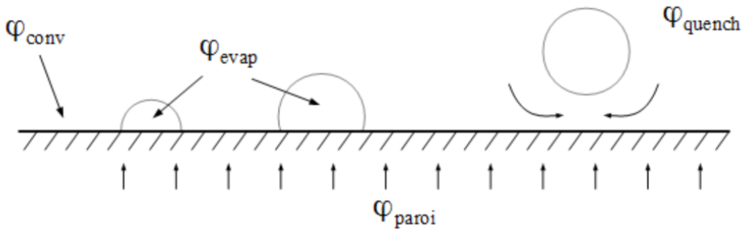
(b) The Kurul and Podowski model [31] is adopted in these simulations, which decomposes the incoming parietal flux into three contributions: a convective flux (), unaffected by the presence of bubbles; a quenching flux (), induced by the cold water brought when bubbles leave the wall; and an evaporation flux, to generate vapor () (see Figure 3).
The quantity of Equation (12) is given by
2.3. Numerical Set up and Methods
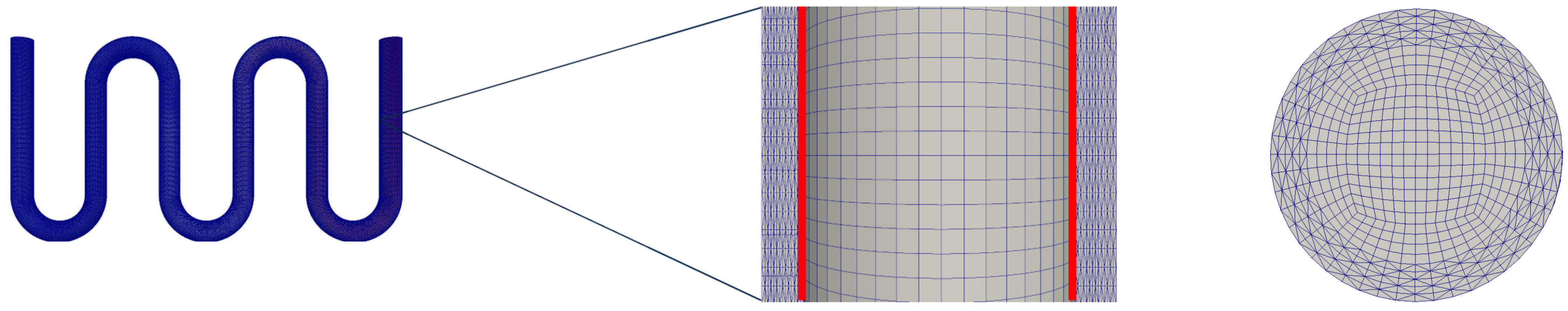
Simulations with conjugated heat transfer were performed with NEPTUNE_CFD software coupled with SYRTHES software, in order to solve 3-dimension conduction in the tube. The surface where the coupling occurred is represented in red on Figure 4. At each time step, the temperature computed by SYRTHES was given to NEPTUNE_CFD for all meshes at the interface between fluid and solid. The pipe thickness was divided into five meshes for all the simulations performed, and the influence of the flow domain resolution on the results was assessed (see Section 3.1). The flow was assumed to be incompressible in each phase. At the interface, the velocity jump was described by the right-hand term of Equation (2). A priori tests have shown that the consideration of a turbulence model has no significant influence on the results; therefore, for the sake of numerical cost, the simulations presented in this study were obtained without any turbulence model in the flow core. Heat losses by natural convection were considered on the external surface of the serpentine pipe, considering an ambient temperature of : we estimated the latter, as the authors did not provide this information in their paper. The convective heat transfer coefficient was estimated by the correlation of Churchill and Chu [33].
The boundary conditions were set as follows: at the inlet, the fluid was injected, sub-cooled between or , depending on the case, while the atmospheric pressure was imposed at the outlet; wall heat flux was applied to the external surface of the pipe; in all the simulations, the fluid and thermal conditions were those defined by Yang [1]; a surface tension of 0.2 was considered on liquid-vapor interfaces.
Depending on the resolution, the total number of meshes in the calculation domain ranged from 565,152 to 7,635,600. The simulations were performed on a supercomputer, using 36 to 540 cores, depending on the resolution.
Average fields and RMS visualizations (see Section 3.3.2) were obtained by modification of NEPTUNE_CFD output files. Once the flow reached a statistically established state, average fields were computed for each cell of the cross-section area, for time steps over 10 s. This averaging time was roughly twice the transit time of the fluid in the domain, and allowed statistical convergence of the averages. The analysis of those average fields is detailed in Section 3.3.2. The RMS fields were computed as described in Equation (16):
with X being the quantity whose RMS was computed.
A constant time step was used in the simulations, which equaled s for the reference case (see Section 3.2), and was between s and s for the others: these values corresponded to the largest time steps allowing a stable computation.
3. Results and Discussion
3.1. Mesh Convergence Study
The first step of this work consisted of evaluating the mesh convergence of the method. For this purpose, three different resolutions of the flow domain were studied: 20, 40 and 60 meshes per diameter. In the flow direction, the mesh size was adjusted, to keep an aspect ratio of the order of unity for the 20 and 40 meshes per diameter resolutions; however, for the resolution of 60 meshes per diameter, the aspect ratio was , in order to limit the computational cost. In the same approach, the 40 and 60 mesh per diameter simulations were a rerun of a 20 mesh per diameter simulation: to do so, the volume fields obtained at the end of the simulation on the coarse mesh were interpolated on the new mesh before the calculation was continued; the simulation on the new mesh was stopped when the flow had reached a statistically established regime (typically after a time corresponding to twice the transit time of the flow in the domain).
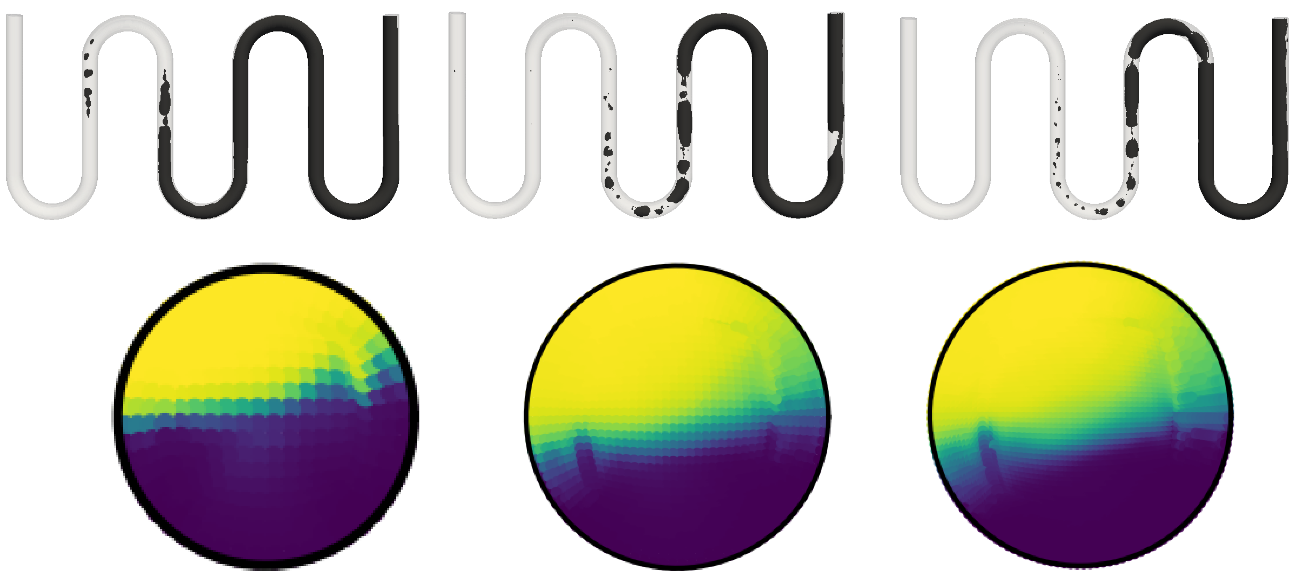
A first way to assess mesh convergence was to look at the position of the large interfaces within the computational domain: for this purpose, the instantaneous visualization of the isocontour is represented in Figure 5, for each resolution. In this flow, the phase change imposed by the parietal thermal input implied the appearance of a succession of flow regimes, ranging from dispersed bubbles to stratified wavy; however, after some time, a statistically stationary state was established, and the differences observed between two time steps only concerned slight variations in the position of the bubbles in the computational domain, while the transition positions between regimes remained constant: thus, the visualizations shown in Figure 5 were extracted when the statistically established regime was reached for these cases. It can be seen that, between a resolution of 20 and a resolution of 40 meshes per diameter, the transition between regimes did not occur at the same position in the tube: the first bubbles appeared in the middle of the second straight section in the first case, and at the beginning of the third straight section in the other; furthermore, it was not possible to distinguish between churning and slugging regimes in the lowest resolution, as was the case for the one with 40 mesh per diameter. Finally, the difference between 40 and 60 resolution did not seem significant in this visualization.
Another way of evaluating mesh convergence is to look at the averaged fields in a given section, once a statistically established flow has been reached: thus, the bottom part of Figure 5, represents the evolution of the average void fraction in section SH3, located in the last bend before the outlet (see Figure 6). Again, we saw significant differences between the 20 and 40 resolutions: indeed, the height of the free surface was much higher for the low-resolution simulation. As before, the simulations for resolutions of 40 and 60 did not seem to show significant differences.
Considering these two indicators, the results obtained with the 20 meshes per diameter resolution did not seem converged. The results obtained with resolutions at 60 and 40 meshes per diameter seemed very close. Knowing that the cost of calculating a simulation with a resolution of 60 was times higher than the same calculation with a resolution of 40, the latter appeared to be the best compromise between sufficient accuracy and a reasonable calculation cost: therefore, it was this resolution that was used in the rest of this paper.
3.2. Validation against Yang’s Case a
In this section, our modeling approach was validated against case a of Yang’s study (see Table 2).
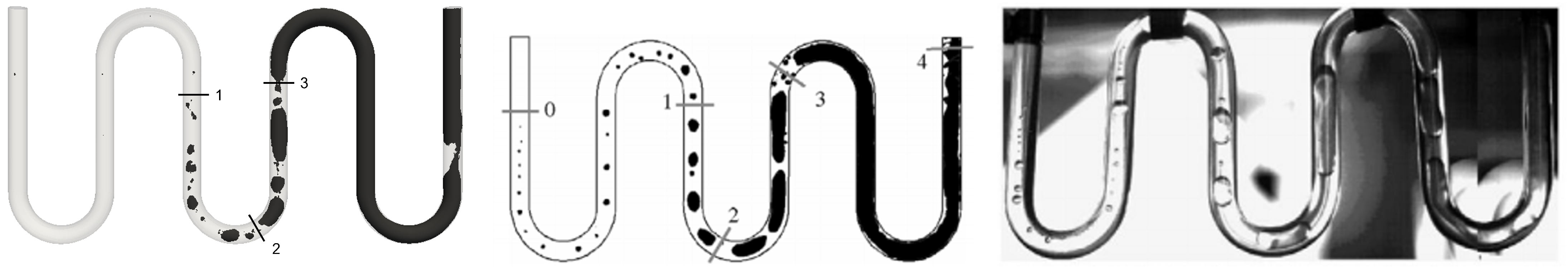
Regime transitions were the first feature of the flow that we wanted our modeling approach to be able to reproduce. Figure 7 compares the instantaneous isocontour of with the visualization proposed by Yang.
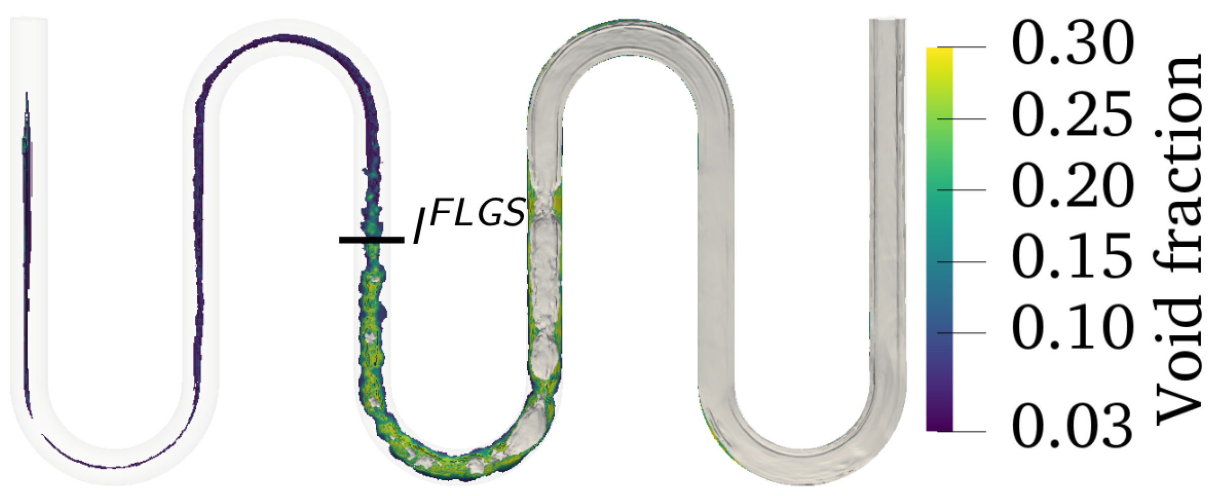
In this figure, one can observe that our approach was in satisfactory accordance with the results presented by [1]; however, in our simulations, the first bubbles appeared at the beginning of the third straight tube, whereas in the Yang simulation and experience, the first bubbles appeared right after the inlet. This difference could be explained by several factors. Firstly, our visualization only represented the isocontour , which produced the large interfaces in our modeling approach. In other words, the subgrid gas content was not represented in Figure 7: to make it appear, a second visualization of the flow regime was proposed, as shown in Figure 8, where the subgrid gas content has been added, using a color scale. In this figure, one can observe that the dispersed gas phase was created close to the inlet, due to the wall heat flux. Another reason that might explain the discrepancies was directly linked to the specification of the wall boundary condition itself. In our simulations, free convection with the ambient was considered: to do so, a convective heat transfer of was estimated, by means of the correlation of Churchill and Chu [33]. This value was consistent with the wall-ambient temperature differences involved in this calculation case; furthermore, the author did not specify the ambient temperature in the experiment room. Finally, an experimental issue, involving the injection of air bubbles at the inlet, was also possible.
Finally, we observe that the methodology employed here enabled the the positions of the regime transitions to be reproduced properly; however, with our approach, the apparition of the First Large Gas Structure (FLGS) was observed further downstream, compared to the Yang experimental and numerical results: the position of this apparition is further analyzed in the next section.
3.3. Further Analysis of the Flow Pattern
3.3.1. Apparition of the First Large Gas Structure
We assumed that the FLGS appeared in the domain when the average liquid temperature had reached the saturation temperature, meaning that, at any liquid-vapor interface, the rate of condensation was negligible, compared to the rate of evaporation. To estimate the consistency of this assumption, we used a simple 1D model, to estimate the distance from the inlet at which the liquid temperature reached the saturation temperature. If we neglected thermal losses, and assumed the fluid temperature to be homogeneous in a cross-section, then Equation (17) represented the thermal balance of the tube between the inlet and the position where :
We assumed that this distance corresponded to the apparition of the FLGS; thus, we could write:
The obtained distance was systematically compared with the one observed in the simulation. For our reference case, the distance extracted from the simulations was highlighted in Figure 8. Data, corresponding to all the cases performed in this paper, were gathered in Table 3. For all the simulations, the extracted distance was in excellent agreement with the simple model, as the maximum discrepancy was . One can also observe that this position was almost constant for all of Yang’s simulation: this point remains inexplicable to us.
3.3.2. Analysis of Average and RMS Fields
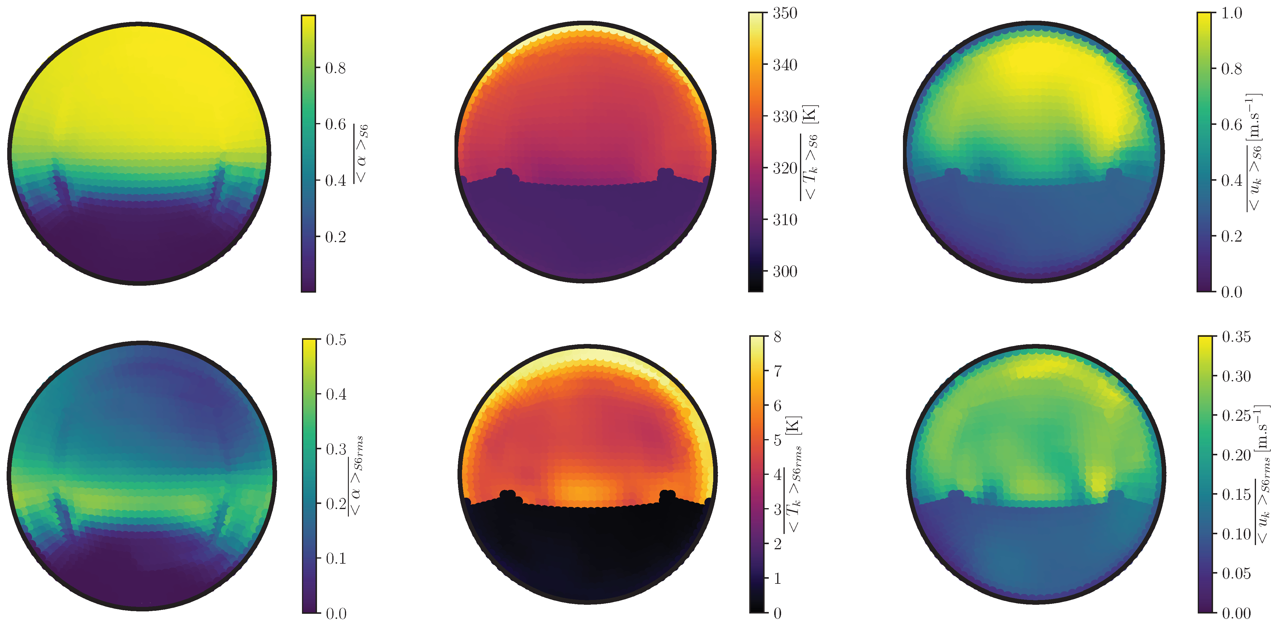
In order to further disentangle the flow in this configuration, the averaged and root mean squared (RMS) fields in section S6 were analyzed for the void fraction, the temperature and the streamwise velocity.
Void Fraction
The mean and RMS fields of the void fraction in section S6 are represented in Figure 9. For the mean field, the void fraction evolved from 0 (liquid phase) to 1 (vapor sky). On a wide band around the interface, the void fraction comprised between 0 and 1, which could be explained by a numerical diffusion of the interface, mesh influence and also the effect of passing waves; furthermore, above the interface and on both sides of the tube, the void fraction evolved from to , which was due to the presence of droplets in the vapor sky. The RMS field supported the presence of droplets, as it was not strictly equal to 0 in the vapor sky; however, droplets were only passively transported in the present version of the code. Future work should take advantage of the droplet momentum transfer closure proposed by Davy et al. [34,35]. High RMS fields were located in the vicinity of the interface, which confirmed the presence of waves in the flow: the asymmetric character of these fields could be explained by the influence of the last elbow, which implied a high asymmetric flow with respect to the vertical axis.
Temperature
The average temperature field was homogeneous in the liquid phase, and was equal to the saturation temperature, which led to a null RMS field in the liquid phase. The vapor was highly overheated at the wall; indeed, the saturation temperature was equal to , and the vapor reached at the top of the vapor sky. The temperature was continuous at the liquid–vapor interface: this resulted in a strong temperature gradient in the vapor phase.
Streamwise Velocity
The flow velocity in the streamwise direction was not homogeneous in the liquid phase (see Figure 9). The boundary condition of zero speed on the wall was verified. An asymmetric distribution was observed in the vapor sky, due to centrifugal forces induced by the previous elbow. The RMS field showed that, even if the temperature of the liquid phase was homogeneous and constant at (due to phase change), the flow was turbulent. Indeed, one can see non-zero RMS in Figure 9. The turbulent intensity, defined here as /, showed maximum deviations from the average velocity of 63% within the same section. The inertial force effects of the elbow were visible at the right of the tube in the fluid phase.
3.3.3. Stratified Wavy Regime
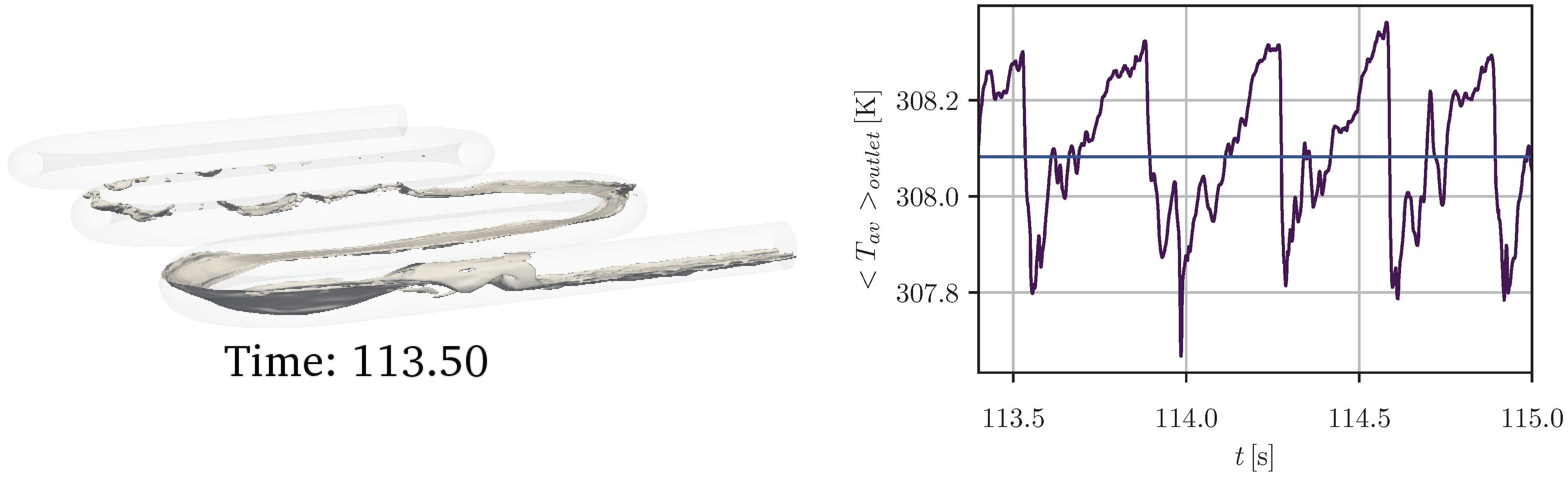
Close to the outlet, for this reference case a, a stratified wavy regime was observed in our simulation. This observation was in accordance with the regime identification made by Yang. In this regime, an interesting correlation was observed between the wave passage and the average temperature. Figure 10 shows a wave on the last straight section at the time s. The passing of a wave meant a local decrease of the void fraction, which implied a local decrease in the average temperature — as liquid temperature was lower than the vapor temperature. The time evolution of the fluid average temperature captured this phenomenon (see Figure 10-Right). The passing wave frequency was between 2 and 4 Hz. One could also see some instabilities further upstream. At this point of the study, the transition from stratified flow to stratified wavy flow was not clearly understood.
3.4. Ability of the Approach to Modeling Yang’s Different Cases
The study of Yang’s case a showed the ability of the numerical approach employed here to represent the large interfaces and transition zones between the different regimes. The study of three other cases proved the robustness of the model at adapting to various physical conditions.
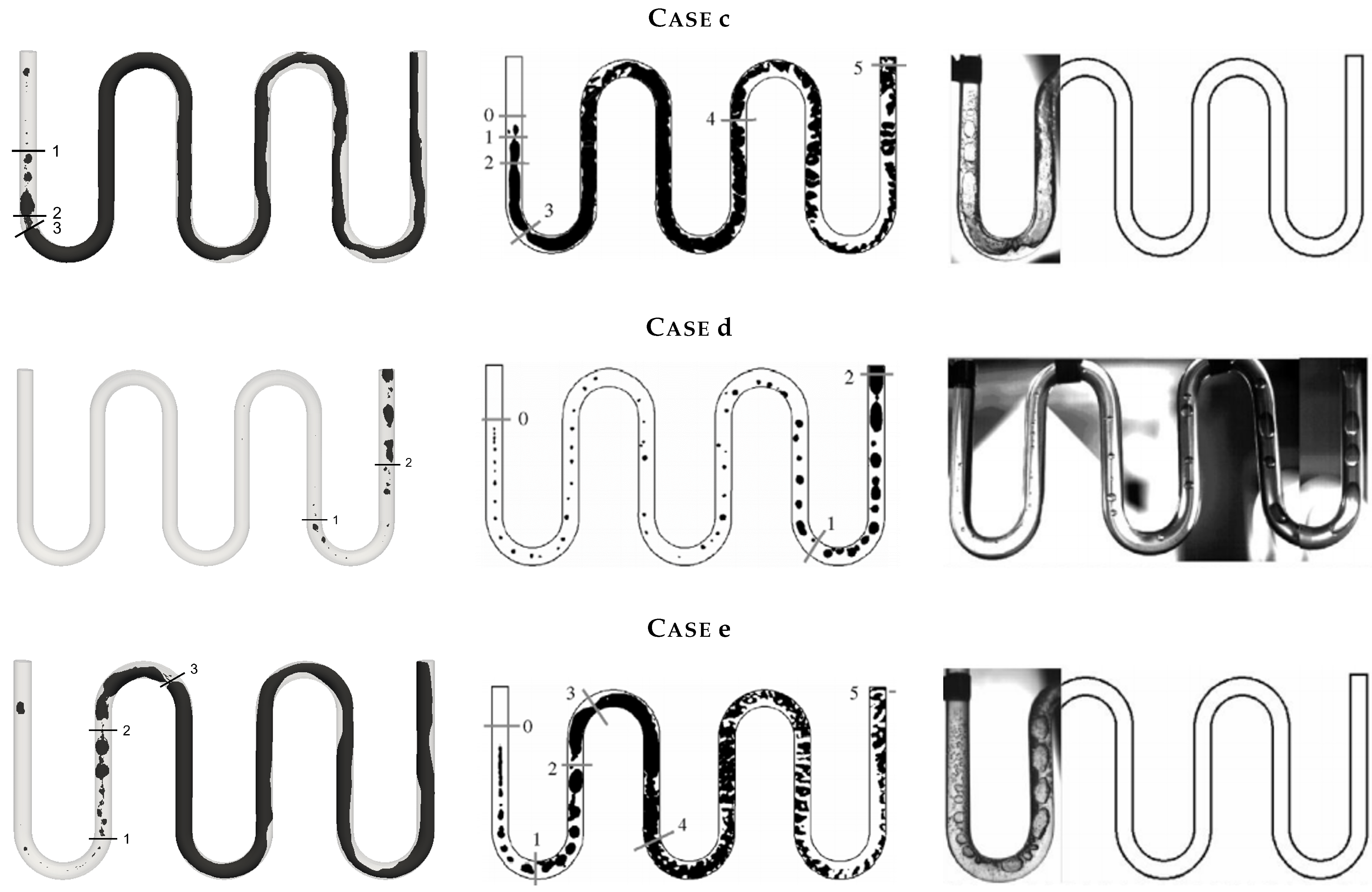
Case c, visualized on the first line of Figure 11, represented the flow for a wall heat flux of , a flow rate of and a subcooling temperature of . The vapor was created further upstream than in the reference case, because of the higher heat flow. The transition from a bubbly to a stratified regime then appeared upstream in the pipe. Differences between churn and slugs were more difficult to see; however, a stratified wavy regime seemed to occur downstream of the third elbow, which was not visible in the first case. The NEPTUNE_CFD simulations were in good agreement with the Yang simulations; however, the transition from stratified to stratified wavy flow seemed to occur further downstream in the tube in the author simulation. The photograph of the experiment had been truncated by the author for technical reasons not detailed in the article. The comparison was thus limited to the first two straight sections. In the experiment, the churn regime occurred at the entrance of the tube, which was not the case in our simulations.
Case d, visualized on the second line of Figure 11, represented the flow for a wall heat flux of , a flow rate of and a subcooling temperature of : this case was the most thermally stressed, so the bubbles should have appeared much further downstream than for the other cases. The simulations were in agreement with this predicate. The Yang simulation showed, however, a bubbly flow from the inlet to the last elbow, which was in agreement with the experiment, but seemed strange considering the control parameters. The churn and slug regimes appeared at the same location for both NEPTUNE_CFD and Fluent simulations, which differed from our experiment, for which the churn regime appeared at the fourth elbow. One should note a discontinuity at the right of the photograph: thereby, comparisons with the experiment should be tempered.
Case e, visualized on the last line of Figure 11, represented the flow for a wall heat flux of , a flow rate of and a subcooling temperature at the inlet of . This case was close to case c. The wall heat flux was lower, so the vapor should have appeared further downstream in the tube than in case c. Once again, the vapor appeared later in the NEPTUNE_CFD simulations than in the Yang simulation or our experiment. The stratified wavy flow was visualized downstream of the third elbow.
Table 3 shows that the vapor appeared at the same position in the tube for all cases in the Yang simulations, which was not consistent with the one-dimensional approach; indeed, the distance required for the fluid to reach saturation depended on the physical conditions of the case. The NEPTUNE_CFD simulations were in accordance with our simple model, as the model predicted the observed position of the FLGS, with accuracy over .
3.5. Thermal Considerations
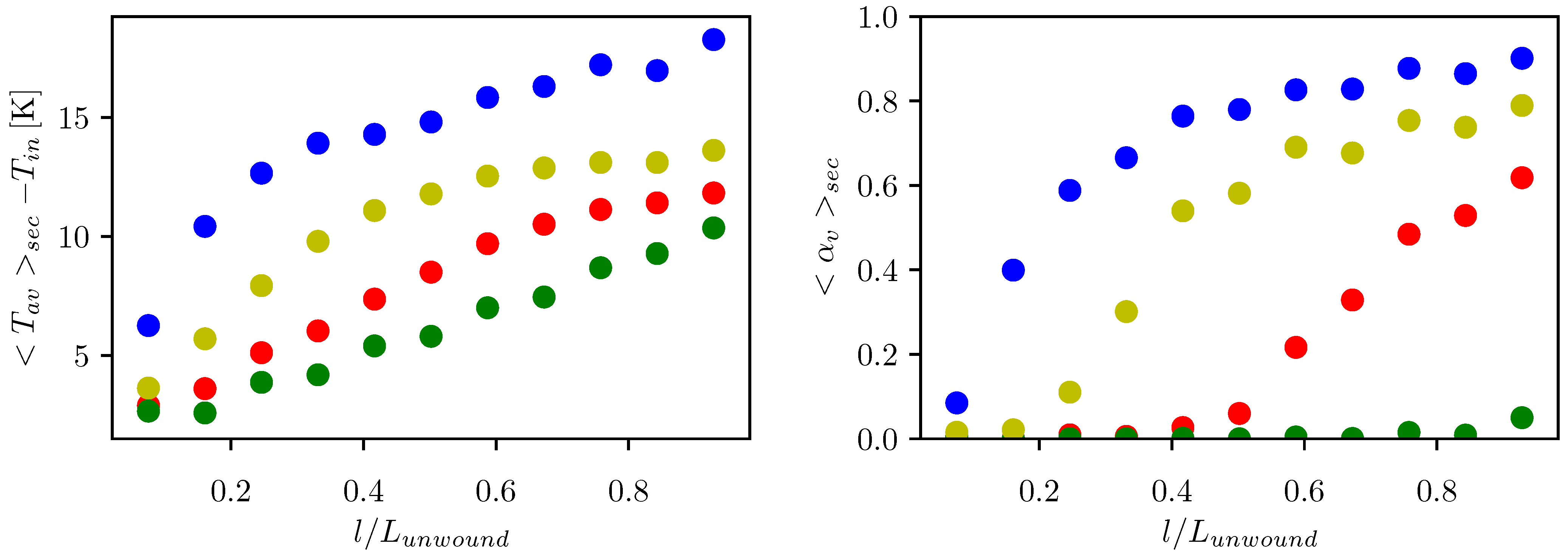
Figure 12 represents the phase-averaged fluid temperature evolution in the streamwise direction. The phase-averaged temperature (see Equation (19)) is weighted by , to consider the respective thermal inertia of the phases:
is the volume of cell i, and N is the total number of cells in the fluid domain.
Figure 12.
Averaged temperature and void fraction evolutions in the streamwise direction, for the sections defined in Figure 6, for various cases: case a in red; case c in blue; case d in green; case e in yellow. (Left): fluid average temperature. (Right): averaged void fraction.
Figure 12.
Averaged temperature and void fraction evolutions in the streamwise direction, for the sections defined in Figure 6, for various cases: case a in red; case c in blue; case d in green; case e in yellow. (Left): fluid average temperature. (Right): averaged void fraction.

In the figure, time-averaged values—calculated in all sections introduced in Figure 6—are presented. The phase-averaged temperature rise shows that for high-heat flux the rise in temperature was much faster than for a low-heat flux, where the average temperature grew slowly. The average temperature of the fluid increased along the tube as the proportion of vapor in the cross-section increased (see Figure 12). Such evolution was in accordance with a basic 1D heat balance, as proposed in Section 3.3.1; indeed, as the incident heat flux was constant and homogeneously distributed on the external surface, the amount of energy received by the fluid increased with the distance from the inlet, and thus the average temperature increased in the streamwise direction.
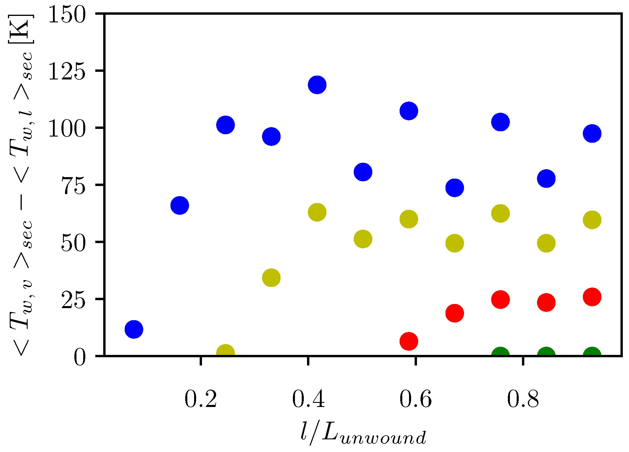
Another indicator of heat transfer in the geometry was given by the solid temperature difference, in a section transverse to the flow direction. This allowed an assessment of the temperature anisotropy in the solid, which was directly responsible for the thermomechanical stresses: the right of Figure 13 represents, for the same sections, an indicator of this wall temperature difference. Indeed, one can observe the evolution of the phase-averaged wall temperature difference . To calculate those temperatures, in each section, the wall temperature—available in any cell adjacent to the wall—was weighted by the volume fraction of the cell, as defined in Equation (20).
was the wall temperature in the fluid domain of the cell; i was the wall surface of the cell i; was the total number of meshes in contact with the wall within a cross-section.
This approach allowed the temperature of the solid to be evaluated as a function of the phase with which it was in contact. In our post-processing, the temperature difference was not represented if the vapor volume fraction was negligible in the cross-section of interest.
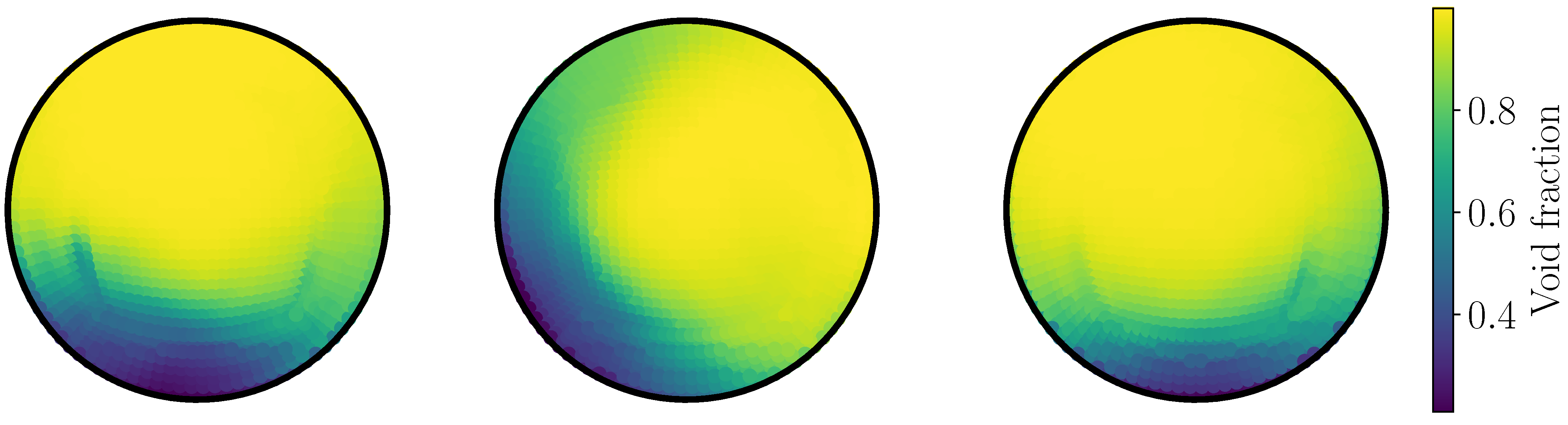
For case a, the ignition of the temperature difference appeared after of the tube, which was consistent with previous observations—see the apparition position of the FLGS in this case in Table 3. For cases c and e, it appeared around and , respectively. Finally, for case e, some discrepancies from the distance reported in Table 3 were observed; however, the positive temperature differences measured were not persistent in the domain before of the unwound length, which was consistent with the apparition position of the FLGS. The temperature difference was significantly influenced by the domain geometry—especially the bends: indeed, this phenomenon can be easily visualized by looking at the temperature evolution for case c, where temperature differences were lower in sections located in elbows of the geometry. By observing the surface wetted by the liquid in the different sections (see Figure 14, which showed the average void fraction in three successive sections), it can be seen that, on average, the wetted areas in the bends were greater than in the straight sections. Despite the fact that section B2 was located downstream of section S4, the wetted area was greater there, owing to the action of centrifugal forces present in the bends. As the convective transfer coefficient was much larger in liquid than in vapor, in sections where part of the wall was permanently in contact with the vapor, the heat flux was poorly removed from the wall in these areas, resulting in large increase in ; however, solid conduction redistributed the incident heat flux azimuthally, so that in the bends—where the wetted area was larger—a larger portion of the flux was removed by the liquid phase: this led to the decrease of the vapor wall temperature, along with the temperature difference, as shown in Figure 13. Finally, it appears here that the solid temperature difference in a cross-section of the flow was strongly correlated with the flow regime itself. Such analysis is consistent with the solid temperature field presented by [36]. This turned out to be an experimental advantage, as the measurement of the volume fraction was much more complex than that of the temperature.
The use of thermocouples placed at the top and at the bottom of the tube could thus enable identification of the flow regime inside a section of the tube.
4. Concluding Remarks
The objective of this study was to develop a numerical approach to modeling boiling flows involved in direct-steam-generation solar receivers in a Euler–Euler formalism: this formalism was selected because it allowed us to drastically limit the computational cost compared to a DNS approach, and thus to make possible the simulation of industrial or pilot scale configurations.
To this end, we identified the Yang case [1] as an excellent validation case [27]. This study presented the experimental and numerical results of boiling flow in a horizontal coil tube. The working fluid in this study was a refrigerant (R141b), which thus deviated from our initial objective; however, all the physical ingredients of the solar receiver were well present in this validation case. Moreover, the range of the control parameters explored—mass flow rate, inlet subcooling and wall heat flux—enabled the observation of a wide range of two-phase flow regimes: bubbly; churn; slugs; stratified; stratified wavy. Unfortunately, it became apparent during the course of the study that the results from this study were mainly qualitative, and therefore did not allow a quantitative evaluation of the models.
Firstly, a mesh convergence study was carried out on a reference case. This study identified that a resolution of 40 meshes per diameter enabled spatial convergence while maintaining a reasonable computational cost: this convergence was assessed on the basis of the position of the regime transitions in the computational domain, and the statistical convergence of the mean volume fraction fields. On the selected resolution, a thorough study of the flow was carried out for the reference case: this showed that our approach was able to reproduce the regime transitions identified by Yang; however, due to the nature of our approach, the bubble flow regime was simulated in a sub-mesh fashion. The study of the mean and RMS fields showed that a steady state was thermally reached in the liquid phase, which was not the case in the vapor; however, from a dynamic point of view, velocity fluctuations were observed in both phases. Moreover, the velocity of the RMS was of the same order of magnitude in both phases. Large fluctuations therefore persisted in the vapor phase, both dynamically and thermally, while only the dynamics fluctuated in the liquid phase, in a statistically established regime. A strong coupling was identified between the wall temperature and the flow regime inside the tube. Finally, the robustness of our approach was evaluated by reproducing different cases, enabling the attainment of a whole zoology of two-phase flow regimes with a satisfactory capture of the different regime transitions. The study of the average temperature and phase-averaged wall temperature differences showed, on the one hand, a very strong coupling between the flow regime and the temperature level, and, on the other hand, that the temperature gradients in a tube section can become very strong—up to 120 C—when a stratified flow regime is established. Unfortunately, no data are currently available in the literature for any quantitative evaluation of these results.
Author Contributions
Investigation, data curation, visualization, writing—original draft preparation: E.B.; software: E.B. and S.M.; conceptualization, methodology, writing—review and editing, validation, formal analysis, supervision: S.M. and A.T.; resources, project administration and funding acquisition: S.M. All authors have read and agreed to the published version of the manuscript.
Funding
This work was funded by the French “Investments for the Future” (“Investissements d’Avenir”) program managed by the National Agency for Research (ANR) under contract ANR-10-LABX-22-01 (labex SOLSTICE).
Data Availability Statement
The data presented in this study are available on reasonable request from the corresponding author.
Acknowledgments
The authors acknowledge Hélène Vernier for her preliminary work on this subject. The technical support of Nicolas Mérigoux (EDF R&D—Chatou), Hervé Neau (IMFT—Toulouse) and Maxime Pigou (IMFT—Toulouse) was greatly appreciated. Finally, the authors wish to thank Fabien Roger (SUNCNIM –Llo) for valuable discussions concerning GDV solar power plants.
Conflicts of Interest
The authors declare no conflict of interest.
Nomenclature
| Abbreviations | |
| NS | Navier–Stokes |
| CL | continuous liquid |
| CG | continuous gas |
| DG | dispersed gas |
| FLGS | First Large Gas Structure |
| RMS | Root Mean Square |
| Roman symbols | |
| u | velocity () |
| P | pressure (Pa) |
| g | gravity () |
| deformation tensor () | |
| external source tensor () | |
| I | momentum transfer () |
| H | enthalpy () |
| Q | conductive flow () |
| interfacial thermal transfer () | |
| mass-transfer-dependent enthalpy jump | |
| volumic drag force () | |
| volumic added mass force () | |
| volumic lift force () | |
| volumic turbulent dispersion force () | |
| volumic friction force () | |
| volumic viscosity penalization force () | |
| volumic surface tension force () | |
| T | temperature (K) |
| overheat temperature required for phase change (K) | |
| a | thermal diffusivity () |
| thermal capacity () | |
| Stanton number (-) | |
| D | diameter (m) |
| contact surface at the wall within a cross-section () | |
| contact surface at the wall for a specific mesh () | |
| quantity of mesh in contact with the wall in a cross-section (-) | |
| V | volume () |
| Greek symbols | |
| void fraction (-) | |
| density () | |
| dynamic viscosity () | |
| interfacial mass transfer term () | |
| Kronecker symbol | |
| heat transfer independent of mass transfer () | |
| thermal conductivity of the solid () | |
| wall heat flux () | |
| mesh thickness (m) | |
| Subscripts | |
| spatial direction | |
| phase | |
| l | liquid |
| v | vapor |
| latent | |
| saturation | |
| c | convective |
| q | quenching |
| e | evaporation |
| s | solid |
| Superscripts | |
| w | wall |
| T | turbulent |
| temporal derivative | |
References
- Yang, Z.; Peng, X.F.; Ye, P. Numerical and experimental investigation of two phase flow during boiling in a coiled tube. Int. J. Heat Mass Transf. 2008, 51, 1003–1016. [Google Scholar] [CrossRef]
- Prosperetti, A.; Tryggvason, G. Computational Methods for Multiphase Flow; Cambridge University Press: Cambridge, UK, 2007. [Google Scholar]
- Awad, M.; Muzychka, Y. Effective property models for homogeneous two-phase flows. Exp. Therm. Fluid Sci. 2008, 33, 106–113. [Google Scholar] [CrossRef]
- Hirt, C.W.; Nichols, B.D. Volume of fluid (VOF) method for the dynamics of free boundaries. J. Comput. Phys. 1981, 39, 201–225. [Google Scholar] [CrossRef]
- Osher, S.; Sethian, J.A. Fronts propagating with curvature-dependent speed: Algorithms based on Hamilton-Jacobi formulations. J. Comput. Phys. 1988, 79, 12–49. [Google Scholar] [CrossRef]
- Unverdi, S.; Tryggvason, G. A front-tracking method for viscous, incompressible multi-fluid flows. J. Comput. Phys. 1992, 100, 25–37. [Google Scholar] [CrossRef]
- Scardovelli, R.; Zaleski, S. Direct numerical simulation of free-surface and interfacial flow. Annu. Rev. Fluid Mech. 1999, 31, 567–603. [Google Scholar] [CrossRef]
- Sethian, J.; Smereka, P. Level Set methods for fluid interfaces. Annu. Rev. Fluid Mech. 2003, 35, 341–372. [Google Scholar] [CrossRef]
- Tryggvason, G.; Bunner, B.; Esmaeeli, A.; Juric, D.; Al-Rawahi, N.; Tauber, W.; Han, J.; Nas, S.; Jan, Y.J. A front-tracking method for the computations of multiphase flow. J. Comput. Phys. 2001, 169, 708–759. [Google Scholar] [CrossRef]
- Urbano, A.; Tanguy, S.; Huber, G.; Colin, C. Direct numerical simulation of nucleate boiling in micro-layer regime. Int. J. Heat Mass Transf. 2018, 123, 1128–1137. [Google Scholar] [CrossRef]
- Du Cluzeau, A.; Bois, G.; Toutant, A.; Martinez, J.M. On bubble forces in turbulent channel flows from direct numerical simulations. J. Fluid Mech. 2020, 882, A27. [Google Scholar] [CrossRef]
- Ishii, M. Thermo-Fluid Theory of Two-Phase Flow; Eyrolles: Paris, France, 1975. [Google Scholar]
- Ishii, M.; Hibiki, T. Thermo-Fluid Dynamics of Two-Phase Flow; Springer: Berlin/Heidelberg, Germany, 2006. [Google Scholar]
- Balachandar, S.; Eaton, J.K. Turbulent dispersed multiphase flow. Annu. Rev. Fluid Mech. 2010, 42, 111–133. [Google Scholar] [CrossRef]
- Mer, S.; Praud, O.; Neau, H.; Merigoux, N.; Magnaudet, J.; Roig, V. The emptying of a bottle as a test case for assessing interfacial momentum exchange models for Euler–Euler simulations of multi-scale gas-liquid flows. Int. J. Multiph. Flow 2018, 106, 109–124. [Google Scholar] [CrossRef]
- Coste, P. A Large Interface Model for two-phase CFD. Nucl. Eng. Des. 2013, 255, 38–50. [Google Scholar] [CrossRef]
- Fleau, S. Multifield Approach and Interface Locating Method for Two-Phase Flows in Nuclear Power Plant. Ph.D. Thesis, Université Paris-EST Marne-la-Vallée, Serris, Grance, 2017. [Google Scholar]
- Frederix, E.M.; Dovizio, D.; Mathur, A.; Komen, E.M. All-regime two-phase flow modeling using a novel four-field large interface simulation approach. Int. J. Multiph. Flow 2021, 145, 103822. [Google Scholar] [CrossRef]
- De Santis, A.; Colombo, M.; Hanson, B.C.; Fairweather, M. A generalized multiphase modelling approach for multiscale flows. J. Comput. Phys. 2021, 436, 110321. [Google Scholar] [CrossRef]
- Höhne, T.; Krepper, E.; Montoya, G.; Lucas, D. CFD-simulation in a heated pipe including flow patter transitions using the GENTOP concept. Nucl. Eng. Des. 2017, 322, 165–176. [Google Scholar] [CrossRef]
- Krepper, E.; Rzehak, R.; Lifante, C.; Frank, T. CFD for subcooled flow boiling: Coupling wall boiling and population balance models. Nucl. Eng. Des. 2013, 255, 330–346. [Google Scholar] [CrossRef]
- Promtong, M.; Cheung, S.C.; Yeoh, G.H.; Vahaji, S.; Tu, J. CFD study of subcooled boiling flow at elevated pressure using a mechanistic wall heat partitioning. Int. J. Mech. Mechatron. Eng. 2017, 11, 687–697. [Google Scholar]
- Eck, M.; Zarza, E.; Eickhoff, M.; Rheinländer, J.; Valenzuela, L. Applied research concerning the direct steam generation in parabolic troughs. Sol. Energy 2003, 74, 341–351. [Google Scholar] [CrossRef]
- Lobon, D.; Baglietto, E.; Valenzuela, L.; Zarza, E. Modeling direct steam generation in solar collectors with multiphase CFD. Appl. Energy 2014, 113, 1338–1348. [Google Scholar] [CrossRef]
- Kocamustafaogullari, G.; Wang, Z. An experimental study on local interfacial. Int. J. Multiph. Flow 1991, 17, 553–572. [Google Scholar] [CrossRef]
- Dinsenmeyer, R. Etude des Écoulements avec Changement de Phase: Application à L’évaporation Directe dans les Centrales Solaires à Concentration. Ph.D. Thesis, Université Grenoble Alpes, Saint-Martin-d’Hères France, 2015. [Google Scholar]
- Dinsenmeyer, R.; Fourmigué, J.F.; Caney, N.; Marty, P. Volume of fluid approach of boiling flows in concentrated solar plants. Int. J. Heat Fluid Flow 2017, 65, 177–191. [Google Scholar] [CrossRef]
- Patankar, S.V.; Spalding, D.B. A calculation procedure for heat, mass and momentum transfer in three-dimensional parabolic flows. Int. J. Heat Mass Transf. 1972, 15, 1787–1806. [Google Scholar] [CrossRef]
- Mimouni, S.; Boucker, M.; Laviéville, J.; Guelfi, A.; Bestion, D. Modelling and computation of cavitation and boiling bubbly flows with the NEPTUNE-CFD code. Nucl. Eng. Des. 2008, 238, 680–692. [Google Scholar] [CrossRef]
- Hsu, Y. On the size range of active nucleation cavities on a heating surface. J. Heat Transf. 1962, 84, 207–213. [Google Scholar] [CrossRef]
- Kurul, N.; Podowski, M. Multidimensional Effects in Forced Convection Subcooled Boiling. In Proceedings of the International Heat Transfer Conference, Jerusalem, Israel, 19–24 August 1990. [Google Scholar]
- Unal, H. Maximum bubble diameter, maximum bubble growth time and bubble growth rate during subcooled nucleate flow boiling of water up to 17.7 MN/m2. Int. J. Heat Mass Transf. 1976, 19, 643–649. [Google Scholar] [CrossRef]
- Churchill, S.W.; Chu, H.H. Correlating equations for laminar and turbulent free convection from a horizontal cylinder. Int. J. Heat Mass Transf. 1975, 18, 1049–1053. [Google Scholar] [CrossRef]
- Davy, G.; Reyssat, E.; Mimouni, S. CFD modeling of two-phase flows in cracks. In Proceedings of the 8th Workshop on Computational Fluid Dynamics for Nuclear Reactor Safety—CFD4NRS-8, Paris, France, 25–27 November 2020. [Google Scholar]
- Davy, G.; Reyssat, E.; Vincent, S.; Mimouni, S. Euler–Euler simulations of condensing two-phase flows in mini-channel: Combination of sub-grid approach and an interface capturing approach. Int. J. Multiph. Flow 2022, 149, 103964. [Google Scholar] [CrossRef]
- Pal, R.K.; K., R.K. Thermo-hydrodynamic modeling of flow boiling through the horizontal tube using Eulerian two-fluid modeling approach. Int. J. Heat Mass Transf. 2021, 168, 120794. [Google Scholar] [CrossRef]
Figure 1.
Schematic of interfacial closure terms—adapted from [15]. In our approach, the continuous and dispersed gas belonged to the same numerical field.
Figure 1.
Schematic of interfacial closure terms—adapted from [15]. In our approach, the continuous and dispersed gas belonged to the same numerical field.

Figure 2.
Schematic of Yang’s experiment tube [1].
Figure 2.
Schematic of Yang’s experiment tube [1].

Figure 3.
Parietal heat flux distribution diagram [26].
Figure 3.
Parietal heat flux distribution diagram [26].

Figure 4.
Representation of the mesh. (Left): highlight of the coupling surface. (Right): cross-sectional view of fluid and solid meshes.
Figure 4.
Representation of the mesh. (Left): highlight of the coupling surface. (Right): cross-sectional view of fluid and solid meshes.

Figure 5.
Mesh convergence analysis: (left); (center); (right). (Top): regime identification—instantaneous visualization of isocontour produced the large interfaces in the domain. (Bottom): average fields of void fraction in section SH3.
Figure 5.
Mesh convergence analysis: (left); (center); (right). (Top): regime identification—instantaneous visualization of isocontour produced the large interfaces in the domain. (Bottom): average fields of void fraction in section SH3.

Figure 6.
Schematic of the different sections of interest.

Figure 7.
Comparison of the obtained regime transition to Yang’s results [1]. (Left): NEPTUNE_CFD simulation—instantaneous visualization of isocontour . (Center): Fluent simulations [1]. (Right): Experience [1]. Flow regimes 0–1: bubbly, 1–2: churn, 2–3: slug, 3–4: stratified.

Figure 8.
Instantaneous visualization of the vapor content in the calculation domain. Large interfaces were produced by the isocontour in gray, and the dispersed bubbles are represented by the color map. The apparition of the First Large Gas Structure is highlighted.
Figure 8.
Instantaneous visualization of the vapor content in the calculation domain. Large interfaces were produced by the isocontour in gray, and the dispersed bubbles are represented by the color map. The apparition of the First Large Gas Structure is highlighted.

Figure 9.
Average and RMS fields in section S6: void fraction, temperature and streamwise velocity. The top line shows the average fields, while the bottom one presents the associated RMS.
Figure 9.
Average and RMS fields in section S6: void fraction, temperature and streamwise velocity. The top line shows the average fields, while the bottom one presents the associated RMS.

Figure 10.
Visualization of the stratified wavy regime. (Left): instantaneous visualization of isocontour . (Right): time evolution of the phase-averaged mean temperature at the outlet: purple—instantaneous value; blue—time-averaged value.
Figure 10.
Visualization of the stratified wavy regime. (Left): instantaneous visualization of isocontour . (Right): time evolution of the phase-averaged mean temperature at the outlet: purple—instantaneous value; blue—time-averaged value.

Figure 11.
Comparison of the obtained regime transition with the results of Yang [1]. (Left): NEPTUNE_CFD simulation—instantaneous visualization of isocontour . (Center): Fluent simulations [1]. (Right): Experiment [1]. Each line corresponds to a different case (see Table 2 for the values of the different control parameters). Flow regimes 0–1: bubbly, 1–2: churn, 2–3: slug, 3–4: stratified, 4–5: wavy.

Figure 13.
Evolution of the phase-averaged wall temperature difference in the streamwise direction for various cases: case a in red; case c in blue; case d in green; case e in yellow.
Figure 13.
Evolution of the phase-averaged wall temperature difference in the streamwise direction for various cases: case a in red; case c in blue; case d in green; case e in yellow.

Figure 14.
Average fields of void fraction in case c: section 4 (left); section B2 (center); section 5 (right).
Figure 14.
Average fields of void fraction in case c: section 4 (left); section B2 (center); section 5 (right).


Table 1.
Physical properties of quartz at 20 C.
| [W m K] | [kg m] | [J kg K] |
|---|---|---|
| 1.4 | 2650 | 700 |
Table 2.
Available experimental configurations.
| Case | [W m] | Q [L h] | Subcooling [K] |
|---|---|---|---|
| a | 6888 | 10 | 8.5 |
| b | 17,848 | 10 | 8.5 |
| c | 24,874 | 10 | 8.5 |
| d | 6888 | 15 | 10.5 |
| e | 17,848 | 15 | 8.5 |
| f | 24,874 | 15 | 8.5 |
Table 3.
Apparition position of the First Large Gas Structure for all the simulated cases.
| Case | Model | ||
|---|---|---|---|
| 1D heat balance (Equation (18)) | 0.45 | ||
| a | NEPTUNE_CFD | 0.42 | 3 |
| FLUENT YANG | 0.08 | 37 | |
| 1D heat balance (Equation (18)) | 0.12 | ||
| c | NEPTUNE_CFD | 0.08 | 4 |
| FLUENT YANG | 0.06 | 6 | |
| 1D heat balance (Equation (18)) | 0.84 | ||
| d | NEPTUNE_CFD | 0.91 | 7 |
| FLUENT YANG | 0.06 | 78 | |
| 1D heat balance (Equation (18)) | 0.26 | ||
| e | NEPTUNE_CFD | 0.20 | 6 |
| FLUENT YANG | 0.06 | 20 |
Disclaimer/Publisher’s Note: The statements, opinions and data contained in all publications are solely those of the individual author(s) and contributor(s) and not of MDPI and/or the editor(s). MDPI and/or the editor(s) disclaim responsibility for any injury to people or property resulting from any ideas, methods, instructions or products referred to in the content. |
© 2023 by the authors. Licensee MDPI, Basel, Switzerland. This article is an open access article distributed under the terms and conditions of the Creative Commons Attribution (CC BY) license (https://creativecommons.org/licenses/by/4.0/).
Share and Cite
MDPI and ACS Style
Butaye, E.; Toutant, A.; Mer, S. Euler–Euler Multi-Scale Simulations of Internal Boiling Flow with Conjugated Heat Transfer. Appl. Mech. 2023, 4, 191-209. https://doi.org/10.3390/applmech4010011
AMA Style
Butaye E, Toutant A, Mer S. Euler–Euler Multi-Scale Simulations of Internal Boiling Flow with Conjugated Heat Transfer. Applied Mechanics. 2023; 4(1):191-209. https://doi.org/10.3390/applmech4010011
Chicago/Turabian StyleButaye, Edouard, Adrien Toutant, and Samuel Mer. 2023. "Euler–Euler Multi-Scale Simulations of Internal Boiling Flow with Conjugated Heat Transfer" Applied Mechanics 4, no. 1: 191-209. https://doi.org/10.3390/applmech4010011