Article

Understanding Raman Spectral Based Classifications with Convolutional Neural Networks Using Practical Examples of Fungal Spores and Carotenoid-Pigmented Microorganisms

1
Faculty of Life Sciences, Rhine-Waal University of Applied Sciences, Marie-Curie-Straße 1, 47533 Kleve, Germany
2
Department of Robotics, Perception, and Learning, KTH Royal Institute of Technology, 10044 Stockholm, Sweden
3
Institute for Bioengineering, University of Edinburgh, Edinburgh EH9 3DW , UK
*
Author to whom correspondence should be addressed.
AI 2023, 4(1), 114-127; https://doi.org/10.3390/ai4010006
Submission received: 15 November 2022 / Revised: 9 January 2023 / Accepted: 11 January 2023 / Published: 18 January 2023

Abstract

:
Numerous publications showing that robust prediction models for microorganisms based on Raman micro-spectroscopy in combination with chemometric methods are feasible, often with very precise predictions. Advances in machine learning and easier accessibility to software make it increasingly easy for users to generate predictive models from complex data. However, the question regarding why those predictions are so accurate receives much less attention. In our work, we use Raman spectroscopic data of fungal spores and carotenoid-containing microorganisms to show that it is often not the position of the peaks or the subtle differences in the band ratios of the spectra, due to small differences in the chemical composition of the organisms, that allow accurate classification. Rather, it can be characteristic effects on the baselines of Raman spectra in biochemically similar microorganisms that can be enhanced by certain data pretreatment methods or even neutral-looking spectral regions can be of great importance for a convolutional neural network. Using a method called Gradient-weighted Class Activation Mapping, we attempt to peer into the black box of convolutional neural networks in microbiological applications and show which Raman spectral regions are responsible for accurate classification.

1. Introduction

Rapid and accurate identification of microorganisms is important for a variety of reasons. For example, in medical diagnostics for rapid and correct treatment of patients and in food processing to ensure safe products. Many methods for differentiating microorganisms are based on their cultivation. This is always associated with a high expenditure of time and materials. There are faster options such as DNA-based methods or matrix-assisted laser desorption ionization-time of flight mass spectroscopy (MALDI-TOF MS). Methods based on optical molecular spectroscopy such as Raman spectroscopy can also be used to differentiate microorganisms [1]. For this, it is necessary to create a reference data set of appropriate Raman spectra and then train models to be able to make predictions for new unknown spectra. Numerous studies have shown that robust prediction models for microorganisms based on Raman micro-spectroscopy in combination with chemometric methods are not only feasible, but often very accurate [1,2,3,4]. Even single cells of bacteria can be differentiated using surface-enhanced Raman microscopy or specific metal substrates [5,6,7], which could make time-consuming pre-enrichment and cultivation unnecessary. In our own studies, we used Raman microscopy to develop predictive models to identify different isolates and species of fungal spores [8] and to differentiate between 21 species of bacteria and yeasts [9]. Here, we were able to get very accurate predictions with accuracies of over 98% using support vector machines (SVM). Advances in machine learning and publicly available software make it increasingly easy for users to generate reliable predictive models from complex data.
When these methods are used outside of the core machine learning research field, one aspect is not discussed as often, and that is the question of why these models allow such accurate predictions. A publication that partially addresses this question by Kanno et al. uses random forest machine learning to highlight the top features of a Raman spectral-based predictive model for differentiating microorganisms [10]. Small differences in the biochemical composition of the microorganisms lead to different Raman spectra, which makes the differentiation possible [1,11] with the right amount and quality of data. There can be various influences on a Raman spectrum, most of which can be eliminated by standardizing the measurement and environmental parameters. Influencing factors on Raman spectra of microorganisms, such as the culture medium used [12,13] or the incubation time [14] can be easily standardized. Despite standardization of many parameters, mathematical pre-treatment of the data is in many cases not only recommendable but crucial for effective prediction models [15]. Influences on the baseline, for example caused by interfering fluorescence, or differences in the overall intensity of a Raman spectrum, can be eliminated by baseline correction and normalization. Smoothing algorithms may also be able to prevent nonspecific noise from being misinterpreted as a feature. Predictive models can also be optimized by reducing dimensions of data via principal component analysis (PCA), and the associated elimination of features that are unnecessary or disturbing for accurate predictions [16].
In this work, we investigate whether it is really small differences in the bands of the Raman spectra that allow differentiation or whether completely different effects play a role. To address this question, we trained convolutional neural network (CNN) models with two data sets from previous publications [8,9]. One of the datasets contains the Raman spectra of fungal spores, which partly shows an extremely high similarity between some fungal isolates and species, and the other dataset [9] contains certain microorganisms with carotenoid pigments, which are considered to be a particularly good distinguishing feature [17].
While neural network-based methods have successfully propelled the fields of artificial intelligence (AI) to new heights, the interpretability and exploitability of such methods are still an active research area [18,19]. One of the most established methods for visual explanation of classification results using CNN is Gradient-weighted Class Activation Mapping (Grad-CAM) [20,21]. Grad-CAM is able to identify important neurons of the model given the classification task. This can be used to visually explain “where” the network places its attention when making a prediction. Grad-CAM is applicable to a wide range of convolutional network models; in this work, we use it to highlight the Raman spectra parts that are most crucial for prediction by considering the spectra as a 1D image.

2. Materials and Methods

2.1. Fungal Spores and Carotenoid-Containing Microorganisms

Parameters for cultivation and isolation of fungal spores can be taken from the 2021 publication by Hetjens et al. [8]. The details of cultivation of the microorganisms can be taken from the March 2022 publication by Tewes et al. [9]. The names and abbreviations of each used species are depicted in Table 1, as well as the number of Raman spectra.

2.2. Sample Preparation

The conidia and bacterial suspensions were placed on a SiO2-protected silver mirror slide (PFR14-P02, Thorlabs, Lübeck, Germany) under sterile conditions. The silver slide was placed on the motorized stage of the Raman system. Areas with spores or carotenoid-containing microorganisms were localized using the microscope (100×). Before analyzing new samples, the slide was cleaned with acetone using a cotton pad, afterwards with ethanol and a virgin fibre tissue wiper, and rinsed with sterile deionized water. The detailed description of sample preparation can be found in publications [8] (fungal spores) and [9] (carotenoid-containing microorganisms).

2.3. Spectral Recording

For all measurements a confocal Raman microscope (inVia Renishaw, Gloucestershire, UK) with an excitation wavelength of 633 nm and a 100× lens (numerical aperture of 0.85) was used. The conidia spores were measured using 1.5 s exposure time at about 0.7 mW on sample (laser diameter about 5 µm) and 15 accumulations per spectrum. All carotenoid-containing microorganisms were analyzed with an exposure time of 1.5 s at about 3.5 mW laser power on sample (laser diameter about 7.5 µm). The spectral resolution is about 1.1 wavenumbers. The detailed description of the spectral recording parameters can be found in publications [8] (fungal spores) and [9] (carotenoid-containing microorganisms).

2.4. Data Preprocessing and Model Development
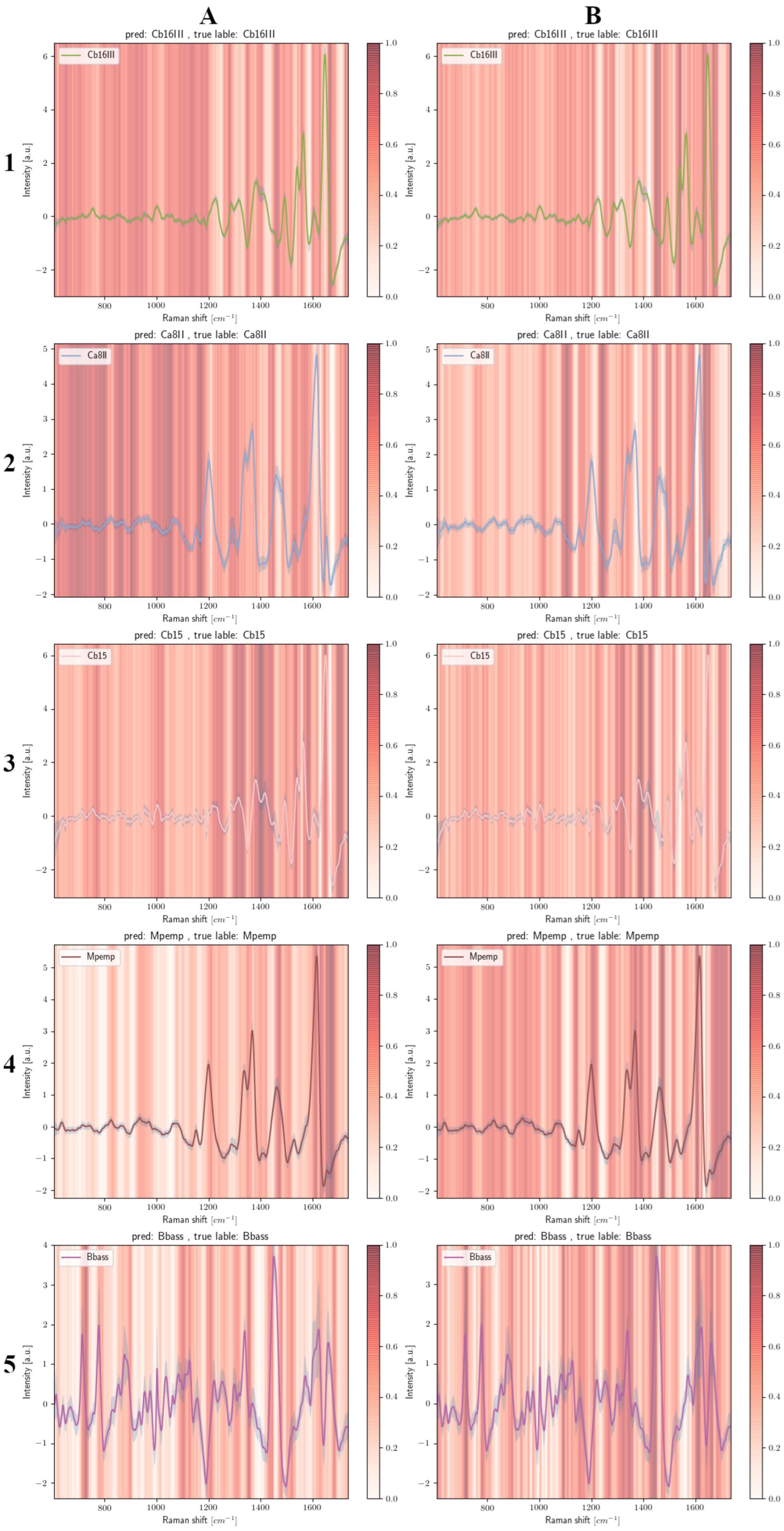
For data preprocessing, MATLAB R2021b was used (MathWorks, Natick, MA, USA). After the spectra were interpolated, baseline correction and smoothing using a low pass filter (LPF) was carried out. The appropriate LPF code for this can be found in the Supplementary Material of [22]. All spectra were normalized (z-score). To visualize first data patterns and to allow a rough estimation on the classifiability, a PCA was performed. However, for a later application of the neural networks, the complete pre-treated spectra were used and not principal components (PCs). Two independent models with the same architecture were created for fungal spores and for the carotenoid-pigmented microorganisms. For both types of data (spores and carotenoid-containing microorganisms), two models each were trained with the same settings but different weight initialization to localize possible random changes in the areas important to the model (later determined by Grad-CAM).
The models, trained using TensorFlow version 2.6.2, consist of three convolutional layers with 16 filters and a kernel size of five for each layer. The convolutional layers are followed by batch normalization, rectified linear unit (ReLU) activation layers, and a max pooling layer. After a global average pooling operation, a fully connected layer with 256 neurons, ReLU activations and dropout of 0.3 is added before at the output layer of dimension 5 using a softmax activation. In total the model consists of 8421 trainable parameters. We employ the commonly used Adam optimizers with a learning rate of 0.0001 and use the Sparse Categorical Cross-Entropy loss. The model is trained for 1500 epochs using a batch size of 64.

2.5. Grad-CAM

We use Grad-CAM in order to retrieve the activation given an input data and correct prediction. As Grad-CAM returns the pooled gradients up to the last convolutional layer, a heatmap of the size 256 was obtained and resized to the input data using OpenCV [23] resize function with a bilinear interpolation. Each class-specific sample is aggregated in order to obtain the mean activation maps of a class, if the prediction of it was correct.

3. Results and Discussion

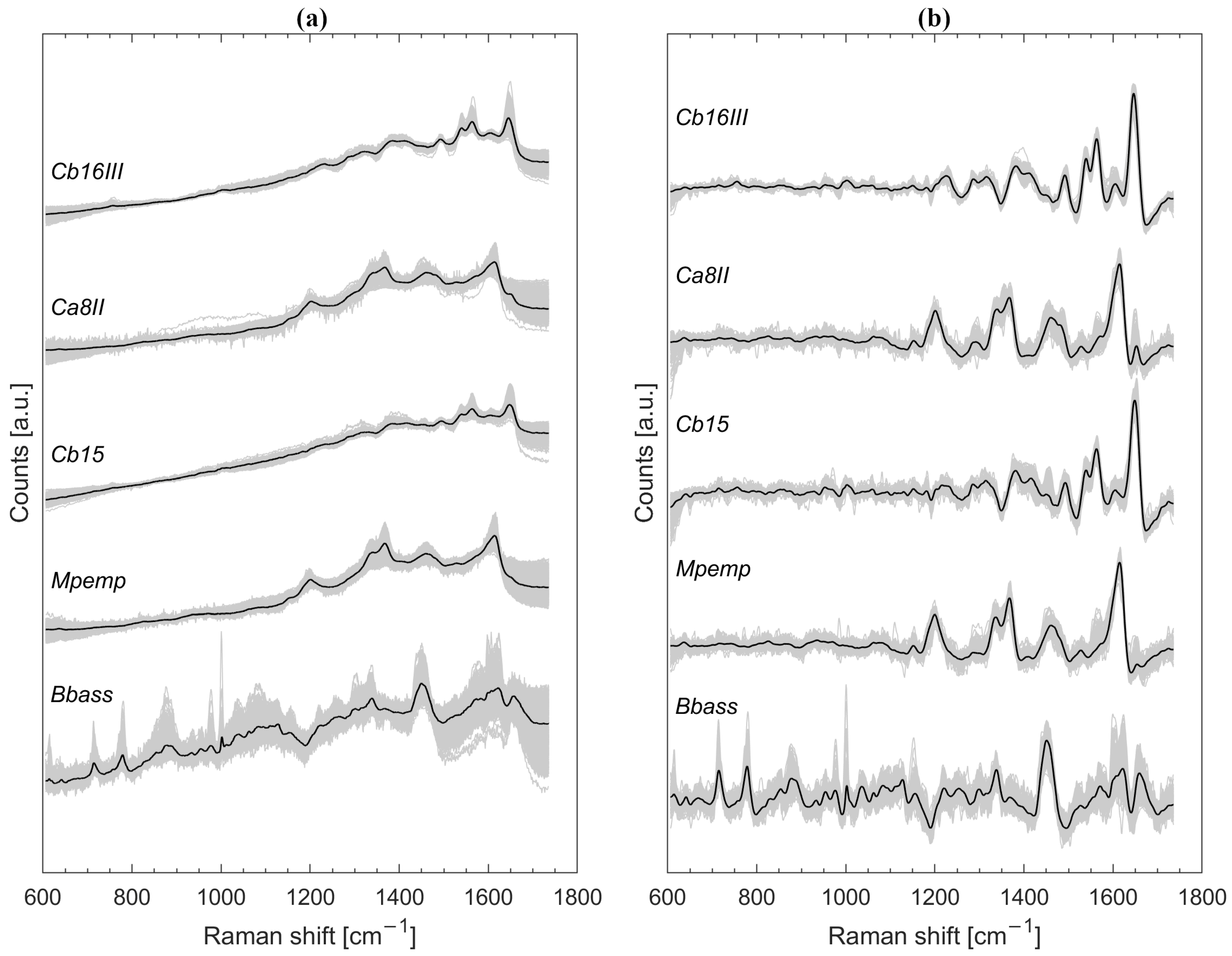
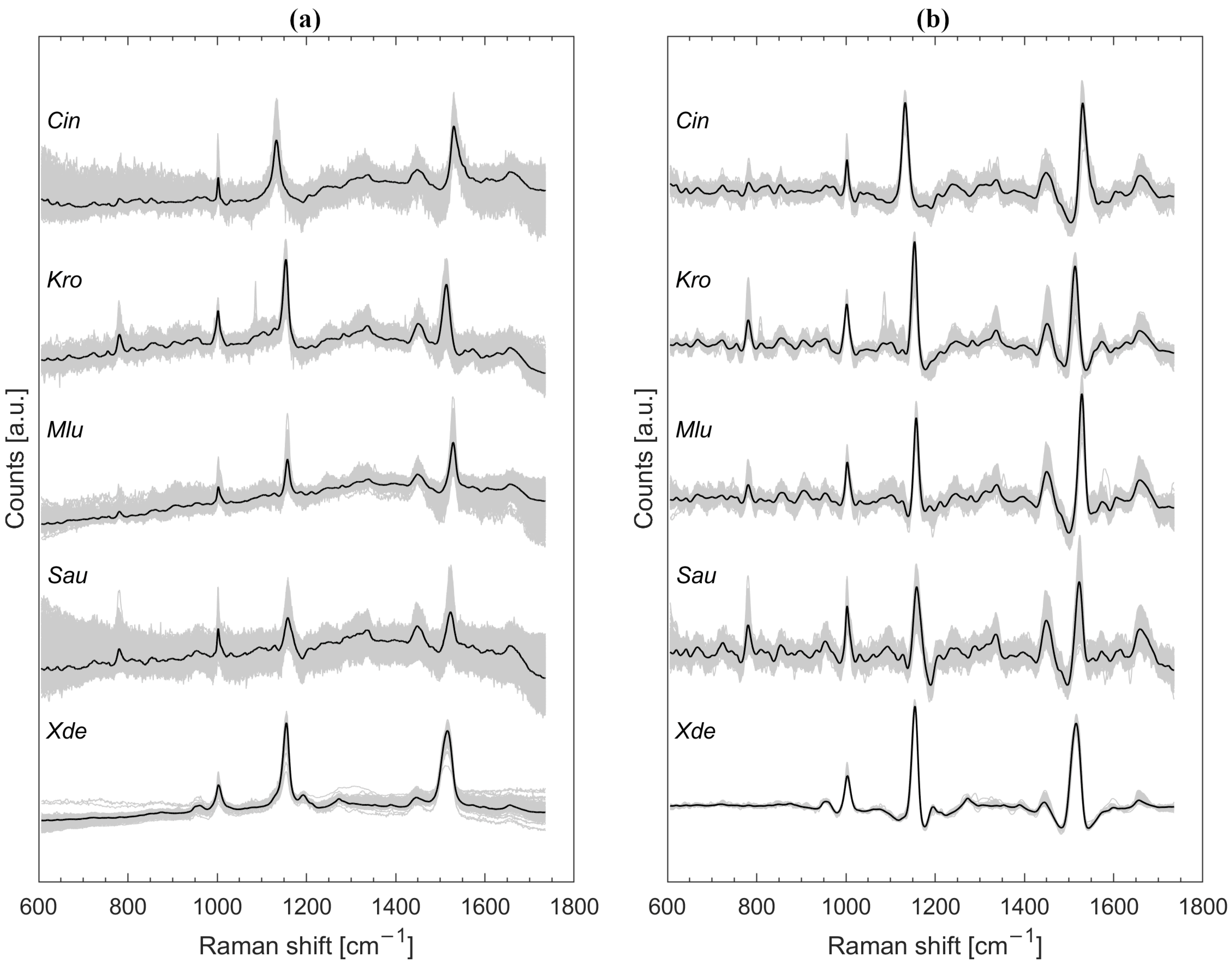
3.1. Raman Spectra Untreated and Preprocessed

Due to diverse influences on Raman spectra that are not based on the bio-chemical differences of individual species, some data pretreatment is of great importance for the classification of different microorganisms [24,25]. For this reason, models with untreated data were not generated and examined in this work.
Figure 1 shows the spectra of the fungal spores. Particularly high similarities can be seen between Cb16III and Cb15 and between Ca8II and Mpemp. The greatest internal variation of the spectra is present at Bbass, where interfering fluorescence was most prevalent. Noticeable are the effects at the beginning and at the end of the pretreated Raman spectra (Figure 1b), which are caused by the LPF used, where the spectra appear to be “pulled” downwards (approx. 600 cm−1) or show a kink (approx. 1675 cm−1).
The untreated Raman spectra of the carotenoid-containing microorganisms (Figure 2a) show the largest scatter in the range between 600 and 1000 wavenumbers; particularly well observable in Cin and Sau. After data pre-treatment, this variation is much smaller (Figure 2b). The two most pronounced peaks in all spectra from Figure 2 at about 1150 and 1525 cm−1 represent carotenoids [17]. It can be observed that these peaks shift slightly to the left or right depending on the species, which already suggests a good classifiability. Slight negative slopes are also seen in the pretreated spectra (Figure 2b) before and after the strongly pronounced peak at about 1525 cm−1. Sau and Xde also show a clear drop after the second strongly pronounced peak at about 1150 cm−1.

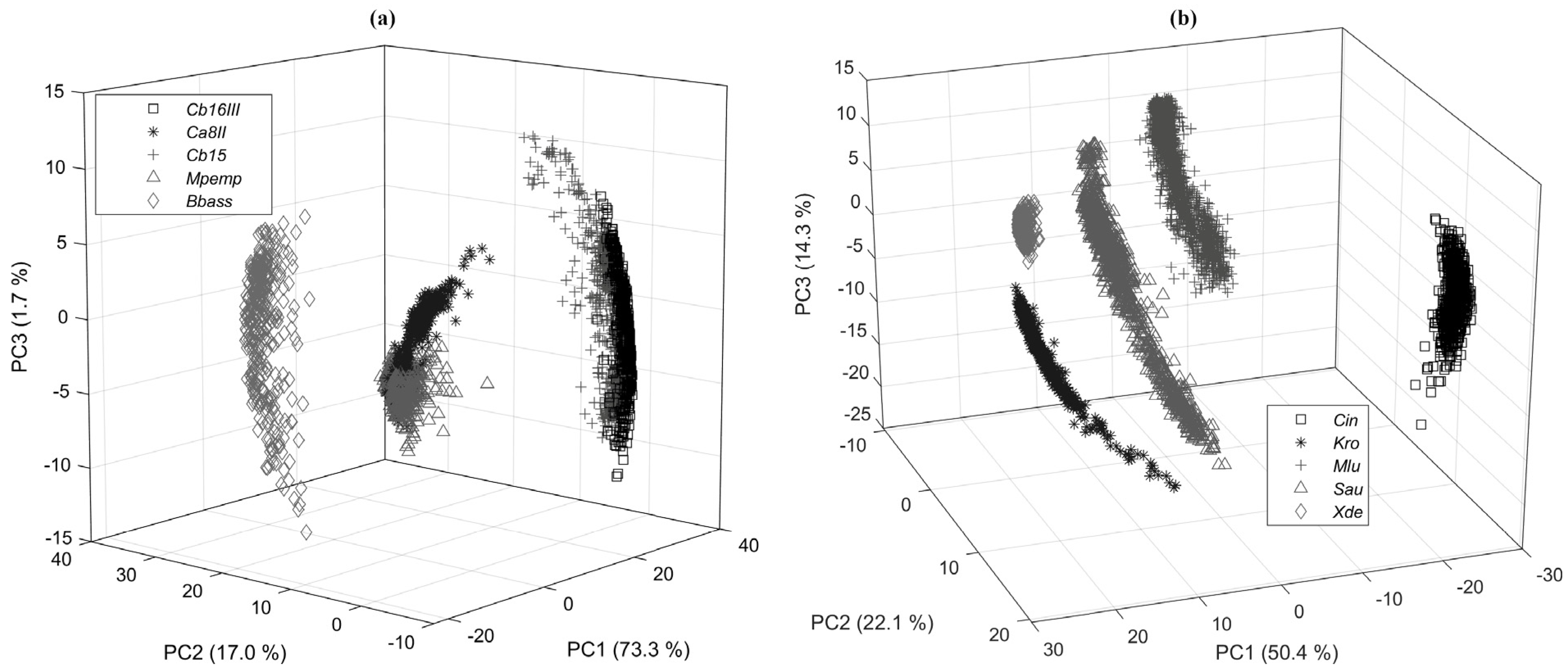
3.2. PCA for General Estimation of the Classifiability

PCs describing the most variance are not always the best variables for classification [26]. It is possible that PCs describing less variance are better for classification as PCs describing much variance. Nevertheless, PCA is a relatively simple and solid method to recognize patterns in large data sets [27].
Figure 3a shows quite clearly that the first three PCs have difficulty spatially separating Cb16III and Cb15. The clusters of Ca8II and Mpemp also merge. Bbass is the most distinct from the rest of the data and is clearly separated. As already suggested by the observation of the peaks triggered by the carotenoids in Figure 2b, the Raman spectra separate clearly from each other when the first three PCs are plotted (Figure 3b).

3.3. Predictive Models and Cross-Validation

In order to evaluate the predictive CNN models, 5-fold cross-validation was performed, resulting in a test split of 20% of the data. In order to avoid overfitting, we use 15% of the training dataset as a validation set and save the best performing model on it. This model is then evaluated on the held-out test set. The average precision, recall, F1-score and support for model 1 with fungal spores is reported in Table 2. The precision for Cb16III (0.98), Cb15 (0.96) and Bbass (1.0) is very high. Model 1 is less precise for the spores Mpemp (0.89) and Ca8II (0.88), but the correct predictions are still almost 90%. The model 2 for fungal spores with the same architecture as model 1 shows similar values for precision, recall, F1-score and support (Table 3). Large differences would be a sign of an insufficient data set; this is not the case here.
Both the performance parameters for the first model for carotenoid-containing microorganisms (Table 4) and those for the second model (Table 5) show a value of 1.0 everywhere, indicating a 100% correct identification of every species.

3.4. Grad-CAM Results

The Grad-CAM visualization results are obtained by aggregating the activation plots for each correctly predicted classification results and normalizing them between 0 and 1. The mean and variance of the specific class spectra is plotted as solid line and shaded region, respectively. The activations are plotted as vertical strips over the spectra signal. The darker a particular stripe at a certain wavelength appears, the more relevant the region is for the model to make its prediction (scale next to each plot in Figure 4 and Figure 5). Note that as the aggregation over all correctly classified spectra of a particular class is shown, we can infer what regions are generally more or less important for the model to make correct predictions, however, it does not necessarily mean that each signal triggers the attention on all highlighted areas.

3.4.1. Fungal Spores

Figure 4(A1–5,B1–5) show the mean spectrum of the respective fungal spores and the spectral areas used by the neural networks for classification. In the case of Cb16III (Figure 4(A1)), many areas in the shorter wavenumber regions (about 600–1200 cm−1) are used by the model. This spectral region has comparatively weak signals, and the somewhat more pronounced signatures at about 753 and 1001 cm−1 are even considered less important by model 1. The more distinct signatures in the range of 1200 to 1565 cm−1 are also used less and it is mainly the edges just before and after signatures that are highlighted by Grad-CAM. Thus, for Cb16III in model 1 (Figure 4(A1), the areas 1464 cm−1 and 1668 cm−1 are highly important for classification, although there are no peaks there. The regions highlighted by Grad-CAM in the second model (Figure 4(B1)) are relatively similar to model 1, but the regions in the short wavenumber range (600 to 1200 cm−1) receive somewhat less attention than in model 1. The only distinct peak of Cb16III highlighted in deep red by Grad-CAM in model 2 is the sharp partial peak at 1538 cm−1.
The marked Grad-CAM regions of model 1 of the spore isolate Cb15 (Figure 4(A3)), which is Raman spectroscopically very similar to Cb16III, looks almost complementary to Cb16III (Figure 4(A1)). The short wavenumber region receives less attention except for the signatures at about 753 and 1001 cm−1 (Figure 4(A3)). Additionally, exactly complementary, model 1 completely omits the regions before and after the most pronounced peak at about 1649 cm−1, whereas these regions are important in Cb16III. The Grad-CAM marked areas of Cb15 of model 1 (Figure 4(A3)) that are similar to Cb15 of model 2 (Figure 4(B3)), where in model 1 it is exactly the area between the double peak at 1383 and 1413 cm−1 that is marked in deep red, and in model 2, it is more the actual peaks and not the area that is in between. Noticeable in Cb15 in both model 1 and model 2 are the Grad-CAM highlights in the area after 1647 cm−1 which is mainly due to the baseline filter used (comparison to untreated spectrum of Cb15 in Figure 1a). It is likely that the effect on small differences in fluorescence on Raman spectra after data pretreatment will lead to boosted features. Of course, it must not be ignored that if other baseline subtraction methods had been used, the models would likely have used other spectral regions for classification. We have started to investigate this as well, but even baseline filters that perform better lead to models where rather supposedly unspecific regions are used for classification (Supplementary material Figure S1).
Metarhizium-species include, like the carotenoid-containing microorganisms, colored pigments. The Raman spectra of Metarhizium showed characteristic bands at about 1380–1400 cm−1 and 1580–1600 cm−1, indicating that both conidia might contain melanin [28]. Since under the consideration of the collected Raman spectroscopic data, the type of pigment of the studied Metarhizium fungal isolates does not differ, it is other variations that provide the rash for a successful classification. Comparing the untreated spectra from Figure 1a of Cb16III and Cb15, it is clear, firstly, that the spectra are extremely similar, and secondly, that the expression of the peaks is generally slightly weaker for Cb15. After data pretreatment, this effect is hardly perceptible (Figure 1b).
Similar to the behavior between Cb16III and Cb15, the CNN behaves for Ca8II and Mpemp in model 1 Figure 4(A2,4) and model 2 Figure 4(B2,4). For Ca8II and Mpemp, it is particularly evident that models 1 and 2 draw very different ranges, although the models are identical in their parameters. For Mpemp, the spectral regions after 1640 cm−1 are of great importance for the CNN in both models, although there are no significant signatures there, but instead a distortion effect due to the baseline filter (comparison of Mpemp from Figure 4 with Mpemp untreated/treated from Figure 1).
The Raman spectra of Bbass are particularly different from the rest of the fungal spores. The model does not focus on a few salient features; multiple signatures are considered; for example, the peaks at 714 cm−1, 744 cm−1, the Phe peak at 1003 cm−1 (more for model 1) and the band at 1450 cm−1. Although there are differences in the Grad-CAM-marked regions of Bbass between model 1 and model 2, these are much smaller than, for example, Mpemp, a species that is more difficult to differentiate due to its high spectral similarity to Ca8II. Bbass are conidia that are very different from the rest of the species by Raman spectroscopy. It could be assumed that a very few features are sufficient to identify this class. However, it is clear from Figure 4(A5,B5) that diverse signals attract attention. Thus, the CNN behaves completely different from the mentioned, obviously logical, assumption. For future work, it could be interesting to train a model only with two species and check the effects of losses and Grad-CAM results to concretize our statement above.

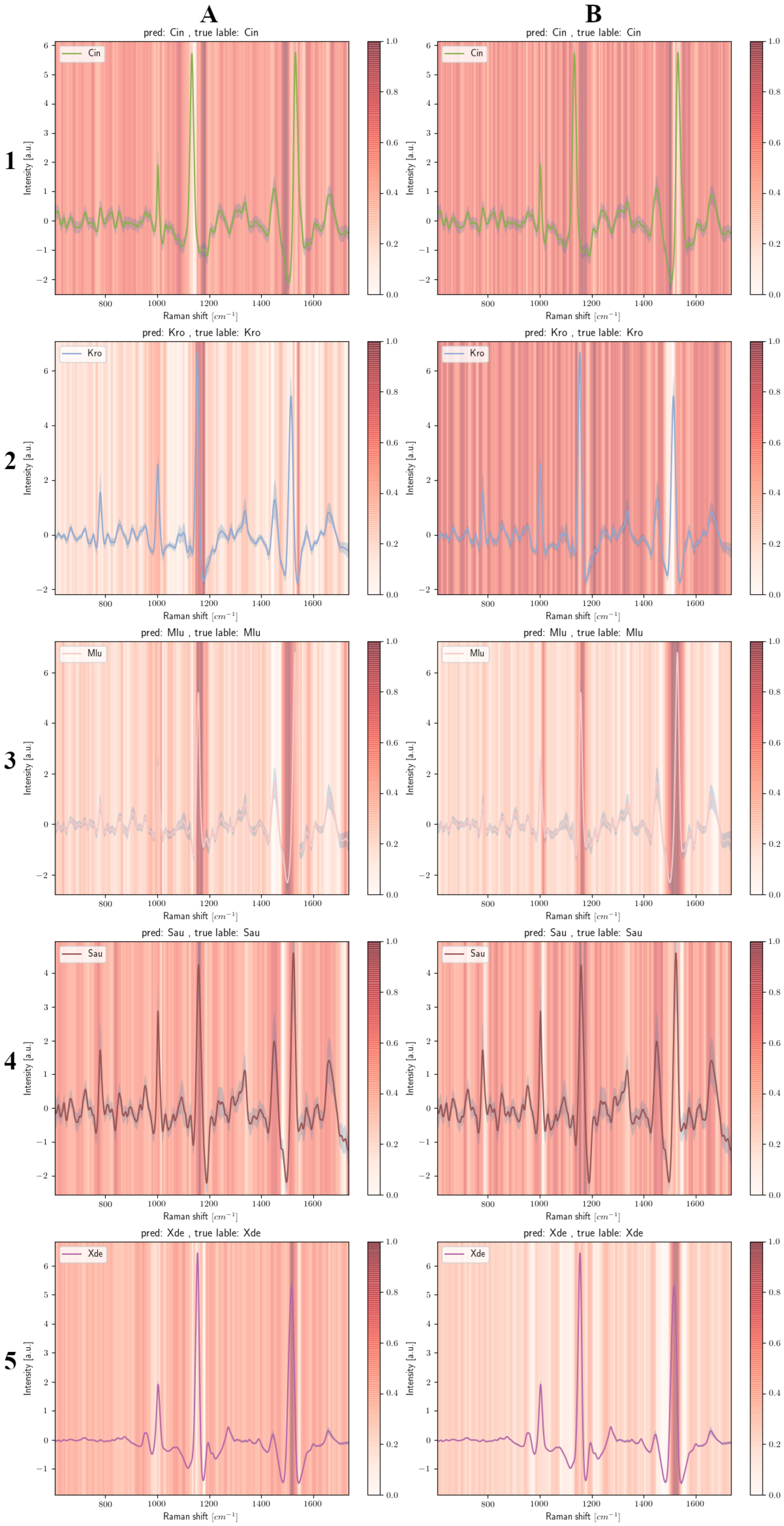
3.4.2. Carotenoid-Containing Microorganisms

The bands at about 1133 and 1530 cm−1, which are caused by the carotenoids in Cin, remain largely irrelevant by the CNN in model 1 (Figure 5(A1)) and also in model 2 (Figure 5(B1)). The negative slope at about 1504 cm−1, but also the quite neutral region at about 1176 cm−1 is of high importance for the CNN.
Particularly striking when comparing the Grad-CAM highlights of Kro (Figure 5A,B)) is the nearly opposite markings. In model 1, it is mainly the peak at about 1154 cm−1 and the short area thereafter, as well as the short negative slope at about 1538 cm−1 that are marked in deep red by the Grad-CAM, whereas all other spectral regions are hardly significant (Figure 5(A2)). In model 2, almost all regions are significant for the CNN except for the carotenoid band at about 1513 cm−1.
The Grad-CAM markings for Mlu (Figure 5(A3,B3) shows that especially areas near the carotenoid peaks are of interest for the CNN, whereas in model 1 (Figure 5(A3)), it is the area before the peak at about 1528 cm−1 that is important for the CNN. A short spectral region after the peak at about >1003 cm−1 also receives attention in the classification of Mlu, whereas the peak itself (caused by phenylalanine (Phe) [29]) is of less importance for the CNN.
At Sau, both models have a large number of areas marked by the Grad-CAM (Figure 5(A4,B4)). Noticeable in model 1 is the omission of the negative slope at about 1496 cm−1, whereas in model 2, the area after the Phe peak at about 1003 cm−1 is omitted (Figure 5(B4)). Conversely, the peak at about 781 cm−1, which is caused by a phosphate bond, cytosine, uracil, or thymine [7,30] is not very important for model 2 (Figure 5(B4)), but is more strongly marked for model 1 (Figure 5(A4)). Most important for the classification of Sau, however, are the signals associated with carotenoid at about 1158 cm−1.
Although the dense cluster of Xde in the PCA from Figure 3b suggests a simple distinction, many regions are important for the CNN in model 1 (Figure 5(A5)). The Grad-CAM markers for Xde of the second model (Figure 5(B5)) assign much less attention to most areas than model 1, and it is especially the strongly pronounced peak at about 1516 cm−1 that enables the classification there.
Contrary to what one might expect, it is not exclusively the very characteristic bands triggered by carotenoids that are used for differentiation, but also completely different areas within the spectra. Since these carotenoid-caused peaks differ significantly in wavenumber (e.g., Cin: 1530 cm−1, Kro 1514 cm−1, Mlu: 1528 cm−1, Sau: 1522 cm−1, Xde: 1516 cm−1), a predictive model might also succeed if it used only these features. So here, the CNN decides rather unintuitively.

4. Conclusions

It is widely accepted that it is the differences in the biochemical composition of different microorganisms that lead to different Raman spectra and thus to possible differentiability. This statement can of course be confirmed by the authors. Nevertheless, our quick look into such predictive models via Grad-CAM has shown that it is often not clear signatures that enable classification, but rather often minor nuances that make the difference. This work shows that models with identical data and training parameters can use completely different spectral regions for differentiation of the classes (microorganisms). CNN predictive models always take those features from the data that minimize their loss [31]. This may in some cases affect features that human experts would also use, but if there is another or an easier way to minimize the loss, CNN may use completely different spectral areas. Our results suggest that anthropomorphizing CNN models is dangerous because the networks often make unintuitive decisions that may be very different from human procedures, making the use of methods such as Grad-CAM important.

Supplementary Materials

The following supporting information can be downloaded at: https://www.mdpi.com/article/10.3390/ai4010006/s1. Figure S1: Mean Raman spectra of fungal spores Cb16III, Ca8II, Cb15, Mpemp, Bbass and normalized Grad-CAM indicator of CNN used signatures using a different baseline subtraction procedure as in the actual publication.

Author Contributions

T.J.T. conceptualized, elaborated the methodology, performed the experiments, analyzed the data and prepared the manuscript; D.P.B. conceptualized, supervised the study, and reviewed the document; M.C.W. elaborated the mathematical methodology, analyzed the data and reviewed and edited the document; B.T.H. performed experiments and reviewed the document; K.S.T. reviewed and edited the document; S.P. did literature research and reviewed the document; F.P. developed parts of the MATLAB codes and reviewed the document. All authors have read and agreed to the published version of the manuscript.

Funding

This research received no external funding.

Institutional Review Board Statement

Not applicable.

Informed Consent Statement

Not applicable.

Data Availability Statement

Not applicable.

Conflicts of Interest

The authors declare no conflict of interest.

References

  1. Stöckel, S.; Kirchhoff, J.; Neugebauer, U.; Rösch, P.; Popp, J. The application of Raman spectroscopy for the detection and identification of microorganisms. J. Raman Spectrosc. 2016, 47, 89–109. [Google Scholar] [CrossRef]
  2. Rösch, P.; Harz, M.; Krause, M.; Popp, J. Fast and reliable identification of microorganisms by means of Raman spectroscopy. In Biophotonics 2007: Optics in Life Science; Optical Society of America: Washington, DC, USA, 2007; pp. 6633–6645. [Google Scholar]
  3. Pahlow, S.; Meisel, S.; Cialla-May, D.; Weber, K.; Rösch, P.; Popp, J. Isolation and identification of bacteria by means of Raman spectroscopy. Adv. Drug Deliv. Rev. 2015, 89, 105–120. [Google Scholar] [CrossRef] [PubMed]
  4. Ho, C.S.; Jean, N.; Hogan, C.A.; Blackmon, L.; Jeffrey, S.S.; Holodniy, M.; Banaei, N.; Saleh, A.A.; Ermon, S.; Dionne, J. Rapid identification of pathogenic bacteria using Raman spectroscopy and deep learning. Nat. Commun. 2019, 10, 4927. [Google Scholar] [CrossRef] [PubMed] [Green Version]
  5. Meisel, S.; Stöckel, S.; Elschner, M.; Melzer, F.; Rösch, P.; Popp, J. Raman spectroscopy as a potential tool for detection of Brucella spp. in milk. Appl. Environ. Microbiol. 2012, 78, 5575–5583. [Google Scholar] [CrossRef] [Green Version]
  6. Rösch, P.; Harz, M.; Schmitt, M.; Peschke, K.D.; Ronneberger, O.; Burkhardt, H.; Motzkus, H.W.; Lankers, M.; Hofer, S.; Thiele, H.; et al. Chemotaxonomic identification of single bacteria by micro-Raman spectroscopy: Application to clean-room-relevant biological contaminations. Appl. Environ. Microbiol. 2005, 71, 1626–1637. [Google Scholar] [CrossRef] [Green Version]
  7. Strola, S.A.; Baritaux, J.-C.; Schultz, E.; Simon, A.C.; Allier, C.; Espagnon, I.; Jary, D.; Dinten, J.M. Single bacteria identification by Raman spectroscopy. J. Biomed. Opt. 2014, 19, 111610. [Google Scholar] [CrossRef]
  8. Hetjens, B.T.; Tewes, T.J.; Platte, F.; Wichern, F. The application of Raman spectroscopy in identifying Metarhizium brunneum, Metarhizium pemphigi and Beauveria bassiana. Biocontrol Sci. Technol. 2021, 32, 329–340. [Google Scholar] [CrossRef]
  9. Tewes, T.J.; Kerst, M.; Platte, F.; Bockmühl, D.P. Raman Microscopic Identification of Microorganisms on Metal Surfaces via Support Vector Machines. Microorganisms 2022, 10, 556. [Google Scholar] [CrossRef]
  10. Kanno, N.; Kato, S.; Ohkuma, M.; Matsui, M.; Iwasaki, W.; Shigeto, S. Machine learning-assisted single-cell Raman fingerprinting for in situ and nondestructive classification of prokaryotes. iScience 2021, 24, 102975. [Google Scholar] [CrossRef]
  11. Harz, M.; Rösch, P.; Popp, J. Vibrational spectroscopy-A powerful tool for the rapid identification of microbial cells at the single-cell level. Cytom. Part A 2009, 75, 104–113. [Google Scholar] [CrossRef]
  12. Mlynáriková, K.; Samek, O.; Bernatová, S.; Růžička, F.; Ježek, J.; Hároniková, A.; Šiler, M.; Zemánek, P.; Holá, V. Influence of culture media on microbial fingerprints using raman spectroscopy. Sensors 2015, 15, 29635–29647. [Google Scholar] [CrossRef] [Green Version]
  13. Harz, M.; Rösch, P.; Peschke, K.D.; Ronneberger, O.; Burkhardt, H.; Popp, J. Micro-Raman spectroscopic identification of bacterial cells of the genus Staphylococcus and dependence on their cultivation conditions. Analyst 2005, 130, 1543–1550. [Google Scholar] [CrossRef] [PubMed]
  14. Hutsebaut, D.; Maquelin, K.; De Vos, P.; Vandenabeele, P.; Moens, L.; Puppels, G.J. Effect of Culture Conditions on the Achievable Taxonomic Resolution of Raman Spectroscopy Disclosed by Three Bacillus Species. Anal. Chem. 2004, 76, 6274–6281. [Google Scholar] [CrossRef] [PubMed]
  15. Bocklitz, T.; Walter, A.; Hartmann, K.; Rösch, P.; Popp, J. How to pre-process Raman spectra for reliable and stable models? Anal. Chim. Acta 2011, 704, 47–56. [Google Scholar] [CrossRef] [PubMed]
  16. Schumacher, W.; Stöckel, S.; Rösch, P.; Popp, J. Improving chemometric results by optimizing the dimension reduction for Raman spectral data sets. J. Raman Spectrosc. 2014, 45, 930–940. [Google Scholar] [CrossRef]
  17. Kumar, B.N.V.; Kampe, B.; Rösch, P.; Popp, J. Characterization of carotenoids in soil bacteria and investigation of their photodegradation by UVA radiation via resonance Raman spectroscopy. Analyst 2015, 140, 4584–4593. [Google Scholar] [CrossRef]
  18. Burkart, N.; Huber, M.F. A survey on the explainability of supervised machine learning. J. Artif. Intell. Res. 2021, 70, 245–317. [Google Scholar] [CrossRef]
  19. Goodwin, N.L.; Nilsson, S.R.O.; Choong, J.J.; Golden, S.A. Toward the explainability, transparency, and universality of machine learning for behavioral classification in neuroscience. Curr. Opin. Neurobiol. 2022, 73, 102544. [Google Scholar] [CrossRef]
  20. Vinogradova, K.; Dibrov, A.; Myers, G. Towards Interpretable Semantic Segmentation via Gradient-Weighted Class Activation Mapping (Student Abstract). Proc. AAAI Conf. Artif. Intell. 2020, 34, 13943–13944. [Google Scholar] [CrossRef]
  21. Selvaraju, R.R.; Cogswell, M.; Das, A.; Vedantam, R.; Parikh, D.; Batra, D. Grad-cam: Why did you say that? Visual explanations from deep networks via gradient-based localization. Revista do Hospital das Clínicas 2016, 17, 331–336. [Google Scholar]
  22. Tewes, T.J.; Centeleghe, I.; Maillard, J.-Y.; Platte, F.; Bockmühl, D.P. Raman Microscopic Analysis of Dry-Surface Biofilms on Clinically Relevant Materials. Microorganisms 2022, 10, 1369. [Google Scholar] [CrossRef] [PubMed]
  23. Bradski, G. The OpenCV Library. Dr. Dobb’s J. Softw. Tools 2000, 120, 122–125. [Google Scholar]
  24. Gautam, R.; Vanga, S.; Ariese, F.; Umapathy, S. Review of multidimensional data processing approaches for Raman and infrared spectroscopy. EPJ Tech. Instrum. 2015, 2, 8. [Google Scholar] [CrossRef] [Green Version]
  25. Guo, S.; Popp, J.; Bocklitz, T. Chemometric analysis in Raman spectroscopy from experimental design to machine learning–based modeling. Nat. Protoc. 2021, 16, 5426–5459. [Google Scholar] [CrossRef]
  26. Chang, W.-C. On Using Principal Components Before Separating a Mixture of Two Multivariate Normal Distributions. J. R. Stat. Soc. Ser. C 1983, 32, 267–275. [Google Scholar] [CrossRef]
  27. De Siqueira e Oliveira, F.S.; Giana, H.E.; Silveira, L. Discrimination of selected species of pathogenic bacteria using near-infrared Raman spectroscopy and principal components analysis. J. Biomed. Opt. 2012, 17, 107004. [Google Scholar] [CrossRef]
  28. Huang, Z.; Lui, H.; Chen, M.X.; Alajlan, A.; McLean, D.I.; Zeng, H. Raman spectroscopy of in vivo cutaneous melanin. J. Biomed. Opt. 2004, 9, 1198–1205. [Google Scholar] [CrossRef]
  29. De Gelder, J.; De Gussem, K.; Vandenabeele, P.; Moens, L. Reference database of Raman spectra of biological molecules. J. Raman Spectrosc. 2007, 38, 1133–1147. [Google Scholar] [CrossRef]
  30. Schuster, K.C.; Reese, I.; Urlaub, E.; Gapes, J.R.; Lendl, B. Multidimensional Information on the Chemical Composition of Single Bacterial Cells by Confocal Raman Microspectroscopy. Anal. Chem. 2000, 72, 5529–5534. [Google Scholar] [CrossRef]
  31. Goodfellow, I.; Bengio, Y.; Courville, A. Deep Learning; MIT Press: Cambridge, MA, USA, 2016. [Google Scholar]
Figure 1. All Raman spectra of the fungal spores in grey and arithmetic mean spectra highlighted in black (displayed with a Y-axis offset). Untreated-but-normalized Raman spectra (a) and preprocessed spectra (baseline subtraction, smoothing, z-score normalization) (b).
Ai 04 00006 g001
Figure 2. All Raman spectra of the carotenoid-containing microorganisms in grey and arithmetic mean spectra highlighted in black (displayed with a Y-axis offset). Untreated-but-normalized Raman spectra (a) and preprocessed spectra (baseline subtraction, smoothing, z-score normalization) (b).
Ai 04 00006 g002
Figure 3. First three PCs of a PCA with the pretreated Raman spectra of the fungal spores (a) and carotenoid-containing microorganisms (b).
Ai 04 00006 g003
Figure 4. Mean Raman spectra of fungal spores Cb16III (A1), Ca8II (A2), Cb15 (A3), Mpemp(A4), Bbass (A5) and normalized Grad-CAM indicator of CNN used signatures of model 1. Mean Raman spectra of fungal spores Cb16III (B1), Ca8II (B2), Cb15 (B3), Mpemp (B4), Bbass (B5) and normalized Grad-CAM indicator of CNN used signatures of model 2. Z-score normalized Raman intensities on the Y-axis and Grad-CAM indicator normalized from zero to one (white to dark red).
Ai 04 00006 g004
Figure 5. Mean Raman spectra of carotenoid-containing microorganisms Cin (A1), Kro (A2), Mlu (A3), Sau (A4), Xde (A5) and normalized Grad-CAM indicator of CNN used signatures of model 1. Mean Raman spectra of carotenoid-containing microorganisms Cin (B1), Kro (B2), Mlu (B3), Sau (B4), Xde (B5) and normalized Grad-CAM indicator of CNN used signatures of model 2. Z-score normalized Raman intensities on the Y-axis and Grad-CAM indicator normalized from zero to one (white to dark red).
Ai 04 00006 g005
Table 1. All used fungal spores and carotenoid-containing microorganisms.
MicroorganismAbbreviationNumber of Spectra
Fungal sporesMetarhizium brunneum Cb16IIICb16III642
Metarhizium brunneum Ca8IICa8II562
Metarhizium brunneum Cb15IIICb15III525
Metarhizium pemphigi X1cMpemp847
Beauveria bassianaBbass372
Carotenoid-
containing
Chryseobacterium indolgenesCin684
Kocuria roseaKro639
Micrococcus luteusMlu1842
Staphylococcus aureusSau1094
Xanthophyllomyces dendrorhousXde658
Table 2. Precision, recall, F1 score and support with model 1 for fungal spores.
MicroorganismPrecisionRecallF1-ScoreSupport
Cb16III0.980.970.97131
Ca8II0.880.830.86133
Cb150.960.970.96105
Mpemp0.890.920.90181
Bbass1.001.000.9974
accuracy 0.93624
macro avg0.940.930.94624
weighted avg0.930.930.93624
Table 3. Precision, recall, F1 score and support with model 2 for fungal spores.
MicroorganismPrecisionRecallF1-ScoreSupport
Cb16III0.970.980.98131
Ca8II0.900.820.85133
Cb150.980.970.97105
Mpemp0.870.930.90181
Bbass1.001.000.9974
accuracy 0.93624
macro avg0.940.940.94624
weighted avg0.930.930.93624
Table 4. Precision, recall, F1 score and support with model 1 for carotenoid-containing microorganisms.
MicroorganismPrecisionRecallF1-ScoreSupport
Cin1.001.001.00137
Kro1.001.001.00128
Mlu1.001.001.00368
Sau1.001.001.00219
Xde1.001.001.00130
accuracy 1.00983
macro avg1.001.001.00983
weighted avg1.001.001.00983
Table 5. Precision, recall, F1 score and support with model 2 for carotenoid-containing microorganisms.
MicroorganismPrecisionRecallF1-ScoreSupport
Cin1.001.001.00137
Kro1.001.001.00128
Mlu1.001.001.00368
Sau1.001.001.00219
Xde1.001.001.00130
accuracy 1.00983
macro avg1.001.001.00983
weighted avg1.001.001.00983
Disclaimer/Publisher’s Note: The statements, opinions and data contained in all publications are solely those of the individual author(s) and contributor(s) and not of MDPI and/or the editor(s). MDPI and/or the editor(s) disclaim responsibility for any injury to people or property resulting from any ideas, methods, instructions or products referred to in the content.

