Article

A General Hybrid Modeling Framework for Systems Biology Applications: Combining Mechanistic Knowledge with Deep Neural Networks under the SBML Standard

LAQV-REQUIMTE, Department of Chemistry, NOVA School of Science and Technology, NOVA University Lisbon, Campus da Caparica, 2829-516 Caparica, Portugal
*
Author to whom correspondence should be addressed.
AI 2023, 4(1), 303-318; https://doi.org/10.3390/ai4010014
Submission received: 31 January 2023 / Revised: 15 February 2023 / Accepted: 27 February 2023 / Published: 1 March 2023
(This article belongs to the Special Issue Feature Papers for AI)

Abstract

:
In this paper, a computational framework is proposed that merges mechanistic modeling with deep neural networks obeying the Systems Biology Markup Language (SBML) standard. Over the last 20 years, the systems biology community has developed a large number of mechanistic models that are currently stored in public databases in SBML. With the proposed framework, existing SBML models may be redesigned into hybrid systems through the incorporation of deep neural networks into the model core, using a freely available python tool. The so-formed hybrid mechanistic/neural network models are trained with a deep learning algorithm based on the adaptive moment estimation method (ADAM), stochastic regularization and semidirect sensitivity equations. The trained hybrid models are encoded in SBML and uploaded in model databases, where they may be further analyzed as regular SBML models. This approach is illustrated with three well-known case studies: the Escherichia coli threonine synthesis model, the P58IPK signal transduction model, and the Yeast glycolytic oscillations model. The proposed framework is expected to greatly facilitate the widespread use of hybrid modeling techniques for systems biology applications.

Graphical Abstract

1. Introduction

Hybrid modeling methods combining mechanistic knowledge with machine learning (ML) in a common workflow have found wide application in process systems engineering since the early 1990s (e.g., review by von Stosch et al., [1]). Psichogios and Ungar [2] described one of the first applications of hybrid models to bioprocess engineering. The proposed hybrid model consisted of dynamic material balance equations of biochemical species (system of ordinary differential equations (ODEs)) connected with a shallow feed-forward neural network in a common mathematical structure. Sensitivity equations were derived enabling the training of the neural network by error backpropagation on indirect training examples (e.g., measured target variables not coincident with the neural network output variables). Thompson and Kramer [3] framed this problem as hybrid semiparametric modeling, as such models merge parametric functions (stemming from knowledge) with nonparametric functions (stemming from data) in the same mathematical structure. Schubert et al. [4] presented the first industrial application of hybrid modeling (material balance equations combined with neural networks) to a Baker’s yeast process. Since the early 1990s, hybrid model structure definition, parameter identification and model-based process control have been extensively covered (e.g., [5,6,7,8,9,10]). Hybrid models were applied to a wide array of microbial, animal cells, mixed microbial and enzyme processes in different industries, such as wastewater treatment, clean energy, biopolymers and biopharmaceutical manufacturing (Agharafeie et al. [11]). The potential advantages of hybrid modeling may be summarized as a more rational usage of prior knowledge (mechanistic, heuristic and empirical) eventually translating into more accurate, transparent and robust process models [7,10].
With a significant lag, hybrid modeling is currently receiving a lot of attention in the systems biology scientific community. ML has been applied for the prediction of the function of genes [12] and proteins [13] and is gaining popularity in all fields of systems biology [14]. Cuperlovic-Culf et al. [15] highlighted the difficulty of gathering high-quality in vivo data to validate detailed metabolic models, and the opportunity to alternatively apply ML and hybrid mechanistic/ML methods. Antonakoudis et al. [16] recently reviewed the efforts to integrate GEnome-scale Models (GEMs) with supervised and unsupervised ML. Kim et al. [17] reviewed ML applications in the construction and simulation of GEMs, and ML applications in use of GEM-derived information. The integration of mechanistic models and ML may be realized through a hybrid pipeline of activities, where both modeling frameworks participate to solve particular sub-tasks. Alternatively, mechanistic and ML models may be “fused” in a common semiparametric mathematical structure. Following the latter approach, hybrid metabolic flux analysis, combining metabolic networks and principal component analysis (PCA) in semiparametric linear models, has been studied by Carinhas et al. [18] and Isidro et al. [19]. Hybrid metabolic models combining metabolic networks and partial least squares have been proposed by Ferreira et al. [20] and Teixeira et al. [21]. The combination of systems of ODEs with neural networks (hybrid ODEs formalism) for the modeling of biochemical networks with intrinsic time delays has been studied by von Stosch et al. [22]. The integration of elementary flux modes (EMs) and PCA for hybrid metabolic pathway analysis has been researched by Folch-Fortuny et al. [23] and von Stosch et al. [24]. Hybrid dynamic models that combine ODEs, PCA and EMs have been addressed by Folch-Fortuny et al. [23]. Lee et al. [25] developed hybrid mechanistic/neural network models for partially known intracellular signaling pathways. Hybrid modeling approaches combining neural networks and ODEs have been applied to describe immunodeficiency virus (HIV) dynamics [26] and coronavirus disease 2019 (COVID-19) dynamics [27]. Yang et al. [28] developed a white-box machine learning approach, leveraging carefully curated biological network models to mechanistically link input and output data, to reveal metabolic mechanisms of antibiotic lethality. Lewis and Kemp [29] applied genome-scale flux balance analysis (FBA) to generate data to train ML classifiers to predict tumor radiosensitivity. Vijayakumar et al. [30] developed a hybrid pipeline combining multi-omics ML with genome-scale FBA to analyze the phenotypic potential of cyanobacterium. Ramos et al. [31] recently proposed a hybrid FBA technique that integrates GEMs and PCA constraints in a common linear program with mechanistic decision variables (fluxes) concomitantly with empirical decision variables (scores of principal components).
A large number of systems biology models, including GEMs, have been developed and stored in databases (e.g., BioModels [32], JWS online [33], and KiMoSys [34]) in the Systems Biology Markup Language (SBML) format [35]. SBML is a free and open standard based on XML to encode computational models of biological processes with widespread use in the systems biology scientific community. The SBML standard is, however, not commonly adopted in ML software tools. This significantly hinders the interlink between both modeling approaches in a hybrid workflow. Here, we propose a hybrid modeling framework that combines both modeling approaches obeying to the SBML standard. A previously published python package, SBML2HYB, is used to convert existing systems biology models into hybrid models and vice versa [36]. The so-formed hybrid models are trained with a deep learning algorithm based on ADAM, stochastic regularization and semidirect sensitivity equations [37]. The final (trained) hybrid models are uploaded in SBML databases, where they may be further analyzed as regular SBML models. This procedure was applied to three well-known models: the E. coli threonine pathway model [38], the P58IPK signal transduction pathway model [39] and the yeast glycolytic oscillations model [40].

2. Methods

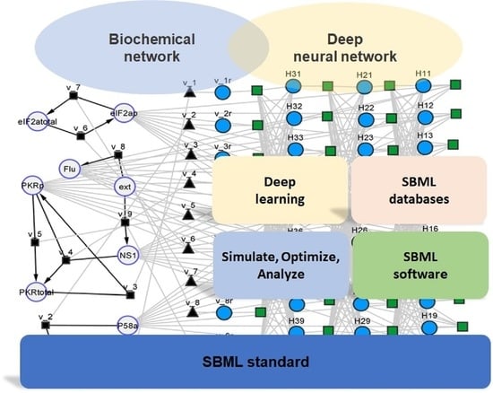
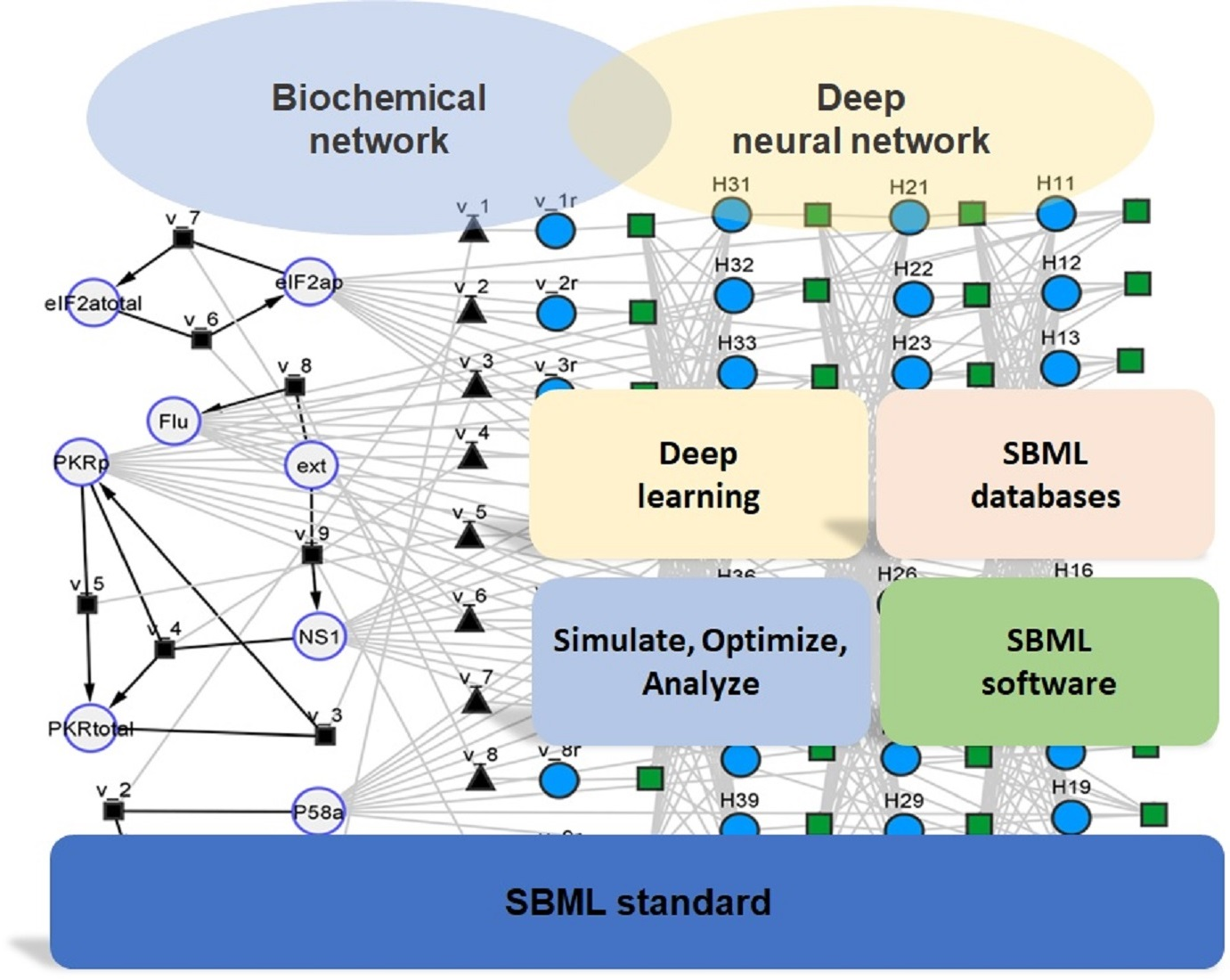
2.1. General SBML Hybrid Model

SBML models are organized as j = 1, …, n compartments with size V j . Each compartment contains   m j species with a concentration vector c j . The species are interlinked through q j reactions with stoichiometry S j and reaction kinetics r j . SBML models also contain parameters, θ, with given initial values (parameters may be local to reactions or global; for simplicity, we assume global). In SBML, the parameter values are not necessarily fixed as they may change over time according to predefined algebraic rules. The compartment size may also change over time according to predefined compartment rate rules (other rate rules were not considered here for simplicity). External time dependent stimuli may be defined through events, giving rise to a vector of exogenous input variables, u , that may change over time. With these elements, the dynamics of biochemical species in a generic compartment j may be described by the following ODEs model:
d c j V j d t = S j × r j c j , θ , u , ϑ , t × V j
d V j d t = z j V j , c j , θ , u , ϑ , t
θ = h V j , c j , θ , u , ϑ , t
Equation (1a) is a conservation law of mass assuming a perfectly mixed compartment. Equation (1b) represents a generic compartment rate rule in case the compartment size changes over time. Equation (1c) represents generic algebraic rules to compute model parameters over time. Equations (1a)–(1c) are of a parametric nature with fixed structure stemming from prior knowledge (e.g., mass conservation laws, reaction stoichiometry or enzyme kinetics). Some variables may, however, lack a mechanistic basis (e.g., unknown reaction kinetics mechanisms or unknown physicochemical properties of molecular species such as charge or glycosylation pattern). In the general SBML hybrid model, variables lacking a mechanistic basis are defined as loose nonparametric functions, ϑ(∙), without a fixed structure. They are computed by a deep feedforward neural network (FFNN) with n h hidden layers as a function of species concentrations, exogenous inputs, and other relevant variables:
H 0 = g V j , c j , θ , u , t
H i = σ   w i · H i 1 + b i , i = 1 , ,   n h  
ϑ · = w n h + 1 · H n h + b n h + 1
A non-linear pre-processing function, g( V j , cj, θ, u, t), may be used to compute the FFNN input signals to improve the training (Equation (2a)). The input signals are forward propagated through the hidden layers according to Equation (2b). The σ(∙) represents the nodes transfer function in the hidden layers (always the hyperbolic tangent function in this study). Finally, the FNN outputs, ϑ, are computed by a linear output layer (Equation (2c)). The nodes connections weights, w = w 1 , w 2 , , w n h + 1 and b = b 1 , b 2 , , b n h + 1 , are calculated during the training of the model, for which an informative dataset is needed.
For a particular biological model, Equations (1)–(2) describing n compartments with species and reactions are transformed via automatic symbolic manipulation into an equivalent set of ODEs and derived sensitivity equations using the Symbolic Math toolbox (MATLAB R2020a, MathWorks Inc.). The end result of this procedure is an automatically generated Matlab/Octave function that computes time derivatives of all state variables, y = { c 1 ,     c 2 , , c n ,     V 1 ,   V 2 , , V n } ,
d y d t = f y , ϑ , u , t
and also the semidirect sensitivity parameters obtained by the symbolic differentiation of Equation (3a) with respect to state variables, y, and FFNN outputs, ϑ,
d y ϑ d t = f y y ϑ + f ϑ
y ϑ | t = 0 = 0
Deep learning of hybrid models obeying to the system of Equations (3a)–(3c) has been thoroughly investigated by Pinto et al. [37]. A Runge–Kutta 4th order ODE solver was implemented in MATLAB R2020a (MathWorks Inc.) to integrate the system of Equations (3a)–(3c). The training was performed in a weighted least squares sense by minimizing the following loss function,
W M S E = 1 T   t = 1 T ( y t * y t ) 2   σ t 2  
with T the number of training examples, y t * the measured training example at time t, y t the corresponding model prediction and σ t the measurement standard deviation. The gradients of the loss function with respect to the neural network outputs were computed by the equation,
W M S E ϑ = 2   t = 1 T y t * y t σ i 2 y ϑ t
The output layer gradients, W M S E / ϑ , were back-propagated to the input layer via the well-known error backpropagation algorithm (Werbos, 1974), yielding the loss function gradients with respect to the neural network parameters,
g = W M S E ω , W M S E b
Finally, the adaptive moment estimation algorithm (ADAM) [41] with stochastic minibatch and weights dropout regularization was adopted to minimize the loss function given by Equation (4), using gradients, g . For further details, the reader is referred to [25]. The code was implemented in MATLAB R2020a (MathWorks Inc.) on a computer with Intel® CoreTM i5–8265U CPU @ 1.60 GHz 1.80 GHz, and 24 GB of RAM.

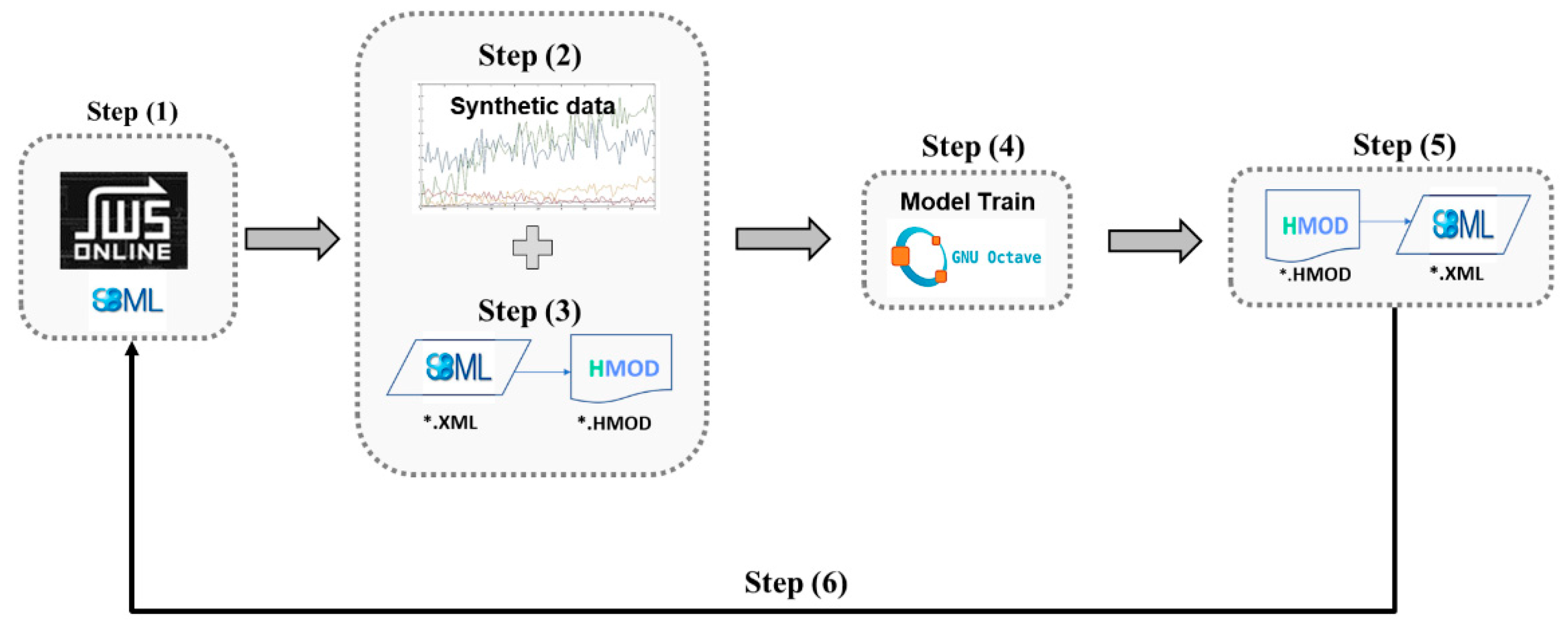
2.2. Interfacing with SBML Databases and SBML Modeling Tools

The SBML2HYB python package [36] was adopted to read SBML models, redesign them as hybrid models and to store them in model databases. This freely available python package converts existing systems biology models encoded in SBML into hybrid models that combine mechanistic equations and deep neural networks (currently limited to FFNNs). SBML is not a common format to encode ML models. An intermediate HMOD format supports the conversion process. The HMOD format is a text-based file (ASCII) with the list of properties defining the model (species, reactions, parameters, rates and rules) in a similar manner to SBML, by considering any number of species with a certain initial concentration distributed among any number of compartments. These species are then interlinked through a list of reactions and rate rules. The user inputs the information of the deep neural network into the HMOD file either manually or through a pre-configured neural network in Python keras, using the SBML2HYB tool. The resulting hybrid model in HMOD format is reconverted to SBML and uploaded in model databases. In this step, the FFNN Equations (2a)–(2c) are mapped to assignment rules in SBML format, whereas the network weights are mapped to global parameters in the SBML format. The resulting SBML hybrid models may be simulated, analyzed and/or trained with existing tools such as MATLAB (MathWorks Inc.), COPASI [42] or special purpose tools with training algorithms for hybrid models that are able to read SBML files. For further details, the reader is referred to [36].

2.3. Case Studies

The SBML hybrid modeling framework was applied to three systems biology case studies freely available in the JWS Online database (https://jjj.bio.vu.nl/models/, accessed on 31 January 2023) [33] with the accession ID given in Table 1. The first case study is a metabolic network describing the synthesis of threonine in E. coli proposed by Chassagnole et al. [38]. The second case study is the P58IPK signal transduction network to study Influenza infection dynamics proposed by Goodman et al. [39]. The third case study is a reduced yeast glycolytic model with preserved limit cycle stability proposed by Dano et al. [40]. In order to upgrade the original mechanistic models in hybrid mechanistic/neural network versions, the following pipeline of activities (Figure 1) was applied to each of the case studies:
Step 1: The original systems biology models were retrieved from the JWS database in SBML format. The respective files are provided as Supplementary Material.
Step 2: Synthetic time series datasets were generated by simulating the original models in the JWS platform. The resulting data sets are provided as Supplementary Material. These data are needed to train the hybrid models as a proof-of-concept. No experimental data were used in this study. More details are provided in the results section.
Step 3: For each case study, a feedforward neural network (FFNN) was inserted into the mechanistic model and converted to the HMOD format using the SBML2HYB python tool, freely available in [36]. The size of the FFNN and interface with the mechanistic model depended on the case study. More details are given in the results section.
Step 4: The hybrid mechanistic/FFNN models encoded in the HMOD format were trained using the deep learning approach described in Section 2.1 and the datasets generated in step 2. Implementation details varied in the case studies (more on this in the Results section). The main concern was the proof-of-concept that SBML hybrid models may be efficiently trained to a comparable performance to the original mechanistic models. The effect of the size of the FFNN was investigated. The final trained hybrid models, with the updated FFNN weights, were saved in the HMOD format.
Step 5: The trained hybrid models in the HMOD format were reconverted to SBML using the SBML2HYB tool. In this step, the FFNN information is mapped to assignment rules in the SBML format. The obtained SBML files were uploaded to the JWS online platform and are now freely available for the community to analyze. The hybrid model structures encoded in SBML were visualized using the freely available Cytoscape cy3sbml tool [43]. The hybrid models SBML files are provided as Supplementary Material.
Step 6: For proof-of-concept, the original mechanistic SBML models (step 1) and the final hybrid SBML models (step 5) were simulated and compared using the JWS online simulator (https://jjj.bio.vu.nl/models/experiments/, accessed on 31 January 2023) showing that their outputs are practically coincident.
As mentioned in step 5, hybrid models with different network depths and sizes were evaluated for each case study. The “best” hybrid model was discriminated on the basis of the Akaike Information Criterion with a second order bias correction (AICc), computed for the training data partition as follows:
A I C c = T   l n + 2   n w + 2   n w   n w + 1 T n w 1
with n w the total number of FFNN weights that are calculated during the training process. AICc includes an overparameterization penalty and is commonly used to discriminate between empirical model candidates and to select a parsimonious model for small sample sizes [44].

3. Results and Discussion

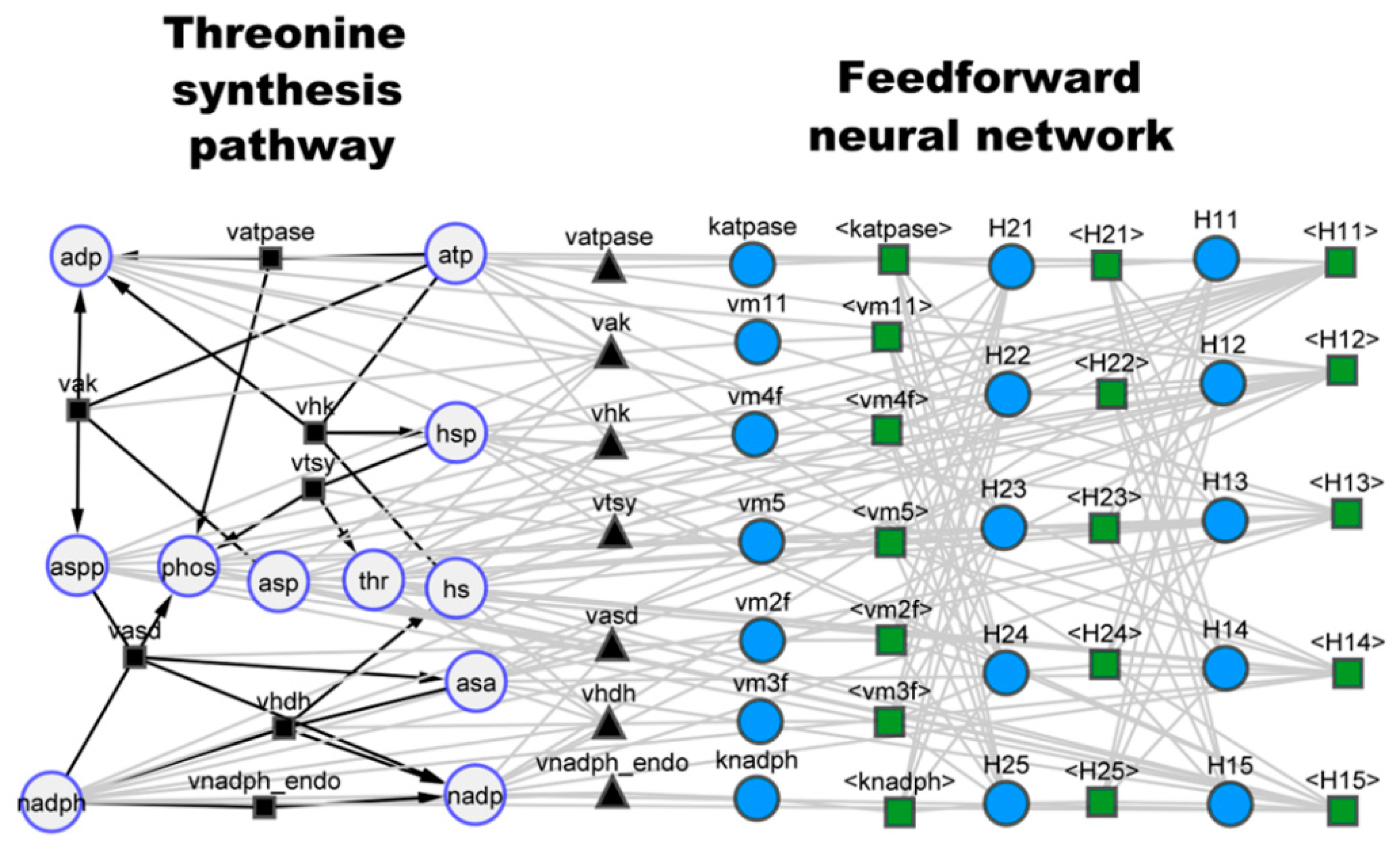
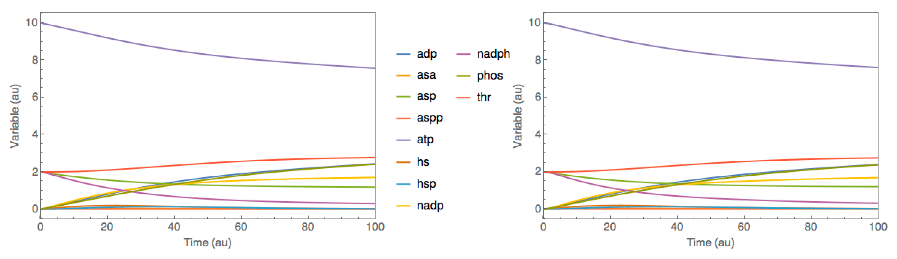
3.1. Case Study 1: Threonine Synthesis Pathway in E. coli

The first case study is the metabolic model proposed by Chassagnole et al. [38], describing the threonine synthesis pathway in E. coli (Table 1). This model dynamically simulates the time course of 11 species (adp, asa, asp, aspp, atp, hs, hsp, nadp, naph, phos and thr) in a single compartment, corresponding to 11 ODEs. It has seven reactions (with rates vak, vasd, vatpase, vhdh, vhk, vnadph_endo and vtsy) and 47 kinetic parameters (the names of variables were kept the same as in the original SBML model to facilitate cross-reference; for details, the reader is referred to the JWS Online model with accession ID ‘chassagnole’).
Hybrid models were created by combining deep FFNNs of different sizes with the original mechanistic model, following the previously described procedure (Figure 1). The FFNNs had 11 inputs corresponding to the concentrations of the 11 species (adp, asa, asp, aspp, atp, hs, hsp, nadp, naph, phos, thr). The number of hidden layers and nodes in the hidden layers varied (Table 2). The activation function in the hidden layers was always the hyperbolic tangent function. The FFNNs had seven outputs corresponding to the maximum reaction rate values of the seven metabolic reactions. The kinetic equations of the original SBML model were fully kept in the hybrid models. The job of the FFNNs was thus to describe the maximum reaction rate parameters as a function of species concentrations. Figure 2 graphically represents the hybrid model structure [11 × 5 × 5 × 7] (Table 2) using the Cytoscape cy3sbml tool. This figure shows an heterogenous (hybrid) network composed of nodes and edges of different nature. On the biochemical network side (left), the large circles represent the molecular species, which have a physical concentration associated. The small black squares and respective edges represent biochemical reactions with a well-defined stoichiometry. The black triangles are the reaction kinetic rates. On the feedforward neural network side (right), the blue circles represent the neural network nodes, which have an abstract numerical value associated defining the node strength. The green squares and respective edges represent signal propagation between nodes. The interlink between the two sides of the network is mediated by the black triangles, which in this case correspond to the maximum reaction rate parameters to be applied in the kinetic law equations. An interesting analogy may be established between the neural network part and an artificial nucleus of a cell with associated signal transduction networks and gene regulatory networks, with the job of controlling the underlying metabolic processes.
The hybrid models were trained with a synthetic data set following the procedure of Figure 1. A time series dataset was created by simulating the original SBML model directly in the JWS platform. A two-factor central composite design of experiments (CC-DOE) was carried out to the initial concentrations of atp between 5 and 15 (arbitrary units) and of asp between 1 and 3 (arbitrary units) resulting in nine experiments. The data for each experiment was recorded as a time series with 100 data points and a sampling time of 1 (arbitrary units). Gaussian noise (10%) was added to concentrations of species, thereby simulating experimental error. This synthetic dataset is available in the Supplementary Material (Simulation_data.xlsx; chassagnole_data sheet). From the nine experiments, four were used for training (the star experiments of the CC-DOE corresponding to 400 training examples for each state variable) and five were used for testing (the square plus the center experiments of the CC-DOE corresponding to 500 training examples for each state variable). The training was performed with ADAM with default hyperparameters (Table 2), 5000 iterations, semidirect sensitivity equations and stochastic regularization with a minibatch size of 0.78 and weights dropout of 0.22. The choice of the minibatch size and weights dropout was based on the results by Pinto et al. [37]. Table 2 shows the overall training metrics for different FFNNs sizes. The performances of the hybrid models in terms of training error (WMSE train) and testing error (WMSE test) are comparable. The magnitude of the train and test errors are also comparable, denoting an effective training without overfitting in all cases. This is further strengthened by the very low noise-free test error showing that model predictions are very close to the true process behavior in all cases. The total number of network weights varied almost 10-fold but this was not reflected in the training performance. The best hybrid structure was chosen to be the smallest one [11 × 5 × 5 × 7] based on the lowest AICc value (1st row in Table 2).
The trained hybrid models may be simulated and analyzed in any systems biology platform complying with the SBML standard. As proof-of-concept, the best hybrid model [11 × 5 × 5 × 7] in the SBML format was uploaded to the JWS online platform and simulated. Figure 3 shows the JWS online simulation of the original model and of the best hybrid model [11 × 5 × 5 × 7] for a test experiment not used for training (the center point experiment of the CC-DOE). The results show that the hybrid model perfectly mimicked the dynamics of the original mechanistic model.
The procedure presented in Figure 1 may result in mathematical structures that are more detailed mechanistically and much more complex to train than previously published hybrid models. This may raise concerns about the training feasibility of FFNNs interlinked with complex mathematical structures. Pinto et al. [37] compared traditional shallow hybrid modeling (using the Levenberg–Marquardt algorithm coupled with the indirect sensitivity equations, cross-validation and a hyperbolic tangent activation function) with deep hybrid modeling (using ADAM, semidirect sensitivity equations, stochastic regularization and multiple hidden layers). A clear advantage of hybrid deep learning both in terms of predictive power and computational cost was demonstrated. However, all experiments had a simplistic mechanistic part. Here, case study 1 model kept the original kinetic law equations. Seven highly complex kinetic equations with 47 parameters were “merged” with the FFNN. Table 2 results suggest nonetheless that the previously published deep learning approach for hybrid models (ADAM + semidirect sensitivity equations + stochastic regularization) is equally effective at training hybrid models with complex parametric functions.

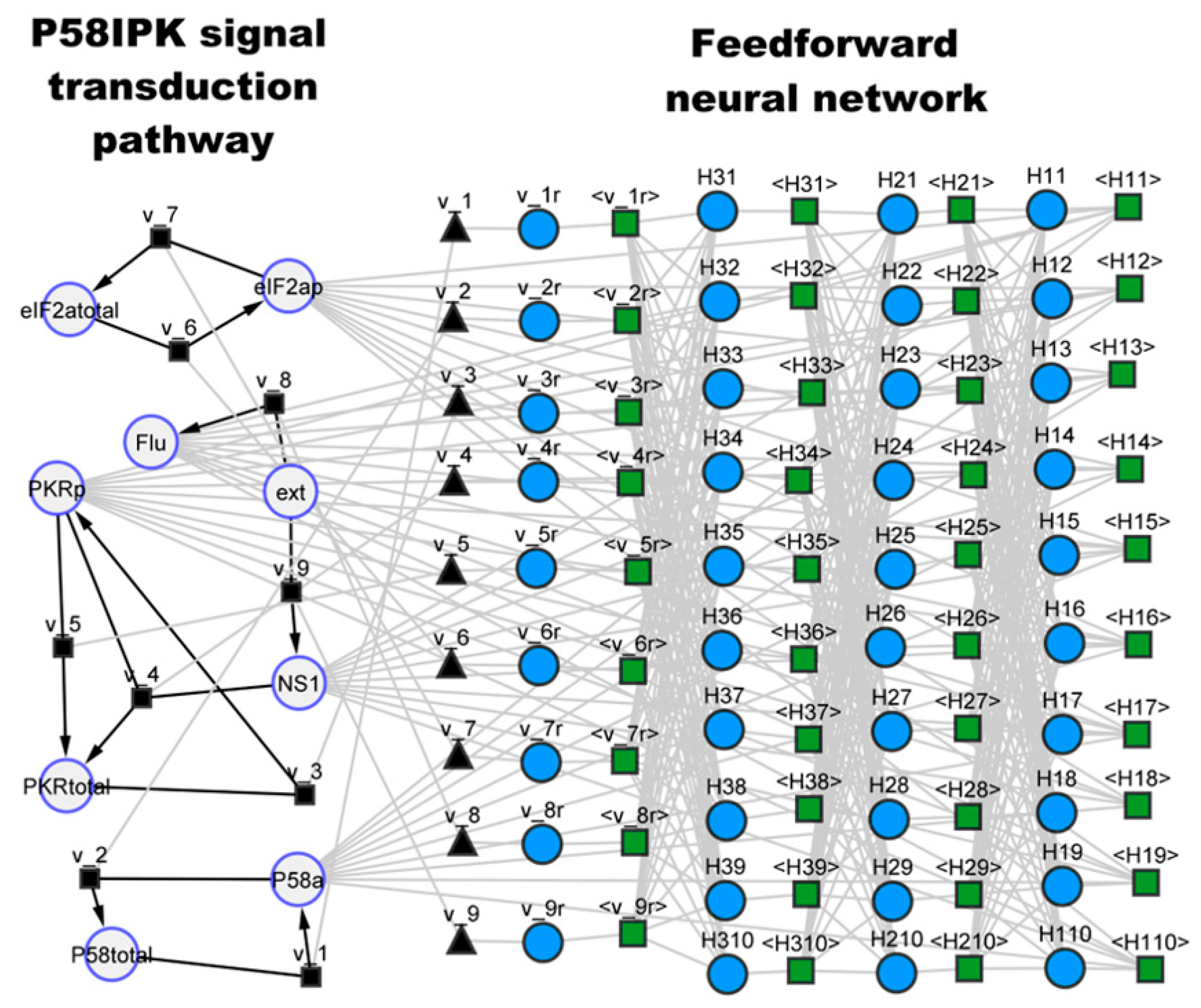
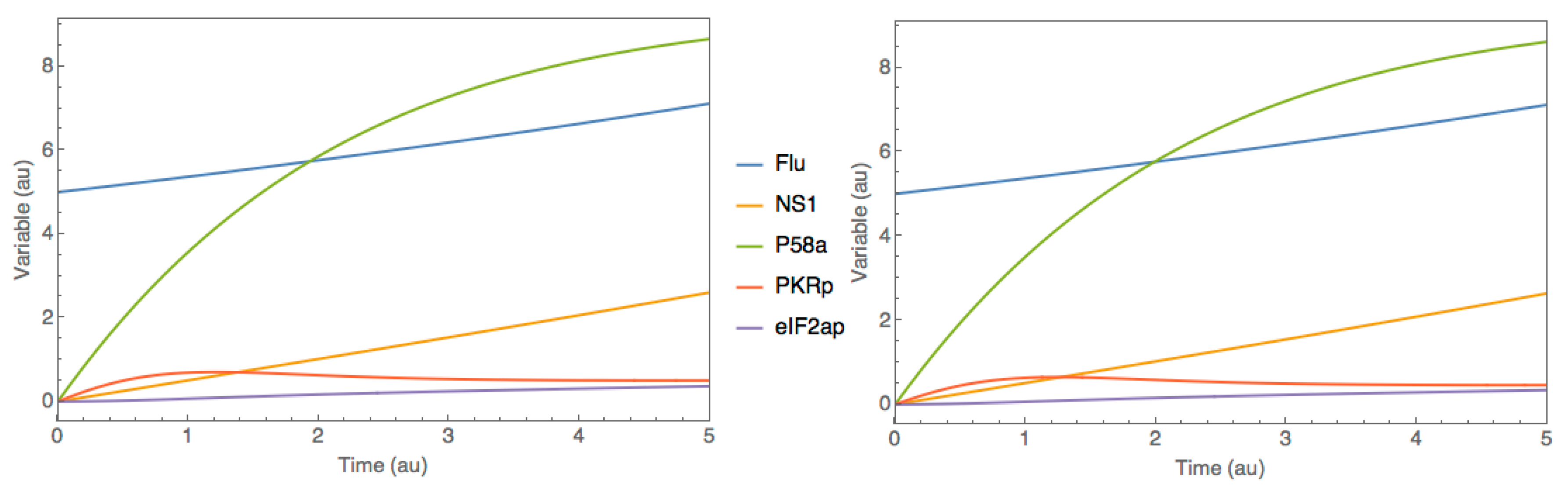
3.2. Case Study 2: P58IPK Signal Transduction Pathway

The second case study was based on the viral infection model proposed by Goodman et al. [39], freely available in SBML in the JWS Online database (http://www.jjj.bio.vu.nl, accessed on 31 January 2023) under accession ID ‘goodman’ (Table 1). The authors studied the dynamics of the P58IPK signal transduction pathway during Influenza virus infection. A mathematical model was developed to evaluate the effect of protein P58a activation on the P58IPK pathway dynamics, particularly on the activation of the PKR kinase and on the phosphorylation of eIF2, both controlling viral protein expression. The model comprehends nine species (Flu, NS1, P58a, P58total, PKRp, PKRtotal, eIF2ap, eIF2atotal and ext) in a single compartment, of which four are fixed (P48total, PKRtotal, eIF2atotal and ext), corresponding to five ODEs. The model further has nine reactions and 10 parameters. The names of variables were kept the same as in the original model and are explained in the database.
As in the previous case study, SBML hybrid models were created by combining FFNNs of different sizes (Table 3) with the original mechanistic model following the procedure of Figure 1. Figure 4 shows the hybrid model structure [5 × 10 × 10 × 10 × 9] (Table 3) using the SBML-visualizing cy3sbml tool [43]. The left side of Figure 4 represents the original mechanistic signal transduction network, whereas the right side represents the FFNN added to the mechanistic core. The FFNN has five inputs corresponding to the concentrations of the five dynamical species (Flu, NS1, P58a, PKRp and EIF2ap), three hidden layers (10 × 10 × 10) with hyperbolic tangent activation functions, and nine outputs corresponding to the kinetic rates (v_1r, v_2r, v_3r, v_4r, v_5r, v_6r, v_7r, v_8r, v_9r as they are named in the original SBML implementation). In this case study, the FFNNs in Table 3 completely replaced the kinetic laws of the original model, which were therefore deleted in the hybrid model structures. This network may be interpreted as a hybrid signal transduction pathway with a physical part composed of proteins and an artificial part composed of abstract neural network nodes.
Hybrid SBML models with varying number of hidden layers and nodes in the hidden layers were trained using a synthetic data set. A time-series dataset was created by simulating the original SBML model in the JWS platform following a similar procedure to case study 1 (available in the Supplementary Material as Simulation_data.xlsx; goodman_data sheet). A two-factor CC-DOE was carried out to the initial amount of Flu (overall level of infection within the host cell) between 2 and 6 (arbitrary units) and the initial amount of PKRp (phosphorylated PKR protein) between 0 and 2 (arbitrary units). The data for each experiment were recorded as a time series with 100 points and sampling time of 0.05 (arbitrary units). This resulted in nine experiments with 100 time points each. Additionally, 10% Gaussian noise was added to concentrations of species to simulate experimental error. As in the previous case study, four experiments were selected for training (the star experiments of the CC-DOE corresponding to 400 training examples for each state variable) and five experiments were used for testing (the square plus the center experiments of the CC-DOE corresponding to 500 training examples for each state variable). The training was performed using ADAM with default hyperparameters (Table 3), 5000 iterations, semidirect sensitivity equations and stochastic regularization (minibatch size of 0.78 and weight dropout of 0.22, as before). The overall training results for different FFNN sizes are shown in Table 3. As opposed to the previous case study, the size of the FFNN has an effect on the training performance. This may be explained by the smaller amount of mechanistic knowledge embodied in the hybrid models. Since the original kinetic laws were completely deleted in the hybrid models, the training results are more heavily dependent on the FFNN structure. Interestingly, the larger networks with a higher depth (three hidden layers) outperformed the smaller networks, particularly in the extrapolation experiments (test WMSE). Overall, the structure [5 × 10 × 10 × 10 × 9] stands out as the best-performing model with the lowest training error (WMSE train) and lowest testing error (WMSE test). This is further reinforced by the lowest noise-free test error and the lowest AICc. This structure was uploaded to the JWS online platform and simulated comparatively to the original mechanistic model (Figure 5). As in the previous case study, the best-performing hybrid SBML model [5 × 10 × 10 × 10 × 9] was able to perfectly mimic the dynamics of the original mechanistic model.

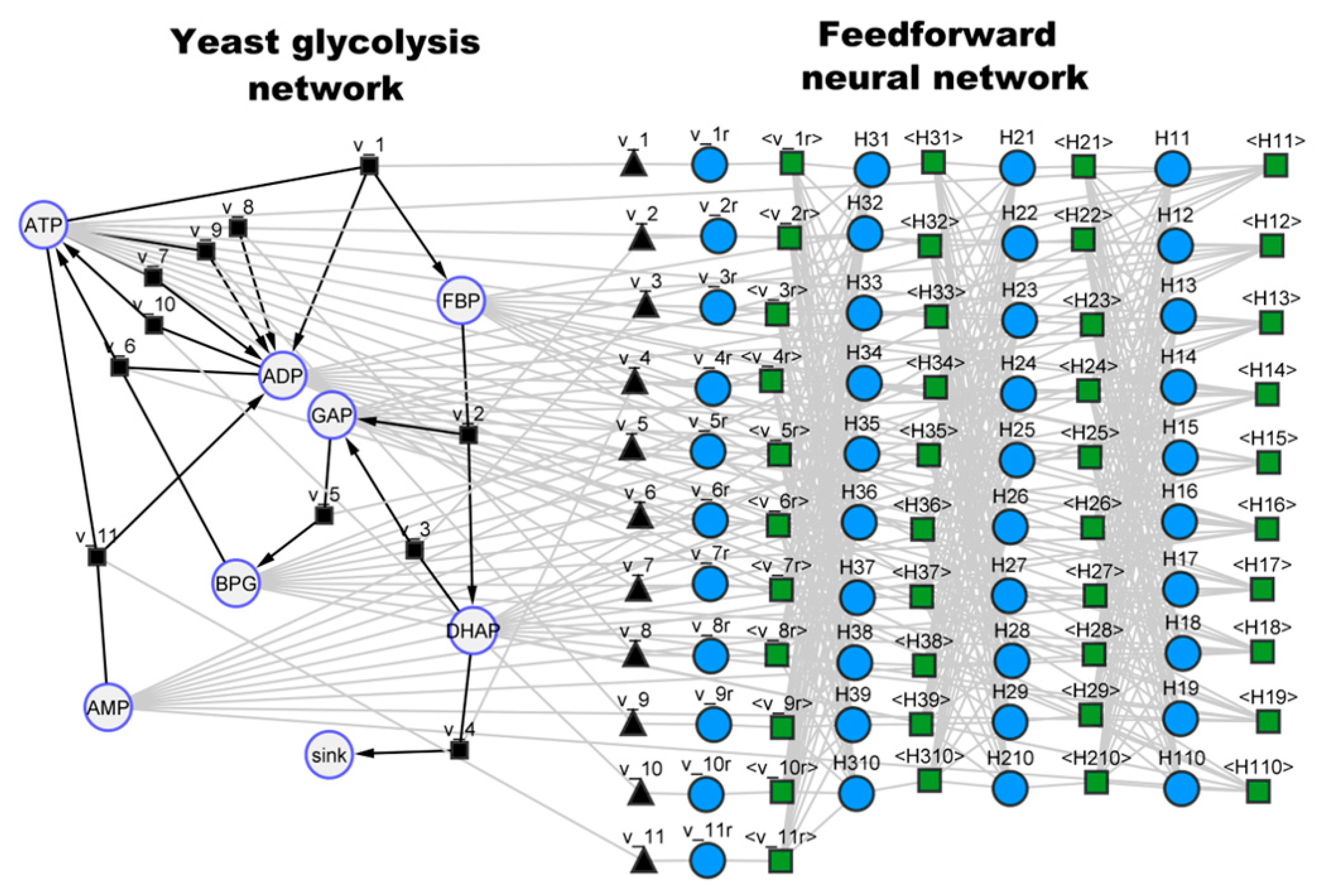
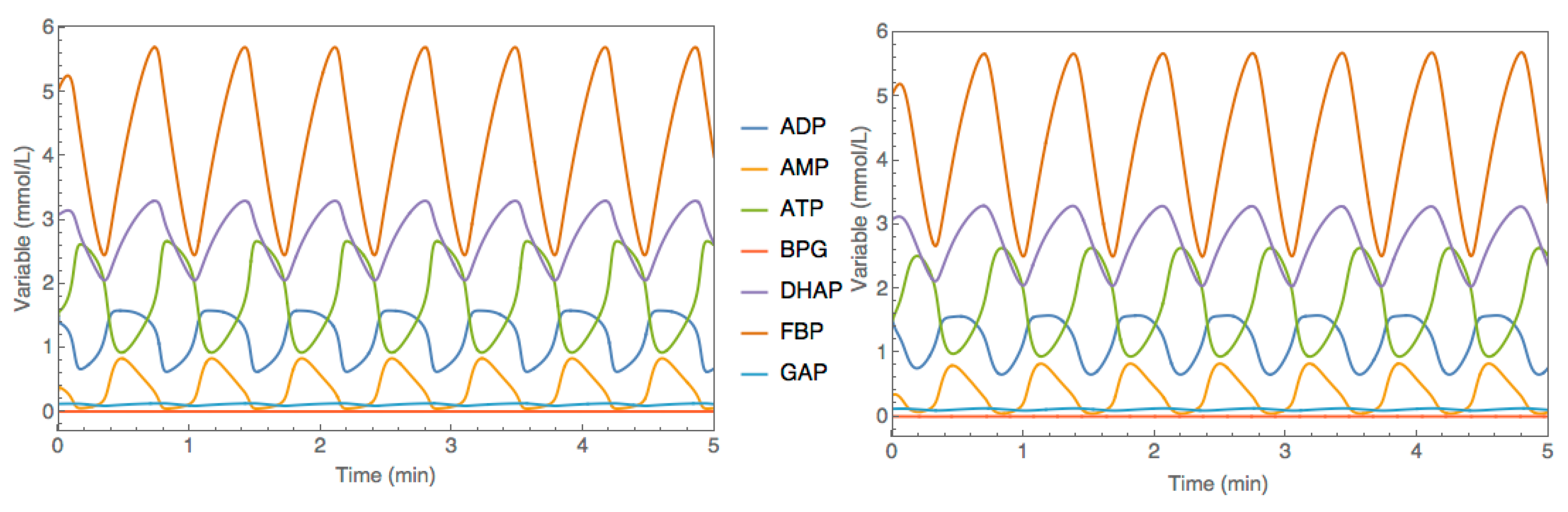
3.3. Case Study 3: Yeast Glycolytic Oscillations

The third case study consisted of the reduced dynamical model of yeast glycolysis proposed by Dano et al. [40]. This model is a reduced version of a more detailed yeast glycolysis model. Both the original and reduced models exhibit limit cycle stability, with a certain number of species showing stable oscillations over time. It comprehends eight species (ADP, AMP, ATP, BPG, DHAP, FBP, GAP and sink) in a single compartment. The dynamic variable ‘sink’ was the only one that was fixed, thus translating to a system of seven ODEs. The model further comprehends 11 metabolic reactions and 31 parameters. This model is freely available in SBML format on the JWS Online database (http://www.jjj.bio.vu.nl, accessed on 31 January 2023) with accession ID ‘dano1′.
SBML hybrid models were created by combining FFNNs of different sizes with the original mechanistic model. Figure 6 illustrates this process for the structure [7 × 10 × 10 × 10 × 11] with 421 weights (6th row of Table 4). The right side of Figure 6 represents the original metabolic network, whereas the left side represents the incorporated FFNN. In this example, the FFNN has seven inputs corresponding to the concentrations of the seven species (ADP, AMP, ATP, BPG, DHAP, FBP, GAP), three hidden layers (10 × 10 × 10) with hyperbolic tangent activation functions, and 11 outputs corresponding to the kinetic rates (v_1r, v_2r, v_3r, v_4r, v_5r, v_6r, v_7r, v_8r, v_9r, v_10r, v_11r as they are named in the original SBML model). As in case study 2, the original kinetic laws were completely deleted in the hybrid models.
Hybrid SBML models of different sizes were trained with a synthetic dataset following a similar process to the previous case studies. A two-factor CC-DOE was carried out by varying the amount of initial ADP concentration between 1 and 2 (arbitrary units) and the initial ATP concentration between 1 and 2 (arbitrary units), resulting in nine experiments. Each experiment was simulated on the JWS Online platform with the resulting time-series data (100 time points) recorded with a sampling time of 0.05 (arbitrary units). Gaussian noise (10%) was added to the concentrations of species. This synthetic dataset is available as Supplementary Material (Simulation_data.xlsx; dano1_data sheet). Four experiments were selected for training (the star experiments of the CC-DOE corresponding to 400 training examples for each state variable) and five were used for testing (the square plus the center experiments of the CC-DOE corresponding to 500 training examples for each state variable). The hybrid models were trained with this data using ADAM with default hyperparameters (10,000 iterations, semidirect sensitivity equations, stochastic regularization with minibatch size of 0.78 and weight dropout of 0.22). The overall training results for different FFNNs sizes are shown in Table 4. Unsurprisingly, limit cycle stability is a more challenging problem for hybrid model development. The effect of the FFNN depth and size was much more pronounced than in the previous example. The smaller networks were not able to exhibit stable oscillations even for the training examples. Only models with three hidden layers were able to accurately capture the oscillatory dynamics. The three largest structures show a comparable training and testing error. However, the structure [7 × 10 × 10 × 10 × 11] clearly stands out as the best-performing model with the lowest training error (WMSE train) and the lowest testing error (WMSE test). This is further accentuated by the significantly lower noise-free test error and lower AICc. This hybrid SBML model was uploaded to the JWS online platform and simulated comparatively to the original metabolic model for the center point test experiment (not used for training) of the CC-DOE (Figure 7). Remarkably, the best hybrid model structure [7 × 10 × 10 × 10 × 11] was able to reproduce very faithfully the oscillatory behavior of the original metabolic model when exposed to different initial conditions than those applied in the training experiments.

4. Conclusions

SBML is an open standard based on XML currently adopted by the systems biology community to encode computational models of biological processes. An extensive body of research has produced a large number of such SBML models that are currently stored in public databases. The SBML standard is, however, not commonly adopted to encode ML models. The main novelty of the present study is the combination of both modeling formalisms in a common hybrid workflow obeying the SBML standard. With few exceptions, previously published hybrid models embodied relatively simple mechanistic models (mechanistic scale-gap) and relatively simple ML models (ML scale-gap). With the proposed SBML hybrid modeling framework, the mechanistic scale-gap may be significantly narrowed. It is shown with three simple examples how publicly available SBML models may be easily upgraded to hybrid mechanistic/neural network models obeying the SBML standard. Such hybrid models may be trained with state-of-the-art deep learning algorithms to either mimic, improve or extend existing SBML models. They may be further uploaded, trained and analyzed in SBML compatible software tools. Even if the presented examples are relatively simple, the proposed framework is, in principle, directly scalable to larger whole organism models, eventually at the genome-scale. All in all, we expect this framework to greatly facilitate the adoption of hybrid mechanistic/ML techniques to develop computational models of biological systems.

Supplementary Materials

The following supporting information can be downloaded at: https://www.mdpi.com/article/10.3390/ai4010014/s1, Synthetic datasets for the 3 case studies: Simulation_data.xlsx. Case study 1: threonine synthesis model in E. coli: SBML file of original mechanistic model: chassagnole1.xml, SBML file of hybrid mechanistic/FFNN model: chassagnole1hyb.xml, JWS Online ID of hybrid mechanistic/FFNN model: pinto1; Case study 2: P58IPK signal transduction pathway: SBML file of original mechanistic model: goodman.xml, SBML file of hybrid mechanistic/FFNN model: goodmanhyb.xml, JWS Online ID of hybrid mechanistic/FFNN model: pinto2; Case study 3: Yeast glycolytic oscillations: SBML file of original mechanistic model: dano1.xml, SBML file of hybrid mechanistic/FFNN model: dano1hyb.xml, JWS Online ID of hybrid mechanistic/FFNN model: pinto3.

Author Contributions

Conceptualization, J.P., R.S.C. and R.O.; methodology, J.P., R.S.C. and R.O.; software, J.P.; investigation, J.P.; data curation, J.P.; writing—original draft preparation, J.P.; writing—review and editing, J.R.C.R., R.S.C. and R.O.; supervision, R.O. All authors have read and agreed to the published version of the manuscript.

Funding

This work was supported by the Associate Laboratory for Green Chemistry—LAQV which is financed by national funds from FCT/MCTES (UIDB/50006/2020 and UIDP/50006/2020). This work has received funding from the European Union’s Horizon 2020 research and innovation program under grant agreement number 870292 (BioICEP project). J.P. acknowledges a PhD grant (SFRD/BD14610472019), Fundação para a Ciência e Tecnologia (FCT) and R.S.C. the contract CEECIND/01399/2017.

Institutional Review Board Statement

Not applicable.

Informed Consent Statement

Not applicable.

Data Availability Statement

The data presented in this study are available in Supplementary Material.

Conflicts of Interest

The authors declare no conflict of interest.

References

  1. von Stosch, M.; Oliveira, R.; Peres, J.; de Azevedo, S.F. Hybrid semi-parametric modeling in process systems engineering: Past, present and future. Comput. Chem. Eng. 2014, 60, 86–101. [Google Scholar] [CrossRef] [Green Version]
  2. Psichogios, D.C.; Ungar, L.H. A Hybrid Neural Network-1st Principles Approach to Process Modeling. Aiche J. 1992, 38, 1499–1511. [Google Scholar] [CrossRef]
  3. Thompson, M.L.; Kramer, M.A. Modeling Chemical Processes Using Prior Knowledge and Neural Networks. Aiche J. 1994, 40, 1328–1340. [Google Scholar] [CrossRef]
  4. Schubert, J.; Simutis, R.; Dors, M.; Havlik, I.; Lubbert, A. Hybrid Modeling of Yeast Production Processes—Combination of a-Priori Knowledge on Different Levels of Sophistication. Chem. Eng. Technol. 1994, 17, 10–20. [Google Scholar] [CrossRef]
  5. Teixeira, A.P.; Clemente, J.J.; Cunha, A.E.; Carrondo, M.J.T.; Oliveira, R. Bioprocess iterative batch-to-batch optimization based on hybrid parametric/nonparametric models. Biotechnol. Prog. 2006, 22, 247–258. [Google Scholar] [CrossRef] [PubMed]
  6. Teixeira, A.P.; Alves, C.; Alves, P.M.; Carrondo, M.J.; Oliveira, R. Hybrid elementary flux analysis/nonparametric modeling: Application for bioprocess control. BMC Bioinform. 2007, 8, 30. [Google Scholar] [CrossRef] [PubMed] [Green Version]
  7. von Stosch, M.; Oliveira, R.; Peres, J.; de Azevedo, S.F. A novel identification method for hybrid (N)PLS dynamical systems with application to bioprocesses. Expert Syst. Appl. 2011, 38, 10862–10874. [Google Scholar] [CrossRef]
  8. Pinto, J.; de Azevedo, C.R.; Oliveira, R.; von Stosch, M. A bootstrap-aggregated hybrid semi-parametric modeling framework for bioprocess development. Bioprocess Biosyst. Eng. 2019, 42, 1853–1865. [Google Scholar] [CrossRef]
  9. Rajulapati, L.; Chinta, S.; Shyamala, B.; Rengaswamy, R. Integration of machine learning and first principles models. Aiche J. 2022, 68, e17715. [Google Scholar] [CrossRef]
  10. Glassey, J.; von Stosch, M. Hybrid Modeling in Process Industries, 1st ed.; Taylor&Francis, Ed.; CRC Press: Boca Raton, FL, USA, 2018. [Google Scholar]
  11. Agharafeie, R.; Oliveira, R.; Ramos, J.; Mendes, J. Application of Hybrid Neural Models to Bioprocesses: A Systematic Literature Review. Authorea 2023. [Google Scholar] [CrossRef]
  12. Le, N.Q.K.; Do, D.T.; Hung, T.N.K.; Lam, L.H.T.; Huynh, T.T.; Nguyen, N.T.K. A Computational Framework Based on Ensemble Deep Neural Networks for Essential Genes Identification. Int. J. Mol. Sci. 2020, 21, 9070. [Google Scholar] [CrossRef] [PubMed]
  13. Le, N.Q.K. Potential of deep representative learning features to interpret the sequence information in proteomics. Proteomics 2022, 22, e2100232. [Google Scholar] [CrossRef]
  14. Greener, J.G.; Kandathil, S.M.; Moffat, L.; Jones, D.T. A guide to machine learning for biologists. Nat. Rev. Mol. Cell Biol. 2022, 23, 40–55. [Google Scholar] [CrossRef]
  15. Cuperlovic-Culf, M.; Nguyen-Tran, T.; Bennett, S.A.L. Machine Learning and Hybrid Methods for Metabolic Pathway Modeling. Methods Mol. Biol. 2023, 2553, 417–439. [Google Scholar] [CrossRef] [PubMed]
  16. Antonakoudis, A.; Barbosa, R.; Kotidis, P.; Kontoravdi, C. The era of big data: Genome-scale modelling meets machine learning. Comput. Struct Biotec. 2020, 18, 3287–3300. [Google Scholar] [CrossRef] [PubMed]
  17. Kim, Y.; Kim, G.B.; Lee, S.Y. Machine learning applications in genome-scale metabolic modeling. Curr. Opin. Syst. Biol. 2021, 25, 42–49. [Google Scholar] [CrossRef]
  18. Carinhas, N.; Bernal, V.; Teixeira, A.P.; Carrondo, M.J.T.; Alves, P.M.; Oliveira, R. Hybrid metabolic flux analysis: Combining stoichiometric and statistical constraints to model the formation of complex recombinant products. BMC Syst. Biol. 2011, 5, 34. [Google Scholar] [CrossRef] [PubMed] [Green Version]
  19. Isidro, I.A.; Portela, R.M.; Clemente, J.J.; Cunha, A.E.; Oliveira, R. Hybrid metabolic flux analysis and recombinant protein prediction in Pichia pastoris X-33 cultures expressing a singlechain antibody fragment. Bioprocess Biosyst. Eng. 2016, 39, 1351–1363. [Google Scholar] [CrossRef]
  20. Ferreira, A.R.; Dias, J.M.L.; von Stosch, M.; Clemente, J.; Cunha, A.E.; Oliveira, R. Fast development of Pichia pastoris GS115 Mut(+) cultures employing batch-to-batch control and hybrid semi-parametric modeling. Bioprocess Biosyst. Eng. 2014, 37, 629–639. [Google Scholar] [CrossRef]
  21. Teixeira, A.P.; Dias, J.M.L.; Carinhas, N.; Sousa, M.; Clemente, J.J.; Cunha, A.E.; von Stosch, M.; Alves, P.M.; Carrondo, M.J.T.; Oliveira, R. Cell functional enviromics: Unravelling the function of environmental factors. BMC Syst. Biol. 2011, 5, 92. [Google Scholar] [CrossRef] [Green Version]
  22. von Stosch, M.; Peres, J.; de Azevedo, S.F.; Oliveira, R. Modelling biochemical networks with intrinsic time delays: A hybrid semi-parametric approach. BMC Syst. Biol. 2010, 4, 131. [Google Scholar] [CrossRef] [Green Version]
  23. Folch-Fortuny, A.; Marques, R.; Isidro, I.A.; Oliveira, R.; Ferrer, A. Principal elementary mode analysis (PEMA). Mol. Biosyst. 2016, 12, 737–746. [Google Scholar] [CrossRef] [PubMed] [Green Version]
  24. von Stosch, M.; Hamelink, J.M.; Oliveira, R. Hybrid modeling as a QbD/PAT tool in process development: An industrial E-coli case study. Bioprocess Biosyst. Eng. 2016, 39, 773–784. [Google Scholar] [CrossRef] [PubMed] [Green Version]
  25. Lee, D.; Jayaraman, A.; Kwon, J.S. Development of a hybrid model for a partially known intracellular signaling pathway through correction term estimation and neural network modeling. PLoS Comput. Biol. 2020, 16, e1008472. [Google Scholar] [CrossRef] [PubMed]
  26. Umar, M.; Sabir, Z.; Raja, M.A.Z.; Baskonus, H.M.; Yao, S.W.; Ilhan, E. A novel study of Morlet neural networks to solve the nonlinear HIV infection system of latently infected cells. Results Phys. 2021, 25, 104235. [Google Scholar] [CrossRef]
  27. Umar, M.; Sabir, Z.; Raja, M.A.Z.; Shoaib, M.; Gupta, M.; Sanchez, Y.G. A Stochastic Intelligent Computing with Neuro-Evolution Heuristics for Nonlinear SITR System of Novel COVID-19 Dynamics. Symmetry 2020, 12, 1628. [Google Scholar] [CrossRef]
  28. Yang, J.H.; Wright, S.N.; Hamblin, M.; McCloskey, D.; Alcantar, M.A.; Schrubbers, L.; Lopatkin, A.J.; Satish, S.; Nili, A.; Palsson, B.O.; et al. A White-Box Machine Learning Approach for Revealing Antibiotic Mechanisms of Action. Cell 2019, 177, 1649–1661.e9. [Google Scholar] [CrossRef]
  29. Lewis, J.E.; Kemp, M.L. Integration of machine learning and genome-scale metabolic modeling identifies multi-omics biomarkers for radiation resistance. Nat. Commun. 2021, 12, 2700. [Google Scholar] [CrossRef]
  30. Vijayakumar, S.; Rahman, P.K.S.M.; Angione, C. A Hybrid Flux Balance Analysis and Machine Learning Pipeline Elucidates Metabolic Adaptation in Cyanobacteria. Iscience 2020, 23, 101818. [Google Scholar] [CrossRef]
  31. Ramos, J.R.C.; Oliveira, G.P.; Dumas, P.; Oliveira, R. Genome-scale modeling of Chinese hamster ovary cells by hybrid semi-parametric flux balance analysis. Bioprocess Biosyst. Eng. 2022, 45, 1889–1904. [Google Scholar] [CrossRef]
  32. Le Novere, N.; Bornstein, B.; Broicher, A.; Courtot, M.; Donizelli, M.; Dharuri, H.; Li, L.; Sauro, H.; Schilstra, M.; Shapiro, B.; et al. BioModels Database: A free, centralized database of curated, published, quantitative kinetic models of biochemical and cellular systems. Nucleic Acids Res. 2006, 34, D689–D691. [Google Scholar] [CrossRef] [PubMed] [Green Version]
  33. Olivier, B.G.; Snoep, J.L. Web-based kinetic modelling using JWS Online. Bioinformatics 2004, 20, 2143–2144. [Google Scholar] [CrossRef] [PubMed] [Green Version]
  34. Mochao, H.; Barahona, P.; Costa, R.S. KiMoSys 2.0: An upgraded database for submitting, storing and accessing experimental data for kinetic modeling. Database J. Biol. Databases Curation 2020, 2020, baaa093. [Google Scholar] [CrossRef] [PubMed]
  35. Hucka, M.; Fineey, A.; Sauro, H.M.; Bolouri, H.; Doyle, J.C.; Kitano, H.; Arkin, A.P.; Bornstein, B.J.; Bray, D.; Cornish-Bowden, A.; et al. The systems biology markup language (SBML): A medium for representation and exchange of biochemical network models. Bioinformatics 2003, 19, 524–531. [Google Scholar] [CrossRef] [PubMed] [Green Version]
  36. Pinto, J.; Costa, R.S.; Alexandre, L.; Ramos, J.; Oliveira, R. SBML2HYB: A Python interface for SBML compatible hybrid modelling. Bioinformatics 2023, 39, btad044. [Google Scholar] [CrossRef] [PubMed]
  37. Pinto, J.; Mestre, M.; Ramos, J.; Costa, R.S.; Striedner, G.; Oliveira, R. A general deep hybrid model for bioreactor systems: Combining first principles with deep neural networks. Comput. Chem. Eng. 2022, 165, 107952. [Google Scholar] [CrossRef]
  38. Chassagnole, C.; Fell, D.A.; Rais, B.; Kudla, B.; Mazat, J.P. Control of the threonine-synthesis pathway in Escherichia coli: A theoretical and experimental approach. Biochem. J. 2001, 356, 433–444. [Google Scholar] [CrossRef] [PubMed]
  39. Goodman, A.G.; Tanner, B.C.W.; Chang, S.T.; Esteban, M.; Katze, M.G. Virus infection rapidly activates the P58(IPK) pathway, delaying peak kinase activation to enhance viral replication. Virology 2011, 417, 27–36. [Google Scholar] [CrossRef] [PubMed] [Green Version]
  40. Dano, S.; Madsen, M.F.; Schmidt, H.; Cedersund, G. Reduction of a biochemical model with preservation of its basic dynamic properties. Febs J. 2006, 273, 4862–4877. [Google Scholar] [CrossRef]
  41. Kingma, D.P.; Ba, J. Adam: A method for stochastic optimization. arxiv 2014, arXiv:1412.6980. [Google Scholar]
  42. Hoops, S.; Sahle, S.; Gauges, R.; Lee, C.; Pahle, J.; Simus, N.; Singhhal, M.; Xu, L.; Mendes, P.; Kummer, U. COPASI—A COmplex PAthway SImulator. Bioinformatics 2006, 22, 3067–3074. [Google Scholar] [CrossRef] [PubMed] [Green Version]
  43. Konig, M.; Drager, A.; Holzhutter, H.G. CySBML: A Cytoscape plugin for SBML. Bioinformatics 2012, 28, 2402–2403. [Google Scholar] [CrossRef] [PubMed] [Green Version]
  44. Li, B.B.; Morris, J.; Martin, E.B. Model selection for partial least squares regression. Chemom. Intell. Lab. 2002, 64, 79–89. [Google Scholar] [CrossRef]
Figure 1. Schematic workflow for redesigning existing SBML models stored in databases into hybrid mechanistic/neural network models. Step 1: An SBML biologic model is extracted from a model database. Step 2: A synthetic time series dataset is generated to train the hybrid model. Step 3: A feedforward neural network (FFNN) is inserted in the mechanistic kinetic model and converted to the HMOD format using the SBML2HYB tool. Step 4: The hybrid mechanistic/FFNN model encoded in the HMOD format is trained by applying the deep learning approach (Section 2.1) and the synthetic dataset. Step 5: The trained hybrid model in the HMOD format is reconverted to SBML using the SBML2HYB tool. Step 6: The final trained hybrid model in the SBML format is uploaded in the model database and simulated comparatively to the original nonhybrid model.
Ai 04 00014 g001
Figure 2. Hybrid model structure [11 × 5 × 5 × 7] for the threonine synthesis pathway (1st row of Table 2) visualized in the cy3sbml tool [43]. Left side: Metabolic network with physical meaning. Large circles represent biochemical species (metabolites). Black squares and black edges represent biochemical reactions. Black triangles represent kinetic laws. Right side: Artificial feedforward neural network with size [11 × 5 × 5 × 7]. Small blue circles represent neural network nodes. Green squares and gray edges represent signal propagation between neural network nodes. The first layer receives input signals of biochemical species concentrations (Large circles). The last layer delivers kinetic parameter values to the black triangles, which mediate the communication between both sides of the network.
Ai 04 00014 g002
Figure 3. Comparison between original model and best hybrid model for case study 1 (threonine synthesis pathway in E. coli) Dynamic profiles were simulated based on the respective SBML files in the JWS Online platform. The test experiment was the center point experiment of the CC-DOE (not used for training). Full lines represent species concentrations over time. Left panel: Original SBML model simulation. Right panel: Best hybrid model simulation with structure [11 × 5 × 5 × 7] (First row of Table 2).
Ai 04 00014 g003
Figure 4. Hybrid model structure [5 × 10 × 10 × 10 × 9] for the P58IPK signal transduction pathway (6th row of Table 3) visualized using the cy3sbml tool [43]. Left side: Signal transduction network with physical meaning. Large circles represent biochemical species (proteins). Black squares and black edges represent biochemical reactions. Black triangles represent kinetic laws. Right side: Artificial feedforward neural network with size [5 × 10 × 10 × 10 × 9]. Small blue circles represent neural network nodes. Green squares and gray edges represent signal propagation between neural network nodes. The first layer receives input signals of biochemical species concentrations (Large circles). The last layer delivers kinetic parameter values to the black triangles, which mediate the communication between both sides of the network.
Ai 04 00014 g004
Figure 5. Comparison between original model and best hybrid model for case study 2 (P58IPK signal transduction pathway). Dynamic profiles were simulated based on the respective SBML files in the JWS Online platform. The test experiment was the center point experiment of the CC-DOE (not used for training). Full lines represent species concentrations over time. Left panel: Original SBML model simulation. Right panel: Best hybrid model simulation with structure [5 × 10 × 10 × 10 × 9] (Sixth row of Table 3).
Ai 04 00014 g005
Figure 6. Hybrid model structure [7 × 10 × 10 × 10 × 11] for the yeast glycolysis pathway (6th row of Table 3) visualized in the cy3sbml tool [43]. Left side: Reduced glycolysis network with physical meaning. Large circles represent biochemical species (metabolites). Black squares and black edges represent biochemical reactions. Black triangles represent kinetic laws. Right side: Artificial feedforward neural network with size [7 × 10 × 10 × 10 × 11]. Small blue circles represent neural network nodes. Green squares and gray edges represent signal propagation between neural network nodes. The first layer receives input signals of biochemical species concentrations (Large circles). The last layer delivers kinetic parameter values to the black triangles, which mediate the communication between both sides of the network.
Ai 04 00014 g006
Figure 7. Comparison between original model and best hybrid model for case study 3 (yeast glycolysis model). Dynamic profiles were simulated based on the respective SBML files on the JWS Online platform. Simulations were performed for the center point experiment of the CC-DOE (not used for training). Full lines represent species concentrations over time. Left panel: Original SBML model simulation. Right panel: Best hybrid model simulation with structure [7 × 10 × 10 × 10 × 11] (Sixth row of Table 4).
Ai 04 00014 g007
Table 1. Summary of the three SBML models that were redesigned to hybrid mechanistic/neural network models in the present study.
Case StudyNumber of SpeciesNumber of ReactionsNumber of ParametersJWS Online IDReference
E. coli threonine synthesis pathway11747chassagnole1[38]
P58IPK signal transduction pathway9 (4 fixed)910goodman[39]
Yeast glycolytic oscillations7 (1 fixed)1131dano1[40]
Table 2. Training metrics of different hybrid models for the E. coli threonine synthesis pathway case study (chassagnole1). The dataset was divided in four experiments for training (400 training examples for each state variable) and five for testing (500 testing examples for each state variable). The training was performed with ADAM with default hyperparameters as suggested by Kingma (2014) ( α = 0.001, = 0.9, = 0.999 and ζ = 1 × 10⁻⁸). The number of iterations was 5000. The minibatch size was 78% and weight dropout probability was 0.22 as suggested by Pinto et al. (2022). The AICc was computed on the training set only. The noise-free WSSE measures the error between noise-free data (e.g., true process behavior) and model predictions.
Hybrid ModelWMSE TrainWMSE TestWMSE Test (Noise Free)AICcCPU Time (h:m:s)Number of Weights
11 × 5 × 5 × 71.030.990.0783800:31:00132
11 × 10 × 10 × 71.071.000.08251000:29:00307
11 × 15 × 15 × 71.040.990.08210200:35:00532
11 × 20 × 20 × 71.030.980.07240000:33:00807
11 × 5 × 5 × 5 × 71.030.990.0791800:32:00162
11 × 10 × 10 × 10 × 71.050.980.07189000:40:00417
11 × 15 × 15 × 15 × 71.041.010.08265900:36:00772
11 × 20 × 20 × 20 × 71.041.000.07368400:35:001227
Table 3. Training metrics of different hybrid models for the P58IPK signal transduction pathway case study (goodman). The dataset was divided into four experiments for training (400 training examples for each state variable) and five for testing (500 testing examples for each state variable). The training was performed with ADAM with default hyperparameters as suggested by Kingma (2014) ( α   = 0.001,   = 0.9, = 0.999 and ζ = 1 × 10⁻⁸). The number of iterations was 5000. The minibatch size was 78% and weight dropout probability was 0.22 as suggested by Pinto et al. (2022). The AICc was computed on the training set only. The noise-free WSSE measures the error between noise-free data (e.g., true process behavior) and model predictions.
Hybrid ModelWMSE TrainWMSE TestWMSE Test (Noise Free)AICcCPU Time (h:m:s)Number of Weights
5 × 5 × 5 × 91.601.510.54191600:12:10114
5 × 10 × 10 × 91.591.480.53218100:11:54269
5 × 15 × 15 × 91.611.500.56281000:15:15474
5 × 20 × 20 × 91.581.490.51348000:20:48729
5 × 5 × 5 × 5 × 91.451.500.48189000:13:15144
5 × 10 × 10 × 10 × 91.231.280.12143000:16:10379
5 × 15 × 15 × 15 × 91.351.360.31214000:19:30714
5 × 20 × 20 × 20 × 91.341.400.36415000:27:121149
Table 4. Training metrics of different hybrid models for the yeast glycolytic oscillations case study (Dano1). The dataset was divided into four experiments for training (400 training examples for each state variable) and five for testing (500 testing examples for each state variable). The training was performed with ADAM with default hyperparameters as suggested by Kingma (2014) ( α = 0.001, = 0.9, = 0.999 and ζ = 1 × 10⁻⁸). The number of iterations was 10000. The minibatch size was 78% and weight dropout probability was 0.22 as suggested by Pinto et al. (2022). The AICc was computed on the training set only. The noise-free WSSE measures the error between noise-free data (e.g., true process behavior) and model predictions.
Hybrid ModelWMSE TrainWMSE TestWMSE Test (Noise Free)AICcCPU Time (h:m:s)Number of Weights
7 × 5 × 5 × 1120.1221.0520.14573001:05:00136
7 × 10 × 10 × 111.871.991.67381801:20:00311
7 × 15 × 15 × 111.741.781.56412001:15:00536
7 × 20 × 20 × 111.161.430.98274001:24:00811
7 × 5 × 5 × 5 × 115.335.845.14393001:33:00166
7 × 10 × 10 × 10 × 110.930.940.11−4101:31:00421
7 × 15 × 15 × 15 × 110.980.970.2178401:20:00776
7 × 20 × 20 × 20 × 110.970.970.17221301:40:001231
Disclaimer/Publisher’s Note: The statements, opinions and data contained in all publications are solely those of the individual author(s) and contributor(s) and not of MDPI and/or the editor(s). MDPI and/or the editor(s) disclaim responsibility for any injury to people or property resulting from any ideas, methods, instructions or products referred to in the content.

