Article

Monitoring of Iron Ore Quality through Ultra-Spectral Data and Machine Learning Methods

by
Ana Cristina Pinto Silva
,
Keyla Thayrinne Zoppi Coimbra
,
Levi Wellington Rezende Filho
,
Gustavo Pessin
and
Rosa Elvira Correa-Pabón
*
Vale S.A., Programa de Pós-Graduação em Instrumentação, Controle e Automação de Processos de Mineração, Universidade Federal de Ouro Preto e Instituto Tecnológico Vale, Ouro Preto 35400-000, MG, Brazil
*
Author to whom correspondence should be addressed.
AI 2022, 3(2), 554-570; https://doi.org/10.3390/ai3020032
Submission received: 24 March 2022 / Revised: 19 April 2022 / Accepted: 29 April 2022 / Published: 15 June 2022
(This article belongs to the Topic Computational Intelligence in Remote Sensing)

Abstract

:
Currently, most mining companies conduct chemical analyses by X-ray fluorescence performed in the laboratory to evaluate the quality of Fe ore, where the focus is mainly on the Fe content and the presence of impurities. However, this type of analysis requires the investment of time and money, and the results are often available only after the ore has already been sent by the processing plant. Reflectance spectroscopy is an alternative method that can significantly contribute to this type of application as it consists of a nondestructive analysis technique that does not require sample preparation, in addition to making the analyses available in more active ways. Among the challenges of working with reflectance spectroscopy is the large volume of data produced. However, one way to optimize this type of approach is to use machine learning techniques. Thus, the main objective of this study was the calibration and evaluation of models to analyze the quality of Fe from Sinter Feed collected from deposits in the Carajás Mineral Province, Brazil. To achieve this goal, machine learning models were tested using spectral libraries and X-ray fluorescence data from Sinter Feed samples. The most efficient models for estimating Fe were the Adaboost and support vector machine and our results highlight the possibility of application in the samples without the need for preparation and optimization of the analysis time, providing results in a timely manner to contribute to decision-making in the production chain.

1. Introduction

Given the growing demand for minerals due to the increase in world population, the decline in iron ore (Fe) deposit quality is a topic of global concern. Several factors can interfere with the quality of this ore, including the reduction in Fe content in the deposits and the presence of impurities, such as phosphorus (P), alumina (Al2O3) and silica (SiO2) [1].
The lower the ore quality is, the greater the pressure on the deposits is due to the increase in the amount of material to be removed from the mines, acceleration of the production of tailings and waste, and the demand for a greater volume of water, energy and other inputs used in the mine processing stage. Thus, a reduction in ore quality leads to increased production costs, in addition to the significant impacts on the environment.
Brazil is privileged to have geological provinces of extreme relevance for the mineral sector in its territory, including the Carajás Mineral Province (CMP), which represents a well-preserved Archean terrain located in the Amazon Craton (Figure 1). The CMP is known for being the first world producer of high iron content (>62% Fe) and the second most important for areas of copper and gold deposits of the IOCG type (iron oxide, copper sulfides and gold), with significant production of metals, such as manganese and nickel [2,3,4].
Currently, one of the main ways to evaluate the quality of iron ore produced at any stage of the production chain of mining companies is through chemical analysis methodologies of samples, which are analyzed by X-ray fluorescence (XRF) in the laboratory. However, these analyses are time-consuming and often used only for quality control of already-dispatched ore, considering that the results are not available in time to contribute to decision-making related to the production process.
Thus, methods, such as reflectance spectroscopy, are faster alternatives that can provide physicochemical and mineralogical information about Fe ore. In addition to optimizing the response time of the analyses, one of the great advantages of using spectroscopy is that it is a nondestructive method that does not require sample preparation.
One of the great challenges of working with reflectance spectroscopy is that in addition to the need for specialized labor, this type of analysis generates a large volume of data, which can be a hindrance for calibrating and validating the models. However, with the advancement of technology in the last decade, the use of machine learning methods has become more widespread for these purposes [6,7,8]. These methods contribute to optimization of the data processing time and have increased the reliability of the results, considering the possibility of developing more robust models [9].
Currently, studies using reflectance spectroscopy, together with hyperspectral imaging and machine learning, are mostly focused on soil physicochemical and mineralogical classification and environmental quality [10,11,12,13,14,15,16,17,18,19].
For the mineral sector, methodologies involving machine learning and reflectance spectroscopy are relatively recent developments and are not widespread approaches. Ref. [6] used neural networks to classify Fe ore using spectroscopy in hematite, magnetite, chlorite, phyllite and granites. The authors suggest the implementation of algorithms for the primary selection of Fe ore. In turn, ref. [7] achieved satisfactory results with hyperspectral imaging data and machine learning for the study of tin-tungsten mines in northwestern Spain. Furthermore, ref. [8] analyzed the performance of models to estimate concentrations of tin and cassiterite ores using machine learning in deposits in Germany and southern Romania.
In this context, the research presented here is directed at the mineral industry. The main objective is to analyze the feasibility of applying reflectance spectroscopy in the VSWIR range (Visible, Near Infrared and Shortwave Infrared; 400–2500 nm) in association with machine learning methods for monitoring the quality of the Sinter Feed produced in inserted mines in the CMP, focusing mainly on estimation of Fe content.

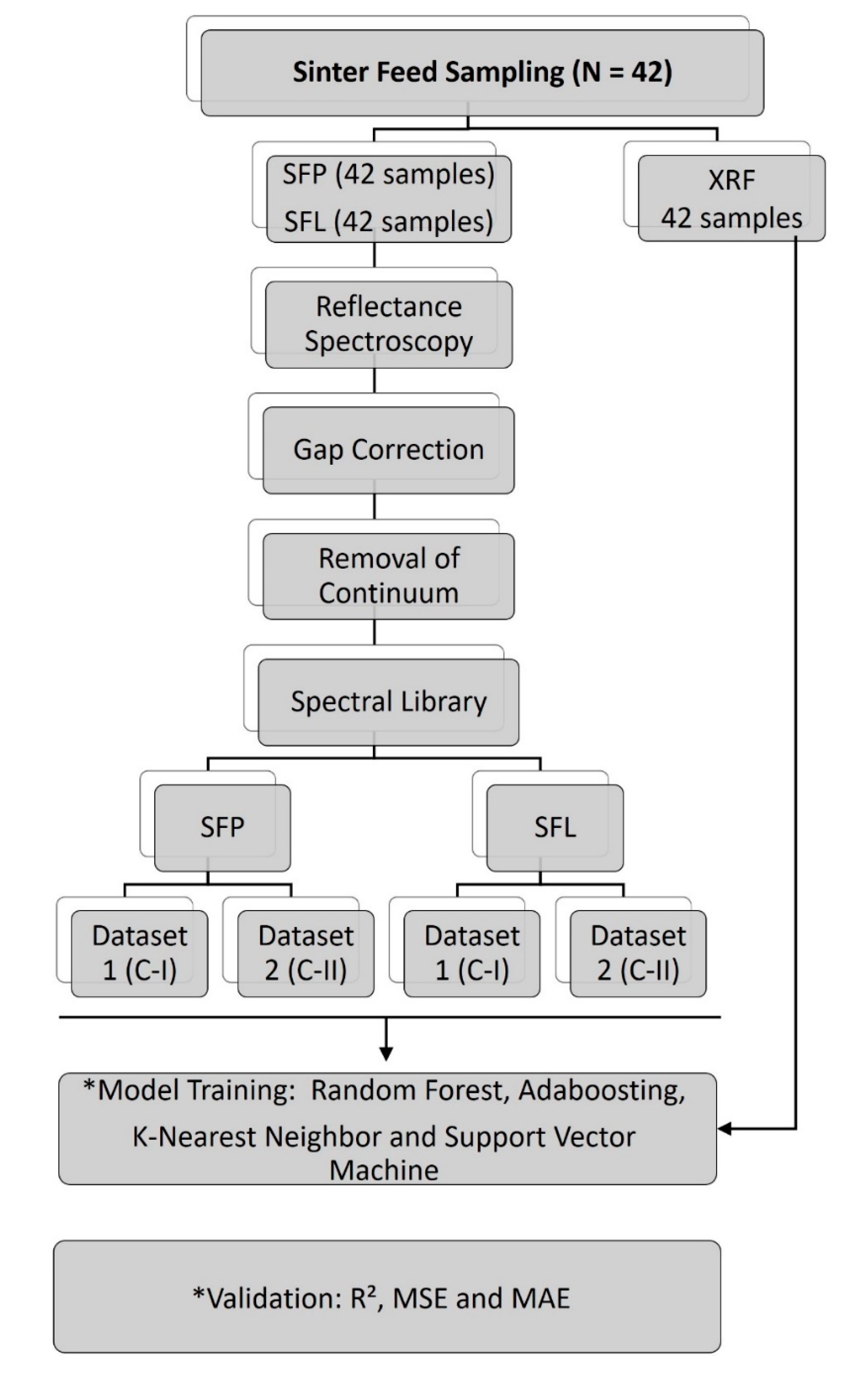
2. Materials and Methods

In this study, two groups of samples were used, which included the Sinter Feed Product (SFP) and Sinter Feed prepared in the laboratory (SFL), as well as their respective chemical analyses performed by XRF. The methodology used follows the flowchart in Figure 2 and is detailed in the following section.
Table 1 shows the XRF analyses of the studied samples. The data were organized according to the nomenclature of the samples and the arrangement of the respective major and minor elements. In turn, in the lower rows of the table, there is the mean and the demonstration of the minimum and maximum values of each element analyzed.

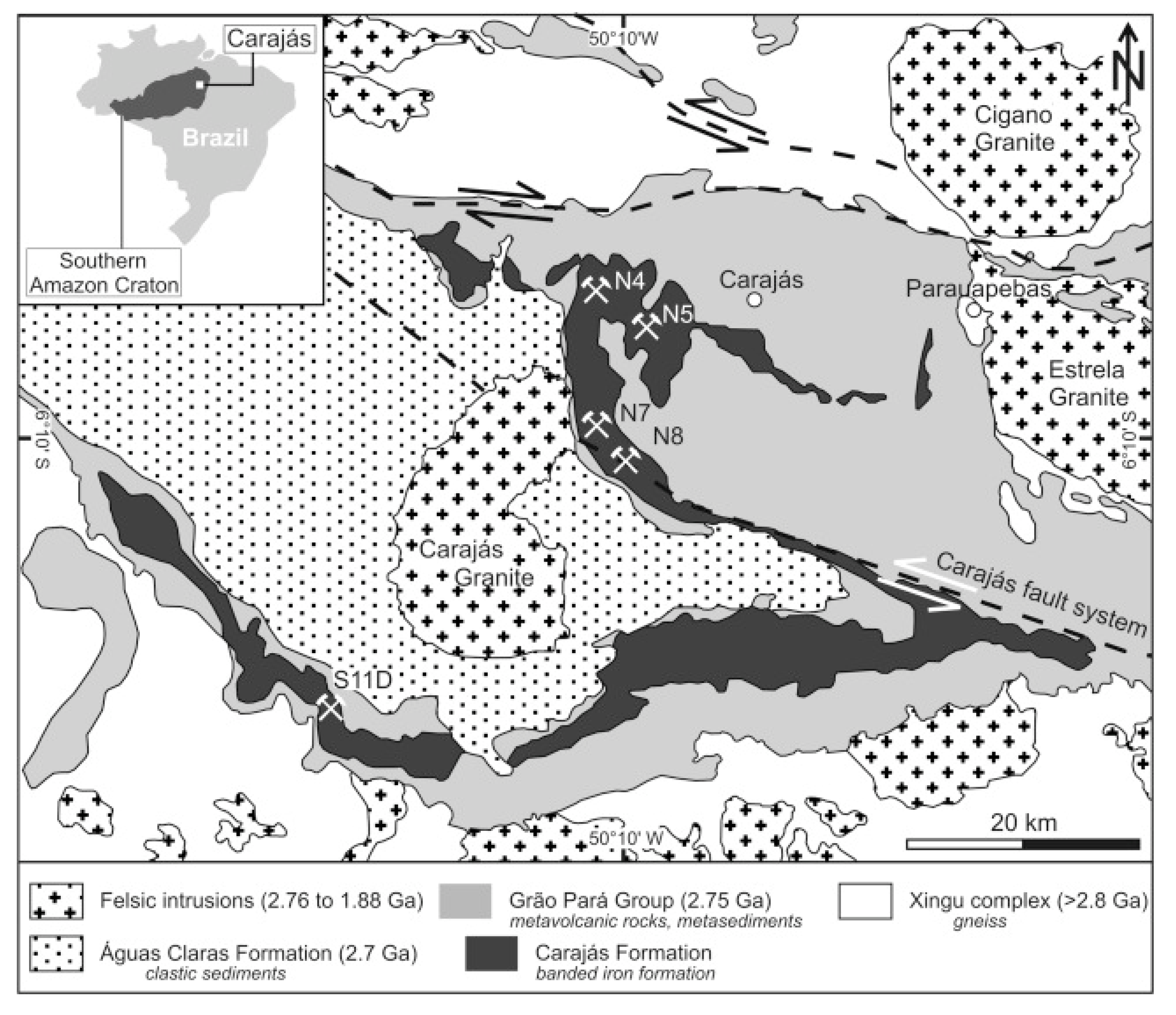
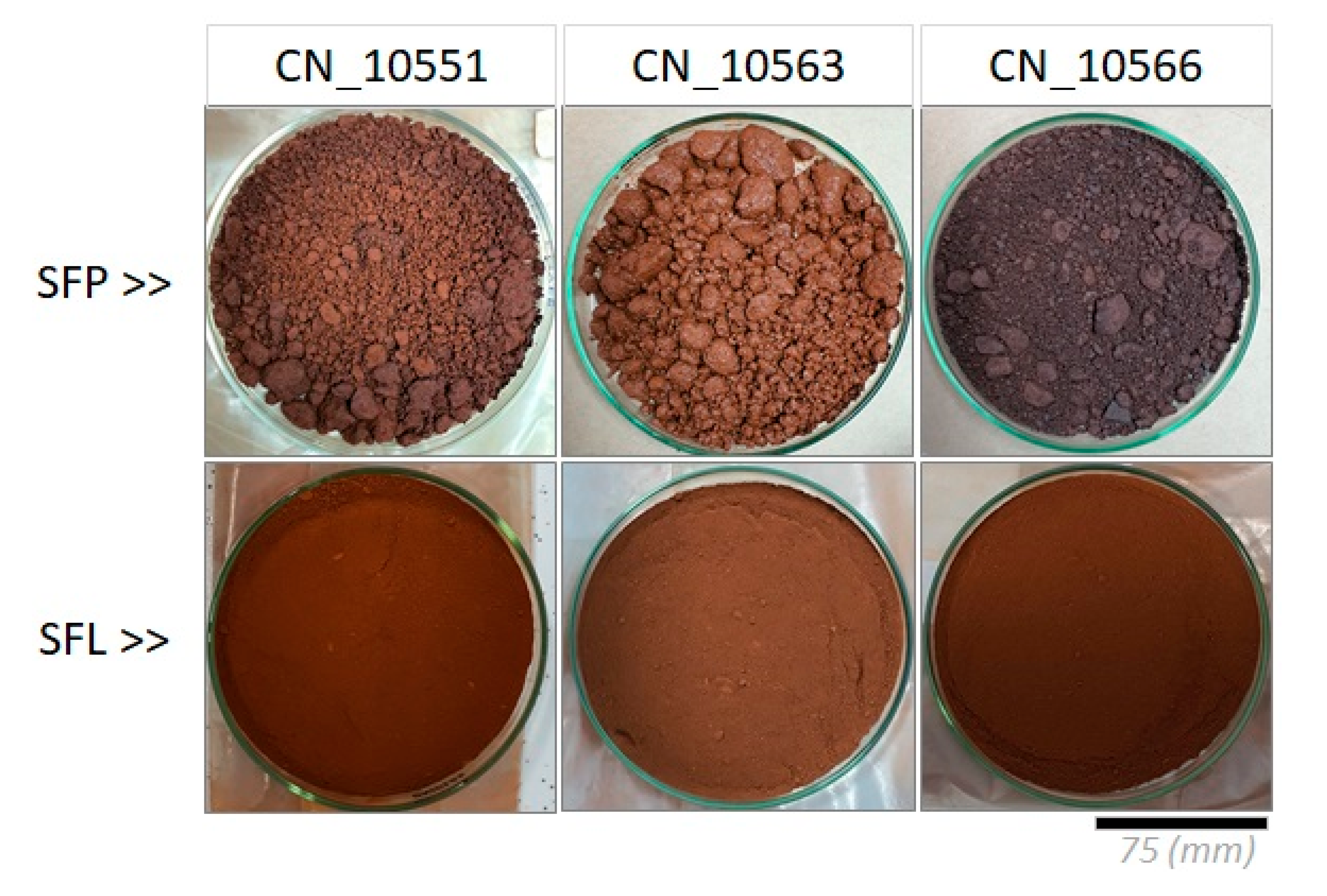
2.1. Sinter Feed Samples

In this study, the database containing Sinter Feed samples and their respective XRF analyses was extracted from [20]. The samples were divided into two groups (Figure 3). The first group comprises 42 samples of SFP, which corresponds to the material of the crushed mining front and has a particle size ranging from 6.3 to 0.150 mm. The second group includes the same 42 samples of SFL that underwent spraying and drying processes, resulting in a more homogeneous particle size.

2.2. Acquisition and Processing of Reflectance Spectra

The instrument used to acquire the reflectance data in the VSWIR interval was the FieldSpec 4 High-Resolution Next Generation high-resolution spectroradiometer coupled with the Turntable reading device, both of which are from the Analytical Spectral Devices manufacturer [21]. FieldSpec 4 Hi-Res NG detects electromagnetic radiation in the spectral range between 350 nm and 2500 nm, with spectral resolutions of 3 nm (@700 nm) and 6 nm (@1400 nm/2100 nm). The sampling intervals are 1.4 nm between 350–1000 nm and 1.1 nm in the range of 1000–2500 nm, with 2151 channels. The reflectance data were generated from measurements of energy reflected by the target in relation to a reference material (Spectralon) in the entire VSWIR range.
The reading of the spectra was performed using RS3 software in conjunction with Turntable and FieldSpec 4 equipment. The samples were placed in Petri dishes with dimensions of 150 mm × 15 mm to obtain readings through the spectroradiometer. Each sample was measured 100 times with 50 scans. Thus, each spectrum used in the spectral characterization corresponds to an average of 5000 readings.
In the preprocessing step of the spectra, gap correction was performed, considering that the FieldSpec 4 Hi-Res NG has three different sensors, and in the sequence, the average of the 100 spectral readings collected was calculated. This procedure allows the reduction in noise and artifacts that may hinder the interpretation of the absorption features.
The corrected spectra were processed using open-source software ViewSpecPro version 6.2.0 [21]. In this step, the continuum was removed, the main purpose of which was to eliminate or reduce the effects unrelated to the properties of interest for the analyzed targets and to highlight the absorption features of the spectra [22,23,24]. The continuum removal technique generates normalized data, in which all information is represented on the same order of magnitude, on a scale of zero to one, and it is compared with the same level of relevance.
Finally, after processing the spectra, wavelength versus reflectance factor plots were prepared to compose the spectral libraries with the SFP and SFL data.

2.3. Datasets

To calibrate and validate the models, two datasets were organized for SFP and two were organized for SFL, with the first considering the broadest spectrum in the range of 400 to 2500 nm (Calibration 1, or C-I) and the second considering the range of 400 to 1310 nm (Calibration 2, or C-II). The C-II data focused on the characteristic features of iron oxides and hydroxides, which are generally observed in the visible and near-infrared (VNIR) region at 670, 860 and 900 nm.

2.3.1. Modeling Procedures

The spectral measurements were acquired in the SFP (n = 42) and SFL (n = 42) samples. For each sample, 100 spectral readings were performed, considering an average of 25 readings, resulting in four spectra per sample and a database of 169 spectra for SFP and 169 for SFL.
The models were trained to estimate the iron contents of the sample sets from the regression relationship found by the machine learning methods, the spectral bands and the iron contents analyzed by XRF. In the composition of the database, 70% of the data were used for training (118 spectra) and 30% were used for model validation (51 spectra). The selection of samples for training and validation of the methods was performed randomly. In the case of training, the C-I and C-II datasets organized for both SFP and SFL were used.
Models that have shown satisfactory results in studies developed by different authors involving reflectance spectroscopy were tested [14,15]. Among these models, four that showed the best performance for the dataset analyzed were selected in this study: the Random Forest (RF); Adaboost (ADB); K-Nearest Neighbor (k-NN); and support vector machine (SVM).
The software used in this step was Orange Canvas, which is open source and has data visualization through streams. The choice of Orange Canvas was based on its characteristic of qualitative analysis, where the graphical interface allows a greater focus on exploratory analysis of the data instead of programming codes. It already has several open-source Python libraries, such as numpy, scipy and scikit-learn, and thus, several machine learning algorithms are available for testing and evaluating models [25].

2.3.2. Random Forest (RF)

An RF comprises a set of decision trees that vote together for a classification. Each tree is constructed by chance and randomly selects a subset of resources from a subset of data points. The tree is trained in these data points (only in the selected characteristics), and the rest “out of the basket” are used to evaluate the tree. RF is known to be effective in preventing overfitting [26]. After reaching a certain number of trees, the overfitting remains constant, and no superior performance is achieved.
This method works efficiently on large volumes of data as it works with the training data and thus the algorithm seeks the best conditions and where to insert each one into the flow [27].
For this study, 30 trees were used, with several attributes considered in each division of five. In the tests, it was observed that values greater than 30 did not bring performance gains in the result and thus would result only in computational overload.

2.3.3. Adaboosting (ADB)

The ADB is a machine learning method that uses multiple classifiers based on a combination of classifiers with lower accuracy, where the result produces a classifier with higher accuracy. Thus, for data training, the method induces the interaction of these various classifier models, and at each interaction, the boosting method generates a hypothesis. Each new hypothesis generated has the objective of correcting the errors resulting from the previously tested hypotheses. The process is repeated until the training stage is completed [28].
A total of 100 tree-type estimators were adopted, with a maximum learning rate of one. The criterion adopted was empirical, and the increase in the number of estimators above that adopted did not result in a significant improvement in performance for the model.

2.3.4. K-Nearest Neighbor (kNN)

The kNN algorithm is a simple model used in both classification and regression problems that predict future values based on past recorded values. In this method, the variable “K” will direct the number of neighbors; thus, the algorithm searches for the desired values closest to that point based on the distances of its “K” closest neighbors [29].
According to [30], the calculation to determine the closest neighbors can be performed using various mathematical methods to calculate the distance between two points, according to the following equations:
Euclidean distance : d ( p , q ) = i = 1 n σ q i 2
Distance from Manhatten : d ( p , q ) = i = 1 n | σ q i |
Mahalanobis distance : d ( p , q ) = i = 1 n σ q i 2 π i 2
Chebyshev distance : d ( p , q ) = max k σ k q ik
In determining the values to be assigned to “K”, if they are very low, they will be affected by noise in the data to influence the final result obtained, which makes it more sensitive to very close regions, which may result in overfitting. However, very high values, with the generation of several neighbors, can generate more robust models [31].
The metric adopted for the method was the Euclidean distance, with uniform weights, which showed the best performance based on empirical tests. The number of neighborhoods used was 10, specified by calculating the approximate square root of the total number of data applied to train the model.

2.3.5. Support Vector Machine (SVM)

The SVM was initially developed with a focus on the solution to binary classification problems. Subsequently, the technique was improved and used for multiclass classification and regression problems [32].
The concept of SVM is the separation of data into classes; for this purpose, the algorithm creates hyperplanes, where each data point belongs to the training base and is plotted as a point in n-dimensional space and with reference to a coordinate. Thus, classification is performed with the objective of finding the hyperplane that will differentiate classes [11].
The parameters adopted for the SVM method were the standard configurations of the estimator present in the Orange Canvas software, with a limit interaction number of 50.

2.4. Validation of Predication Models

Different statistical metrics were used to evaluate the prediction accuracy of the models, including the coefficient of determination (R2), mean absolute error (MAE), and mean square error (MSE) [33,34]. These metrics made it possible to evaluate the accuracy of the machine learning models, comparing the estimated Fe values for each method with the respective levels analyzed by XRF.

3. Results

This section may be divided by subheadings. It should provide a concise and precise description of the experimental results, their interpretation, as well as the experimental conclusions that can be drawn.

3.1. Physical and Spectral Characterization of the Sinter Feed

Figure 4 shows the spectral library used for the calibration and validation datasets of the Fe content estimation models. Figure 4A shows the SFP spectra used for C-I and C-II. Following the same logic, Figure 4B shows the corresponding SFL samples. The graphs show the reflectance values normalized by removal of the continuum on the Y axis and the wavelength on the X axis.
The spectra of the SFP and SFL samples show some similarities; for example, both have absorption features in the VNIR region at approximately 860 and 900 nm. However, when dealing with the sprayed samples, some features were well attenuated, both for VNIR and SWIR. In the case of VNIR, this attenuation was observed at 670 nm, and in SWIR, it was observed at 1400, 1950 and between 2135 and 2500 nm.
The reflectance spectra, as well as photographs of the representative samples of the Sinter Feed, with higher and lower Fe contents, are shown in Figure 5 and Figure 6. In analyzing the spectra, the VNIR region for both SFP and for SFL at 860 nm, has a deep absorption feature for sample CN_10585 and is relatively more discrete for sample CN_10584. Conversely, at 900 nm, marked features are observed for samples CN_10564, CN_10563, CN_10556 and CN_10550 (Figure 5A,B). In the region of 670 nm, for SFP, all samples showed absorption features, which were less pronounced for CN_10585 and CN_10584. For samples prepared in the laboratory, the region’s feature was attenuated (Figure 5B).
Regarding the physical characteristics, the Sinter Feed samples can be divided into two groups: (i) Sinter Feed with particle size ranging from fine to medium, with dark red to black tones. This group is represented by samples CN_10585, CN_10584 and CN_10564, and when subjected to the process of spraying and drying in the laboratory, the black samples tend to result in reddish tones (Figure 5C); (ii) Sinter Feed with coarse particle size, light red tones and cohesive texture. The CN_10563 sample represents this group, and after spraying, it maintained its reddish color (Figure 5C).
In the SWIR region, for SFP at 1380 and 1950 nm, there are features related to H2O and OH (Figure 5A). Conversely, between 2200 and 2500 nm, the features are commonly linked to contaminants, such as Al-OH, Mg-OH, CO3 and OH (Figure 6). These features are observed for nearly all samples in Figure 6, with the exception of CN_10585. For the SFL spectra, these features were masked in all spectra shown in Figure 6.

3.2. Iron Estimation Models

The models tested here, RF, ADB, kNN, and SVM, provided different forecasting precision for the Fe concentrations of the Sinter Feed samples (Table 2). The table with the evaluation statistics of the models was divided into two parts, one with the evaluation of the models calibrated with the SFP samples (A) and another for the SFL samples (B). In both cases, the R2, MSE and MAE statistics are presented for the models calibrated with the spectra of the C-I and C-II libraries.
The models tested with the spectra of the C-I dataset for SFP with the best performances were ADB and SVM (Table 2). In the case of ADB, R2 = 0.801, MSE = 0.479, and MAE = 0.554. For SVM, R2 = 0.865, MSE = 0.325, and MAE = 0.450. On the other hand, the RF and kNN showed lower performances, with R2 < 0.768, MSE and MAE > 0.559. All models trained with the C-II dataset showed lower performance compared to C-I (Table 2), with R2 ranging from 0.627 to 0.758, MSE between 0.584 and 0.898 and MAE between 0.676 and 0.760.
The results of the SFP Fe estimates performed by the tested model dataset C-I can be seen in Figure 7A and with dataset C-II in Figure 7B. In the graphs, the levels of Fe analyzed by XRF are on the X axis, and the levels estimated by the models calibrated in this study are on the Y axis.
Corroborating the results presented in the statistical table, the graphs show that the predictions made with ADB and SVM were more efficient in estimating the Fe content in SFP and C-I (Figure 7A). In this case, the samples are better fitted with the trend lines plotted in the graph. On the other hand, for both RF and kNN, the samples are more scattered and more distant from the line. Furthermore, the graphs of the Fe contents estimated with the C-II dataset also show a large dispersion between samples for the four models tested (Figure 7B).
The models calibrated with the C-I and C-II datasets of the samples of SFL showed very similar performances (Table 2). The best performances are observed in the RF, ADB and SVM models, with R2 ranging from 0.777 to 0.884, MSE between 0.280 and 0.536, and MAE between 0.452 and 0.935. The kNN model had the worst performance, with R2 values between 0.724 and 0.732, MSE values between 0.647 and 0.664, and MAE values between 0.650 and 0.677.
The results of the SFL Fe estimates performed by the models tested with the C-I and C-II datasets were plotted together with the Fe contents analyzed by XRF in the graphs of Figure 8A,B, respectively. In general, the arrangement of the samples in the graphs shows good alignment with the trend line for the RF, ADB and SVM models for both C-I and C-II. In contrast, the samples in the kNN plot are more dispersed for the entire analyzed dataset, thus corroborating the evaluation of the statistical data in Table 2.

4. Discussion

The CMP, together with the Iron Quadrangle (in southeastern Brazil) and Hamersley Province (in western Australia), hosts the largest deposits of high-content Fe in the world [35]. Pioneer studies conducted in the Carajás Province showed that the high-grade ore in the region is commonly associated with paragenesis containing hematite as an essential mineral. However, lower mineralization levels are also associated with intermediate-grade magnetite-carbonate or hematite-carbonate paragenesis, in addition to the formation of banded and goethite formations [36]. In general, high-grade ore occurs in the form of tabular bodies of friable to soft hematite containing smaller lenses of hard hematite [35].
The average percentage of Fe observed in the set of samples studied here is 62%, with the lowest value occurring for sample CN_10584 (41%) and the highest for sample CN_10585 (68%). Regarding the other elements, the means are 2.0% for SiO2, 0.28% for P, 1.74% for Al2O3, 0.021% for Mn, 0.022% for TiO2, 0.040% for MgO, 0.006% for CaO and 0.007% K2O (Table 1).
Samples with lower Fe contents have higher SiO2 contents, for example, as samples CN_10583 (Fe = 58%) and CN_10584 (Fe = 41%), with silica contents of 14 and 39%, respectively, which may represent the reflection of lithological variation and possible associations with the Cangas [20]. In addition to SiO2, it was not possible to observe a very clear relationship between Fe and the other elements analyzed.
Regarding contaminants, especially SiO2, most of the samples are within the expected limit (SiO2 < 0.6%) to maintain the quality of the ore for steel production, using [37] as a reference, except for samples CN_10582, CN_10583 and CN_10584, which have SiO2 contents varying from 9–39%.
Regarding phosphorus (P), the mean content observed in the sample set was approximately 0.2% (Table 1). According to [1], this element is commonly associated with secondary iron oxides, such as limonite, goethite, secondary hematite, and minerals rich in alumina, including clay and gibbsite, and apatite/hydroxyapatite in magnetite ores. Such minerals will influence different regions of the spectrum.
The evaluation of the XRF chemical analyses contributed to interpretation of the spectral curves of the dataset as the physicochemical and mineralogical characteristics of a given material directly influence its reflectance spectra. Such information can be obtained by analyzing the depth and location of the absorption features of each material [38].
In the spectra evaluated here, the most developed absorption features are in the VNIR, which is the region with the best response for the characterization of iron oxides and hydroxides [38]. The features observed at 485 nm (SFL) and 488 nm (SFP) can be explained by the transfer of charges, which are common phenomena in oxides [39].
Pioneering reflectance spectroscopy studies revealed that the position of the absorption feature between 850–1000 nm is a function of the composition of Fe oxides and hydroxides, in which pure hematite is characterized in the range of ~860 nm and pure goethite in ~920 nm [40]. Thus, the comparison of the spectra of the samples illustrated in Figure 5 suggests that samples CN_10585, CN_10584 and CN_10564 are more hematinic, while the others have spectral characteristics of goethite. Nevertheless, in the VNIR region, it is possible to observe that the hematite samples have more subtle absorption features at 670 nm compared to the goethite samples. These features are commonly associated with F3+ [40].
Even if hematite samples are commonly associated with high Fe content [35], it is important to evaluate the presence and influence of contaminants (Figure 6). For example, sample CN_10585 shows a very characteristic spectral curve of hematite, low values of contaminants, such as silica, alumina and P (SiO2 = 1.21; P = 0.01; Al2 O3 = 0.22), and high iron content (Fe = 68%). In turn, between 2200 and 2500 nm, it was not possible to observe significant absorption features for the spectrum of this sample (Figure 6).
In contrast, the CN_10584 sample, which also has a diagnostic spectral curve of hematite (Figure 5), showed an absorption feature close to 2200 nm (Figure 6), which may reflect the presence of the silica observed in Table 1, where SiO2 = 39%. Thus, even if the spectrum suggests the presence of hematite, this sample has the lowest iron content of the studied set (Fe = 41%).
Comparing the spectra of the three goethite samples, it is possible to observe absorption features between 2100 and 2500 nm (Figure 6). These features may be related to the presence of contaminants or even FeOH. The CN_10563 sample exhibits a very subtle feature at approximately 2300 nm, and the XRF result shows a relatively high iron content (Fe = 63%) and no significant contaminant content (SiO2 = 0.62; P = 0.13; Al2O3 = 0.98). Conversely, samples CN_10556 and CN_10550, which have relatively lower iron contents, at approximately 60%, exhibit slightly deeper absorption features in the 2310 nm range, which can be explained by the high phosphorus contents (P = 0.47 a 0.52%) and alumina (Al2 O3 = 2.9 to 3.0%).
The SFP spectra have absorption features at 1380 and 1950 (Figure 5A). These features do not occur for SFL (Figure 5B), and according to Clark (1999), they are commonly associated with the presence of H2O or OH. Regarding the spraying and drying process, within the scope of spectral characterization, the results discussed here showed that there were no significant gains in making the samples homogeneous and without moisture, considering that several absorption features were attenuated for SFL, which made it a factor that hinders qualitative analysis.
Identification of the typical absorption features of hematite and goethite corroborates the information about the Sinter Feed mineralogy extracted from the physical descriptions of the samples. In this case, CN_10585, CN_10584 and CN_10564, which showed features in the 860 nm region (characteristic of hematite), were physically described as friable hematites with fine to medium particle size and dark red to black color when produced, which changed to dark red tones when prepared in the laboratory (Figure 5C). Conversely, the CN_10563 sample selected to represent the group of goethite samples, which showed an absorption feature at approximately 900 nm, has a coarse particle size with a cohesive texture, characteristic of cangas, typical of the Carajás Formation [20]. The sample is also light red when used as a product and darker red when prepared in the laboratory (Figure 5C). Despite its relatively high Fe content, due to its physical characteristics and the presence of impurities, processing the canga is more laborious than processing friable hematite [20].
Comparing the performance of the tested algorithms with the C-I and C-II spectra used to estimate the SF content of Fe, it is not possible to notice very significant differences between them. In both cases, the best estimates were made using the RF, ADB, and SVM models, in which the statistical metrics showed lower MSE and MAE values and the highest R2 values. In contrast, the kNN method showed lower efficiency for estimating Fe contents and was thus less suitable for this purpose.
Regarding the algorithms trained with the SFP spectral library, the best results were achieved using the C-I spectra, with the ADB and SVM being more efficient in estimating the Fe contents. Already restricting the spectrum region, in the case of C-II, none of the algorithms showed satisfactory results, with low R2 values and relatively high MSE and MAE values.
Comparing the best results of the calibrated SFP models with the SFL results, it was found that there is no significant difference between the performance of the models. In the case of the Sinter Feed product (C-I), the ADB and SVM algorithms showed R2 values between 0.801 and 0.865, MSE values between 0.325 and 0.479 and MAE values between 0.450 and 0.554. For SFL (C-I and C-II), the RF, ADB and SVM showed R2 values between 0.777 and 0.884, MSE values between 0.295 and 0.493, and MAE values between 0.451 and 0.935.

5. Conclusions

The main contributions of this study are listed as follows:
-
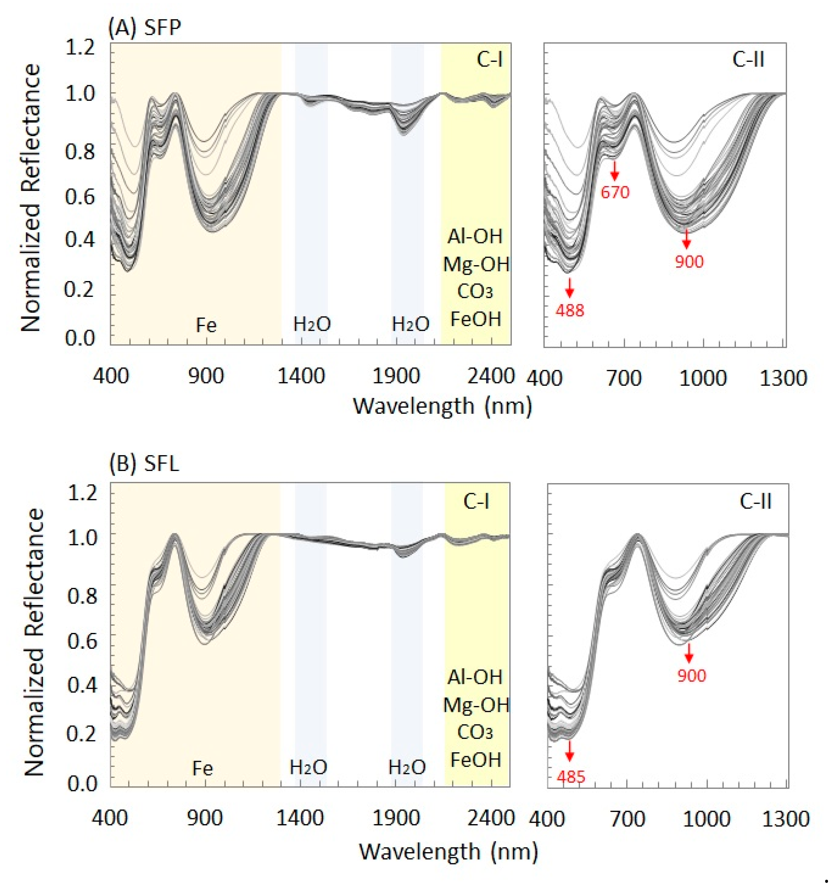
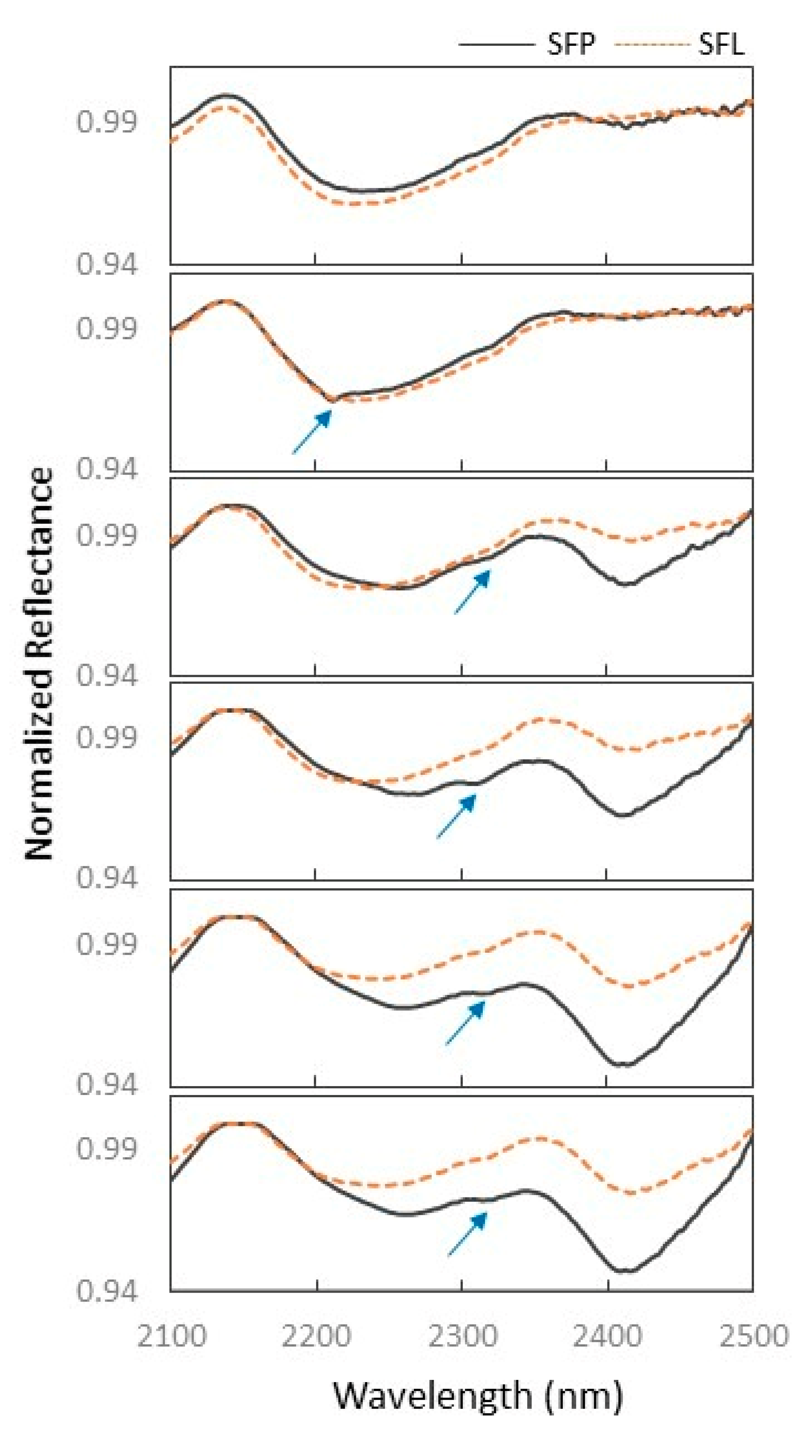
Spectrally, there were no gains with the preparation of the Sinter Feed samples in the laboratory as with the drying and spraying procedures, the particle size of these samples became more homogeneous, thus attenuating the VSWIR absorption features used for qualitative and quantitative analyses of the physicochemical and mineralogical properties of the Sinter Feed.
-
The absorption features located in the VNIR region (~860 nm) enabled the identification of more hematitic (CN_10585, CN_10584 and CN_10564) and goethite samples, starting at 900 nm (CN_10563, CN_10556 and CN_10550). This information corroborated the physical characterization of the Sinter Feed, in which the hematitic samples were described as the most friable material with fine to medium particle sizes and colors between red to black (when product) and dark red (when sprayed). On the other hand, the goethite samples had coarser particle sizes and colors varying in shades of red, both for the Sinter Feed product samples and for the samples prepared in the laboratory.
-
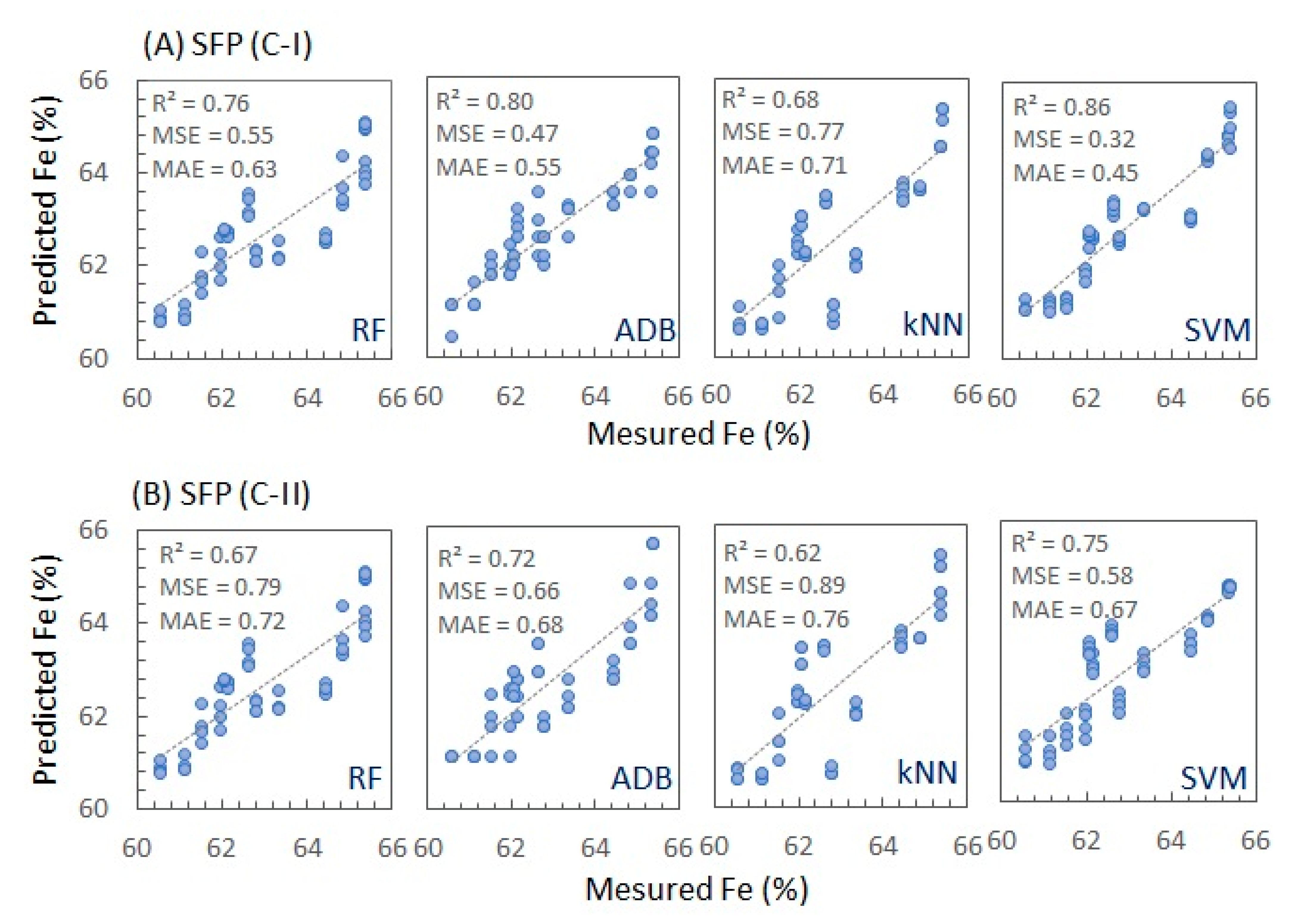
The best Fe estimates for SFP were made with the ADB and SVM models, using only the C-I dataset, which is in the spectral range of 400 to 2500 nm.
-
For SFL, the RF, ADB and SVM models were more efficient for estimating Fe using both the C-I and C-II libraries. Conversely, kNN is the least recommended for this application.
-
The possibility of calibrating models, such as SVM and ADB, using only the Sinter Feed spectra without sample preparation opens space to discuss the operationalization of these methods in the processing plant routine.
-
Finally, we suggest calibration and evaluation of models using reflectance spectroscopy and XRF to estimate contaminants, such as phosphorus, silica, manganese and alumina. We also suggest that other algorithms could be tested to improve the results presented here, such as decision trees and artificial neural networks.

Author Contributions

A.C.P.S.: Conceptualization, methodology, software, data curation, validation, formal analysis, writing—original draft preparation; K.T.Z.C.: Conceptualization, methodology, formal analysis, Writing—review and editing, Supervision, L.W.R.F.: Software, validation, formal analysis, G.P.: Conceptualization, methodology, formal analysis, Writing—review and editing, Supervision, R.E.C.-P.: Conceptualization, methodology, formal analysis, Writing—review and editing, Supervision, project administration. All authors have read and agreed to the published version of the manuscript.

Funding

This research was in part by the Coordenação de Aperfeiçoamento de Pessoal de Nível Superior—Brasil (CAPES)—Finance Code 001, the Conselho Nacional de Desenvolvimento Científico e Tecnológico (CNPQ), the Instituto Tecnológico Vale (ITV) and the Universidade Federal de Ouro Preto (UFOP).

Data Availability Statement

Not applicable.

Acknowledgments

We Thank Vale—Serra Sul Physical Chemical Laboratory for providing the sinter feed iron ore samples, as laboratory tests results. We also would like to acknowledge The ITV for supporting the research, as well as providing all the equipment that made it possible to accomplish the spectral readings.

Conflicts of Interest

The authors declare no conflict of interest. The funders had no role in the design of the study; in the collection, analyses, or interpretation of data; in the writing of the manuscript, or in the decision to publish the results.

References

  1. Yellishetty, M.; Werner, T.T.; Weng, Z. Iron Ore in Australia and the World: Resources, Production, Sustainability, and Future Prospects. In Iron Ore; Woodhead Publishing: Cambridge, UK, 2022; pp. 711–750. [Google Scholar]
  2. Banco de Desenvolvimento de Minas Gerais. Minas Gerais Do Século XXI. Vol.IX. Belo Horizonte: Rona Editora. 2002. Available online: https://silo.tips/download/minas-gerais-do-seculo-xxi-2 (accessed on 23 March 2022).
  3. Grainger, C.J.; Groves, D.I.; Tallarico, F.H.; Fletcher, I.R. Metallogenesis of the Carajás mineral province, southern Amazon craton, Brazil: Varying styles of Archean through Paleoproterozoic to Neoproterozoic base-and precious-metal mineralisation. Ore Geol. Rev. 2008, 33, 451–489. [Google Scholar] [CrossRef]
  4. Juliani, C.; Monteiro, L.V.S.; Fernandes, C.M.D. Potencial Mineral: Cobre. In Recursos Minerais no Brasil: Problemas e Desafios; Melfi, A.J., Misi, A., Campos, D.d.A., Cordani, U.G., Eds.; Academia Brasileira de Ciências: Rio de Janeiro, Brazil, 2006; pp. 134–149. [Google Scholar]
  5. Cabral, A.; Creaser, R.; Nägler, T.; Lehmann, B.; Voegelin, A.; Belyatsky, B.; Pašava, J.; Gomes, A.S.; Galbiatti, H.; Böttcher, M.E.; et al. Trace-element and multi-isotope geochemistry of Late-Archean black shales in the Carajás iron-ore district, Brazil. Chem. Geol. 2013, 362, 91–104. [Google Scholar] [CrossRef]
  6. Xiao, D.; Le, B.T.; Ha, T.T.L. Iron ore identification method using reflectance spectrometer and a deep neural network framework. Spectrochim. Acta Part A Mol. Biomol. Spectrosc. 2021, 248, 119168. [Google Scholar] [CrossRef] [PubMed]
  7. Lobo, A.; Garcia, E.; Barroso, G.; Martí, D.; Fernandez-Turiel, J.-L.; Ibáñez-Insa, J. Machine Learning for Mineral Identification and Ore Estimation from Hyperspectral Imagery in Tin–Tungsten Deposits: Simulation under Indoor Conditions. Remote Sens. 2021, 13, 3258. [Google Scholar] [CrossRef]
  8. Tuşa, L.; Kern, M.; Khodadadzadeh, M.; Blannin, R.; Gloaguen, R.; Gutzmer, J. Evaluating the performance of hyperspectral short-wave infrared sensors for the pre-sorting of complex ores using machine learning methods. Miner. Eng. 2020, 146, 106150. [Google Scholar] [CrossRef]
  9. Barra, I.; Haefele, S.M.; Sakrabani, R.; Kebede, F. Soil spectroscopy with the use of chemometrics, machine learning and pre-processing techniques in soil diagnosis: Recent advances—A review. TrAC Trends Anal. Chem. 2021, 135, 116166. [Google Scholar] [CrossRef]
  10. Brown, D.J.; Shepherd, K.D.; Walsh, M.G.; Mays, M.D.; Reinsch, T.G. Global soil characterization with VNIR diffuse reflectance spectroscopy. Geoderma 2006, 132, 273–290. [Google Scholar] [CrossRef]
  11. Chen, S.H.; Jakeman, A.J.; Norton, J.P. Artificial Intelligence techniques: An introduction to their use for modelling environmental systems. Math. Comput. Simul. 2008, 78, 379–400. [Google Scholar] [CrossRef]
  12. Richter, N.; Jarmer, T.; Chabrillat, S.; Oyonarte, C.; Hostert, P.; Kaufmann, H. Free Iron Oxide Determination in Mediterranean Soils using Diffuse Reflectance Spectroscopy. Soil Sci. Soc. Am. J. 2009, 73, 72–81. [Google Scholar] [CrossRef]
  13. Rossel, R.V.; Behrens, T. Using data mining to model and interpret soil diffuse reflectance spectra. Geoderma 2010, 158, 46–54. [Google Scholar] [CrossRef]
  14. Khosravi, V.; Ardejani, F.D.; Yousefi, S.; Aryafar, A. Monitoring soil lead and zinc contents via combination of spectroscopy with extreme learning machine and other data mining methods. Geoderma 2018, 318, 29–41. [Google Scholar] [CrossRef]
  15. Hu, P.; Liu, X.; Cai, Y.; Cai, Z. Band Selection of Hyperspectral Images Using Multiobjective Optimization-Based Sparse Self-Representation. IEEE Geosci. Remote Sens. Lett. 2018, 16, 452–456. [Google Scholar] [CrossRef]
  16. Pabón, R.E.C.; Filho, C.R.D.S.; de Oliveira, W.J. Reflectance and imaging spectroscopy applied to detection of petroleum hydrocarbon pollution in bare soils. Sci. Total Environ. 2019, 649, 1224–1236. [Google Scholar] [CrossRef] [PubMed]
  17. Cardoso-Fernandes, J.; Silva, J.; Lima, A.; Teodoro, A.C.; Perrotta, M.; Cauzid, J.; Roda-Robles, E.; Ribeiro, M.D.A. Reflectance spectroscopy to validate remote sensing data/algorithms for satellite-based lithium (Li) exploration (Central East Portugal). In Earth Resources and Environmental Remote Sensing/GIS Applications XI; International Society for Optics and Photonics: Bellingham, WA, USA, 2020; Volume 11534. [Google Scholar]
  18. Jia, X.; O’Connor, D.; Shi, Z.; Hou, D. VIRS based detection in combination with machine learning for mapping soil pollution. Environ. Pollut. 2021, 268, 115845. [Google Scholar] [CrossRef]
  19. Parent, E.J.; Parent, S.É.; Parent, L.E. Machine learning prediction of particle-size distribution from infrared spectra, methodologies and soil features. bioRxiv 2020. [Google Scholar] [CrossRef]
  20. Silva, A.C.P. Monitoramento da Qualidade de Sinter Feed Através de Dados Espectrais Associados a Aprendizado de Máquina–estudo de Caso: Mina De Carajás Serra Sul (S11D). Master’s Thesis, UFOP, ITV, Ouro Preto, Minas Gerais, Brazil, 2021. Available online: https://www.itv.org/wp-content/uploads/2022/01 (accessed on 20 January 2022).
  21. ASD FieldSpec® 4 Hi-Res: Espectrorradiômetro de Alta Resolução, Malvern Panalytical. Available online: https://www.malvernpanalytical.com/br/products/product-range/asd-range/fieldspec-range (accessed on 17 January 2022).
  22. Clark, R.N.; Roush, T.L. Reflectance spectroscopy: Quantitative analysis techniques for remote sensing applications. J. Geophys. Res. Earth Surf. 1984, 89, 6329–6340. [Google Scholar] [CrossRef]
  23. Kokaly, R.F. Investigating a Physical Basis for Spectroscopic Estimates of Leaf Nitrogen Concentration. Remote Sens. Environ. 2001, 75, 153–161. [Google Scholar] [CrossRef]
  24. Ozaki, Y.; McClure, W.F.; Christy, A.A. (Eds.) Near-Infrared Spectroscopy in Food Science and Technolog; John Wiley & Sons: Hoboken, NJ, USA, 2006. [Google Scholar]
  25. Orange Data Mining. Available online: https://github.com/biolab/orange3 (accessed on 15 January 2022).
  26. Cutler, A.; Cutler, D.R.; Stevens, J.R. Random Forests. In Ensemble Machine Learning; Springer: Boston, MA, USA, 2012; pp. 157–175. [Google Scholar]
  27. Biau, G.; Scornet, E. A random forest guided tour. Test 2016, 25, 197–227. [Google Scholar] [CrossRef] [Green Version]
  28. Borges, F.A.; Rabelo, R.A.; Araujo, M.A.; Fernandes, R.A. Metodologia baseada no algoritmo adaboost combinado com rede reural Para localização do distúrbio de afundamento de tensão. In Congresso Brasileiro de Automática-CBA; Cidade Universitária Zeferino Vaz: Campinas, Brazil, 2019; Volume 1. [Google Scholar]
  29. Alpaydin, E. Introduction to Machine Learning; MIT Press: Cambridge, MA, USA, 2020. [Google Scholar]
  30. Linden, R. Técnicas de Agrupamento. Rev. Sist. Inf. FSMA 2009, 4, 18–36. [Google Scholar]
  31. Lantz, B. Machine Learning with R: Expert Techniques for Predictive Modeling; Packt Publishing Ltd.: Birmingham, UK, 2019. [Google Scholar]
  32. Filgueiras, P.R. Regressão Por Vetores de Suporte Aplicado na Determinação de Propriedades Físico-Químicas de Petróleo e Biocombustíveis. Ph.D. Thesis, Instituto de Química, Universidade Estadual de Campinas, Campinas, Brazil, 2014. [Google Scholar]
  33. Gupta, H.V.; Kling, H.; Yilmaz, K.K.; Martinez, G.F. Decomposition of the mean squared error and NSE performance criteria: Implications for improving hydrological modelling. J. Hydrol. 2009, 377, 80–91. [Google Scholar] [CrossRef] [Green Version]
  34. De Myttenaere, A.; Golden, B.; Le Grand, B.; Rossi, F. Mean absolute percentage error for regression models. Neurocomputing 2016, 192, 38–48. [Google Scholar] [CrossRef] [Green Version]
  35. Clout, J.; Manuel, J. Mineralogical, chemical, and physical characteristics of iron ore. In Iron Ore; Woodhead Publishing: Cambridge, UK, 2015; pp. 45–84. [Google Scholar] [CrossRef]
  36. Dalstra, H.; Guedes, S. Giant hydrothermal hematite deposits with Mg-Fe metasomatism: A comparison of the carajas, hamersley, and other iron ores. Econ. Geol. 2004, 99, 1793–1800. [Google Scholar] [CrossRef]
  37. Upadhyay, R.; Venkatesh, A.S. Current strategies and future challenges on exploration, beneficiation and value addition of iron ore resources with special emphasis on iron ores from Eastern India. Appl. Earth Sci. 2006, 115, 187–195. [Google Scholar] [CrossRef]
  38. Van Der Meer, F. Analysis of spectral absorption features in hyperspectral imagery. Int. J. Appl. Earth Obs. Geoinf. 2004, 5, 55–68. [Google Scholar] [CrossRef]
  39. Pontual, S.; Merry, N.; Gamson, P. Spectral Interpretation-Field Manual. GMEX. Spectral Analysis Guides for Mineral Exploration; AusSpec International Pty. Ltd.: Warrnambool, VIC, Australia, 2008; p. 189. [Google Scholar]
  40. Townsend, T.E. Discrimination of iron alteration minerals in visible and near-infrared reflectance data. J. Geophys. Res. Earth Surf. 1987, 92, 1441–1454. [Google Scholar] [CrossRef]
Figure 1. Geological map showing the Carajás Mineral Province in the context of the Amazonian Craton [5].
Ai 03 00032 g001
Figure 2. Flowchart showing the methodology used: * SFP—Sinter Feed Product; SFL—Sinter Feed Prepared in Laboratory; XRF-X-ray Fluorescence; R2—coefficient of determination; MSE—mean square error; MAE—mean absolute error.
Ai 03 00032 g002
Figure 3. Photographs of the Sinter Feed product samples and their corresponding samples prepared in the laboratory.
Ai 03 00032 g003
Figure 4. Reflectance spectra normalized by removal of the continuum from the samples used in model training: (A) Spectra obtained in the SFP samples, showing the database used for C-I and C-II; (B) Mean of the SFL spectra used for C-I and C-II. The absorption bands relevant to the study are highlighted in the spectra. SFP—Sinter Feed Product; SFL—Sinter Feed prepared in the laboratory; C-I—Calibration 1; C-II—Calibration 2.
Ai 03 00032 g004
Figure 5. (A,B) Reflectance spectra normalized by removing the continuum of sinter feed product (SFP) samples and their equivalent prepared in the laboratory (SFL). The diagnostic features of hematite (Ht) samples, which can be observed at 860 nm (CN_10585, CN_10584, and CN_10564), and goethiteitic (Gt) samples, which occur close to 900 nm, stand out in both the SFP and SFL spectra (samples CN_10563, CN_10556 and CN_10550). The absorption features that occur at 670 nm, which indicates F3+, and at 1380 and 1950 nm, which indicate the presence of H2O, occur only in the SFP spectra and are attenuated in the SFL spectra. (C) Comparison of the SFP and SFL samples showing the physical characteristics of representative samples of higher and lower Fe contents.
Ai 03 00032 g005
Figure 6. Reflectance spectra normalized by removing the continuum of sinter feed product (SFP) samples and their equivalent prepared in the laboratory (SFL). The figure shows in detail the absorption features in the SWIR region that occur mainly for SFP.
Ai 03 00032 g006
Figure 7. (A) Results of the models for estimating Fe tested with the SFP samples with the C-I spectra, showing better ADB and SVM performances. (B) Results of the models for estimating Fe tested with the SFP samples with the C-II spectra, showing that the models were not efficient in estimating the Fe content when reducing the spectrum to 400–1310 nm.
Ai 03 00032 g007
Figure 8. (A,B) Results of the models for the estimation of Fe tested with the Sinter Feed samples prepared in the laboratory with the C-I and C-II spectra, respectively. The graphs show good alignment of the samples for RF, ADB and SVM. For kNN, the samples are more dispersed.
Ai 03 00032 g008
Table 1. X-ray fluorescence (XRF) data of the 42 samples used for model validation training. Column 1 shows the nomenclature of the samples, the first row is the analyzed elements, and the lower portion of the table shows the basic statistical analyses.
SampleFeSiO2PAl2O3MnTiO2CaOMgOK2O
CN_1055161.120.390.432.820.0180.4020.0060.0300.006
CN_1055261.760.400.462.490.0180.4070.0060.0270.007
CN_1055461.990.430.412.440.0190.2530.0060.0270.006
CN_1055660.450.350.522.900.0180.4820.0060.0260.005
CN_1055860.460.320.542.930.0180.4970.0060.0250.005
CN_1056061.130.340.462.420.0180.4040.0060.0260.007
CN_1056162.560.450.321.940.0200.1900.0060.0280.007
CN_1056363.260.480.261.690.0200.2450.0060.0340.008
CN_1056464.000.670.211.470.0220.1760.0060.0350.010
CN_1056663.560.590.251.580.0200.1670.0060.0270.011
CN_1056861.930.410.412.150.0180.4240.0060.0250.007
CN_1056962.450.400.321.770.0180.1970.0060.0250.007
CN_1057363.940.890.211.520.0110.2000.0060.0250.004
CN_1057463.890.630.221.440.0150.1920.0060.0300.004
CN_1057661.610.580.371.880.0080.2390.0060.0250.004
CN_1057762.770.930.271.450.0120.2150.0060.0250.004
CN_1057863.180.460.261.430.0080.2190.0060.0250.004
CN_1057962.180.580.232.680.0100.2790.0080.0250.004
CN_1058063.540.660.211.450.0150.2040.0060.0250.004
CN_1058162.430.630.182.450.0100.2310.0060.0250.004
CN_1058261.989.650.010.410.1120.0420.0060.1000.004
CN_1058358.2114.910.010.600.1340.0480.0060.1050.004
CN_1058441.4139.450.010.370.0230.0670.0060.0960.004
CN_1058568.241.210.010.220.0380.0400.0060.1240.004
CN_1075962.920.580.352.270.0100.1900.0070.0500.009
CN_1076064.370.630.361.330.0150.0840.0070.0570.012
CN_1076265.660.720.140.970.0130.0820.0080.0620.016
CN_1076464.800.560.171.180.0110.1310.0080.0460.009
CN_1076566.110.710.060.600.0160.0680.0080.0640.010
CN_1055361.970.390.382.250.0180.2570.0060.0270.007
CN_1055762.150.570.362.290.0180.1600.0060.0310.007
CN_1055961.120.360.462.440.0180.4100.0060.0250.006
CN_1056263.340.470.291.610.0190.1900.0060.0280.007
CN_1056564.440.490.231.290.0200.1390.0060.0340.007
CN_1056762.060.510.352.410.0190.4180.0060.0270.008
CN_1057562.620.820.221.970.0150.2240.0060.0250.004
CN_1075762.780.560.451.900.0100.1260.0060.0430.009
CN_1076164.850.600.261.270.0090.0990.0070.0450.013
CN_1076365.350.620.130.980.0100.0940.0070.0460.010
CN_1076665.380.610.131.110.0140.1310.0070.0560.008
CN_1055060.550.380.473.030.0170.4360.0060.0280.004
CN_1055563.260.480.261.690.0200.2450.0060.0340.008
Min41.410.320.010.220.0080.0400.0060.0250.004
Max68.2439.450.543.030.1340.4970.0080.1240.016
Average62.422.040.281.740.0210.2220.0060.0400.007
Table 2. Results of the model statistics for the estimation of Fe contents using the reference spectra (C-I and C-II) and the XRF analyses.
(A) SFP
* C-I: 400 to 2500 nn
ModelR2MSEMAE
RF0.7680.5590.638
ADB0.8010.4790.554
kNN0.6800.7710.717
SVM0.8650.3250.450
* C-II: 400 to 1310 nm
RF0.6700.7950.728
ADB0.7250.6620.685
kNN0.6270.8980.760
SVM0.7580.5840.676
(B) SFL
* C-I: 400 to 2500 nm
ModelR2MSEMAE
RF0.7770.5360.567
ADB0.8370.3920.507
kNN0.7240.6640.677
SVM0.8780.2950.451
* C-II: 400 to 1310 nm
RF0.8840.2800.452
ADB0.8720.3080.935
kNN0.7320.6470.650
SVM0.7950.4930.569
Publisher’s Note: MDPI stays neutral with regard to jurisdictional claims in published maps and institutional affiliations.

